Forward Premium Puzzle

Forward Premium Puzzle

By

Danai Tanamee

Submitted to the graduate degree program in Economics and the Graduate Faculty of the

University of Kansas in partial fulfillment of the requirements for the degree of Doctor of

Philosophy.

________________________________

Chairperson Shigeru Iwata

________________________________

Shu Wu

________________________________

Ted Juhl

________________________________

Paul Comolli

________________________________

Bozenna Pasik-Duncan

Date Defended: April 18, 2014

ii

The Dissertation Committee for Danai Tanamee

Certifies that this is the approved version of the following dissertation:

Forward Premium Puzzle

________________________________

Chairperson Shigeru Iwata

Date approved: April 18, 2014

iii

Abstract

Financial liberalizations in recent decades have prepared the way for the rapidly

increasing number of studies related to the investigations of foreign exchange market

efficiency in developing economies via testing for the uncovered interest parity (UIP)

condition. Chapter 1 provides a survey on this recent literature. Specifically, it attempts to

answer the following question: are the economies of developing countries different from

those of developed countries in the context of the UIP condition?

Examining cross-country data, Bansal and Dahlquist (2000) found that the puzzling

correlation between the exchange rate changes and the interest rate differentials of two

countries appears less puzzling among developing countries than among developed countries.

Several economists come up with new types of theoretical models that can explain the above

new findings [e.g. Alvarez and Atkeson (2005), Baccheta and Wincoop (2005, 2009)].

According to these models, when inflation is low, the exchange rate adjustment tends to be

slow because adjustment is costly. This is why we observe the UIP puzzle in many developed

countries where inflation rates are low. In Chapter 2, we cast doubt on these claims of the

models by empirically examining the cross-country data. In essence, we argue that these

models appear to solve the “nominal puzzle” but cannot solve the “real puzzle” of the UIP

relation. After taking account of the relative PPP effect, we observe the same degree of the

real UIP puzzle in both groups of countries.

The increasing international equity flows relative to bank loans or bonds constitutes a

motivation to investigate a relationship of equity returns and exchange rate change. Under no-

arbitrage condition, the expected returns on home equity market should equal those on the

foreign equity market. This relation is known as the Uncovered Equity Party (UEP). In

iv

Chapter 3, we propose an alternative method, called the UEP Ratio and UIP Ratio, to test the

UEP relation and UIP relation, respectively. Examining time-series data for ten countries

with developed financial markets, we find that UIP is less puzzling than we thought.

Furthermore, unlike the literature, we find that UIP holds better than UEP. In addition, the

UEP regression is a biased predictor of the deviation in UEP.

v

Acknowledgements

My deepest gratitude goes to Professor Shigeru Iwata for many years of great advice,

instruction, and guidance throughout my time in the PhD program. He encouraged me to

develop the independent thinking and research skills necessary to be a successful scholar. I

also would like to express appreciation for my current and previous dissertation committee

members, Professor Shu Wu, Professor Ted Juhl, Professor Paul Comolli, Professor Bozenna

Pasik-Duncan, and Professor Alexandre Skiba, for their insightful comments and

encouragement. In addition, I would like to extend special thanks to all attendants of the

Empirical Coffee Workshop in the Department of Economics for helpful suggestions and

comments. I am also grateful for support from my friends at the University of Kansas. I

appreciate all of their help and friendship over the years. Finally, this dissertation would not

be possible without my family. I am indebted to my parents for a lifetime of patience,

understanding, encouragement, and love. I would also like to thank my parents for their

continuous and wholehearted support throughout this process even though my mom has

battled cancer for the last eight years. Her courage inspires me profoundly.

vi

Contents

Abstract ................................................................................................................................... iii

Acknowledgements .................................................................................................................. v

List of Figures ......................................................................................................................... vii

List of Tables ........................................................................................................................ viii

Chapter 1 .................................................................................................................................. 1

What Have We Learned about the Uncovered Interest? ..................................................... 1

1.1 Introduction .................................................................................................................... 1

1.2 UIP and Developing Countries ...................................................................................... 2

Chapter 2 .................................................................................................................................. 6

Real and Nominal Puzzles of the Uncovered Interest Parity ............................................... 6

2.1 Introduction .................................................................................................................... 6

2.2 Nominal and Real Puzzles ............................................................................................. 8

2.3 Empirical Results ......................................................................................................... 13

2.3.1 Data ..................................................................................................................... 13

2.3.2 Empirical Results ................................................................................................ 14

2.3.3 Robustness Check ............................................................................................... 24

2.4 Conclusion ................................................................................................................... 24

Chapter 3 ................................................................................................................................ 26

Uncovered Equity Parity: Is It Another Puzzle? ................................................................ 26

3.1 Introduction .................................................................................................................. 26

3.2 Model and Estimation .................................................................................................. 29

3.2.1 The Uncovered Equity Parity (UEP) condition .................................................. 29

3.2.2 Estimation ........................................................................................................... 31

3.2.3 The Data Generating Processes .......................................................................... 32

3.3 Results .......................................................................................................................... 38

3.3.1 Data ..................................................................................................................... 38

3.3.2 UEP vs. UIP ........................................................................................................ 38

3.4 Conclusion ................................................................................................................... 45

Chapter 4 ................................................................................................................................ 46

Summary ................................................................................................................................. 46

References ............................................................................................................................... 49

Appendix ................................................................................................................................. 52

vii

List of Figures

Figure 2.1: Exchange Rate Changes and Interest Rate Differentials ....................................... 16

Figure 2.2: The Nominal UIP Regression Coefficients and Average Inflation Rate ............... 18

Figure 2.3: The Nominal vs. Real UIP Regression Coefficients and Average Inflation Rate . 22

Figure 2.4: Exchange Rate Changes, Interest Rate Differentials and Expected Inflation

Differentials .......................................................................................................... 23

Figure A3.1: Distribution of the UIP Ratio (left) and UEP Ratio (right) ................................ 56

Figure A3.2: Empirical Distribution of the UIP Ratio implied by the regressions (left) and

exponential of the Jensen’s Inequality Term (right) .......................................... 60

Figure A3.3: Empirical Distributions of the UEP Ratio implied by the regression, exponential

of the covariance term, and exponential of the Jensen’s Inequality terms ......... 64

viii

List of Tables

Table 2.1: Volatilities Statistics ............................................................................................... 15

Table 2.2: Nominal UIP Regressions....................................................................................... 17

Table 2.3: Relative PPP Regressions ....................................................................................... 20

Table 2.4: Real UIP Regressions ............................................................................................. 21

Table 3.1: UIP Ratio and UEP Ratio ....................................................................................... 39

Table 3.2: UIP Ratio Implied by the Regression ..................................................................... 41

Table 3.3: UEP Ratio Implied by the Regression .................................................................... 43

Table A 2.1: Country Information ........................................................................................... 52

Table A 2.2: Nominal UIP Regressions (1997Q3-2009Q1) .................................................... 53

Table A 2.3: Relative PPP Regressions (1997Q3-2009Q1) .................................................... 53

Table A 2.4: Real UIP Regressions (1997Q3-2009Q1)........................................................... 54

Table A 2.5: Nominal UIP Regressions-Extreme Inflation Cutoffs ........................................ 54

Table A 2.6: Relative PPP Regressions-Extreme Inflation Cutoffs ........................................ 55

Table A 2.7: Real UIP Regressions-Extreme Inflation Cutoffs ............................................... 55

1

Chapter 1

What Have We Learned about the Uncovered Interest?

1.1 Introduction

The uncovered interest parity (UIP) condition is a no-arbitrage condition between

investing in an asset denominated in domestic currency and an asset denominated in foreign

currency such that the expected return from a foreign asset is equal to the return from a

domestic asset as follows:

(1.1)

is the home currency price of the foreign currency. and denote asset interest rates

denominated in domestic and foreign currency, respectively.

Log approximation of equation (1.1) yields

, (1.2)

where , .

In other worlds, according to UIP, a speculator is indifferent between interest bearing

identical assets denominated in different currency. UIP predicts that a high interest currency

tends to depreciate against a low interest rate currency. The conventional way to test for the

existence of UIP is to regress the exchange rate change on interest rate differential relative to

a reference currency as follows:

2

(1.3)

where is an error term, and testing the joint hypothesis of and

Assuming the covered interest parity (CIP) condition1, the UIP condition can also be

estimated by regressing the exchange rate change on the forward premium as follows:

, (1.4)

where is the forward rate.

Alternatively, UIP can be described in terms of excess returns from a carry trade.

Consider the carry trade strategy in which investors borrow from a low interest rate currency

and lend it in high interest rate currency; the excess return of this strategy can be defined by

(1.5)

If UIP holds, payoff from a positive interest rate differential will be offset by the

depreciation of the high interest rate currency such that excess returns should be zero. That is,

(1.6)

1.2 UIP and Developing Countries

The wide-ranging survey performed by Engel (1996) not only rejects UIP hypothesis but

also states that its prediction is of the opposite direction. That is, a high interest rate currency

1 The log approximation of CIP condition:

. Burnside et al. (2006) use the interbank interest rates

for ten countries to test the implication of CIP, finding that the relation does hold.

3

tends to appreciate against a low interest rate currency. This is known as the UIP puzzle or

forward premium puzzle.

Economists have not yet come to agreement on what the clear explanations are for the

UIP puzzle. As an example, researchers such as Lustig and Verdelhan (2007) assert that

aggregate consumption growth in the United States is central to understanding the UIP

condition. Specifically, their work shows that high interest rate currencies usually decrease in

value when US consumption growth is low, and US investors expect to be compensated for

this risk. Conversely, Burnside (2007) disagrees with Lustig’s and Verdelhan’s study and

uses the data from the same study, with a different specification of econometric model, to

show that a model based solely on US consumption growth is not sufficient to explain the

currency risk premium.

In addition, Burnside et al. (2008) studied an unbalanced panel of 20 major currencies

with monthly data spans from 1976 to 2007 using U.S. dollar as a funding currency. For most

of these currencies, the estimated slope coefficient is significantly negative, suggesting

excess return from borrowing in low interest rate currencies and lending in high interest rate

ones. Their study shows that excess return is significantly different from zero, but not

statistically correlated with all single and groups of risk factors. Finally, they assert that

sufficient evidence has not been found to support the idea that a “peso problem”, or other rare

disaster, can be used to explain the UIP puzzle.

Attempting to explain the UIP puzzle, Brunnermeir, Nagel, and Pedersen (2008) released

a study consisting of a panel of nine major currencies from 1986 to 2006 that indicates that

currencies with high interest rates have high negatively skewed excess returns which can be

4

interpreted as “crash risk.” This risk could limit arbitrage in currency speculation causing

deviations from UIP.

Most studies focus on the existence of UIP in major currencies in developed countries.

However, there are a number of recent empirical studies that analyze UIP in both developed

economies and emerging markets. Bansal and Dahlquist (2000) show a difference between

developed and emerging economies by using a panel of weekly data spanning from 1976 to

1998 to test an implication of UIP for twenty-eight advanced and emerging economies. Their

results indicate that the UIP puzzle only exists in developed economies when the U.S. interest

rate is higher than the interest rate of other developed countries. However, the puzzle does

not seem to exist, and the estimate of the slope coefficient of equation (1.6) increases toward

unity in emerging economies.

Conversely, Flood and Rose (2002) perform a study composed of thirteen developed

economies and ten emerging markets using an unbalanced panel of daily data starting in the

early 1990s and thus omitted the pre-1990 period in Bansal and Dahlquist (2000). This is

notable since emerging markets around the world had only started reforming their financial

accounts towards the end of the 1980s and the start of the 1990s. Because the study focused

solely on post-1990 data, it excluded the effects of the aggregate shocks seen in the late

1970s and 1980s on the developed economies from the analysis of the UIP condition. Flood

and Rose (2002) show that the deviation from UIP is less in their data sets than it is in older-

period data. The slope coefficient estimates of UIP regression are positive, but the results

indicate no significant differences between developed and emerging economies.

Frankel and Poonawala (2006) used data from December 1996 to April 2004 to analyze

the forward premium puzzle in twenty-one developed countries and fourteen emerging

5

markets. Their results from an individual country and pooled analysis indicate that the UIP

puzzle is present in developed countries. However, in emerging economies, the slope

coefficient estimates are slightly positive on average. Frankel and Poonawala (2006) suggest

that the exchange rate risk premium may not explain the UIP puzzle as emerging markets are

perceived to have high risk, but deviate less from UIP.

Burnside, Eichenbaum, and Rebelo (2007) studied a panel of sixty three countries ( both

developed and emerging economies) spanning the period of 1997 – 2006. According to their

specified currency trading rules in which speculators never invest in twelve currencies and

take less than ten trades in an additional twelve currencies in their dataset. They show that the

Shape ratio increases when emerging market currencies are included, and excess returns from

their trading strategy are not correlated with the U.S. stock market returns, suggesting that the

risk premium cannot explain excess returns.

In short, most studies find that the puzzling correlation between the exchange rate

changes and the interest rate differentials of two countries appears less puzzling among

developing countries than among the developed countries. Why developing and developed

countries are so different in terms of UIP is investigated in Chapter 2.

6

Chapter 2

Real and Nominal Puzzles of the Uncovered Interest Parity

2.1 Introduction

It has long been known that the uncovered interest parity (UIP) relation rarely holds

empirically.2 The UIP slope coefficient is often not only less than unity but also negative. In

other words, the future exchange rate change is not just far from what is predicted from the

current nominal interest rate differential between two countries. But predicting in the

opposite direction from the UIP is often better than otherwise. This disastrous empirical

failure of the most fundamental theoretical relation in international finance prompts many

papers which claim to have found either new theoretical models able to explain the apparent

inconsistencies, or new empirical procedures able to find what is consistent with the

conventional theory3.

One of the most interesting empirical findings in the literature which attracts a great deal

of attention recently is Bansal and Dahlquist (2000). Examining cross-country data, they

found that the puzzling correlation between the exchange rate change and the interest rate

differentials of two countries appears less puzzling among developing countries than among

2 Engle (1996) provides a comprehensive survey of the literature.

3 Fama (1984) shows that, to cause the exchange rate anomaly, the risk premium must be more volatile than and

negatively correlated with the exchange rate change. Since then, there are many attempts to explain the

“forward premium puzzle” by a risk premium. Among others, Engel and Frankel (1984), Engle and Rodrigues

(1989) and Mark (1988) use the international CAMP approach that generates a risk premium. Lustig and

Verdelhan (2007) assert that aggregate consumption growth in the U.S. is central to understanding the UIP

condition. Other explanations include the “peso problem”. Evans and Lewis (1995) show that the “peso

problem” may have an effect on an inference of the risk premium. Unfortunately, none of those attempts can

yet solve the puzzle successfully. Burnside et al. (2008) show that the risk premium is not correlated with any

risk factor, and there is not enough evidence to support the “peso problem”, or other rare disaster, being used

to explain the UIP puzzle.

7

the developed countries.4 They argue that the presence of the forward premium is attributed

to each country specifics, especially, average inflation and expected inflation which are

considered as evidence of segmented markets.

Several economists come up with a new theoretical models that can explain the above

new findings [e.g. Alvarez and Atkeson (2005), Baccheta and Wincoop (2005, 2009)].

According to these models, when inflation is low, the exchange rate adjustment tends to be

slow because adjustment is costly. This is why we observe the UIP puzzle in many developed

countries where inflation rates are low. 5

The purpose of this paper is not to solve the puzzle; however, we cast doubt in these

claims of the models by empirically examining the cross-country data. In essence, we argue

that these models appear to solve the “nominal puzzle” but cannot solve the “real puzzle” of

the UIP relation. After taking account of the relative PPP effect, we observe the same degree

of the real UIP puzzle in both groups of countries. It appears that the exchange rate change in

the high-inflation group is a result of the relative PPP relation rather than the UIP relation.

4 In particular, they found the coefficient of the UIP regression is slightly positive in developing countries. It is

not that the UIP holds in developing countries, but that the puzzle is not as extreme as in the developed

countries. More specifically, they found coefficients of the UIP regression are -0.32 and 0.19 in developed and

developing countries, respectively. In addition, Frankel and Poonawala (2006) found coefficients of the UIP

regression are -1.67 and 0.15 for emerging market and advanced economies, respectively.

5 To explain a deviation from UIP, Alvarez and Atkeson (2005) attributed the failure of UIP to time-varying risk

premia occurred in segmented asset markets in which investors have limited participation due to fixed costs.

When inflation is low, the markets are segmented. But when inflation is high, most investors choose to pay the

fixed costs, so that the markets are less segmented leading to constant risk premia, thus less deviation from

UIP. Bacchetta and Wincoop (2005) argued that a deviation from UIP can be explained by expectation errors

about future exchange rates. They claim that the inattentiveness of investors in portfolio decisions is the cause

of these errors. Bacchetta and Wincoop (2009) attributed the deviation from UIP to infrequent revisions of

portfolios due to fixed costs. Their model predicts that persistent high inflation will raise the depreciation rate

and interest rate differentials by the same amount causing high coefficient in UIP regression.

8

Comparing the cross section plots of excess returns against inflation differentials of the

low and high-inflation periods, Gilmore and Hayashi (2008) find that the estimated UIP slope

coefficient is large for developing countries because of their high inflation. In this paper, we

introduce the decomposed and augmented UIP regressions to numerically decompose the UIP

and relative PPP effects on the exchange rate change. We also compare the “real UIP”

relation between low and high-inflation countries.

The organization of the rest of the paper is as follows. In the next section, we develop the

distinction between nominal and real UIP puzzles, and formulate a way to examine each

component. In section 2.3, we report our empirical findings. A brief conclusion is given in

section 2.4.

2.2 Nominal and Real Puzzles

To entangle the puzzles underlying the UIP relation, we consider the following empirical

framework. We introduce five simple regressions, discuss their relationship, and then

distinguish the real puzzle from the nominal puzzle of the UIP.

First, we express the UIP relation in a log approximation form as

, (2.1)

where , is a lag operator, , and is the home currency price of the

foreign currency. Conventionally, the UIP relation is tested by running the UIP regression,

, (2.2)

9

and examine the size of the coefficient . In this context, we say that the UIP puzzle exists if

the null hypothesis that is rejected by data. We also say the “extreme version of the

UIP puzzle” exists if is significantly negative.

It is important to emphasize that empirically, the exchange rate change can be predicted

by not only the interest rate differential via the UIP relation but also the inflation differential

via the relative PPP relation. Relative PPP is the equilibrium in the goods market. Therefore,

it is crucial to distinguish whether the exchange rate change is due to the asset market (UIP

relation) or goods market (relative PPP relation).

There exists a reason to believe that the real interest rate is different across countries. For

example, different countries have different production functions and, so, the marginal product

of capital. Under the assumption that the real interest rate is not the same for all countries, the

real interest rate differential affects the expected exchange rate change via the UIP channel.

Also, the expected exchange rate change can be predicted by the expected inflation

differential via the relative PPP channel.

Consider the relative purchasing power parity (PPP) relation, we consider the relative

PPP in the form as

, (2.3)

where

, is the long-run equilibrium value of the exchange rate at

, is the home inflation rate, and is the foreign inflation rate. The actual exchange

rate at can then be thought of as the partial adjustment outcome between the current

rate and the equilibrium rate

10

, (2.4)

where measures the adjustment speed ( ). Taking the conditional expectation of

(4) given the information up to time and using (3) yields

which implies

,

where and

. This relation can be written as

, (2.5)

where . We call (2.5) the “relative PPP regression.”

We use the Fisher equation to write the nominal interest differential as

,

where and

are the real interest rates in the home and foreign

countries, respectively. Substituting this relationship into (2.1), we rewrite the UIP relation as

, (2.6)

and the UIP regression as

. (2.7)

11

In regression (2.7), exchange rate change correlates with real interest rate differential and

expected inflation differential.6 Note: if

, regression (2.7) reduces to the original

equation in the sense that the regression (2.2) is simply a restricted version of regression (2.7)

with constraint

. An advantage of using regression (2.7) is that we could find

whether deviation from the UIP relation comes from the real part or expected inflation part.

The source of deviation of the original UIP regression is depending on either or

deviation from unity. So, we reparameterize the regression (2.7) as

. (2.8)

In regression (2.8), exchange rate change correlates with the nominal interest rate

differential and expected inflation differential. Since the original UIP regression is augmented

by the expected inflation differential, we call regression (2.8) the augmented UIP regression.

Regression (2.8) is simply reparameterization of (2.7) in the sense that the space spanned by

and

is the same as the space spanned by

and

. In other words, regressions (2.7) and (2.8) are identical with reparameterization

and

.

In regression (2.8), if , regression (2.5) reduces to the original UIP regression

(2.2). On the other hand, if , regression (2.8) becomes regression (2.5), or in other

words, the augmented UIP regression reduces to the relative PPP regression.

To derive the real UIP relation, we applied the Fisher equation and considered the UIP

regression in real terms. So we subtract

from both sides of the UIP equation

(2.1) to obtain

6

and are unobservable. We discuss in the next section how to estimate them.

12

(2.9)

where

is the real exchange rate

7. (2.9) defines the real UIP relation.

Based on this relation, we specify the real version of regression (2.2) as

(2.10)

We call (2.10) the real UIP regression. We say that the real UIP puzzle exists if the null

hypothesis that is rejected by data, and that the “extreme version of the real UIP

puzzle” exists if is significantly negative.

Bansal and Dahlquist (2000) found that correlation is not necessary negative in the

original UIP regression for developing countries although it is mostly negative in developed

countries. In other words, the extreme version of the UIP puzzle does not exist in developing

countries. In the next section, we try to discover the main sources for making the deviations

from the UIP so different between the developed country group and the emerging market

country group by comparing the empirical results of the five regressions.

So far, we have developed 5 regressions: (2.2), (2.5), (2.7), (2.8), and (2.10). In the next

section, we used these regressions to find out nature of the UIP puzzle more closely.

7 (2.9) can be obtained by noticing =

=

=

.

13

2.3 Empirical Results

2.3.1 Data

The data we use in our empirical investigation are quarterly data on exchange rates,

interest rates, inflation rates, unemployment rates, and real GDP in 42 countries over the first

quarter of 1994 through the first quarter of 2009. The exchange rate in each country is the

price of each currency in terms of US dollars. The interest rate is the 3-month interbank

interest rate in the London market. The inflation rate is based on the CPI.8

Since real interest rates and real exchange rates are unobservable, it is necessary to obtain

expected inflation rates. There are two ways: surveys and forecasting model. To estimate the

expected inflation, we calculate a one-step-ahead (out of sample) inflation forecast at each

quarter for each country based on the forecasting model suggest by Stock and Watson (1999).

More specifically, we first fit the Phillips curve model

, (2.11)

8 The data on daily spot exchange rates are from the Datastream of the WM Company/Reuters, except the euro,

which is from Barclay’s Bank International. The interbank Eurocurrency interest rates data are from the

Datastream for the middle rates and from the British Bankers’ Association for the offered rates; the U.S.

interbank daily middle and offered rates are used as a reference to calculate interest rate differentials. Due to

the lack of availability of data on the interbank Eurocurrency interest rates, the domestic interbank interest

rates from the Datastream and the Global Financial Data are used for some countries. All CPI and GDP data

are from the IMF. The data on unemployment rates are from the IMF and OECD. Data sources for each

country are shown in Table A1. The daily data is converted into quarterly data using the first working day for

each quarter with the U.S. as the home country. We exclude Argentina in 2002Q2 and 2002Q4, Russia in

1998Q4, Romania in 1999Q2 and Turkey in 2003Q2 from our sample because the irregularity in the data.

14

where stands for the lagged unemployment rate. The lag length and are determined

according to the Schwarz's Bayesian information criterion. Then we estimate by

calculating the one-quarter-ahead forecast based on the estimated coefficients in each step.9

The inflation expectation calculated above is not necessary a public expectation of

inflation. However, public expectation is based on information provided by specialists who

use econometric models. Therefore, public expectation is roughly approximated by the best

perform forecasting model. Stock and Watson did experiment on many models, and found

that (2.11) is the best econometric model to forecast inflation.

2.3.2 Empirical Results

Examining cross-country data, Bansal and Dahlquist (2000) found that the negative slope

of the UIP regression is not universally observed but mainly occurs in developed countries.

Rather than classify these countries into developed and developing economies [as Bansal and

Dahlquist (2000) did], we instead classify them into high inflation and low inflation

countries. Surprisingly, our classification still yields similar groupings of countries as did

Bansal and Dahlquist’s developed/developing classification (2000). In fact, the groupings of

the two classifications are virtually identical, with high inflation overlapping with developing

countries and low inflation overlapping with developed countries. More specifically, in our

classification, we call a country with an average annual inflation rate of less than 3.2% a low

inflation country. We call a country with an average annual inflation rate of more than 3.2% a

high inflation country. Due to our alternative classification, all developed countries in our

9 For simplicity, we set the lag length . We use a change in real GDP in place of unemployment rate for

Argentina, Denmark, Netherlands, South Africa and Thailand because the latter data are not available. We use

only lagged inflation for Croatia, Egypt, Greece, Iceland, India, Indonesia, Pakistan, Romania, Russia and

Singapore since neither unemployment nor GDP are available.

15

sample have an average inflation rate that is less than 3.2%. All developing and emerging

economy countries in our sample have an average inflation rate higher than 3.2%. Exceptions

are Hong Kong and Singapore, which we classify into developed countries.

To provide the ground for comparing the real and nominal UIP regressions, we

investigate the variations of real and nominal exchange rate changes. Table 2.1 displays the

unconditional variance of changes in nominal exchange rates, real exchange rates, and ex-

post inflation differentials for low and high inflation countries. We find that the variation in

nominal exchange rate changes largely comes from the variation in real exchange rate

changes. Therefore, the variations to be explained in the real and nominal UIP regressions are

not different.

Table 2.1: Volatilities Statistics

V(∆st+1) V(∆qt+1) )

Low Inflation Countries 0.00237 0.00230 0.00005 0.97046 0.02109

High Inflation Countries 0.00482 0.00407 0.00089 0.84440 0.18463

Notes: V(·) stands for the unconditional variance.

Figure 2.1A presents the plots of the pairs of the exchange rate change and interest rate

differential for all countries. The regression line appears to have a slightly positive slope.

Figures 2.1B and 2.1C show the same plots for the groups of low and high inflation countries

separately. They illustrate that the regression lines for two groups are strikingly different. The

low inflation group exhibits negative slope, while the high inflation group shows positive

slope.

16

A. All Countries

B. Low Inflation Countries

C. High Inflation Countries

Figure 2.1: Exchange Rate Changes and Interest Rate Differentials

17

This contrast can be seen more clearly in Table 2.2. The first two columns of the table

report the estimates of the slope coefficient in regression model (2.3) for low and high

inflation countries groups. The estimated coefficient is significantly negative for the low

inflation countries group. It is this observation where we usually find the extreme version of

the UIP puzzle. The coefficient for the high inflation group, on the other hand, is estimated to

be significantly positive but still far from satisfying the UIP relation (see Table 2.2B). It

would be rather incorrect to say that the UIP puzzle is absent in high inflation countries. The

point has been known since Bansal and Dahlquist (2000).

Table 2.2: Nominal UIP Regressions Low Inflation High Inflation Low Inflation High Inflation

∆st+1 ∆st+1 ∆st+1 ∆st+1

Independent Variable (1) (2) (3) (4)

A. Fixed Effects Regression

-1.523** 0.388* -1.519** -0.077

(0.275) (0.147) (0.447) (0.185)

-0.024 0.721**

(0.363) (0.207)

0.018 0.021 0.018 0.058

N 855 846 855 855

B. Hypothesis Testing

Null Hypothesis t-statistic p-value

9.17** 0.000

4.18** 0.001

6.13** 0.000

2.98** 0.001

Notes: 1. Nominal UIP is given in regression (2.2): ; the augmented UIP

is given in regression (2.8):

, where i = for

low inflation countries and i = for high inflation countries.

2. The hypothesis testing is performed using the two-tailed test.

3. Numbers in parentheses are robust standard errors for regression (2.2) and are bootstrapped standard

errors to account for the generated regrssor in regression (2.8). * indicates significance at 5-percent

level. ** indicates significance at 1-percent level.

18

Figure 2.2 further illuminates the relation between the UIP regression coefficient for each

country (vertical axis) and the average inflation rate (horizontal axis). The vertical line of the

average inflation rate = 3.2 is the inflation cutoff line where the plots on the left of the line is

considered for low inflation countries and the plots on the right of the line is considered for

high inflation countries. It is constructed by first running the UIP regression country by

country to obtain the estimate of the slope coefficient. Then, we plot the estimated coefficient

against the average inflation for each country. It reveals a striking contrast. Among low

inflation group, the negative slope dominates. Twenty countries out of twenty two members

in this group have the slope coefficients estimated negatively. In contrast, the signs of the

slope estimates are divided almost evenly among the countries in high inflation group;

positive in eleven countries and negative in nine countries.

Figure 2.2: The Nominal UIP Regression Coefficients and Average Inflation Rate

19

The above observation motivates us to investigate further the UIP relation and the

expected inflation differential. We run two additional regressions. First, the expected inflation

differential is included to the UIP relation, and the augmented UIP regression (2.8) is run.

Second, we drop the interest differential from the regression (2.8) and run the relative PPP

regression (2.5).

The third and fourth columns of Table 2.2 report the result of the augmented UIP

regression10

. We find a striking difference again between the two groups of countries. In the

low inflation group, the interest differential has a significant negative impact, but the

expected inflation differential is insignificant. The opposite is true for the high inflation

group; the impact of the expected inflation differential overwhelms that of the interest

differential, and the latter is insignificant. We have an impression now that the source of the

highly significant positive estimate (for the high inflation group in the original UIP

regression) appears to be expected inflation differential rather than interest differential itself.

In contrast, there is little change in the estimated coefficient on the nominal rate of

differential between the original UIP regression and the augmented regression equation (2.8)

(Columns 1 and 3).

Table 2.3 reports the result of the relative PPP regression (2.5). Dropping the interest

differential as a regressor turns out to have a critical impact on the coefficient on the inflation

differential in the low inflation group but almost no impact in the high inflation group. In other

words, if the expected inflation differential is included in the UIP relation, the augmented UIP

10 Engle (2011) calculates the ex-ante real interest rate differential using the predicted inflation from VAR. He

corrects the standard error to account for the generated regressor in the real UIP regression using the bootstrap

method for 1,000 repetitions. We follow his technique to account for generated regressors in our models.

20

regression effectively reduces to the relative PPP regression. Results in table 2.3 suggest that

the exchange rate change in the high-inflation group is a result of the relative PPP relation.

Table 2.3: Relative PPP Regressions Low Inflation High Inflation

∆st+1 ∆st+1

Independent Variable (1) (2)

-0.192 0.668**

(0.368) (0.164)

0.000 0.058

N 855 846

Notes: 1. Relative PPP is given in regression (2.5).

2. Numbers in parentheses are Bootstrapped standard errors. * indicates significance at 5-percent level.

** indicates significance at 1-percent level.

Since we discover that the variations to be explained in the real and nominal UIP

regressions are not different as shown in Table 2.1, we can step further to the real UIP

regression where the real-exchange rate change is regressed on the real interest rate

differential. The real UIP regression accounts for inflation differential between a country pair.

Table 2.4 reports the results. The slope coefficients for both low and high inflation countries

are different from unity. This is the “real puzzle” of the UIP relationship. We also find the

slope coefficient for low and high inflation countries are not significantly different from each

other (Table 2.4B). Unlike in the nominal UIP regression, the two groups of countries behave

similarly in the context of real UIP.

21

Table 2.4: Real UIP Regressions

Notes: 1. Real UIP regression is given in regression (2.10): , i = for



3. Numbers in parentheses are Bootstrapped standard errors to account for the generated regressors. **

indicates significance at 1-percent level

Figure 2.3 displays the relation between the UIP regression coefficient and the average

inflation in the nominal and real terms. Now little difference in the real UIP regression

coefficient between the two inflation groups appears. However, in both groups the

coefficients are still different from the theoretical parity value of unity.

To illustrate the effects of UIP and relative PPP on exchange rate change, Figure 2.4

displays the plots of the points of exchange rate change, interest rate differential, and

expected inflation differential in three-dimensional graphs. For low inflation countries, the

covariance of exchange rate change and interest rate differential is higher than the covariance

Low Inflation High Inflation

∆qt+1 ∆qt+1



0.172 0.082

(0.287) (0.169)

0.001 0.001

N 855 846



2.89** 0.004

5.43** 0.000

22

of exchange rate change and expected inflation differential; the opposite is true for high

inflation countries. These graphs correspond to the results from the regressions above.

Notes: 1. Average inflation rates are calculated from quarterly data and then

annualized.

2. Coefficient is given in regression (2.3) and shown in black.

3. Coefficient is given in regression (2.12) and shown in white.

4. Country ID is next to each point in figure A above. See Table A 2.1

to determine the identity of each country.

Figure 2.3: The Nominal vs. Real UIP Regression Coefficients and Average Inflation Rate

23

A. Low Inflation Countries

B. High Inflation Countries

Figure 2.4: Exchange Rate Changes, Interest Rate Differentials and Expected Inflation

Differentials

Exchange Rate Change-0.18

lag interest rate differential

0.01

expe

cte

d in

flatio

n d

iffe

rentia

l

0.21-0.02

0.00

0.02

-0.04

-0.00

0.03

Exchange Rate Change-0.31

lag interest rate differential

0.10

expe

cte

d in

flatio

n d

iffe

rentia

l

0.51

-0.01

0.13

0.26

-0.04

0.13

0.30

24

2.3.3 Robustness Check

First, we check the robustness to the subsample period starting in 1997Q3, which is the

beginning period used by Burnside, Eichenbaum and Rebelo (2007). In the subsample period,

rather classified countries into developing and developed groups, we define a low inflation

country as one with its average annual inflation rate lower than 2.8%. Countries having

average annual inflation rate higher than 2.8% are classified into high inflation countries. The

above two classifications are almost overlapped. Specifically, all developed countries in our

subsample have the average inflation rates less than 2.8%. All developing and emerging

economy countries in our sample have the average inflation rate higher than 2.8%.

Exceptions are Hong Kong and Singapore. Tables A2.2, A2.3, and A2.4 show the regression

results of the subsample starting 1997Q3. The results from the subsample period are similar

to those of the full-sample period.

Second, we check the robustness to low-high inflation classification criteria. We define

extreme inflation cutoffs as follows. All countries having average inflation higher than the 3rd

Quartile are classified into high-inflation-countries. All countries having average inflation

less than the 1rd

Quartile are classified into low-inflation-countries. Tables A2.5, A2.6, and

A2.7 present the regression results using the extreme inflation cutoffs. The results using the

extreme inflation cutoffs are similar to those of the original regressions.

2.4 Conclusion

Bansal and Dahlquist (2000) found the coefficient of the UIP regression is slightly

positive in developing countries. That is, UIP puzzle is not as extreme as in the developed

countries. They argue that the presence of the forward premium is attributed to each country

specifics, especially, average inflation and expected inflation which are considered as

25

evidence of segmented markets. Using more recent data, Gilmore and Hayashi (2008)

confirmed the findings that the puzzle is less prevalent for emerging market currencies than

for major currencies.

A number of studies propose theoretical models with segmented markets to explain the

difference between developed and developing countries in the context of UIP. According to

these models, when inflation is low, the exchange rate adjustment tends to be slow because

adjustment is costly. This is why we observe the UIP puzzle in many developed countries

where inflation rates are low

In order to investigate the effect of inflation, rather than classify countries into developed

and developing economies, we instead classify them into high inflation and low inflation

countries. However, our classification still yields similar groupings of countries as did Bansal

and Dahlquist’s developed/developing classification (2000) with high inflation overlapping

with developing countries and low inflation overlapping with developed countries.

We find that the “nominal puzzle” is less extreme in high inflation countries than in low

inflation countries. However, after taking account of the relative PPP effect, we observe the

same degree of the real UIP puzzle in both groups of countries. Our empirical investigation

suggests that the exchange rate change in the high-inflation group is a result of the relative

PPP relation rather than the UIP relation. It appears that the inflation plays a role of a noise

rather than a key to unlock the puzzle underlying the UIP relation. If it is the case, we need to

focus our investigation on the real relation between the exchange rate changes and the interest

rate differentials.

26

Chapter 3

Uncovered Equity Parity: Is It Another Puzzle?

3.1 Introduction

With increases in financial globalization, investors hold foreign risk-free assets or bonds

as well as risky-assets such as equities. In the early 1990s, the international equity flows for

the U.S. have grown substantially relative to bank loans or government bonds.11

There is a

fundamental theory in international finance based on a no-arbitrage condition in which the

interest rate differential between two countries is equal to the expected change in exchange

rate, known as the uncovered interest parity (UIP) relation. However, it has long been known

that the UIP relation rarely holds empirically.12

The increasing portion of international equity flows and the notorious empirical failure of

UIP are motivations to explore an alternative no-arbitrage condition in which, instead of the

interest rate differential, the expected equity return differential between two countries is equal

to the expected change in exchange rate, called the “uncovered equity parity” (UEP)

condition. UEP states that when expected foreign equity return is higher than the expected

U.S. equity return, rational and risk-neutral U.S. investors should expect the foreign currency

to depreciate against the dollar by the difference between the two expected returns. In the

literature, UEP is largely supported by data in the sense that the equity return differential

predicts exchange rate movement in the right direction. This suggests that UEP holds better

than UIP.

11 See Hau and Rey (2006).

12 Engle (1996) provides a comprehensive survey of the literature.

27

One of the first theoretical and empirical findings in the literature is by Hau and Rey

(2006). They develop a model where exchange rates, equity market returns and capital flows

are jointly determined. When foreign equity markets outperform domestic equity markets, the

relative exposure of domestic investors to exchange rate risk increases. To diminish foreign

exchange exposure, the home investor can then rebalance his portfolio decreasing his foreign

positions. This will generate capital outflows from the foreign to the domestic country. The

foreign capital outflows generated by the risk rebalancing channel will lead to an excess

demand for the domestic currency and hence its appreciation. Examining time-series data

including ex-post equity returns for seventeen OECD countries, Hau and Rey found support

for the model.

Cappiello and De Santis (2005), by employing the Lucas (1982) consumption economy

model, propose the UEP relation which is an arbitrage relationship between expected

exchange rate changes and expected equity returns differentials of two economies.

Specifically, if expected returns on a home equity market are higher than those on foreign

markets, investors in the home market suffer a loss when investing abroad. Therefore, they

have to be compensated by the expected gain from the foreign currency appreciation. This

ensures that arbitrage opportunities do not exist. Using ex-post equity returns for seven

developed markets relative to the US market, the found UEP explains a large portion of

exchange rate change for some European currencies against the U.S. dollar.

Unlike Hau and Rey’s theoretical setup, Cappiello and De Santis (2007) proposed a much

simpler model of UEP by extending UIP to risky assets. Using ex-ante equity returns for

three European markets relative to the US market, they found that their model was supported

by the data for some markets over some periods of time.

28

Kim (2011) attempts to explain the failure of UEP by extending the UEP model to

include the market risk adjustment. He uses the ex-post equity returns data of four Asian

emerging markets relative to the U.S., Japan and U.K. He finds evidence to support the

hypothesis that there exists market risk in the Asian emerging markets and concludes that the

market risk could explain the failure of UEP for those countries. Recently, Curcuru et al.

(2014), using ex-post data, investigate the relationship between U.S. investor’s portfolio

reallocations and returns from investing in forty two foreign countries. They conclude that

there exists some evidence supporting UEP.

However, we find problems with testing the UEP relation in the literature, as well as the

UIP relation. First, testing the UIP or UEP relation using the UIP or UEP regression tells only

whether the relations hold or not. When the relations do not hold, the testing does not

intuitively give the magnitude of the deviation of the relation. In addition, the UEP relation

should be hold ex-ante not ex-post because economic agents make their probability

assessments based on the information available to them at the time. However, the expected

equity returns are not known ex ante. If ex-post data are used in the UEP regression, the

regression is not valid.

We propose solutions to the above problems as follows. Since the expectation and

economic system (data generating process) are not known, we assume that the data are

generated according to the ad hoc VAR model. Then we calculate the expected domestic

equity return and expected foreign equity return directly and make a comparison. This VAR

assumption is necessary because of some benefits. One of the benefits is that ex-ante

expectation can be calculated using the underlying distribution. In addition, in the VAR

model, each variable is predicted by using the past values of all variables making it a simple

exercise. Also, since all time periods are used to calculate the parameters in the VAR,

29

economic agents know the model and data generating process. So when they make a

prediction, they can do it correctly making this a controlled exercise free of prediction errors.

In this paper, we find evidence contrasting most studies in the literature. We show that

UIP is less puzzling than UEP. Furthermore, we discover that the UEP regression, used

largely in the literature, is a biased predictor of the deviation in UEP. In the next section, we

propose the simulation method for testing the UIP and UEP relations. In section 3.3, we

report our results. A brief conclusion is given in section 3.4.

3.2 Model and Estimation

3.2.1 The Uncovered Equity Parity (UEP) condition

Under a no-arbitrage condition, if an investor is risk-neutral, expected domestic equity

returns should equal expected foreign equity returns when expressed in common currency.

Specifically, when foreign expected equity returns are higher than home expected equity

returns, home investors short sell their equity in the home market for one dollar and go long

in the foreign equity market by converting that one dollar to foreign currency of

to buy

foreign equity. After one period, the returns on foreign market will be

or

when expressed in home currency. Instead, if that one dollar is invested

in the home equity market, the returns after one period will be . To ensure no

certain opportunities for profit, the returns from the home and foreign markets should be

equal as follows:

, (3.1)

30

where is a domestic equity return is a foreign equity return and is the home currency

price of the foreign currency.

Hau and Rey (2006), and Cappiello and De Santis (2005), among others, test the UEP

relation in a way similar to testing the UIP relation. Equity return differential is used instead

of interest rate differential giving the UEP regression as follows:

. (3.2)

where , .

They find that, unlike the UIP regression, the estimated slope coefficients are slightly

positive (less than unity) for most countries and pooled data. Therefore, they conclude that

high equity returns currencies tend to depreciate against low equity returns currencies.

However, equation (3.1) can be rewritten as

, (3.1’)

Due to the covariance term, we cannot express the UEP relation in a regression model. In

addition to the above problem, testing the UIP or UEP relation using the UIP or UEP

regression tells only whether the relations hold or not. When the relations do not hold, the

testing does not intuitively give the magnitude of the deviation of the relation. Lastly, the

UEP relation should hold ex-ante not ex-post because economic agents make their probability

assessments based on the information available to them at the time. If ex-post data are used in

the UEP regression, the error term is correlated with the regressor.

31

We propose solutions to the above problems as follows. We calculate the expected

domestic equity return and expected foreign equity return directly and make a comparison.

Since the expectation and economic system (data generating process) are not known, we

assume that the data are generated according to the ad hoc VAR model.

3.2.2 Estimation

We propose an alternative method to test UEP. First, we define the ratio from the UEP

relation as

(3.3)

where, is the UEP ratio.

UEP holds if . Second, we assume that economic agents behave as the

VAR model. Therefore, data are generated by fitting the three-variable VAR model

consisting of variables , and .

Similarly, we define the ratio from the UIP condition as the ratio of foreign returns on the

bond market and domestic returns on the bond market:

, (3.4)

where, is the UIP ratio.

We also assume that the data are generated by fitting the three-variable VAR model

consisting of variables and .

32

3.2.3 The Data Generating Processes

To test the UEP relation, the VAR model is assumed as the data generating process. The

simulations are run 500 times. The number of lags is determined by the Schwarz's Bayesian

information criterion (SBIC).

Consider the VAR presentation:

, (3.5)

where

and is a constant.

33

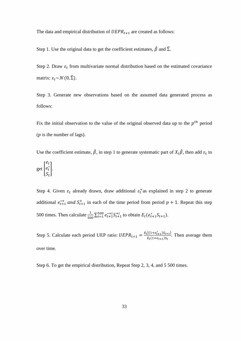
The data and empirical distribution of are created as follows:

Step 1. Use the original data to get the coefficient estimates, and .

Step 2. Draw from multivariate normal distribution based on the estimated covariance

matrix: .

Step 3. Generate new observations based on the assumed data generated process as

follows:

Fix the initial observation to the value of the original observed data up to the period

( is the number of lags).

Use the coefficient estimate, , in step 1 to generate systematic part of , then add to

get

.

Step 4. Given already drawn, draw additional as explained in step 2 to generate

additional

in each of the time period from period . Repeat this step

500 times. Then calculate

to obtain .

Step 5. Calculate each period UEP ratio:

. Then average them

over time.

Step 6. To get the empirical distribution, Repeat Step 2, 3, 4, and 5 500 times.

34

In the same fashion, to test the UIP relation, the VAR representation (3.5) is also

assumed, but

instead. The data and empirical distribution of are

similarly created as follows:



matrix: .

Step 3. Generate new observations based on the assumed data generated process as follows:




get

.

Step 4. Calculate each period UEP ratio:

. Then average them over time.

Step 5. To get the empirical distribution, Repeat Step 2, 3 and 4 500 times.

Above we elaborated how we obtain the empirical distributions and calculate the UEP ratio

and UIP ratio directly from the definitions. However, since most studies use the regression

models to test the parities, we would like to see how the regressions perform in our alternative

testing method. , we translate the regressions into the Ratios by calculating the UEP Ratio and

UIP Ratio implied by the regressions as follows.

35

UEP Ratio implied by regression

Consider the UEP regression:

, (3.6)

or .

,

where, is the UEP ratio.

,

where,

.

,

where,

. and are the Jensen’s Inequality terms.

.

.

. (3.7)

36

Simulation Method



matrix: .


follows:




get

.

Step 4. Run the UIP regression to estimate .

Step 5. Calculate each period UEP Ratio implied by regression:

, the covariance term , the Jensen’s Inequality terms

, , and . Then average them over time.

Step 6. To get the empirical distribution, Repeat Step 2, 3, 4, and 5 500 times.

UIP Ratio implied by the regression

Consider UIP regression:

, (3.8)

37

or .

,

where is the UIP Ratio.

.

,

where the Jensen’s Inequality term .

.

. (3.9)

Simulation Method



matrix: .


follows:



38


get

.

Step 4. Run the UIP regression to estimate .

Step 5. Calculate each period UEP deviation: . Then

average them over time.

Step 6. To get the empirical distribution, Repeat Steps 2, 3, 4, and 5 500 times.

3.3 Results

3.3.1 Data

The data in this empirical investigation are quarterly data on exchange rates and equity

price index in nine countries with developed financial markets over the third quarter of 1997

through the first quarter of 2007. The exchange rate in each country is the price of each

currency in terms of US dollars.13

3.3.2 UEP vs. UIP

Table 3.1 shows the central tendency of the UIP Ratio, UEP Ratio, and their standard

deviations. The central tendency of the UIP Ratio is just slightly different from unity for

every country. For example, the central tendency of the UIP Ratio for Australia is 1.002

indicating that the return from Australian (foreign) assets is just 0.2 percent higher than the

13 The data on daily spot exchange rates are from the Datastream of the WM Company/Reuters, except the euro,

which is from Barclay’s Bank International. The equity price index data are from the Datastream.

39

return from U.S. (home) assets. In other words, UIP holds better than we thought, given the

negative coefficient estimate in the UIP regression or the UIP puzzle often found in the

literature. In addition, it is surprising that the central tendency of the UIP Ratio is

significantly less than the central tendency of the UEP Ratio for every country. So, we find

that UIP holds better than UEP. This notion is opposite from the literature that mostly finds

evidence supporting UEP not UIP. However, it is not clear whether the equity carry trade is

riskier than the currency carry trade since, unlike others, the standard deviations of UIP Ratio

for Denmark, New Zealand, and Switzerland are greater than those of UEP Ratio.

Table 3.1: UIP Ratio and UEP Ratio

Country UIPR

(1)

UIPR C.I.

(2)

UIPR Std

(3)

UEPR

(4)

UEPR C.I.

(5)

UEPR Std

(6)

Australia 1.002 (1.000, 1.004) 0.025 1.060 (1.056, 1.064) 0.046

Canada 1.018 (1.013, 1.023) 0.055 1.122 (1.116, 1.129) 0.075

Denmark 1.057 (1.049, 1.065) 0.091 1.156 (1.150, 1.161) 0.064

Euro 1.008 (1.004, 1.012) 0.045 1.179 (1.173, 1.185) 0.067

Japan 0.995 (0.993, 0.997) 0.023 1.034 (1.030, 1.038) 0.049

New Zealand 1.017 (1.011, 1.023) 0.071 1.044 (1.040, 1.047) 0.040

Norway 1.038 (1.032, 1.044) 0.067 1.156 (1.150, 1.162) 0.067

Sweden 1.034 (1.028, 1.039) 0.061 1.194 (1.188, 1.200) 0.065

Switzerland 1.036 (1.029, 1.042) 0.074 1.053 (1.050, 1.056) 0.037

United Kingdom 0.987 (0.984, 0.990) 0.038 1.105 (1.101, 1.109) 0.045

Note: 1. Columns 1 and 2 show the mean of the UIP Ratio and its 95% confidence interval.

2. Column 3 shows the standard deviation of the UIP Ratio.

3. Columns 4 and 5 show the mean of the UEP Ratio and its 95% confidence interval.

4. Column 6 shows the standard deviation of the UEP Ratio

40

Why do we find such contrasting results from the literature? Most researchers employ the

UIP regression to test the UIP relation and the UEP regression to test the UEP relation.

However, when the relations do not hold, the testing does not intuitively give the magnitude

of the deviation of the relations. So, one of the benefits of using the UIP Ratio and UEP Ratio

is that this testing can tell the degree of the deviation from the parities.

Figure 3.1 illustrates the empirical distributions of the UIP Ratio and UEP Ratio

corresponding to the results in Table 3.1. Most empirical distributions are normally

distributed except those of the UIP Ratio for Denmark, Norway, Sweden, and Switzerland

which are bimodally distributed. For these countries, their interest rates fluctuate around U.S.

interest rate, so the returns of currency carry trade alternate between positive and negative.

Since most of the literature relies on the regression methods to test the parities, we are

interested to compare and contrast the UIP Ratio and UIP Ratio implied by the regressions

from the Ratios calculated directly from the definitions. Table 3.2 shows the central tendency

of the UIP Ratio, UIP Ratio implied by the regression, and the Jensen’s Inequality term. It is

clear that the central tendencies of the UIP Ratio and UIP Ratio implied by the regression are

similar. Regarding the Jensen’s Inequality term which is always left out from the regression,

the central tendency of its exponential is near unity. In other words, the Jensen’s Inequality

term is close to zero for each country. So we have the impression that the UIP regression can

be an unbiased predictor of the UIP relation.

41

Table 3.2: UIP Ratio Implied by the Regression

Country UIPR

(1)

UIPR C.I.

(2)

UIPR by

regress

(3)

UIPR by

regress C.I.

(4)

(5)

C.I.

(6)

Australia 1.002 (1.000, 1.004) 0.996 (0.994, 0.998) 1.006 (1.005, 1.006)

Canada 1.018 (1.013, 1.023) 1.015 (1.010, 1.020) 1.003 (1.003, 1.004)

Denmark 1.057 (1.049, 1.065) 1.049 (1.041, 1.057) 1.007 (1.007, 1.008)

Euro 1.008 (1.004, 1.012) 1.002 (0.998, 1.006) 1.007 (1.006, 1.007)

Japan 0.995 (0.993, 0.997) 0.992 (0.990, 0.994) 1.004 (1.003, 1.004)

New Zealand 1.017 (1.011, 1.023) 1.001 (0.996, 1.006) 1.013 (1.013, 1.014)

Norway 1.038 (1.032, 1.044) 1.031 (1.026, 1.037) 1.006 (1.006, 1.007)

Sweden 1.034 (1.028, 1.039) 1.027 (1.021, 1.032) 1.007 (1.006, 1.007)

Switzerland 1.036 (1.029, 1.042) 1.029 (1.023, 1.036) 1.006 (1.006, 1.007)

United Kingdom 0.987 (0.984, 0.990) 0.985 (0.982, 0.989) 1.002 (1.001, 1.002)

Note: 1. Columns 1 and 2 show the mean of the UIP Ratio calculated directly from the definition and its 95%

confidence interval.

2. Columns 2 and 3 show the mean of the UIP Ratio implied by the regression and its 95% confidence

interval.

3. Columns 5 and 6 show the central tendency of exponential of the Jensen’s Inequality term and its

95% confidence interval.

Figure A3.2 illustrates the empirical distribution of the UIP Ratio implied by the

regressions and exponential of the Jensen’s Inequality Term corresponding to results in Table

3.2. Most empirical distributions are normally distributed except those of the UIP Ratio for

Denmark, Norway, Sweden, and Switzerland which are bimodally distributed. For these

countries, their interest rates fluctuate around the U.S. interest rate, so the returns of currency

carry trade alternate between positive and negative.

Similarly, we contrast the UEP Ratio and UEP Ratio implied by the regressions from the

Ratios calculated directly from the definitions. Table 3.3 shows the central tendency of the

UEP Ratio, UEP Ratio implied by the regression, the covariance of foreign equity return and

exchange rate, and the Jensen’s Inequality terms. By comparing columns 1 and 3, we find

42

that the UEP Ratio implied by the regression is significantly less than the UEP Ratio

calculated directly from the definition. This suggests that the UEP regression is a bias

predictor of the UEP relation. In order to investigate where the bias is from, we calculate the

terms that are usually left out from the regression: the covariance of foreign equity return and

exchange rate, and the Jensen’s Inequality terms. Columns 5, 7, 9 and 11 show the central

tendency of the exponential of the covariance term and Jensen’s Inequality terms,

respectively. We find that the covariance term is far from zero (its exponential is far from

unity). However, the Jensen’s Inequality terms are relatively small and close to zero. Now we

have the impression that the bias from the UEP regression comes from the ignorance of the

covariance term. The positive covariance term suggests that when the foreign equity return

increases, demand of the foreign currency rises making the foreign currency appreciate. This

is why the expected foreign equity return is greater than the expected domestic equity return

in our model.

Figure A3.3 shows empirical distributions of the UEP Ratio implied by the regression,

exponentials of the covariance term and the Jensen’s Inequality terms. All empirical

distributions are normally distributed.

43

Table 3.3: UEP Ratio Implied by the Regression Country UEPR

(1)

UEPR C.I.

(2)

UEPR by

regress

(3)

UEPR by

regress C.I.

(4)

(5)

C.I.

(6)

Australia 1.060 (1.056, 1.064) 1.012 (1.007, 1.017) 1.046 (1.044, 1.047)

Canada 1.122 (1.116, 1.129) 1.029 (1.022, 1.036) 1.089 (1.086, 1.091)

Denmark 1.156 (1.150, 1.161) 1.043 (1.036, 1.051) 1.107 (1.103, 1.111)

Euro 1.179 (1.173, 1.185) 1.043 (1.036, 1.051) 1.134 (1.129, 1.140)

Japan 1.034 (1.030, 1.038) 1.013 (1.008, 1.017) 1.020 (1.019, 1.022)

New Zealand 1.044 (1.040, 1.047) 1.028 (1.024, 1.033) 1.012 (1.011, 1.013)

Norway 1.156 (1.150, 1.162) 1.039 (1.032, 1.046) 1.111 (1.107, 1.115)

Sweden 1.194 (1.188, 1.200) 1.041 (1.035, 1.048) 1.147 (1.141, 1.152)

Switzerland 1.053 (1.050, 1.056) 1.001 (0.996, 1.006) 1.053 (1.050, 1.055)

United

Kingdom 1.105 (1.101, 1.109) 1.008 (1.003, 1.013) 1.097 (1.094, 1.101)

Table 3.3: UEP Ratio Implied by the Regression (Continued) Country

(7)

exp C.I.

(8)

(9)

C.I.

(10)

(11)

C.I.

(12)

Australia 1.010 (1.009, 1.011) 1.004 (1.003, 1.005) 1.010 (1.008, 1.011)

Canada 0.996 (0.995, 0.997) 1.014 (1.012, 1.016) 1.007 (1.006, 1.009)

Denmark 0.998 (0.997, 0.999) 1.019 (1.016, 1.021) 1.013 (1.011, 1.015)

Euro 0.978 (0.976, 0.980) 1.033 (1.030, 1.037) 1.010 (1.008, 1.012)

Japan 0.997 (0.996, 0.999) 1.010 (1.009, 1.012) 1.003 (1.002, 1.004)

New Zealand 1.006 (1.005, 1.006) 1.002 (1.001, 1.002) 1.004 (1.003, 1.005)

Norway 0.984 (0.982, 0.985) 1.028 (1.025, 1.031) 1.008 (1.007, 1.010)

Sweden 0.964 (0.962, 0.967) 1.050 (1.046, 1.053) 1.014 (1.012, 1.015)

Switzerland 1.001 (1.000, 1.002) 1.008 (1.006, 1.010) 1.007 (1.006, 1.009)

United

Kingdom 0.999 (0.999, 1.000) 1.020 (1.018, 1.023) 1.017 (1.015, 1.020)

44

Note: 1. Columns 1 and 2 show the mean of the UEP Ratio calculated directly from the definition and its

95% confidence interval.

2. Columns 2 and 3 show the mean of the UEP Ratio implied by the regression and its 95% confidence

interval.

3. Columns 5 and 6 show the central tendency of exponential of

and its 95% confidence interval.

4. Columns 7 and 8 show the central tendency of exponential of the Jensen’s Inequality term and its 95% confidence interval.

5. Columns 9 and 10 show the central tendency of exponential of the Jensen’s Inequality term


6. Columns 11 and 12 show the central tendency of exponential of the Jensen’s Inequality term


45

3.4 Conclusion

The UIP regression has long been used to test the UIP relation. Recently, Hau and Rey

(2006), Cappiello and De Santis (2005), and Kim (2011) modify the UIP regression to

replace the returns from risk-free assets such as T-bills with the expected returns from risky

assets such as equity. It is called the UEP regression, and it has been used to test the UEP

relation, an arbitrage condition in equity markets. In this paper, we find problems with the

regression method used to test the existence of the parities. First, the regression method does

not intuitively give the magnitude of deviation when the UIP or UEP relation does not hold.

In addition, the UEP relation should be hold ex-ante not ex-post. However, the expected

equity returns are not known ex ante. If ex-post data are used in the UEP regression [as done

by Hau and Rey (2006), Cappiello and De Santis (2005), and Kim (2011)], the regression is

not valid

Due to the shortcomings of the regression method, we propose an alternative method to

test the UIP relation and UEP relation called the UIP Ratio and UEP Ratio, respectively, by

the simulation technique. We come up with four main findings. First, UIP is less puzzling

than we thought since the UIP regression does not intuitively give the magnitude of the

deviation in UIP. Second, unlike the literature, we find that UIP holds better than UEP. Third,

the UEP regression is a bias predictor of the deviation in UEP because the covariance of

foreign equity return and exchange rate is left out. Finally, the expected foreign equity return

is greater than the expected domestic equity return in our model. The reason is that

is positive ( . When the foreign equity return increases, demand

for the foreign currency rises making the foreign currency appreciate.

46

Chapter 4

Summary

Uncovered interest parity (UIP) is a no-arbitrage condition in the asset market where

trades are instantaneous and virtually frictionless. UIP explains an equilibrium in which a

speculator is indifferent between interest bearing identical assets denominated in different

currency. UIP predicts that a high interest currency tends to depreciate against a low interest

rate currency by the same percentage point as the interest rate differential between the two

countries. Empirically, when the exchange rate change is regressed on the interest rate

differential the null hypothesis that the slope coefficient is unity should not be rejected.

It is important to emphasize that empirically, the exchange rate change can be predicted

by not only the interest rate differential but also the inflation differential via the relative PPP

relation. Relative PPP is an equilibrium in the goods market. Relative PPP predicts that a

high-inflation currency tends to depreciate against a low-inflation currency. To test relative

PPP, the exchange rate change is regressed on the inflation differential. Therefore, it is

crucial to distinguish whether the exchange rate change is due to the asset market (UIP

relation) or goods market (relative PPP relation).

It has long been known that the uncovered interest parity (UIP) relation rarely holds

empirically. Most studies use the data from developed economies and find that the UIP slope

coefficient is often not only less than unity but also negative. However, when data from

emerging economies are used, the UIP slope coefficient is not negative (though still far from

unity). In other worlds, according to these findings, the UIP relation is less puzzling for

emerging economies. In this dissertation, we attempt to answer the following question: are

47

the economies of developing countries different from those of developed countries in the

context of the UIP condition?

In Chapter 2, we find that low inflation countries (most are developed countries) and high

inflation countries (all are developing countries) are different in context of nominal UIP. That

is, the “nominal UIP puzzle” is less prevalent in high inflation countries than in low inflation

countries. However, regarding the real UIP relation, the two groups of countries are similar.

Specifically, the low inflation countries have the same degree of “real UIP puzzle” as the

high inflation countries. This is the broad contribution of Chapter 2. We argue that the

exchange rate change in high-inflation countries is due to the relative PPP relation, not the

UIP relation as in low-inflation countries. It appears that the inflation plays a role of a noise

in rather than a key to unlock the puzzle underlying the UIP relation. If this is the case, future

research should focus on the real UIP relation. In addition, more research should investigate

and explain the “real UIP puzzle.”

With increases in financial globalization, investors hold foreign risk-free assets or bonds

as well as risky-assets such as equities. The increasing portion of international equity flows

and the notorious empirical failure of UIP are motivations to explore an alternative no-

arbitrage condition in which, instead of interest rate differential, expected equity return

differential between two countries is equal to expected change in exchange rate, called the

“uncovered equity parity” (UEP) condition. UEP states that when expected foreign equity

return is higher than the expected U.S. equity return, rational and risk-neutral U.S. investors

should expect the foreign currency to depreciate against the dollar by the difference between

the two expected returns. In the literature, UEP is largely supported by data in the sense that

equity return differential predicts exchange rate movement in the right direction. This

suggests that UEP holds better than UIP.

48

In Chapter 3, we find problems with the regression method used to test the UIP or UEP

relation. First, the regression method does not intuitively give the magnitude of deviation

when the UIP or UEP relation does not hold. In addition, the UEP relation should be hold ex-

ante not ex-post. However, the expected equity returns are not known ex ante. We propose an

alternative method to test UIP and UEP. This is the broad contribution of Chapter 3. Our

method intuitively gives the magnitude of the deviation from the parities. With shortcomings

of conventional UIP and UEP testing using the regressions, we find that UIP actually holds

better than UEP. Furthermore, we find that the UEP regression is a bias predictor of the

deviation in UEP because the covariance of foreign equity return and exchange rate is left

out. In future research, we should investigate why the arbitrage in the assets market via UIP

holds better than the arbitrage in the equity markets via UEP.

49

References

Alvarez, Fernando, Andrew Atkeson and Patrick J. Kehoe (2005) “Time-Varying Risk,

Interest Rates, and Exchange Rates in General Equilibrium,” Staff Report, Federal

Reserve Bank of Minneapolis.

Bacchetta, Philippe and Eric van Wincoop (2005) “Rational Inattention: a Solution to the

Forward Discount Puzzle,” NBER Working Paper 11633.

Bacchetta, Philippe and Eric van Wincoop (2009) “Infrequent Portfolio Decisions: a Solution

to the Forward Discount Puzzle,” Forthcoming, American Economics Review.

Bansal, R. and Dahlquist, M. (2000) “The Forward Premium Puzzle: Different Tales from

Developed and Emerging Economies,” Journal of International Economics 51: 115–

144.

Burnside, Craig, Martin Eichenbaum and Sergio Rebelo (2007) “The Returns to Currency

Speculation in Emerging Markets,” NBER Working Paper 12916.

Burnside, Craig, Martin Eichenbaum, Isaac Kleshchelski and Sergio Rebelo (2006) “The

Returns to Currency Speculation,” NBER Working Paper 12489.

______(2008). “Do Peso Problems Explain the Returns to the Carry Trade?,” NBER

Working Paper 14054.

Cappiello, Lorenzo, and Roberto A. De Santis (2005) “Explaining the Exchange Rate

Dynamic the Uncovered Equity Return Parity Condition,” ECB Working Paper No.

529.

Cappiello, Lorenzo, and Roberto A. De Santis (2007) “The Uncovered Equity Return Parity

Condition,” ECB Working Paper No. 812.

Curcuru, Stephanie E., Charles P. Thomas, Francis E. Warnock, and Jon Wongswan (2014)

“Uncovered Equity Parity and Rebalancing in International Portfolios,” NBER

Working Paper 19963

50

Engle, Charles (1996) “The Forward Discount Anomaly and the Risk Premium: a Survey of

Recent Evidence,” Journal of Empirical Finance 3: 123-192.

______(2011) “The Real Exchange Rate, Real Interest Rates, and the Risk Premium,” NBER

Working Paper 17116.

Engle, Charles and Anthony P. Rodrigues (1989) “Tests of International CAPM with Time-

Varying Covariances,” Journal of Applied Econometrics, 4: 119-38.

Engle, Charles and Jeffrey Frankel. (1984) “Do Asset Demand Functions Optimize over the

Mean and Variance of Real Returns? A Six-Currency Test,” Journal of International

Economics 17: 309-323.

Evans, Martin D. D. and Karen K. Lewis (1995) “Do Long-Term Swings in the Dollar Affect

Estimates of the Risk Premia?,” Review of Financial Studies, 8: 709-42.

Fama, E. F (1984). “Forward and Spot Exchange Rates,” Journal of Monetary Economics,

14, 319-38.

Flood, R. and Rose, A. (2002) “Uncovered interest parity in crisis.” IMF Staff Papers 49(2):

252–266.

Frankel, Jeffrey and Jumana Poonawala (2006) “The Forward Market in Emerging

Currencies: Less Biased Than in Major Currencies,” NBER Working Paper 12496.

Gilmore, Stephen and Fumio Hayashi (2008) “Emerging Market Currency Excess Returns”

NBER Working Paper 14528.

Hau, Harald, and Helene Rey (2006) “Exchange Rates, Equity Prices, and Capital Flows,”

The Review of Financial Studies19: 273-317.

Kim, Heeho (2011) “The Risk Adjusted Uncovered Equity Parity,” Journal of International

Money and Finance 30: 1491-1505.

Lucas, R.E. Jr., (1982) “Interest Rates and Currency Prices in a Two-Country World,”

Journal of Monetary Economics 10: 335-359.

51

Lustig, H. and Verdelhan, A. (2007) “The Cross Section of Foreign Currency Risk Premia

and Consumption Growth Risk,” American Economic Review 97(1): 89–117.

Mark, Nelson C. (1988) “Time Varying Betas and Risk Premia in the Pricing of Forward

Foreign Exchange Contracts," Journal of Financial Economics 22: 335-354.

Stock, James H. and Mark W. Watson (1999) “Forecasting Inflation,” Journal of Monetary

Economics 44: 293-335.

52

Appendix

Table A 2.1: Country Information

ID Country Start

Date

End

Date

Inflation

Group

Interest Rate

Source

Unemployment Rate

Source

1 Argentina 1997q4 2009q1 H DS -

2 Australia 1997q3 2009q1 L DS OECD

3 Austria 1994q1 1998q4 L DS OECD

4 Belgium 1994q1 1998q4 L DS OECD

5 Brazil 2000q1 2009q1 H GFD OECD

6 Canada 1994q1 2009q1 L DS OECD

7 Colombia 2001q3 2008q1 H GFD IMF

8 Croatia 1997q4 2006q2 H DS -

9 Czech Republic 1995q2 2009q1 H DS OECD

10 Denmark 1994q1 2009q1 L DS -

11 Eurozone 1999q2 2009q1 L DS OECD

12 Finland 1994q1 1998q4 L DS OECD

13 France 1994q1 1998q4 L DS OECD

14 Germany 1994q1 1998q4 L DS OECD

15 Greece 1994q4 2000q4 H DS -

16 Hong Kong 1997q3 2009q1 L DS IMF

17 Hungary 1996q1 2009q1 H DS OECD

18 Iceland 1998q4 2007q4 H DS -

19 India 1999q3 2009q1 H DS -

20 Indonesia 1997q3 2009q1 H GFD -

21 Ireland 1994q1 1998q4 L DS OECD

22 Italy 1994q1 1998q4 L DS OECD

23 Japan 1994q1 2009q1 L DS OECD

24 Mexico 2001q4 2009q1 H DS OECD

25 Netherlands 1994q1 1998q4 L DS -

26 New Zealand 1997q3 2009q1 L DS OECD

27 Norway 1994q1 2009q1 L DS OECD

28 Pakistan 1994q2 2009q1 H DS -

29 Philippines 1999q4 2006q3 H DS IMF

30 Poland 1994q2 2009q1 H DS OECD

31 Portugal 1994q1 1998q4 L DS IMF

32 Romania 1997q3 2009q1 H DS -

33 Russia 1996q3 2009q1 H DS -

34 Singapore 1994q1 2009q1 L DS -

35 Slovakia 1997q3 2008q4 H DS OECD

36 South Africa 1997q3 2009q1 H DS -

37 Spain 1994q1 1998q4 L DS OECD

38 Sweden 1997q3 2009q1 L DS OECD

39 Switzerland 1994q1 2009q1 L BBA OECD

40 Thailand 1997q3 2006q3 H DS -

41 Turkey 2003q1 2009q1 H DS OECD

42 United Kingdom 1994q1 2009q1 L DS OECD

Note: L and H indicate low and high inflation countries, respectively. DS, GFD and BBA stand for the

Datastream, the Global Financial Data and the British Bankers’ Association, respectively. IMF data

was obtained from the International Monetary Fund’s International Financial Statistics CD released for

June 2009. OECD data was retrieved from http://stats.oecd.org/.

http://stats.oecd.org/

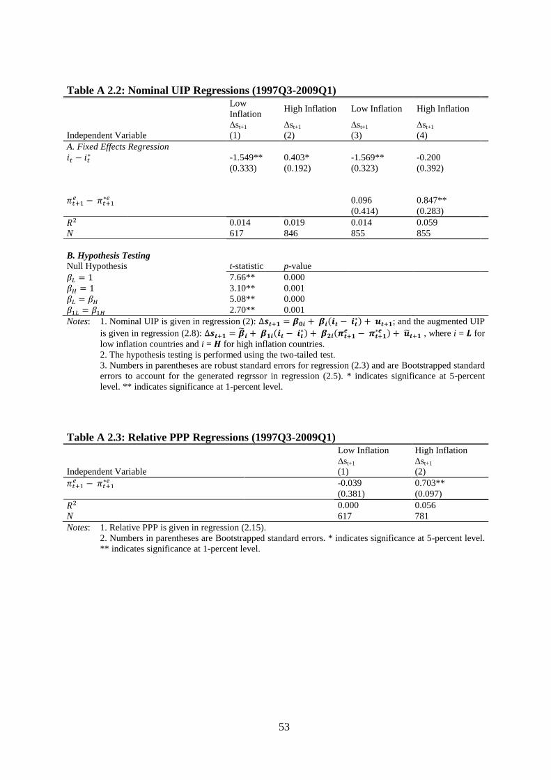
53

Table A 2.2: Nominal UIP Regressions (1997Q3-2009Q1)

Low

Inflation High Inflation Low Inflation High Inflation

∆st+1 ∆st+1 ∆st+1 ∆st+1



-1.549** 0.403* -1.569** -0.200

(0.333) (0.192) (0.323) (0.392)

0.096 0.847**

(0.414) (0.283)

0.014 0.019 0.014 0.059

N 617 846 855 855



7.66** 0.000

3.10** 0.001

5.08** 0.000

2.70** 0.001

Notes: 1. Nominal UIP is given in regression (2): ; and the augmented UIP


, where i = for



3. Numbers in parentheses are robust standard errors for regression (2.3) and are Bootstrapped standard



Table A 2.3: Relative PPP Regressions (1997Q3-2009Q1) Low Inflation High Inflation

∆st+1 ∆st+1


-0.039 0.703**

(0.381) (0.097)

0.000 0.056

N 617 781




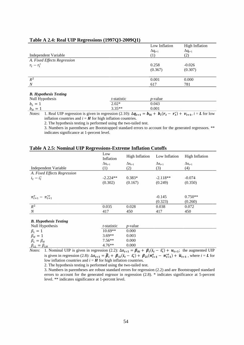
54

Table A 2.4: Real UIP Regressions (1997Q3-2009Q1)

Notes: 1. Real UIP regression is given in regression (2.10): , i = for low

inflation countries and i = for high inflation countries.



indicates significance at 1-percent level.

Table A 2.5: Nominal UIP Regressions-Extreme Inflation Cutoffs

Low

Inflation High Inflation Low Inflation High Inflation

∆st+1 ∆st+1 ∆st+1 ∆st+1



-2.224** 0.383* -2.118** -0.074

(0.302) (0.167) (0.249) (0.350)

-0.145 0.750**

(0.323) (0.260)

0.035 0.028 0.038 0.072

N 417 450 417 450



10.69** 0.000

3.69** 0.003

7.56** 0.000

4.76** 0.000

Notes: 1. Nominal UIP is given in regression (2.2): ; the augmented UIP


, where i = for



3. Numbers in parentheses are robust standard errors for regression (2.2) and are Bootstrapped standard




∆qt+1 ∆qt+1



0.258 -0.026

(0.367) (0.307)

0.001 0.000

N 617 781



2.02* 0.043

3.35** 0.001

55

Table A 2.6: Relative PPP Regressions-Extreme Inflation Cutoffs Low Inflation High Inflation

∆st+1 ∆st+1


-0.619 0.692**

(0.321) (0.111)

0.007 0.071

N 397 450




3. Low Inflation is lower than the 1st quartile; High Inflation is greater than the 3

rd quartile.

Table A 2.7: Real UIP Regressions-Extreme Inflation Cutoffs

Notes: 1. Real UIP regression is given in regression (2.10): , i = for low

inflation countries and i = for high inflation countries.



indicates significance at 1-percent level.

4. Low Inflation is lower than the 1st quartile; High Inflation is greater than the 3

rd quartile.


∆qt+1 ∆qt+1



0.574 0.019

(0.271) (0.286)

0.007 0.000

N 397 450



1.57 0.117

3.43** 0.001

56

Figure A3.1: Distribution of the UIP Ratio (left) and UEP Ratio (right)

A. Australia

B. Canada

C. Denmark

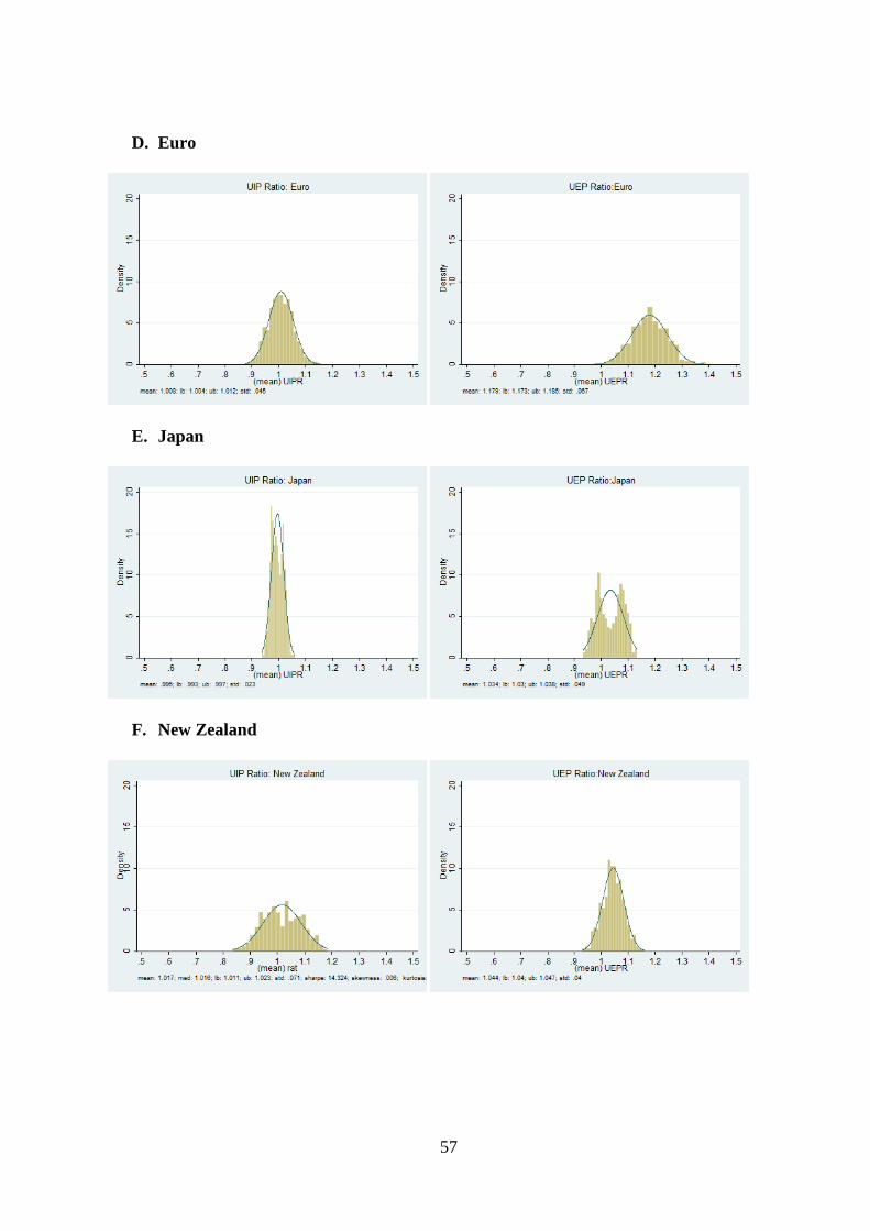
57

D. Euro

E. Japan

F. New Zealand

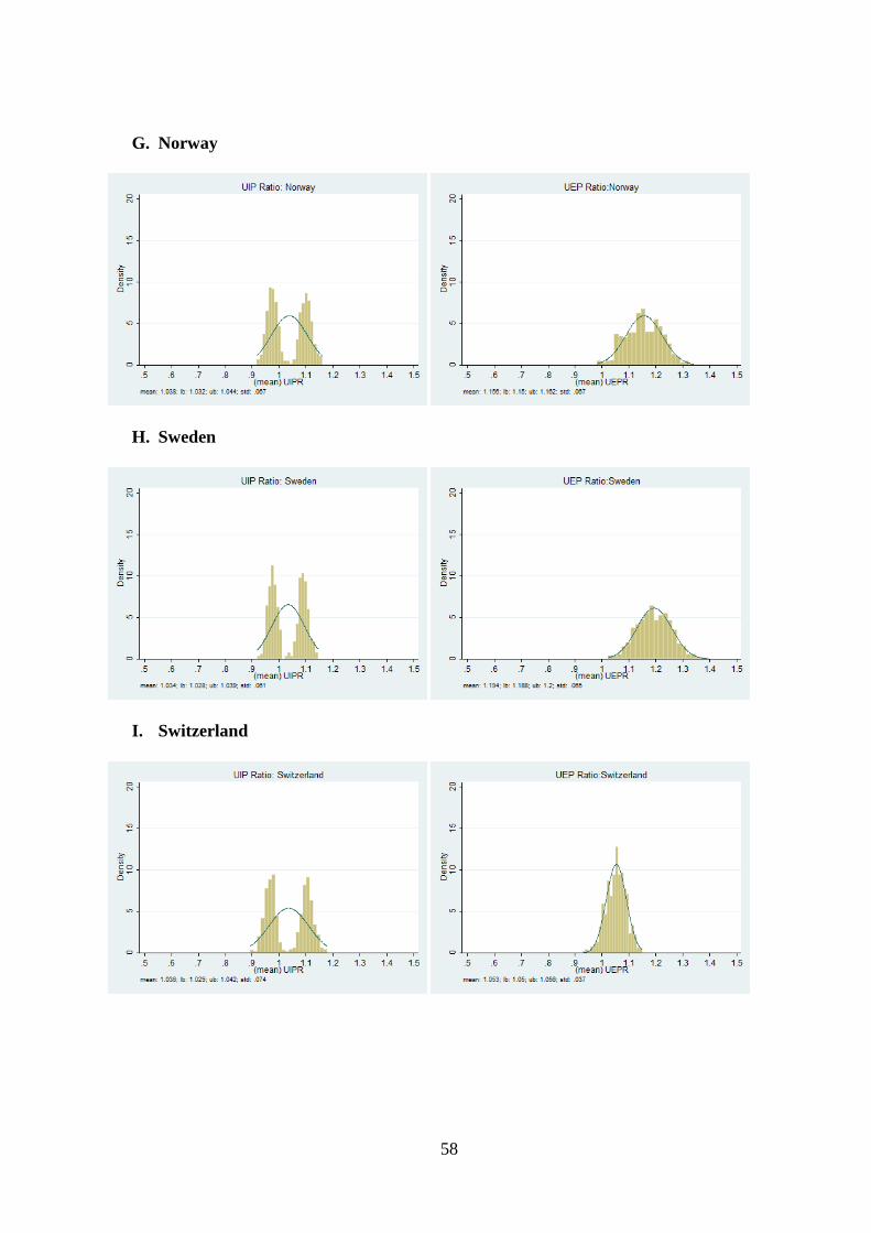
58

G. Norway

H. Sweden

I. Switzerland

59

J. United Kingdom

60

Figure A3.2: Empirical Distribution of the UIP Ratio implied by the regressions (left)

and exponential of the Jensen’s Inequality Term (right)

A. Australia

B. Canada

C. Denmark

61

D. Euro

E. Japan

F. New Zealand

62

G. Norway

H. Sweden

I. Swtizerland

63

J. United Kingdom

64

Figure A3.3: Empirical Distributions of the UEP Ratio implied by the regression,

exponential of the covariance term, and exponential of the Jensen’s Inequality terms

A. Australia

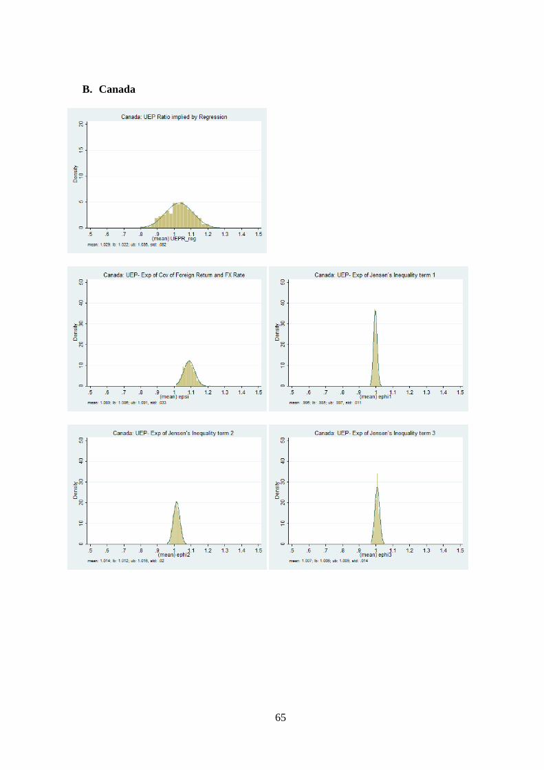
65

B. Canada

66

C. Denmark

67

D. Euro

68

E. Japan

69

F. New Zealand

70

G. Norway

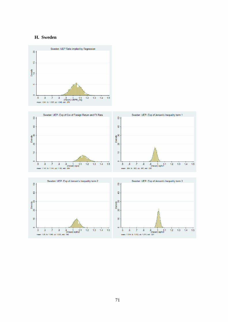
71

H. Sweden

72

I. Switzerland

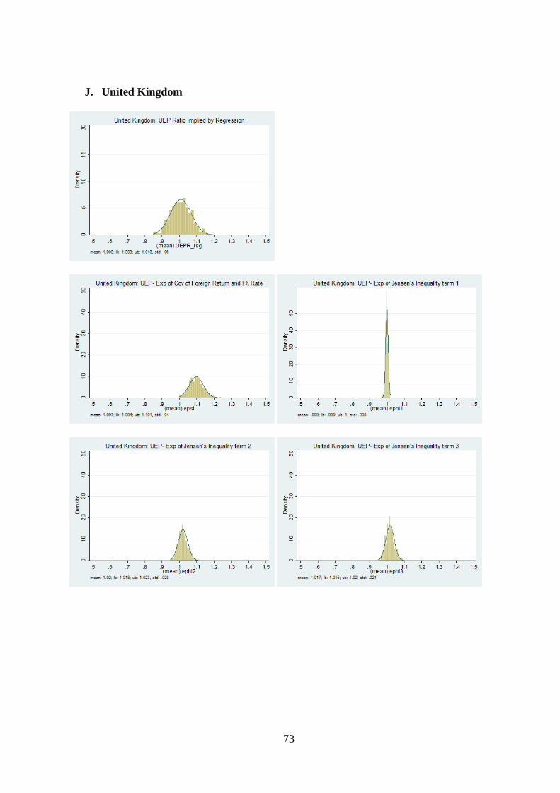
73

J. United Kingdom

Documents

Forward Premium Puzzle