Embed Size (px)
Citation preview
Fossil Fuel Producing Economies have Greater
Potential for Interfuel Substitution
By
Jevgenijs Steinbuks and
Badri G. Narayanan
GTAP Working Paper No. 73
2014
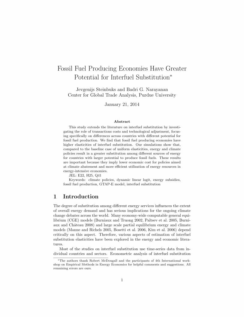
Fossil Fuel Producing Economies Have Greater
Potential for Interfuel Substitution∗
Jevgenijs Steinbuks and Badri G. NarayananCenter for Global Trade Analysis, Purdue University
January 21, 2014
Abstract
This study extends the literature on interfuel substitution by investi-gating the role of transactions costs and technological adjustment, focus-ing specifically on differences across countries with different potential forfossil fuel production. We find that fossil fuel producing economies havehigher elasticities of interfuel substitution. Our simulations show that,compared to the baseline case of uniform elasticities, energy and climatepolicies result in a greater substitution among different sources of energyfor countries with larger potential to produce fossil fuels. These resultsare important because they imply lower economic cost for policies aimedat climate abatement and more efficient utilization of energy resources inenergy-intensive economies.
JEL: E22, H25, Q41Keywords: climate policies, dynamic linear logit, energy subsidies,
fossil fuel production, GTAP-E model, interfuel substitution
1 Introduction
The degree of substitution among different energy services influences the extentof overall energy demand and has serious implications for the ongoing climatechange debates across the world. Many economy-wide computable general equi-librium (CGE) models (Burniaux and Truong 2002, Paltsev et al. 2005, Burni-aux and Chateau 2008) and large scale partial equilibrium energy and climatemodels (Manne and Richels 2005, Bosetti et al. 2006, Kim et al. 2006) dependcritically on this aspect. Therefore, various aspects of estimation of interfuelsubstitution elasticities have been explored in the energy and economic litera-tures.
Most of the studies on interfuel substitution use time-series data from in-dividual countries and sectors. Econometric analysis of interfuel substitution
∗The authors thank Robert McDougall and the participants of 4th International work-shop on Empirical Methods in Energy Economics for helpful comments and suggestions. Allremaining errors are ours.
1
using international cross-country and cross-sector data was until recently re-stricted to a handful of studies focusing mainly on G7 economies (Pindyck 1979,Jones 1996, Renou-Maissant 1999). Several recent studies estimated interfuelsubstitution elasticities using aggregate and sector level data for a number ofcountries (Serletis et al. 2010b, 2011). In these (and earlier) studies, the demandfor fuels is modeled as a function of input prices and output following standardderivations based on economic theory.
This paper extends the existing literature on interfuel substitution in aninternational context by investigating the role of non-price factors, focusingspecifically on international fuel production. The economic literature makestwo arguments as to why the extent of interfuel substitution may differ acrossthe fossil fuel producing and non-producing economies. First, transaction (e.g.,transportation, storage, and import clearance) costs and differences in fuel char-acteristics (e.g., energy and carbon content) render domestically produced fuelsto be imperfect substitutes for foreign commodities (Armington 1969). If thisis the case, the degree of interfuel substitution will be higher in the fossil fuelproducing economies. For example, in the presence of low production (i.e., ex-traction) and high transactions costs, domestically produced coal will be ableto compete against imported oil and natural gas, whereas imported coal won’t.Several recent studies attempted to estimate Armington elasticities of substitu-tion for different fuels. The size of estimated elasticities was drastically differentacross these studies, starting from close to zero (Welsch 2008) to above twenty(Balistreri et al. 2010). These studies use different data and econometric meth-ods, and their results are difficult to reconcile.
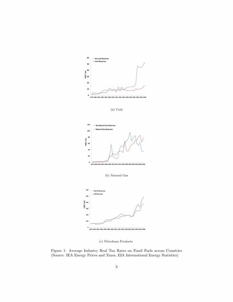
Second, many resource-rich countries have historically subsidized the pro-duction of their energy resources for the purposes of economic stimulation, en-hanced trade performance, inflation control, and energy security (Kosmo 1987).According to International Energy Agency (IEA) estimates, total subsidies tofossil fuel consumption in 37 non-OECD countries amounted in 2008 to USD 557billions, almost five times the yearly bilateral aid flows to developing countriesin the form of Official Development Assistance (Burniaux and Chateau 2011).Figure 1 demonstrates that only in the recent years fuel consumption taxes inoil and natural gas-rich countries converged to (and even exceeded) the levelsof countries with no natural resources.1 And the taxes on coal consumptionare still considerably lower in coal-rich economies. Kosmo (1987) demonstratedthat such policies encourage over-investment in energy-intensive industries atthe expense of other sectors. Heavy capital investment in a particular fuel-using sector will mean difficulties in shifting to another fuel sector in short andmedium run because switching to alternative fuels are not always technologi-cally feasible (Steinbuks 2012) or are too costly to implement (Jacoby and Wing1999). Combined with organizational barriers to technology adoption, boundedrationality, and information asymmetries, energy subsidies may result in an en-ergy and carbon “lock-in” (Unruh 2000), and negatively affect the degree of
1Figure 1 excludes several oil exporting countries where fossil fuel subsidies are still huge,amounting to 10% or more of GDP (Burniaux and Chateau 2011, annex II)
2
0
10
20
30
40
50
60
1978 1980 1982 1984 1986 1988 1990 1992 1994 1996 1998 2000 2002 2004 2006 2008
USD
/ t
oe
No Coal Reserves
Coal Reserves
(a) Coal
0
20
40
60
80
100
120
1978 1980 1982 1984 1986 1988 1990 1992 1994 1996 1998 2000 2002 2004 2006 2008
USD
/ t
oe
No Natural Gas Reserves
Natural Gas Reserves
(b) Natural Gas
0
100
200
300
400
500
600
1978 1980 1982 1984 1986 1988 1990 1992 1994 1996 1998 2000 2002 2004 2006 2008
USD
/ t
oe
No Oil Reserves
Oil Reserves
(c) Petroleum Products
Figure 1: Average Industry Real Tax Rates on Fossil Fuels across Countries(Source: IEA Energy Prices and Taxes, EIA International Energy Statistics)
3
interfuel substitution.To evaluate these arguments we estimate an econometric model of interfuel
substitution using a large unbalanced panel dataset of 63 countries. Based onthe model’s estimates, we calculate own-price and cross-price elasticities of fueldemand across the entire dataset, and separately across country groups basedon their potential to produce fossil fuels.
Our econometric results lend support for both arguments. For evidenceof carbon lock-in we find that countries with a potential to produce any ofthe available fossil fuels (i.e., coal, natural gas, and oil) have a considerablylonger adjustment of fuel-using capital stocks. For these, more energy-intensive,countries the share of same year response to fuels’ price change was less thanfifty percent as opposed to ninety percent in countries with no potential toproduce any fossil fuels. As a result, countries with a potential to produce anyof available fossil fuels have considerably higher difference between short andlong run elasticities of fuel substitution.
As for evidence of transaction costs argument, we find that, for most fuelpairs, the estimated elasticities of fuel substitution are considerably higher forthe countries with a potential to produce all fossil fuels or at least one fossil fuel.For example, short run cross-price elasticity of coal with respect to electricityprices (the largest in the sample) is more than four times higher for countrieswith a potential to produce any fossil fuels than for countries with no potentialto produce fossil fuels. Moreover, in many cases short run elasticities of fuelsubstitution for countries with a potential to produce fossil fuels are higher thanlong run elasticities for countries with no potential to produce fossil fuels.
To demonstrate the significance of our findings we use calculated elasticitiesto evaluate the effects of a carbon tax and reduction in oil subsidies using GTAP-E computable general equilibrium modelling framework. Our simulations showthat, compared to the baseline case of uniform elasticities of fuel substitution,carbon tax results in a greater decline in coal consumption in countries witha potential to produce fossil fuels. This happens because these countries havelarger elasticities of coal for natural gas and electricity. Our simulations alsoshow that the size of calculated elasticities affects economic response to reduc-tion in oil subsidies. Compared to the baseline case of uniform elasticities offuel substitution, the production of oil, oil products and natural gas declines,while that of coal and electricity increases by a greater amount in the countrieswith a potential to produce all fossil fuels. And production of oil and oil prod-ucts declines, and production of coal, natural gas, and electricity increases by agreater amount in countries with potential to produce one or two fossil fuels.
Our results are important in the light of recent efforts by the internationalcommunity to reduce carbon emissions (IPCC 2007) and fossil fuel subsidies(IEA et al. 2010). We find greater potential for interfuel substitution in energyintensive, fossil fuel producing economies. This implies lower economic costfor policies aimed at climate abatement and more efficient utilization of energyresources.
4
2 Model and Empirical Specification
The purpose of this section is to present an econometric model for estimat-ing parameters of fuel demand function. Ideally, such a model should explic-itly account for the adjustments of capital stocks of energy-using technologies.Dynamic structural econometric models that account for the adjustment ofenergy-using capital stocks are well established in the economic literature onenergy demand (Berndt et al. 1981, Pindyck and Rotemberg 1983, Popp 2001,Sue Wing 2008, Steinbuks and Neuhoff 2010). However, their implementationin the econometric analysis of interfuel substitution in an international contextis not possible due to data limitations on fuel-using capital. This study takesthe next available alternative, and, following previous literature, treats capitalstocks as dynamic unobserved variables.
The basic assumption underlying the econometric model is that a fuel-usingsector in each country is represented by a neo-classical agent (firm) that solvesthe cost-minimization problem. The firm’s production function requires the useof four energy inputs: coal, natural gas, petroleum products, and electricity. Itis assumed that the agent’s cost is weakly separable in energy and other (e.g.labor and capital) inputs, and the corresponding cost function is a continuous,nondecreasing, concave, and linear homogenous function of input prices. Whilethese assumptions (especially those of separability and homotheticity) are quiterestrictive, they allow us to derive conditional input demand functions for energyinputs without explicit consideration of other inputs.
The empirical model adopted in this study is the dynamic version of thelinear logit model suggested by Considine and Mount (1984) and extended byConsidine (1990), which is widely employed in the empirical literature on inter-fuel substitution (Considine 1989, Jones 1995, 1996, Urga and Walters 2003,Brannlund and Lundgren 2004, Steinbuks 2012). The advantage of this func-tional form is that it is better suited to satisfy the restrictions of economictheory and is consistent with more realistic adjustment of the unobserved cap-ital stocks to input price changes. Jones (1995) and Urga and Walters (2003)compared the predictions of the dynamic specifications of translog and linearlogit models. Both studies concluded that a linear logit specification yields morerobust results and should, therefore, be preferred in the empirical analysis ofinterfuel substitution.2
As the model is widely employed in the interfuel substitution literature,in this paper we present only main derivations, final estimating forms, andelasticity formulas. Interested reader may refer to Considine and Mount (1984)and Considine (1990) for more details. A dynamic version of the linear logitmodel can be expressed in terms of a set of non-homothetic cost shares withnon-neutral technical change as follows:
2Other recent approaches to econometric modelling of inter-fuel substitution (Serletis andShahmoradi 2008, Serletis et al. 2010a,b, 2011) use globally flexible functional forms (Fourier,AIM), as well as locally flexible (NQ, translog) functional forms. Sorting between the resultsbased on these approaches and the one adopted here is beyond the scope of this paper.
5
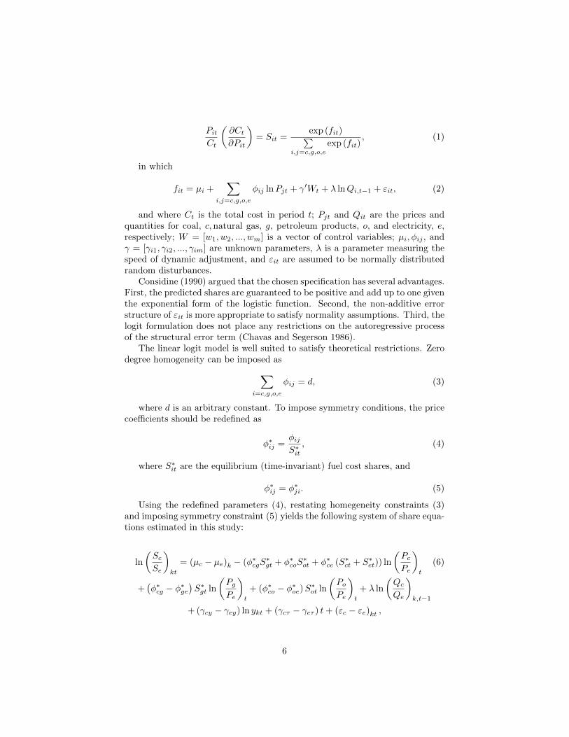
PitCt
(∂Ct∂Pit
)= Sit =
exp (fit)∑i,j=c,g,o,e
exp (fit), (1)
in which
fit = µi +∑
i,j=c,g,o,e
φij lnPjt + γ′Wt + λ lnQi,t−1 + εit, (2)
and where Ct is the total cost in period t; Pjt and Qit are the prices andquantities for coal, c,natural gas, g, petroleum products, o, and electricity, e,respectively; W = [w1, w2, ..., wm] is a vector of control variables; µi, φij , andγ = [γi1, γi2, ..., γim] are unknown parameters, λ is a parameter measuring thespeed of dynamic adjustment, and εit are assumed to be normally distributedrandom disturbances.
Considine (1990) argued that the chosen specification has several advantages.First, the predicted shares are guaranteed to be positive and add up to one giventhe exponential form of the logistic function. Second, the non-additive errorstructure of εit is more appropriate to satisfy normality assumptions. Third, thelogit formulation does not place any restrictions on the autoregressive processof the structural error term (Chavas and Segerson 1986).
The linear logit model is well suited to satisfy theoretical restrictions. Zerodegree homogeneity can be imposed as∑
i=c,g,o,e
φij = d, (3)
where d is an arbitrary constant. To impose symmetry conditions, the pricecoefficients should be redefined as
φ∗ij =φijS∗it
, (4)
where S∗it are the equilibrium (time-invariant) fuel cost shares, and
φ∗ij = φ∗ji. (5)
Using the redefined parameters (4), restating homegeneity constraints (3)and imposing symmetry constraint (5) yields the following system of share equa-tions estimated in this study:
ln
(ScSe
)kt
= (µc − µe)k − (φ∗cgS∗gt + φ∗coS
∗ot + φ∗ce (S∗ct + S∗et)) ln
(PcPe
)t
(6)
+(φ∗cg − φ∗ge
)S∗gt ln
(PgPe
)t
+ (φ∗co − φ∗oe)S∗ot ln
(PoPe
)t
+ λ ln
(QcQe
)k,t−1
+ (γcy − γey) ln ykt + (γcτ − γeτ ) t+ (εc − εe)kt ,
6
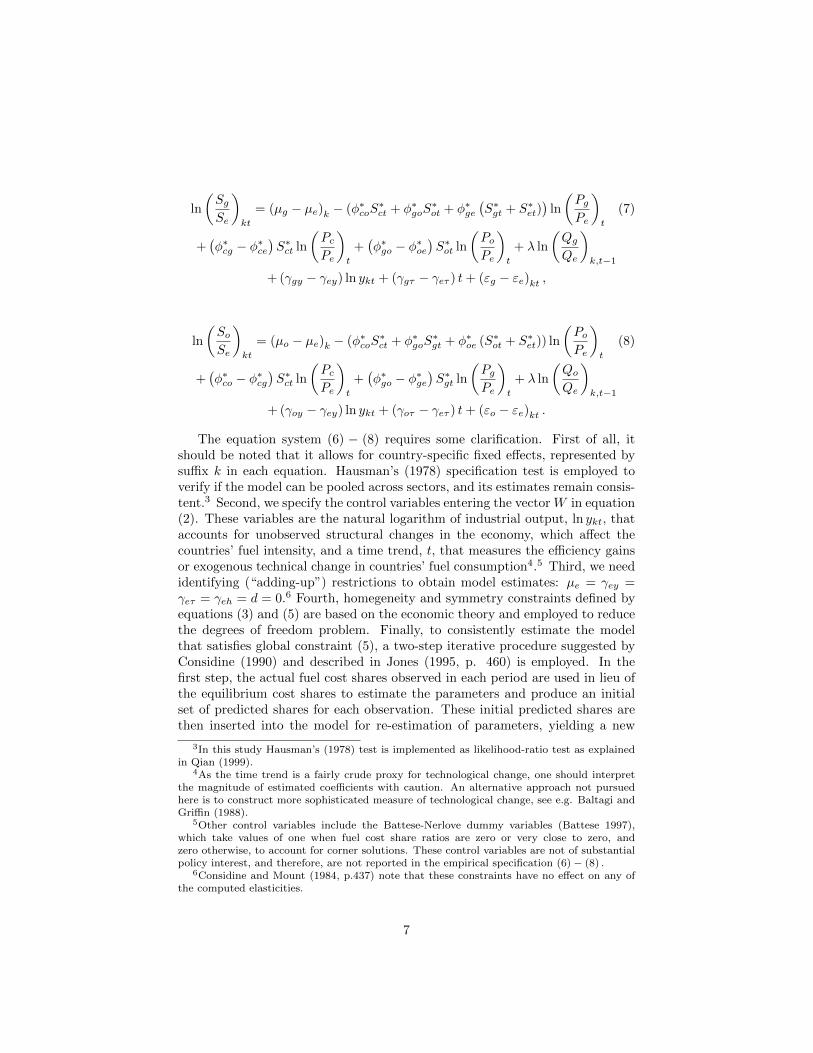
ln
(SgSe
)kt
= (µg − µe)k − (φ∗coS∗ct + φ∗goS
∗ot + φ∗ge
(S∗gt + S∗et)
)ln
(PgPe
)t
(7)
+(φ∗cg − φ∗ce
)S∗ct ln
(PcPe
)t
+(φ∗go − φ∗oe
)S∗ot ln
(PoPe
)t
+ λ ln
(QgQe
)k,t−1
+ (γgy − γey) ln ykt + (γgτ − γeτ ) t+ (εg − εe)kt ,
ln
(SoSe
)kt
= (µo − µe)k − (φ∗coS∗ct + φ∗goS
∗gt + φ∗oe (S∗ot + S∗et)) ln
(PoPe
)t
(8)
+(φ∗co − φ∗cg
)S∗ct ln
(PcPe
)t
+(φ∗go − φ∗ge
)S∗gt ln
(PgPe
)t
+ λ ln
(QoQe
)k,t−1
+ (γoy − γey) ln ykt + (γoτ − γeτ ) t+ (εo − εe)kt .
The equation system (6) − (8) requires some clarification. First of all, itshould be noted that it allows for country-specific fixed effects, represented bysuffix k in each equation. Hausman’s (1978) specification test is employed toverify if the model can be pooled across sectors, and its estimates remain consis-tent.3 Second, we specify the control variables entering the vector W in equation(2). These variables are the natural logarithm of industrial output, ln ykt, thataccounts for unobserved structural changes in the economy, which affect thecountries’ fuel intensity, and a time trend, t, that measures the efficiency gainsor exogenous technical change in countries’ fuel consumption4.5 Third, we needidentifying (“adding-up”) restrictions to obtain model estimates: µe = γey =γeτ = γeh = d = 0.6 Fourth, homegeneity and symmetry constraints defined byequations (3) and (5) are based on the economic theory and employed to reducethe degrees of freedom problem. Finally, to consistently estimate the modelthat satisfies global constraint (5), a two-step iterative procedure suggested byConsidine (1990) and described in Jones (1995, p. 460) is employed. In thefirst step, the actual fuel cost shares observed in each period are used in lieu ofthe equilibrium cost shares to estimate the parameters and produce an initialset of predicted shares for each observation. These initial predicted shares arethen inserted into the model for re-estimation of parameters, yielding a new
3In this study Hausman’s (1978) test is implemented as likelihood-ratio test as explainedin Qian (1999).
4As the time trend is a fairly crude proxy for technological change, one should interpretthe magnitude of estimated coefficients with caution. An alternative approach not pursuedhere is to construct more sophisticated measure of technological change, see e.g. Baltagi andGriffin (1988).
5Other control variables include the Battese-Nerlove dummy variables (Battese 1997),which take values of one when fuel cost share ratios are zero or very close to zero, andzero otherwise, to account for corner solutions. These control variables are not of substantialpolicy interest, and therefore, are not reported in the empirical specification (6) − (8) .
6Considine and Mount (1984, p.437) note that these constraints have no effect on any ofthe computed elasticities.
7
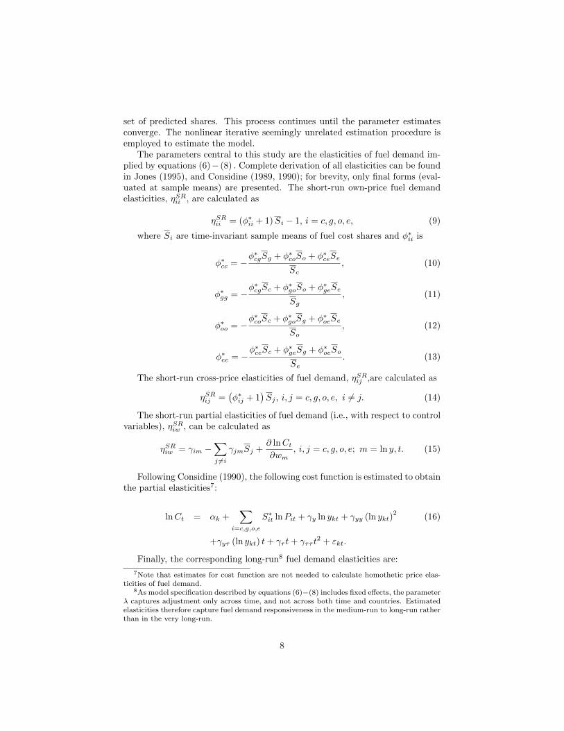
set of predicted shares. This process continues until the parameter estimatesconverge. The nonlinear iterative seemingly unrelated estimation procedure isemployed to estimate the model.
The parameters central to this study are the elasticities of fuel demand im-plied by equations (6)− (8) . Complete derivation of all elasticities can be foundin Jones (1995), and Considine (1989, 1990); for brevity, only final forms (eval-uated at sample means) are presented. The short-run own-price fuel demandelasticities, ηSRii , are calculated as
ηSRii = (φ∗ii + 1)Si − 1, i = c, g, o, e, (9)
where Si are time-invariant sample means of fuel cost shares and φ∗ii is
φ∗cc = −φ∗cgSg + φ∗coSo + φ∗ceSe
Sc, (10)
φ∗gg = −φ∗cgSc + φ∗goSo + φ∗geSe
Sg, (11)
φ∗oo = −φ∗coSc + φ∗goSg + φ∗oeSe
So, (12)
φ∗ee = −φ∗ceSc + φ∗geSg + φ∗oeSo
Se. (13)
The short-run cross-price elasticities of fuel demand, ηSRij ,are calculated as
ηSRij =(φ∗ij + 1
)Sj , i, j = c, g, o, e, i 6= j. (14)
The short-run partial elasticities of fuel demand (i.e., with respect to controlvariables), ηSRiw , can be calculated as
ηSRiw = γim −∑j 6=i
γjmSj +∂ lnCt∂wm
, i, j = c, g, o, e; m = ln y, t. (15)
Following Considine (1990), the following cost function is estimated to obtainthe partial elasticities7:
lnCt = αk +∑
i=c,g,o,e
S∗it lnPit + γy ln ykt + γyy (ln ykt)2
(16)
+γyτ (ln ykt) t+ γτ t+ γττ t2 + εkt.
Finally, the corresponding long-run8 fuel demand elasticities are:
7Note that estimates for cost function are not needed to calculate homothetic price elas-ticities of fuel demand.
8As model specification described by equations (6)−(8) includes fixed effects, the parameterλ captures adjustment only across time, and not across both time and countries. Estimatedelasticities therefore capture fuel demand responsiveness in the medium-run to long-run ratherthan in the very long-run.
8

ηLRij =ηSRij
1− λ, ∀ i, j, (17)
and
ηLRiw =ηSRiw
1− λ, ∀ i, w. (18)
3 Data
The empirical analysis is based on a comprehensive unbalanced panel datasetthat comprises 63 countries over the period 1978 - 2008 (for details, see TableA.1, Appendix I). We focus on the industrial consumption of four fuels - coal,natural gas, petroleum products, and electricity. Following Jones (1995), weexclude the consumption of fuels used for non-energy purposes. Specifically,among coal categories we include steam coal, and exclude coking coal. We com-bine the industrial consumption of natural gas and liquefied petroleum gases(LPG), as those products are close technological substitutes and have similarenergy use (Steinbuks 2012). The petroleum products category comprises con-sumption of light fuel oils, diesel, naphtha, and high-sulphur fuel oils. Finally,we treat electricity as homogenous energy service and do not differentiate acrossthe sources of electricity generation. We obtain country fuel consumption andproduction data from the World Energy Statistics and Balances, published bythe International Energy Agency (IEA).
As fossil fuel production is potentially endogenous to unobserved variablesaffecting fuel demand (e.g., indirect subsidies, government regulations, and capi-tal market imperfections) we use tobit estimates of fuel production instrumentedby countries’ size of natural resource endowment normalized by its 10 year av-erage resource consumption.9 Using natural resource endowment is a naturalchoice for instrumenting fuel production. By Hotelling’s (1931) rule the sizeof natural resource stocks is a critical determinant of fossil fuel extraction de-cision yet it is uncorrelated with unobserved variables mentioned above. Thisinstrumented variable thus reflects not the actual fuel production but rather theextent to which fuel production is feasible (although these measures are closelycorrelated). For information on countries’ natural resource (respectively, coal,natural gas, and oil) endowments we use the BP Statistical Review of WorldEnergy database.10
Table 1 describes the distribution of natural reserves across countries in thedataset in 2008 (for more details, see Table A.2, Appendix I). Most countries in
9We do not instrument for electricity production for two reasons. First, as electricity isdifficult to store and electricity imports are not always reliable, all countries in the sampleproduce electricity. Second, as all countries in the sample have access to renewable electricityresources of some sort (biomass, solar, wind, or hydro), instrumenting for electricity willalways yield positive production.
10Detailed information on the BP Statistical Review of World Energy database canbe found on the following website: http://www.bp.com/en/global/corporate/about-bp/
energy-economics/statistical-review-of-world-energy-2013.html
9
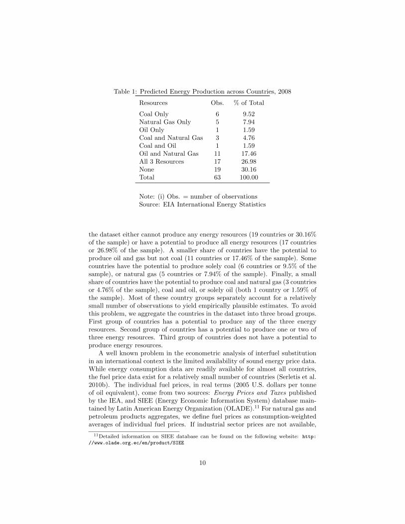
Table 1: Predicted Energy Production across Countries, 2008
Resources Obs. % of Total
Coal Only 6 9.52Natural Gas Only 5 7.94Oil Only 1 1.59Coal and Natural Gas 3 4.76Coal and Oil 1 1.59Oil and Natural Gas 11 17.46All 3 Resources 17 26.98None 19 30.16Total 63 100.00
Note: (i) Obs. = number of observationsSource: EIA International Energy Statistics
the dataset either cannot produce any energy resources (19 countries or 30.16%of the sample) or have a potential to produce all energy resources (17 countriesor 26.98% of the sample). A smaller share of countries have the potential toproduce oil and gas but not coal (11 countries or 17.46% of the sample). Somecountries have the potential to produce solely coal (6 countries or 9.5% of thesample), or natural gas (5 countries or 7.94% of the sample). Finally, a smallshare of countries have the potential to produce coal and natural gas (3 countriesor 4.76% of the sample), coal and oil, or solely oil (both 1 country or 1.59% ofthe sample). Most of these country groups separately account for a relativelysmall number of observations to yield empirically plausible estimates. To avoidthis problem, we aggregate the countries in the dataset into three broad groups.First group of countries has a potential to produce any of the three energyresources. Second group of countries has a potential to produce one or two ofthree energy resources. Third group of countries does not have a potential toproduce energy resources.
A well known problem in the econometric analysis of interfuel substitutionin an international context is the limited availability of sound energy price data.While energy consumption data are readily available for almost all countries,the fuel price data exist for a relatively small number of countries (Serletis et al.2010b). The individual fuel prices, in real terms (2005 U.S. dollars per tonneof oil equivalent), come from two sources: Energy Prices and Taxes publishedby the IEA, and SIEE (Energy Economic Information System) database main-tained by Latin American Energy Organization (OLADE).11 For natural gas andpetroleum products aggregates, we define fuel prices as consumption-weightedaverages of individual fuel prices. If industrial sector prices are not available,
11Detailed information on SIEE database can be found on the following website: http:
//www.olade.org.ec/en/product/SIEE
10

we use different proxies, such as comparable fuel prices in other sectors.We obtain the data on country-level industrial output in real terms (ex-
pressed as the gross value added in manufacturing sector in 2005 U.S. dollars)from the United Nations Statistics Division (http://data.un.org).
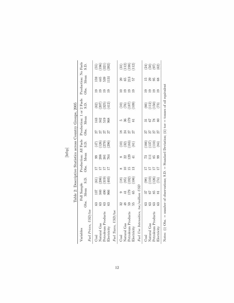
Table 2 shows the descriptive statistics for energy prices, taxes, and con-sumption (relative to output) of fossil fuels and electricity in 2005 across coun-tries grouped by their potential to produce fossil fuels. Countries that have apotential to produce any of the three fossil fuels have considerably lower end-use prices of coal, natural gas, petroleum products, and electricity compared tothe rest of the sample. Countries that cannot produce any fossil fuels have thehighest end-use prices for all energy sources. Energy prices in countries that canproduce one or two fossil fuels are in between two previous groups. The end-useprices of coal, petroleum products, and electricity are about 1.3 to 1.5 timeshigher in countries that cannot produce any fossil fuels. The end-use prices ofnatural gas in these countries are about 2 times higher compared to countriesthat have a potential to produce any of the three fossil fuels, and about 1.3times higher compared to countries that have a potential to produce one or twofossil fuels. The end-use prices of coal, petroleum products, and electricity areof a similar magnitude for countries that have a potential to produce one or twofossil fuels and countries that cannot produce any fossil fuels.
There is a significant heterogeneity in energy taxes across different countrygroups. Taxes on coal and natural gas are considerably (2 to 4 times) lower incountries with the potential to produce all three fossil fuels or at least one fossilfuel, compared to countries that cannot produce fossil fuels. This finding isconsistent with the historical evidence of subsidizing energy production in coaland natural gas rich economies. Taxes on petroleum products across countrygroups exhibit a similar pattern but the difference magnitude (1.2 to 1.65 times)is more subtle. Countries with the potential to produce all three fossil fuels alsohave the lowest tax on electricity, which is 2 times smaller compared to countriesthat have a potential to produce one or two fossil fuels, and 1.4 times smallercompared to countries that cannot produce any fossil fuels.
Table 2 also shows that countries with the potential to produce all three fossilfuels or at least one fossil fuel are more intensive in use of coal, natural gas, andelectricity compared to countries that cannot produce fossil fuels. Countriesthat have a potential to produce any of the three fossil fuels are 4 times moreintensive in their use of coal and natural gas, and 1.5 times more intensive inuse of electricity compared to countries that cannot produce any fossil fuels.Similarly, countries that have a potential to produce one or two of three fossilfuels are 2 times more intensive in their use of coal and natural gas, and 1.2times more intensive in use of electricity compared to countries that cannotproduce any fossil fuels. However, there are no substantial differences in theintensive use of petroleum products across country groups.
11
[htb
p]
Tab
le2:
Des
crip
tive
Sta
tist
ics
acr
oss
Cou
ntr
yG
rou
ps,
2005
Var
iable
sF
ull
Sam
ple
Pro
duct
ion:
All
Fuel
sP
roduct
ion:
1or
2F
uel
sP
roduct
ion:
No
Fuel
sO
bs.
Mea
nS.D
.O
bs.
Mea
nS.D
.O
bs.
Mea
nS.D
.O
bs.
Mea
nS.D
.F
uel
Pri
ces,
US
D/to
e
Coa
l63
137
(61)
17
99(4
7)
27
143
(62)
1915
9(5
5)
Nat
ura
lG
as63
340
(206)
1720
8(1
26)
2734
2(2
07)
19
445
(196)
Pet
role
um
Pro
duct
s63
490
(319
)17
381
(279
)27
519
(325
)19
539
(321)
Ele
ctri
city
6396
6(4
03)
17
764
(296)
27
968
(412
)19
1131
(392
)
Fu
elT
axe
s,U
SD
/to
e
Coa
l32
9(1
8)8
8(1
0)
185
(10)
10
20
(31)
Nat
ura
lG
as48
41(8
5)
1022
(32)
2436
(76)
1965
(112)
Pet
role
um
Pro
duct
s59
179
(192
)15
129
(183
)27
179
(187
)19
213
(198)
Ele
ctri
city
5565
(106)
13
41
(81)
27
81
(109
)19
57
(112
)
Fu
elU
seIn
ten
siti
es,
toe/
mil
lion
US
D
Coa
l63
37(9
8)17
73(1
66)
27
31(6
6)
1915
(24)
Nat
ura
lG
as63
67(1
10)
1711
1(1
37)
2767
(112
)19
29(5
0)P
etro
leum
Pro
duct
s63
85(1
26)
1785
(110
)27
78
(150
)19
95(9
7)E
lect
rici
ty63
81(7
4)17
99
(84)
27
80
(73)
1968
(62)
Not
es:
(i)
Obs.
=num
ber
ofob
serv
atio
ns;
S.D
.=
Sta
ndard
Dev
iati
on;
(ii)
toe
=to
nnes
ofoi
leq
uiv
ale
nt
12
[htb
p]
Tab
le3:
Res
ult
sfo
rM
od
els
of
Fu
elC
onsu
mpti
on
,1978-2
008
Par
amet
erF
ull
Sam
ple
Pro
duct
ion:
All
Fuel
sP
roduct
ion:
1or
2F
uel
sP
roduct
ion:
No
Fuel
sco
eff.
s.e.
coeff
.s.
e.co
eff.
s.e.
coeff
.s.
e.
φ∗ cg
-0.6
2(0
.53)
-0.4
7(1
.92)
-0.2
5(0
.17)
-0.6
9∗∗∗
(0.2
5)
φ∗ co
-0.6
1(0
.66)
-0.5
5(0
.47)
-0.3
6∗∗∗
(0.0
4)-0
.80
(0.6
1)
φ∗ ce
-0.6
3∗∗∗
(0.0
6)-0
.44
(0.3
1)-0
.25∗∗∗
(0.0
2)-0
.83
(34.7
8)φ∗ go
-0.6
1∗∗∗
(0.0
6)-0
.70∗∗∗
(0.0
6)
-0.3
5∗∗∗
(0.1
1)-0
.55∗∗∗
(0.0
5)
φ∗ ge
-0.6
1∗∗∗
(0.0
6)-0
.47∗∗∗
(0.0
4)
-0.7
1∗∗∗
(0.0
7)-0
.79∗∗∗
(0.0
7)
φ∗ oe
-0.9
4∗∗∗
(0.1
0)-0
.94∗∗∗
(0.0
9)
-0.9
9∗∗∗
(0.1
0)-0
.79∗∗∗
(0.0
7)
λ0.3
5∗∗∗
(0.0
4)0.5
7∗∗∗
(0.0
5)
0.2
9∗∗∗
(0.0
3)0.
11∗∗∗
(0.0
1)
γcy
-0.1
2∗∗
(0.0
4)-0
.29∗∗∗
(0.0
3)-0
.07
(0.1
3)0.3
0(0
.47)
γgy
-0.1
2∗∗∗
(0.0
4)-0
.03
(0.6
6)
-0.1
9∗∗∗
(0.0
6)0.0
2∗∗∗
(0.0
02)
γoy
-0.0
8∗∗
(0.0
4)-0
.13∗∗
(0.0
5)-0
.14∗∗
(0.0
6)0.
17∗∗∗
(0.0
2)γcτ
0.00
4∗∗∗
(0.0
004)
0.01
(0.0
7)-0
.01∗∗∗
(0.0
01)
0.000
3∗∗∗
(0.0
001)
γgτ
0.01∗∗∗
(0.0
02)
-0.0
06
(0.0
03)
0.01∗∗∗
(0.0
01)
0.02∗∗∗
(0.0
01)
γoτ
-0.0
2∗∗∗
(0.0
03)
-0.0
1∗∗∗
(0.0
01)
-0.0
3∗∗∗
(0.0
03)
-0.0
4∗∗∗
(0.0
04)
Su
mm
ary
Sta
tist
ics
Obs.
1562
399
684
479
pse
udo-R
2 193
.70
89.8
295.
5597.
91pse
udo-R
2 288
.90
82.5
791.
5093.
02pse
udo-R
2 392
.03
94.7
293.
1086.
88H
ausm
ante
st302
1.2
3(0
.00)
844
.30
(0.0
0)
1627
.64
(0.0
0)
703
.21
(0.0
0)
(χ2
(N),p>χ2)
Not
es:
(i)
Obs.
=num
ber
ofob
serv
atio
ns;
d.f
.=
deg
rees
offr
eedom
.(i
i)E
stim
ates
for
Bat
tese
-Ner
love,
fixed
-eff
ect,
and
stru
ctura
lsh
ift
dum
my
vari
able
sare
not
rep
orte
d,
and
avai
lable
up
onre
ques
t.
13
4 Results
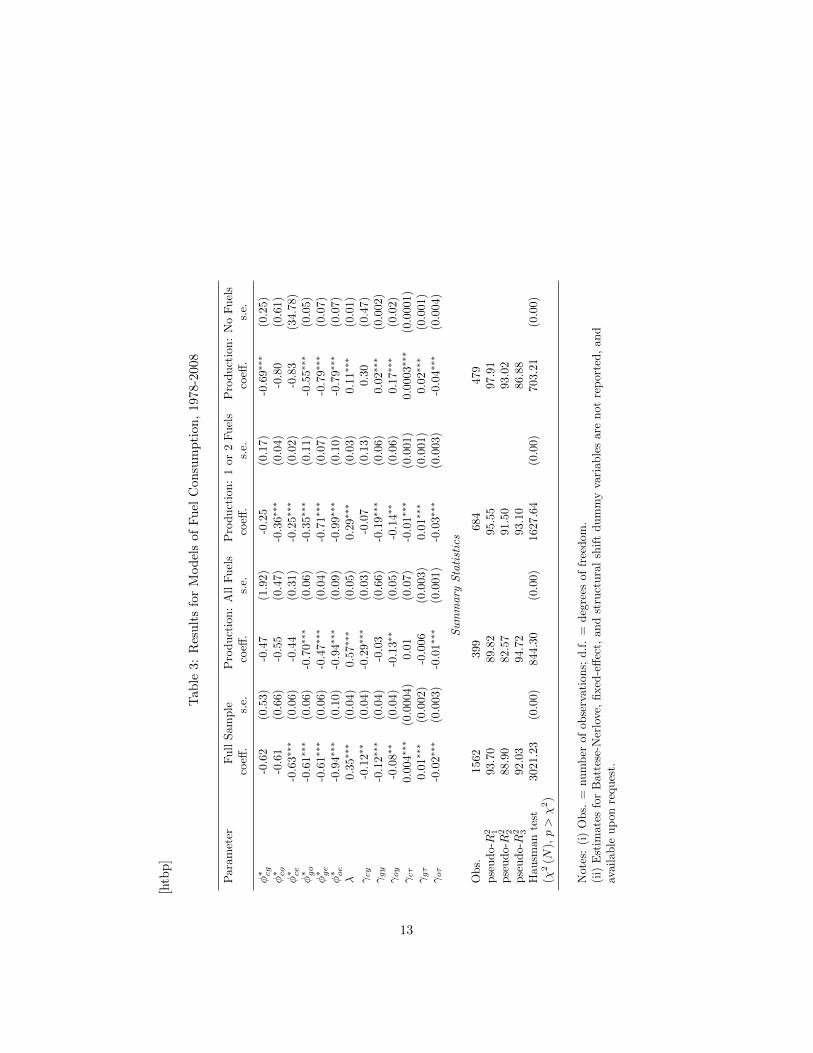
Table 3 presents the parameter estimates and summary statistics for dynamiclinear logit model (equations 6-8) applied to fuel consumption across the entiredataset, and separately to the country groups defined in the previous section. Allmodel specifications have a reasonably good fit, characterized by high pseudo-R squares. The results from Hausman’s (1978) specification test indicate thatthe hypothesis that a pooled model’s estimates are consistent is rejected at a 1percent level of significance for all model specifications. Estimates of structuralparameters φ∗ij vary across country groups, indicating heterogeneity in estimatedelasticities.
Econometric estimates of the adjustment parameter λ reveal that fuel de-mand is responsive in the short-run, with about two-thirds of the long-runresponse taking place in the same year as the price change. The size of theestimated adjustment parameter is the highest for countries that have a po-tential to produce any of the three fossil fuels. For these countries less thana half of the long-run response takes place in the same year as the fuels’ pricechange. The size of the estimated adjustment parameter is considerably smallerfor countries that have a potential to produce one or two fossil fuels. For thesecountries about 70 percent of the long-run response takes place in the sameyear as the fuels’ price change. The size of the estimated adjustment param-eter is the smallest for countries that have no potential to produce any of thethree fossil fuels. For these countries about 90 percent of the long-run responsetakes place in the same year as the fuels’ price change. These results indicatethat more fossil fuel-intensive industries of energy producers have higher capitaladjustment costs, and are consistent with the carbon lock-in hypothesis.
As regards other explanatory variables, the coefficients of the logarithm ofreal gross value added are negative (and, in most cases, statistically significant)across all country groups, except for countries that have no potential to produceany of the three fossil fuels. These results imply that, as output increases,the shares of coal, natural gas, and petroleum products in the industrial fuelmix decline, and the share of electricity increases. For countries that have nopotential to produce any of the three fossil fuels, the coefficients of the logarithmof real gross value added are positive (and statistically significant for naturalgas-to-electricity and petroleum products-to-electricity ratios). These resultsimply that, as output increases, the share of electricity in the industrial fuelmix decreases, and the shares of natural gas and petroleum products increase.
Finally, the estimated coefficients for the time trend are negative and statis-tically significant for the petroleum products-electricity ratio across all groups ofcountries. The estimated coefficients for natural gas-electricity ratio are positiveand statistically significant across all groups of countries, except for the coun-tries that have a potential to produce any of the three fossil fuels. The estimatedcoefficients for coal-electricity ratio are positive and statistically significant forthe full sample, and for countries that have no potential to produce fossil fuels.The estimated coefficients for coal-electricity ratio are positive and not statisti-cally significant for countries that have a potential to produce any of the three
14
fossil fuels. The estimated coefficients for coal-electricity ratio are negative andstatistically significant for countries that have a potential to produce one or twofossil fuels. These results indicate that the direction of the technological changein fuel choice is from petroleum products to electricity and natural gas.
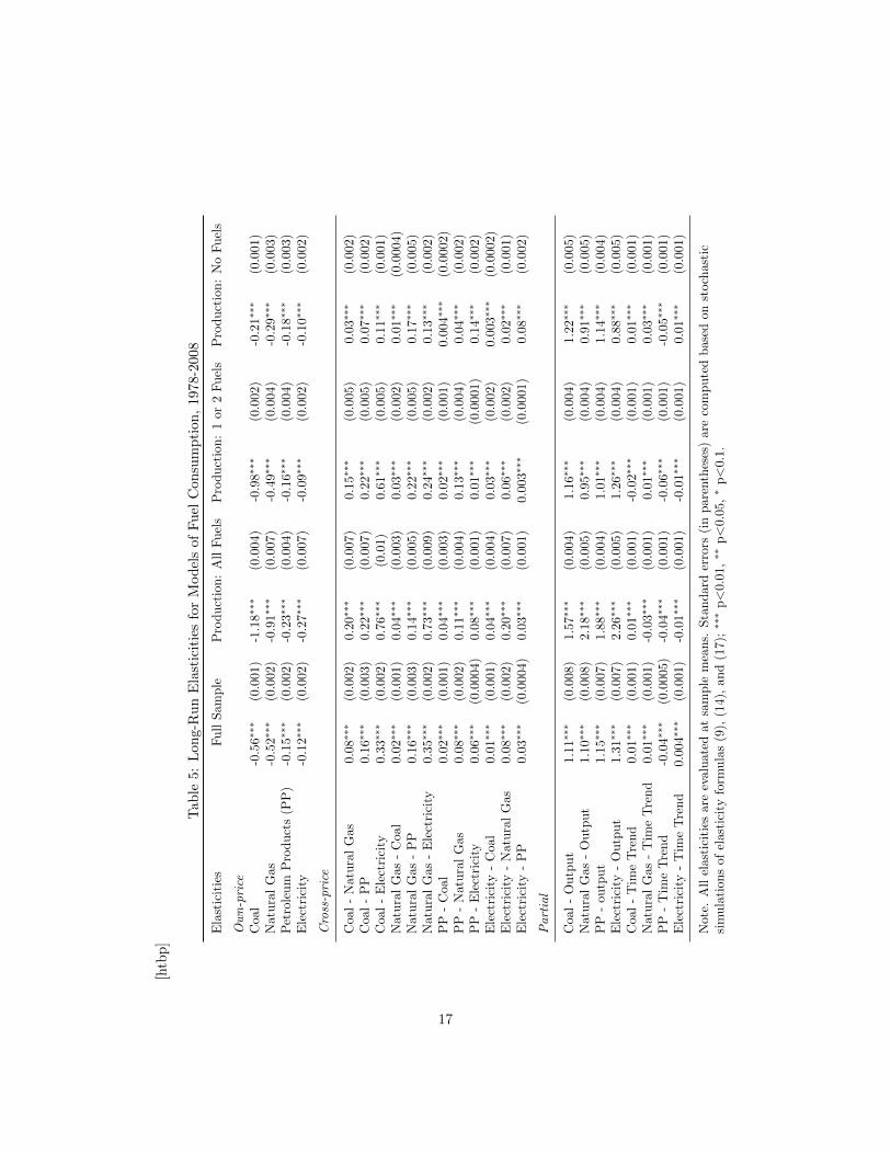
4.1 Elasticities
Tables 4 and 5 show the estimated short-run and long-run elasticities of fueldemand evaluated at the sample means for fuel consumption across the entiredataset, and separately to country groups based on their potential to produceenergy fuels. All of the estimated own-price elasticities are statistically sig-nificant at the 1% level. Estimated elasticities have expected signs and arebroadly comparable to the results from recent studies on international interfuelsubstitution (Serletis et al. 2010b, 2011).12
4.1.1 Own Price Elasticities
The top section of tables 4 and 5 shows the estimated short run and long runown-price elasticities of demand for coal, natural gas, petroleum products, andelectricity. The demand for all fuels is inelastic in both the short-run and thelong-run. Petroleum products and electricity are the most inelastic energy ser-vices, with the estimated short-run own-price elasticities of -0.1 and -0.08, usingthe full dataset. Demand for other fossil fuels is more elastic. Estimated short-run own-price elasticities using full dataset are -0.34 for natural gas and -0.36for coal. In the long run demand for petroleum products and electricity is stillvery unresponsive to fuel prices, with estimated own-price elasticities of -0.15and -0.12, using the full dataset. Demand for coal and natural gas becomesmore responsive to fuel prices, with estimated long-run own-price elasticities of-0.56 and -0.52.
Estimated own-price elasticities of demand for coal vary significantly acrossdifferent country groups. In the short run, own-price elasticities of coal, naturalgas, and electricity demand are all smaller for countries that have no potentialto produce fossil fuels. Own-price elasticities of coal demand in those countriesare about 2.5 times smaller compared to countries that have a potential toproduce all fossil fuels, and about 3.5 times smaller compared to countries thathave a potential to produce one or two fossil fuels. Own-price elasticities ofnatural gas demand in those countries are about 1.5 times smaller compared tocountries that have a potential to produce all fossil fuels. Own-price elasticitiesof electricity demand in those countries are about 1.3 times smaller comparedto countries that have a potential to produce all fossil fuels, but 1.5 times largercompared to countries that have a potential to produce one or two fossil fuels.However, the short run own-price elasticities of petroleum products demand are
12Serletis et al. (2010b) and Serletis et al. (2011) both report Morishima elasticities ofsubstitution, σij . We obtain the estimates of their cross-price elasticities of substitution, ηij ,using ηij = σij + ηjj , where ηjj are the own-price elasticities of substitution.
15

[htb
p]
Tab
le4:
Sh
ort
-Ru
nE
last
icit
ies
for
Mod
els
of
Fu
elC
on
sum
pti
on
,1978-2
008
Ela
stic
itie
sF
ull
Sam
ple
Pro
duct
ion:
All
Fuel
sP
roduct
ion:
1or
2F
uel
sP
roduct
ion:
No
Fuel
s
Ow
n-p
rice
Coa
l-0
.36∗∗∗
(0.0
004
)-0
.51∗∗∗
(0.0
02)
-0.7
0∗∗∗
(0.0
01)
-0.1
9∗∗∗
(0.0
01)
Natu
ral
Gas
-0.3
4∗∗∗
(0.0
01)
-0.3
9∗∗∗
(0.0
03)
-0.3
5∗∗∗
(0.0
03)
-0.2
6∗∗∗
(0.0
02)
Pet
role
um
pro
duct
s(P
P)
-0.1
0∗∗∗
(0.0
01)
-0.1
0∗∗∗
(0.0
02)
-0.1
2∗∗∗
(0.0
03)
-0.1
6∗∗∗
(0.0
03)
Ele
ctri
city
-0.0
8∗∗∗
(0.0
01)
-0.1
2∗∗∗
(0.0
03)
-0.0
6∗∗∗
(0.0
02)
-0.0
9∗∗∗
(0.0
02)
Cro
ss-p
rice
Coa
l-
Natu
ral
Gas
0.05∗∗∗
(0.0
01)
0.0
9∗∗∗
(0.0
03)
0.11∗∗∗
(0.0
04)
0.03∗∗∗
(0.0
01)
Coa
l-
PP
0.10∗∗∗
(0.0
02)
0.1
0∗∗∗
(0.0
03)
0.16∗∗∗
(0.0
04)
0.06∗∗∗
(0.0
02)
Coa
l-
Ele
ctri
city
0.21∗∗∗
(0.0
01)
0.3
3∗∗∗
(0.0
04)
0.44∗∗∗
(0.0
04)
0.10∗∗∗
(0.0
01)
Natu
ral
Gas
-C
oal
0.01∗∗∗
(0.0
004
)0.0
2∗∗∗
(0.0
01)
0.02∗∗∗
(0.0
01)
0.01∗∗∗
(0.0
003
)N
atura
lG
as-
PP
0.10∗∗∗
(0.0
02)
0.0
6∗∗∗
(0.0
02)
0.16∗∗∗
(0.0
04)
0.15∗∗∗
(0.0
04)
Nat
ura
lG
as-
Ele
ctri
city
0.23∗∗∗
(0.0
01)
0.3
1∗∗∗
(0.0
04)
0.17∗∗∗
(0.0
01)
0.12∗∗∗
(0.0
02)
PP
-C
oal
0.0
1∗∗∗
(0.0
004)
0.0
2∗∗∗
(0.0
01)
0.02∗∗∗
(0.0
01)
0.0
03∗∗∗
(0.0
002)
PP
-N
atura
lG
as0.
05∗∗∗
(0.0
01)
0.0
5∗∗∗
(0.0
02)
0.09∗∗∗
(0.0
03)
0.04∗∗∗
(0.0
02)
PP
-E
lect
rici
ty0.
04∗∗∗
(0.0
002)
0.0
3∗∗∗
(0.0
004)
0.0
1∗∗∗
(0.0
001)
0.1
2∗∗∗
(0.0
02)
Ele
ctri
city
-C
oal
0.01∗∗∗
(0.0
004)
0.0
2∗∗∗
(0.0
02)
0.02∗∗∗
(0.0
01)
0.0
03∗∗∗
(0.0
002)
Ele
ctri
city
-N
atura
lG
as0.
05∗∗∗
(0.0
01)
0.0
9∗∗∗
(0.0
03)
0.04∗∗∗
(0.0
01)
0.02∗∗∗
(0.0
01)
Ele
ctri
city
-P
P0.
02∗∗∗
(0.0
003)
0.0
1∗∗∗
(0.0
004)
0.0
02∗∗∗
(0.0
001)
0.0
7∗∗∗
(0.0
02)
Part
ial
Coa
l-
Outp
ut
0.72∗∗∗
(0.0
05)
0.6
8∗∗∗
(0.0
02)
0.83∗∗∗
(0.0
03)
1.08∗∗∗
(0.0
05)
Natu
ral
Gas
-O
utp
ut
0.71∗∗∗
(0.0
05)
0.9
4∗∗∗
(0.0
02)
0.67∗∗∗
(0.0
03)
0.80∗∗∗
(0.0
05)
PP
-O
utp
ut
0.74∗∗∗
(0.0
05)
0.8
1∗∗∗
(0.0
02)
0.72∗∗∗
(0.0
03)
1.01∗∗∗
(0.0
04)
Ele
ctri
city
-O
utp
ut
0.85∗∗∗
(0.0
05)
0.9
8∗∗∗
(0.0
02)
0.90∗∗∗
(0.0
03)
0.78∗∗∗
(0.0
05)
Coa
l-
Tim
eT
rend
0.01∗∗∗
(0.0
003
)0.
004∗∗∗
(0.0
01)
-0.0
1∗∗∗
(0.0
01)
0.01∗∗∗
(0.0
01)
Natu
ral
Gas
-T
ime
Tre
nd
0.01∗∗∗
(0.0
003
)-0
.01∗∗∗
(0.0
01)
0.01∗∗∗
(0.0
01)
0.03∗∗∗
(0.0
01)
PP
-T
ime
Tre
nd
-0.0
3∗∗∗
(0.0
003
)-0
.02∗∗∗
(0.0
01)
-0.0
4∗∗∗
(0.0
01)
-0.0
5∗∗∗
(0.0
01)
Ele
ctri
city
-T
ime
Tre
nd
0.00
2∗∗∗
(0.0
003
)-0
.004∗∗∗
(0.0
01)
-0.0
1∗∗∗
(0.0
01)
0.01∗∗∗
(0.0
01)
Not
e.A
llel
asti
citi
esar
eev
aluat
edat
sam
ple
mea
ns.
Sta
ndard
erro
rs(i
npar
enth
eses
)ar
eco
mpute
dbase
don
stoch
asti
csi
mula
tion
sof
elas
tici
tyfo
rmula
s(9
),(1
4),
and
(17);∗∗∗
p<
0.0
1,∗∗
p<
0.0
5,∗
p<
0.1.
16
[htb
p]
Tab
le5:
Lon
g-R
un
Ela
stic
itie
sfo
rM
od
els
of
Fu
elC
on
sum
pti
on
,1978-2
008
Ela
stic
itie
sF
ull
Sam
ple
Pro
duct
ion:
All
Fuel
sP
roduct
ion:
1or
2F
uel
sP
roduct
ion:
No
Fuel
s
Ow
n-p
rice
Coa
l-0
.56∗∗∗
(0.0
01)
-1.1
8∗∗∗
(0.0
04)
-0.9
8∗∗∗
(0.0
02)
-0.2
1∗∗∗
(0.0
01)
Nat
ura
lG
as-0
.52∗∗∗
(0.0
02)
-0.9
1∗∗∗
(0.0
07)
-0.4
9∗∗∗
(0.0
04)
-0.2
9∗∗∗
(0.0
03)
Pet
role
um
Pro
duct
s(P
P)
-0.1
5∗∗∗
(0.0
02)
-0.2
3∗∗∗
(0.0
04)
-0.1
6∗∗∗
(0.0
04)
-0.1
8∗∗∗
(0.0
03)
Ele
ctri
city
-0.1
2∗∗∗
(0.0
02)
-0.2
7∗∗∗
(0.0
07)
-0.0
9∗∗∗
(0.0
02)
-0.1
0∗∗∗
(0.0
02)
Cro
ss-p
rice
Coa
l-
Natu
ral
Gas
0.08∗∗∗
(0.0
02)
0.20∗∗∗
(0.0
07)
0.1
5∗∗∗
(0.0
05)
0.03∗∗∗
(0.0
02)
Coa
l-
PP
0.16∗∗∗
(0.0
03)
0.22∗∗∗
(0.0
07)
0.2
2∗∗∗
(0.0
05)
0.07∗∗∗
(0.0
02)
Coa
l-
Ele
ctri
city
0.33∗∗∗
(0.0
02)
0.76∗∗∗
(0.0
1)0.
61∗∗∗
(0.0
05)
0.11∗∗∗
(0.0
01)
Natu
ral
Gas
-C
oal
0.02∗∗∗
(0.0
01)
0.04∗∗∗
(0.0
03)
0.0
3∗∗∗
(0.0
02)
0.01∗∗∗
(0.0
004
)N
atura
lG
as-
PP
0.16∗∗∗
(0.0
03)
0.14∗∗∗
(0.0
05)
0.2
2∗∗∗
(0.0
05)
0.17∗∗∗
(0.0
05)
Nat
ura
lG
as-
Ele
ctri
city
0.35∗∗∗
(0.0
02)
0.73∗∗∗
(0.0
09)
0.2
4∗∗∗
(0.0
02)
0.13∗∗∗
(0.0
02)
PP
-C
oal
0.0
2∗∗∗
(0.0
01)
0.04∗∗∗
(0.0
03)
0.0
2∗∗∗
(0.0
01)
0.0
04∗∗∗
(0.0
002)
PP
-N
atura
lG
as0.
08∗∗∗
(0.0
02)
0.11∗∗∗
(0.0
04)
0.1
3∗∗∗
(0.0
04)
0.04∗∗∗
(0.0
02)
PP
-E
lect
rici
ty0.
06∗∗∗
(0.0
004)
0.0
8∗∗∗
(0.0
01)
0.0
1∗∗∗
(0.0
001)
0.1
4∗∗∗
(0.0
02)
Ele
ctri
city
-C
oal
0.01∗∗∗
(0.0
01)
0.04∗∗∗
(0.0
04)
0.0
3∗∗∗
(0.0
02)
0.0
03∗∗∗
(0.0
002)
Ele
ctri
city
-N
atura
lG
as0.
08∗∗∗
(0.0
02)
0.20∗∗∗
(0.0
07)
0.06∗∗∗
(0.0
02)
0.02∗∗∗
(0.0
01)
Ele
ctri
city
-P
P0.
03∗∗∗
(0.0
004)
0.0
3∗∗∗
(0.0
01)
0.0
03∗∗∗
(0.0
001)
0.08∗∗∗
(0.0
02)
Part
ial
Coa
l-
Outp
ut
1.11∗∗∗
(0.0
08)
1.57∗∗∗
(0.0
04)
1.1
6∗∗∗
(0.0
04)
1.22∗∗∗
(0.0
05)
Natu
ral
Gas
-O
utp
ut
1.10∗∗∗
(0.0
08)
2.18∗∗∗
(0.0
05)
0.9
5∗∗∗
(0.0
04)
0.91∗∗∗
(0.0
05)
PP
-ou
tput
1.15∗∗∗
(0.0
07)
1.88∗∗∗
(0.0
04)
1.0
1∗∗∗
(0.0
04)
1.14∗∗∗
(0.0
04)
Ele
ctri
city
-O
utp
ut
1.31∗∗∗
(0.0
07)
2.26∗∗∗
(0.0
05)
1.2
6∗∗∗
(0.0
04)
0.88∗∗∗
(0.0
05)
Coa
l-
Tim
eT
rend
0.01∗∗∗
(0.0
01)
0.01∗∗∗
(0.0
01)
-0.0
2∗∗∗
(0.0
01)
0.01∗∗∗
(0.0
01)
Nat
ura
lG
as-
Tim
eT
rend
0.01∗∗∗
(0.0
01)
-0.0
3∗∗∗
(0.0
01)
0.01∗∗∗
(0.0
01)
0.03∗∗∗
(0.0
01)
PP
-T
ime
Tre
nd
-0.0
4∗∗∗
(0.0
005
)-0
.04∗∗∗
(0.0
01)
-0.0
6∗∗∗
(0.0
01)
-0.0
5∗∗∗
(0.0
01)
Ele
ctri
city
-T
ime
Tre
nd
0.00
4∗∗∗
(0.0
01)
-0.0
1∗∗∗
(0.0
01)
-0.0
1∗∗∗
(0.0
01)
0.01∗∗∗
(0.0
01)
Not
e.A
llel
asti
citi
esar
eev
aluat
edat
sam
ple
mea
ns.
Sta
ndard
erro
rs(i
npar
enth
eses
)ar
eco
mpute
dbase
don
stoch
asti
csi
mula
tion
sof
elas
tici
tyfo
rmula
s(9
),(1
4),
and
(17);∗∗∗
p<
0.0
1,∗∗
p<
0.0
5,∗
p<
0.1.
17
1.3 to 1.6 times larger for countries that have no potential to produce fossil fuelsrelative to energy-producing countries.
In the long-run, own-price elasticities of demand for all energy sources arelarger for countries that have potential to produce any of fossil fuels. Own-priceelasticities of coal demand in those countries are about 6 times larger comparedto countries that have no potential to produce any of energy fuels, and about 1.2times larger compared to countries that have a potential to produce one or twofossil fuels. Own-price elasticities of natural gas demand in those countries areabout 3 times larger compared to countries that have no potential to produceall fossil fuels, and about 1.8 times larger compared to countries that have apotential to produce one or two fossil fuels. Own-price elasticities of petroleumproducts demand in those countries are about 1.3 to 1.4 times larger comparedto countries that have a potential to produce one or two of fossil fuels or cannotproduce any fossil fuels. Own-price elasticities of electricity demand in thosecountries are about 3 times larger compared to countries that have a potentialto produce one or two of fossil fuels or cannot produce any energy fuels.
4.1.2 Cross Price Elasticities
The middle section of tables 4 and 5 shows the estimated short run and long runcross-price elasticities of fuel demand with respect coal, natural gas, petroleum,and electricity prices. Estimated cross-price elasticities are all positive in bothshort- and the long run, indicating that all four fuels are substitutes. Thoseelasticities are, however, small in their absolute magnitude (less or equal to 0.23in the short-run, using full dataset), indicating limited possibilities for inter-fuelsubstitution. The largest scope for interfuel substitution is for coal and naturalgas with respect to electricity prices (0.21 and 0.23 in the short-run using fulldataset) and petroleum products prices (0.1 in the short-run using full dataset).Both petroleum products and electricity appear to be very poor substitutes toother fuels with estimated short-run elasticities less than 0.05 using full dataset.
As regards variation across country groups based on natural resources, es-timates of both short and long run cross-price elasticities do vary significantlyacross different country groups. Specifically, estimated cross-price elasticitiesof coal with respect to other fuels’ prices, and cross-price elasticities of otherfuels with respect to coal’s prices are all considerably higher for countries withthe potential to produce all fossil fuels or at least one fossil fuel. The largestestimated short run cross-price elasticity is of coal with respect to electricityprices for countries with the potential to produce at least one fossil fuel (0.44),which is more than 4 times higher than for countries with no potential to pro-duce any fossil fuels. Similarly, estimated short run cross-price elasticities ofnatural gas with respect to electricity prices, and of electricity and petroleumproducts with respect to natural gas prices are higher for countries with thepotential to produce all fossil fuels or at least one fossil fuel. These differencesbecome even more pronounced in the long run. This is because (as shown in thesection above) the countries with the potential to produce fossil fuels accountfor smaller share of the long-run response in the year of the fuels’ price change.
18
On the contrary, estimated cross-price elasticities of petroleum products withrespect to electricity prices, and of electricity with respect to petroleum pricesare higher for countries with the potential to produce all fossil fuels or at leastone fossil fuel. Finally, estimated short run cross-price elasticity of natural gaswith respect to petroleum prices, is smaller for countries with the potential toproduce all fossil fuels than in other countries. This difference becomes smallerin the long run.
4.1.3 Partial Elasticities
The bottom section of tables 4 and 5 shows the estimated partial elasticities offuel demand with respect to changes in manufacturing output and time trend.Estimated average elasticities of fuel demand with respect to output are allpositive and less than one, indicating that “as output increases there will besubstitution away from energy” (Pindyck 1979, p. 176). In the long-run, outputelasticities of fuel demand are all above one, which implies that an increasein output results in more than proportional increase in energy consumption.Estimated short run elasticities of coal and petroleum products demand withrespect to output are largest for countries with no potential to produce fossilfuels. Estimated short run elasticities of natural gas and electricity demandwith respect to output are largest for countries with the potential to produceall fossil fuels. Estimated long run elasticities of all four fuels with respect tooutput are largest for countries with the potential to produce all fossil fuels.
Estimated average elasticities of fuel demand with respect to time trendare positive for coal, natural gas and electricity, and negative for petroleumproducts. This result implies that the technological change results in greaterconsumption of coal, natural gas and electricity, and smaller consumption ofpetroleum products. However, the estimated elasticities of fuel demand withrespect to time trend are negative for natural gas, petroleum products, andelectricity for countries with the potential to produce all fossil fuels. Similarly,the estimated elasticities of fuel demand with respect to time trend are negativefor coal, petroleum products, and electricity for countries with the potential toproduce at least one fossil fuel. These results indicate that technological changeresults in smaller fuel consumption in energy producing economies.
5 Counterfactual Analysis using GTAP-E Model
This section applies econometric estimates from dynamic linear logit model toevaluate the effects of energy and climate policies in energy producing and non-producing countries. Because dynamic linear logit model is a partial equilibriummodel, and cannot account for all market mediated responses, for our analysiswe employ computable general equilibrium (CGE) model GTAP-E (Burniauxand Truong 2002). GTAP-E is a special extension of a widely used multi-sectormulti-country GTAP model (Hertel 1997). In GTAP model, consumers are rep-resented by a utility-maximizing private household, whose preferences are de-
19
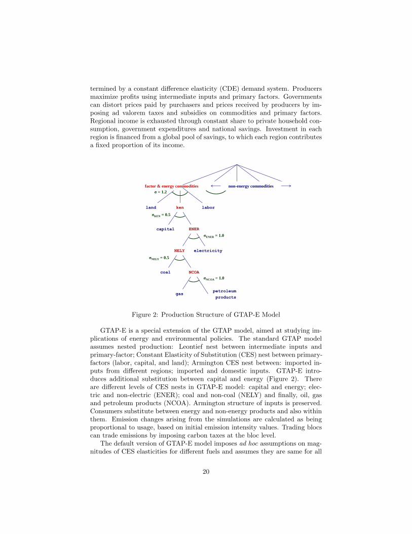
termined by a constant difference elasticity (CDE) demand system. Producersmaximize profits using intermediate inputs and primary factors. Governmentscan distort prices paid by purchasers and prices received by producers by im-posing ad valorem taxes and subsidies on commodities and primary factors.Regional income is exhausted through constant share to private household con-sumption, government expenditures and national savings. Investment in eachregion is financed from a global pool of savings, to which each region contributesa fixed proportion of its income.
o σ = 0.0
land
capital
factor & energy commodities
labor ken
ENER
non-energy commodities
σ = 1.2
σKEN = 0.5
coal
gas
NELY electricity
petroleum
products
NCOA
σNELY = 0.5
σNCOA = 1.0
σENER = 1.0
Figure 2: Production Structure of GTAP-E Model
GTAP-E is a special extension of the GTAP model, aimed at studying im-plications of energy and environmental policies. The standard GTAP modelassumes nested production: Leontief nest between intermediate inputs andprimary-factor; Constant Elasticity of Substitution (CES) nest between primary-factors (labor, capital, and land); Armington CES nest between: imported in-puts from different regions; imported and domestic inputs. GTAP-E intro-duces additional substitution between capital and energy (Figure 2). Thereare different levels of CES nests in GTAP-E model: capital and energy; elec-tric and non-electric (ENER); coal and non-coal (NELY) and finally, oil, gasand petroleum products (NCOA). Armington structure of inputs is preserved.Consumers substitute between energy and non-energy products and also withinthem. Emission changes arising from the simulations are calculated as beingproportional to usage, based on initial emission intensity values. Trading blocscan trade emissions by imposing carbon taxes at the bloc level.
The default version of GTAP-E model imposes ad hoc assumptions on mag-nitudes of CES elasticities for different fuels and assumes they are same for all
20

countries. We replace the default energy substitution elasticities with the elas-ticities derived from our econometric results. To use the results from dynamiclinear logit model in CGE framework we have to convert calculated cross-priceelasticities to CES elasticities of substitution. The relationship between short-run cross-price elasticities, ηSRij , and CES elasticities of substitution, σij , aregiven by
σij =ηSRij
Si. (19)
Table 6 shows calculated CES elasticities across different country groups. Byaveraging across the σ’s, we calculate the CES elasticities needed for the GTAP-E model: all the elasticities between coal and non-coal fuels for the NELY nest;those between electricity and non-electric fuels for the ENER nest. For theNCOA nest, the only elasticity needed is that between oil and gas.
Table 6: CES Elasticities for revised GTAP-E model
Elasticities Full Production: Production: Production:Sample All Fuels 1 or 2 Fuels No Fuels
σce 0.37 0.56 0.75 0.17σge 0.39 0.53 0.29 0.21σoe 0.06 0.06 0.01 0.21σENER 0.28 0.38 0.35 0.20
σcg 0.38 0.53 0.75 0.31σco 0.37 0.45 0.64 0.20σNELY 0.38 0.49 0.69 0.25
σNCOA 0.39 0.30 0.65 0.45
Notes: (i) σNCOA = σgo; (ii) σNELY = 12 (σco + σcg);
(iii) σENER = 13 (σce + σge + σoe).
Using these calculations, we conduct counterfactual simulations to test theimplications of differences in elasticities of fuel substitution across different coun-try groups. We employ revised GTAP-E version (McDougall and Golub 2007),which is based on GTAP 7.1 Data Base (Narayanan and Walmsley 2008) witha base year of 2004. We aggregate the 112 regions in the data base into threegroups: those with no potential to produce fossil fuels, those with potential toproduce all fossil fuels and those with the potential to produce one or two fossilfuels, based on our estimation results.13 We follow Burniaux and Truong (2002)in the sectoral aggregation from 57 GTAP sectors to 8 sectors: agriculture, coal,
13For countries where estimation results were not available we used actual instead of pre-dicted energy production.
21
oil, natural gas, oil products, electricity, energy intensive industries (en int ind)and other industries and services (oth ind ser).
We use two different sets of fuel substitution elasticities: one that employsthe elasticities estimated using full sample (as baseline); another that employsregion-specific elasticities as shown in table 6. With each of these sets of elas-ticities we conduct two independent policy experiments. In first experimentimpose a uniform carbon tax of US$ 30 per ton of CO2 across all countries. Inthe second experiment, we increase production and consumption taxes on theusage of oil (and oil products) to the extent that all existing oil subsidies areeliminated. Our estimate of fossil fuel subsidies are based on the report by theIEA et al. (2010), which quotes the total subsidy bill as being US$ 557 billion for37 non-OECD economies in 2008. Given that many other countries includingthe OECD economies are left out of that report, this estimate represents thelower bound of fossil fuel subsidies. Even this turns out to be over 25% of totalexpenditure on oil and oil products by firms and private households in GTAPData Base. Thus we assume an increase of tax rates on firm and householdconsumption of all these products by 25 percentage points, as the equivalent forthe removal of fossil fuel subsidies for policy experiment 2.
The mechanisms with which carbon tax and elimination of fuel subsidiesact in GTAP-E model are different, though they both act as wedge betweendifferent prices. Carbon taxes are imposed in specific terms (e.g., US$ perunit of carbon) on all commodities and agents, weighted by the correspondingemission intensity. For example, a carbon tax of 10 US$ per ton of carbonwill result in 10 percent increase in commodity prices if the emission intensityassociated with the private household consumption of that commodity is 0.01ton of carbon per US$. All other taxes and subsidies in the GTAP-E modelare represented as ad valorem percent changes. In our example, the power ofsubsidies14 should be reduced by 10% of its initial value to achieve a similareffect of 10 percent increase agents’ prices. Thus, for changes in subsidies toaffect the agents’ prices, emissions intensities are irrelevant.
Table 7 shows the differences between the results of changes in sectoral out-put from the counterfactual and baseline simulations, for each of the 2 ex-periments, in millions of US$ (for details of these simulations, see Table A.3,Appendix I). These results demonstrate that the effect of energy and climatepolicies depends critically on the extent to which countries can substitute be-tween different fuels.
First, let us consider the implications of fuel substitution on the carbon taxpolicy. As explained above the effect of carbon tax on energy prices dependscritically on emission intensities of fossil fuels. These intensities are the highestfor coal (∼ 3.7 tCO2 / toe), followed by oil and oil products (∼ 2.9 - 3.1 tCO2
/ toe), and natural gas (∼ 2.2 tCO2 / toe).15 We would thus expect thata carbon tax will result in a substitution from coal to less carbon intensive
14Power of tax or subsidy is defined as one plus rate of tax or subsidy. For example, if therate of tax is 0.1 or 10%, power of tax is 1.1.
15The emission intensity of electricity is difficult to determine as it is idiosyncratic to gen-eration fuel mix in each country.
22

Table 7: Output change differences between the counterfactual and baselinesimulations using GTAP-E model (in USD million)
Industry Carbon Tax Oil Subsidies Removal
Production: Production: Production: Production: Production: Production:All Fuels 1 or 2 Fuels No Fuels All Fuels 1 or 2 Fuels No Fuels
Agriculture 14 -37 14 -15 16 1Coal -2120 -263 20 413 41 5Oil 470 403 37 -406 -286 -21Gas 1020 83 23 -596 -5 -10Oil Products 464 1171 -58 -485 -557 23Electricity 464 86 -61 2059 537 20En int ind 414 -564 11 -350 341 22Oth ind ser 132 -594 -194 -464 258 83Total 857 285 -208 156 346 122
Note: Baseline simulations employ fuel substitution elasticities estimated using full sample andreported in column 2 of Table 6. Counterfactual simulations employ fuel substition elasticitiesestimated using region-specific subsamples reported in columns 3, 4, and 5 of Table 6.
fuels. As shown in table 6 countries with potential to produce all fossil fuelsand countries with potential to produce one or two fossil fuels have higher thanaverage elasticities of substitution of coal for oil, natural gas, and electricity.Table 7 shows that production of coal declines and production of natural gasand electricity increases by a greater amount in these countries. Comparedto baseline scenario the consumption of coal declines by additional 2120 $USmillion in countries with potential to produce all fossil fuels, and by additional263 $US million in countries with potential to produce one or two fossil fuels.The production of natural gas and electricity increase by additional 1020 and464 $US million in countries with potential to produce all fossil fuels, and byadditional 83 and 86 $US million in countries with potential to produce one ortwo fossil fuels.
Next, let us consider the implications of fuel substitution on the policy ofphasing out oil subsidies. Reduction in oil subsidies increases the relative priceof oil and oil products. We would thus expect that the policy of phasing out oilsubsidies will result in a substitution from oil to coal, electricity, and natural gas.As shown in table 6 countries with potential to produce all fossil fuels have higherthan average elasticities of substitution of oil for coal and electricity, and lowerthan average elasticities of substitution of oil for natural gas. Table 7 shows thatproduction of oil, oil products and natural gas declines and production of coaland electricity increases by a greater amount in these countries. Compared tobaseline scenario consumption of oil, oil products, and natural gas declines byadditional 406, 485, and 596 $US million in countries with potential to produceall fossil fuels. Production of coal and electricity increase by additional 413 and2059 $US million in countries with potential to produce all fossil fuels. Table 6demonstrates that countries with potential to produce one or two energy fuelshave higher than average elasticities of substitution of oil for coal, natural gasand electricity. Table 7 shows that production of oil and oil products declines
23
and production of coal and electricity increases by a greater amount in thesecountries. Compared to baseline scenario consumption of oil and oil productsdeclines by additional 286, and 557 $US million in countries with potential toproduce one or two fossil fuels. Production of coal and electricity increase byadditional 41 and and 537 $US million in countries with potential to produceone or two fossil fuels.
6 Conclusions
This study extends the literature on interfuel substitution by investigating therole of transactions costs and technological adjustment, focusing specifically ondifferences across countries with different potential for fossil fuel production. Weestimate an econometric model of interfuel substitution using a large unbalancedpanel dataset of 63 countries, and calculate elasticities of energy demand forfossil fuel producing and non-producing economies.
We find that countries with the potential to produce coal, natural gas, or oilhave higher elasticities of fuel substitution. In many cases short run elasticitiesof fuel substitution for countries with a potential to produce fossil fuels arehigher than long run elasticities for countries with no potential to produce fossilfuels. We also find that countries with a potential to produce all fossil fuelsor at least one fossil fuel have a considerably longer adjustment of fuel-usingcapital stocks. For these, more energy-intensive, countries, the share of sameyear response to fuels’ price change was less than fifty percent as opposed toninety percent in countries with no potential to produce any fossil fuels. Asa result, countries with a potential to produce any of the available fossil fuelshave considerably higher difference between short and long run elasticities offuel substitution.
We then use calculated elasticities to evaluate the effects of a carbon taxand reduction in oil subsidies using GTAP-E computable general equilibriummodelling framework. Our simulations show that, compared to the baselinecase of uniform elasticities of fuel substitution, carbon tax results in a greaterdecline in coal consumption in countries with a potential to produce fossil fuels,as these countries have larger elasticities of substitution of coal for natural gasand electricity. Compared to the baseline case, reduction in oil subsidies lowersproduction of oil, oil products and natural gas and raises production of coaland electricity by a greater amount in countries with a potential produce allfossil fuels. And production of oil and oil products declines and production ofcoal, natural gas, and electricity increases by a greater amount in countries withpotential produce one or two fossil fuels.
These results are important because they imply lower economic cost forpolicies aimed at climate abatement and more efficient utilization of energyresources.
24
References
Armington, P.: 1969, A Theory of Demand for Products Distinguished by Placeof Production, IMF Staff papers 17, 159–176.
Balistreri, E., Al-Qahtani, A. and Dahl, C.: 2010, Oil and Petroleum ProductArmington Elasticities: A New-Geography-of-Trade Approach to Estimation,The Energy Journal 31(3).
Baltagi, B. and Griffin, J.: 1988, A General Index of Technical Change, TheJournal of Political Economy 96(1), 20–41.
Battese, G.: 1997, A Note on the Estimation of Cobb-Douglas Production Func-tions When Some Explanatory Variables Have Zero Values, Journal of Agri-cultural Economics 48(1-3), 250–252.
Berndt, E., Morrison, C. and Watkins, G.: 1981, Dynamic Models of Energy De-mand: An Assessment and Comparison, in Measuring and Modeling NaturalResource Substitution (ed. E. Berndt and B. Field), MIT Press.
Bosetti, V., Carraro, C., Galeotti, M., Massetti, E. and Tavoni, M.: 2006,A World Induced Technical Change Hybrid Model, The Energy Journal27(S2), 13–38.
Brannlund, R. and Lundgren, T.: 2004, A Dynamic Analysis of Interfuel Sub-stitution for Swedish Heating Plants, Energy Economics 26(6), 961–976.
Burniaux, J.-M. and Chateau, J.: 2008, An Overview of the OECD ENV-Linkages Model, OECD Economics Department Working Paper 653, OECDPublishing.
Burniaux, J.-M. and Chateau, J.: 2011, Mitigation Potential of Removing Fos-sil Fuel Subsidies: A General Equilibrium Assessment, OECD EconomicsDepartment Working Paper 853, OECD Publishing.
Burniaux, J. and Truong, T.: 2002, GTAP-E: An Energy-Environmental Ver-sion of the GTAP Model, GTAP Technical Paper 16, Center for Global TradeAnalysis, Purdue University.
Chavas, J. and Segerson, K.: 1986, Singularity and Autoregressive Disturbancesin Linear Logit Models, Journal of Business & Economic Statistics 4(2), 161–169.
Considine, T.: 1989, Separability, Functional Form and Regulatory Policy inModels of Interfuel Substitution, Energy Economics 11(2), 82–94.
Considine, T.: 1990, Symmetry constraints and variable returns to scale in logitmodels, Journal of Business & Economic Statistics 8(3), 347–353.
25
Considine, T. and Mount, T.: 1984, The Use of Linear Logit Models for DynamicInput Demand Systems, The Review of Economics and Statistics 66(3), 434–443.
Hausman, J.: 1978, Specification Tests in Econometrics, Econometrica46(6), 1251–1272.
Hertel, T. W.: 1997, Global Trade Analysis: Modeling and Applications, Cam-bridge University Press.
Hotelling, H.: 1931, The Economics of Exhaustible Resources, The Journal ofPolitical Economy 39(2), 137–175.
IEA, OPEC, OECD and World Bank: 2010, Analysis of the Scope of EnergySubsidies and Suggestions for the G-20 Initiative, Joint report, prepared forsubmission to the G-20 meeting of the Finance Ministers and Central BankGovernors, Busan (Korea), 5 June and 26 May.
IPCC: 2007, Climate Change 2007: Synthesis Report, Contribution of workinggroups i, ii and iii to the fourth assessment report of the intergovernmen-tal panel on climate change, Intergovernmental Panel on Climate Change:Geneva, Switzerland.
Jacoby, H. D. and Wing, I. S.: 1999, Adjustment Time, Capital Malleabilityand Policy Cost, Energy Journal 20(S), 73–92.
Jones, C.: 1995, A Dynamic Analysis of Interfuel Substitution in US IndustrialEnergy Demand, Journal of Business & Economic Statistics 13(4), 459–465.
Jones, C.: 1996, A Pooled Dynamic Analysis of Interfuel Substitution in Indus-trial Energy Demand by the G-7 Countries, Applied Economics 28(7), 815–821.
Kim, S. H., Edmonds, J., Lurz, J., Smith, S. J. and Wise, M.: 2006, TheObjECTS Framework for Integrated Assessment: Hybrid Modeling of Trans-portation, The Energy Journal 27(S2), 63–92.
Kosmo, M.: 1987, Money to Burn. The High Costs of Energy Subsidies, Workingpaper, World Resources Institute, Washington, DC.
Manne, A. and Richels, R.: 2005, MERGE: An Integrated Assessment Modelfor Global Climate Change, Energy and Environment pp. 175–189.
McDougall, R. and Golub, A.: 2007, GTAP-E: A Revised Energy-Environmental Version of the GTAP Model, GTAP Research Memoran-dum 16, Center for Global Trade Analysis, Purdue University.
Narayanan, B. G. and Walmsley, T. L.: 2008, Global Trade, Assistance, andProduction: The GTAP 7 Data Base, Center for Global Trade Analysis, Pur-due University.
26
Paltsev, S., Reilly, J. M., Jacoby, H. D., Eckaus, R. S., McFarland, J. R.,Sarofim, M. C., Asadoorian, M. O. and Babiker, M. H.: 2005, The MITEmissions Prediction and Policy Analysis (EPPA) Model: Version 4, Techni-cal report, MIT Joint Program on the Science and Policy of Global Change.
Pindyck, R.: 1979, Interfuel Substitution and the Industrial Demand for En-ergy: An International Comparison, The Review of Economics and Statistics61, 169–179.
Pindyck, R. and Rotemberg, J.: 1983, Dynamic Factor Demands and the Effectsof Energy Price Shocks, American Economic Review 73, 1066–1079.
Popp, D.: 2001, The Effect of New Technology on Energy Consumption, Re-source and Energy Economics 23(3), 215–239.
Qian, H.: 1999, Equivalence of LR Test and Hausman Test, Econometric Theory15(1), 157–160.
Renou-Maissant, P.: 1999, Interfuel Competition in the Industrial Sector ofSeven OECD Countries, Energy Policy 27(2), 99–110.
Serletis, A. and Shahmoradi, A.: 2008, Semi-Nonparametric Estimates of Inter-fuel Substitution in US Energy Demand, Energy Economics 30(5), 2123–2133.
Serletis, A., Timilsina, G. and Vasetsky, O.: 2010a, Interfuel Substitution in theUnited States, Energy Economics 32(3), 737–745.
Serletis, A., Timilsina, G. and Vasetsky, O.: 2010b, International Evidence onSectoral Interfuel Substitution, The Energy Journal 31(4), 1–29.
Serletis, A., Timilsina, G. and Vasetsky, O.: 2011, International Evidence onAggregate Short-run and Long-run Interfuel Substitution, Energy Economics33(2), 209–216.
Steinbuks, J.: 2012, Interfuel Substitution and Energy Use in the UK Manufac-turing Sector, The Energy Journal 33(1), 1–30.
Steinbuks, J. and Neuhoff, K.: 2010, Operational and Investment Response toEnergy Prices in the OECD Manufacturing Sector, Cambridge Working Paperin Economics 1015, University of Cambridge.
Sue Wing, I.: 2008, Explaining the Declining Energy Intensity of the US Econ-omy, Resource and Energy Economics 30(1), 21–49.
Unruh, G.: 2000, Understanding Carbon Lock-in, Energy Policy 28(12), 817–830.
Urga, G. and Walters, C.: 2003, Dynamic Translog and Linear Logit Models:a Factor Demand Analysis of Interfuel Substitution in US Industrial EnergyDemand, Energy Economics 25(1), 1–21.
Welsch, H.: 2008, Armington Elasticities for Energy Policy Modeling: Evidencefrom Four European countries, Energy Economics 30(5), 2252–2264.
27
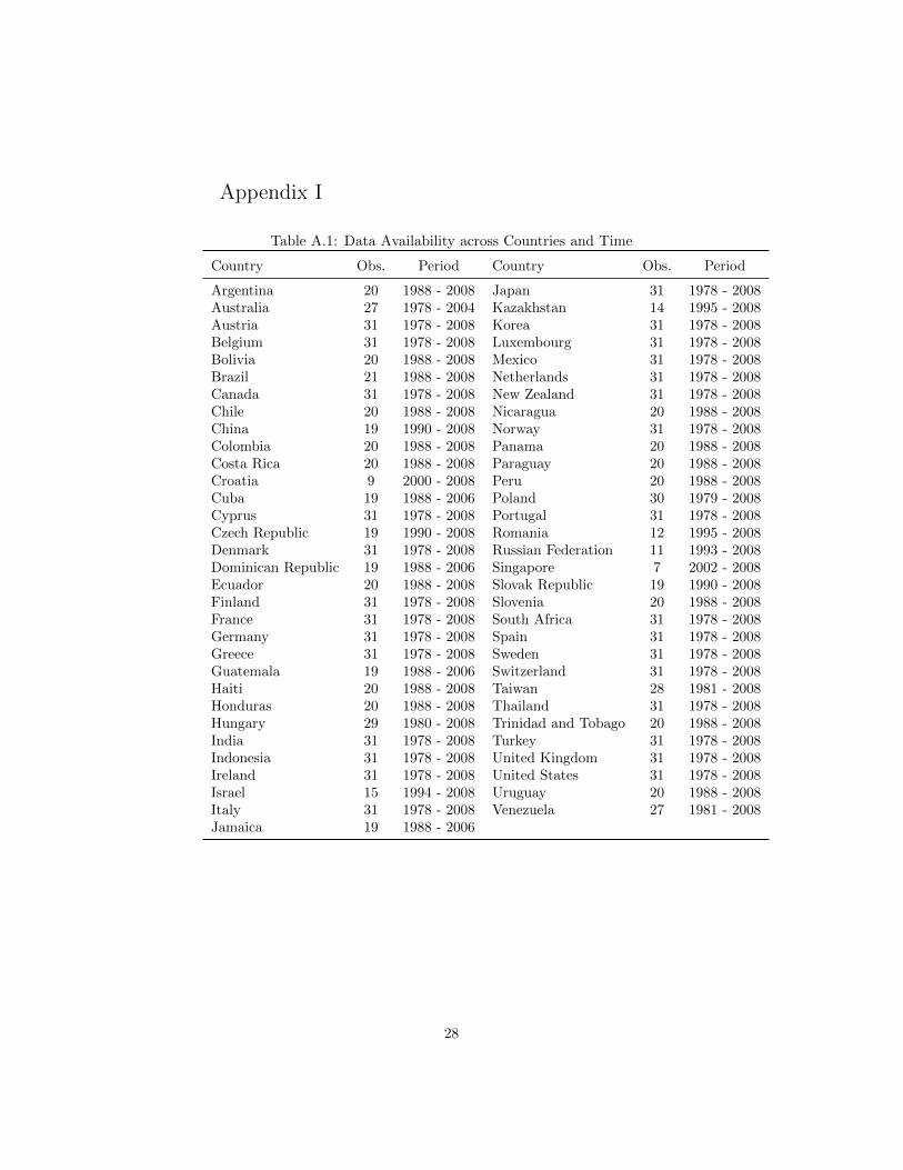
Appendix I
Table A.1: Data Availability across Countries and Time
Country Obs. Period Country Obs. Period
Argentina 20 1988 - 2008 Japan 31 1978 - 2008Australia 27 1978 - 2004 Kazakhstan 14 1995 - 2008Austria 31 1978 - 2008 Korea 31 1978 - 2008Belgium 31 1978 - 2008 Luxembourg 31 1978 - 2008Bolivia 20 1988 - 2008 Mexico 31 1978 - 2008Brazil 21 1988 - 2008 Netherlands 31 1978 - 2008Canada 31 1978 - 2008 New Zealand 31 1978 - 2008Chile 20 1988 - 2008 Nicaragua 20 1988 - 2008China 19 1990 - 2008 Norway 31 1978 - 2008Colombia 20 1988 - 2008 Panama 20 1988 - 2008Costa Rica 20 1988 - 2008 Paraguay 20 1988 - 2008Croatia 9 2000 - 2008 Peru 20 1988 - 2008Cuba 19 1988 - 2006 Poland 30 1979 - 2008Cyprus 31 1978 - 2008 Portugal 31 1978 - 2008Czech Republic 19 1990 - 2008 Romania 12 1995 - 2008Denmark 31 1978 - 2008 Russian Federation 11 1993 - 2008Dominican Republic 19 1988 - 2006 Singapore 7 2002 - 2008Ecuador 20 1988 - 2008 Slovak Republic 19 1990 - 2008Finland 31 1978 - 2008 Slovenia 20 1988 - 2008France 31 1978 - 2008 South Africa 31 1978 - 2008Germany 31 1978 - 2008 Spain 31 1978 - 2008Greece 31 1978 - 2008 Sweden 31 1978 - 2008Guatemala 19 1988 - 2006 Switzerland 31 1978 - 2008Haiti 20 1988 - 2008 Taiwan 28 1981 - 2008Honduras 20 1988 - 2008 Thailand 31 1978 - 2008Hungary 29 1980 - 2008 Trinidad and Tobago 20 1988 - 2008India 31 1978 - 2008 Turkey 31 1978 - 2008Indonesia 31 1978 - 2008 United Kingdom 31 1978 - 2008Ireland 31 1978 - 2008 United States 31 1978 - 2008Israel 15 1994 - 2008 Uruguay 20 1988 - 2008Italy 31 1978 - 2008 Venezuela 27 1981 - 2008Jamaica 19 1988 - 2006
28

Table A.2: Predicted Energy Production across Countries in 2008
Country Coal Gas Oil Country Coal Gas Oil
Argentina No Yes Yes Japan Yes No NoAustralia Yes Yes Yes Kazakhstan Yes Yes YesAustria No Yes No Korea Yes No NoBelgium No No No Luxembourg No No NoBolivia No Yes Yes Mexico Yes Yes YesBrazil Yes Yes Yes Netherlands No Yes YesCanada Yes Yes Yes New Zealand Yes Yes YesChile No Yes No Nicaragua No No NoChina Yes Yes Yes Norway No Yes YesColombia Yes Yes Yes Panama No No NoCosta Rica No No No Paraguay No No NoCroatia No Yes Yes Peru No Yes YesCuba No Yes Yes Poland Yes Yes NoCyprus No No No Portugal No No NoCzech Republic Yes No No Romania Yes Yes YesDenmark No Yes Yes Russian Federation Yes Yes YesDominican Republic No No No Singapore No No NoEcuador No Yes Yes Slovak Republic No No NoFinland No No No Slovenia No No NoFrance Yes No No South Africa Yes Yes NoGermany Yes Yes Yes Spain Yes No NoGreece Yes No No Sweden No No NoGuatemala No No Yes Switzerland No No NoHaiti No No No Taiwan No Yes NoHonduras No No No Thailand Yes Yes YesHungary Yes Yes No Trinidad and Tobago No Yes YesIndia Yes Yes Yes Turkey Yes No YesIndonesia Yes Yes Yes United Kingdom Yes Yes YesIreland No Yes No United States Yes Yes YesIsrael No Yes No Uruguay No No NoItaly No Yes Yes Venezuela Yes Yes YesJamaica No No No
29

Table A.3: Output Change in the Counterfactual and Baseline Simulations usingGTAP-E Model (in USD million)
Industry Counterfactual Simulations Baseline Simulations
Production: Production: Production: Production: Production: Production:All Fuels 1 or 2 Fuels No Fuels All Fuels 1 or 2 Fuels No Fuels
Policy 1: Carbon Tax, $US 30 per ton of CO2
Agriculture -1581 -665 -1833 -1595 -627 -1847Coal -19052 -2141 -401 -16932 -1878 -421Oil -6219 -5422 -710 -6689 -5825 -747Gas -14274 -2671 -1087 -15294 -2754 -1110Oil products -16825 -4146 -355 -17289 -5317 -297Electricity -28432 -6360 -1240 -28896 -6446 -1180En int ind -5749 10519 -16318 -6162 11083 -16329Oth ind ser -28624 -15396 12769 -28756 -14802 12964
Total -120756 -26282 -9175 -121613 -26566 -8967
Policy 2: Removal of Oil Subsidies
Agriculture -1998 -798 -67 -1982 -814 -68Coal -760 -55 -3 -1174 -97 -8Oil -12375 427 384 -11969 713 406Gas -2440 -591 -215 -1844 -586 -205Oil products -45966 -5955 9703 -45481 -5398 9680Electricity -5795 -2883 254 -7854 -3420 234En int ind -9240 -3327 3819 -8889 -3668 3798Oth ind ser -24352 -17022 -4233 -23888 -17280 -4316
Total -102925 -30204 9642 -103082 -30550 9521
Note: Baseline simulations employ fuel substitution elasticities estimated using full sample andreported in column 2 of Table 6. Counterfactual simulations employ fuel substition elasticitiesestimated using region-specific subsamples reported in columns 3, 4, and 5 of Table 6.
30