Embed Size (px)
Citation preview
ORNL/TM-2012/44
Foundation Heat Exchanger Final Report: Demonstration, Measured Performance, and Validated Model and Design Tool
January 2012 Revised January 2013
Prepared by Patrick Hughes Piljae Im Energy and Transportation Science Division Sponsored by Building Technologies Program U.S. Department of Energy
DOCUMENT AVAILABILITY
Reports produced after January 1, 1996, are generally available free via the U.S. Department of Energy (DOE) Information Bridge.
Web site http://www.osti.gov/bridge
Reports produced before January 1, 1996, may be purchased by members of the public from the following source.
National Technical Information Service 5285 Port Royal Road Springfield, VA 22161 Telephone 703-605-6000 (1-800-553-6847) TDD 703-487-4639 Fax 703-605-6900 E-mail [email protected] Web site http://www.ntis.gov/support/ordernowabout.htm Reports are available to DOE employees, DOE contractors, Energy Technology Data Exchange (ETDE) representatives, and International Nuclear Information System (INIS) representatives from the following source.
Office of Scientific and Technical Information P.O. Box 62 Oak Ridge, TN 37831 Telephone 865-576-8401 Fax 865-576-5728 E-mail [email protected] Web site http://www.osti.gov/contact.html
This report was prepared as an account of work sponsored by an agency of the United States Government. Neither the United States Government nor any agency thereof, nor any of their employees, makes any warranty, express or implied, or assumes any legal liability or responsibility for the accuracy, completeness, or usefulness of any information, apparatus, product, or process disclosed, or represents that its use would not infringe privately owned rights. Reference herein to any specific commercial product, process, or service by trade name, trademark, manufacturer, or otherwise, does not necessarily constitute or imply its endorsement, recommendation, or favoring by the United States Government or any agency thereof. The views and opinions of authors expressed herein do not necessarily state or reflect those of the United States Government or any agency thereof.
ORNL/TM-2012/27
Energy and Transportation Science Division
FOUNDATION HEAT EXCHANGER FINAL REPORT:
DEMONSTRATION, MEASURED PERFORMANCE, AND VALIDATED
MODEL AND DESIGN TOOL
Patrick Hughes
Piljae Im
Date Published: January 2012
Revised: January 2013
Prepared by
OAK RIDGE NATIONAL LABORATORY
Oak Ridge, Tennessee 37831-6283
managed by
UT-BATTELLE, LLC
for the
U.S. DEPARTMENT OF ENERGY
under contract DE-AC05-00OR22725

iii
CONTENTS
ACKNOWLEDGMENTS ................................................................................................................... IV
ABBREVIATIONS ............................................................................................................................... V
EXECUTIVE SUMMARY ................................................................................................................... 1
1. INTRODUCTION ............................................................................................................................ 4
2. FIELD TEST OF THE FOUNDATION HEAT EXCHANGER CONCEPT .................................. 7
2.1 Field Test of FHX — One of Many Experiments in the First ZEBRAlliance Project ............... 7
2.2 Description of Houses 1 and 2 .................................................................................................... 7
2.3 Description of Ground Heat Exchangers Installed in Houses 1 and 2 ...................................... 11
2.4 Ground Heat Exchanger Performance Measurements .............................................................. 18
2.5 Measured Performance ............................................................................................................. 24
3. NUMERICAL MODEL AND DESIGN TOOL DEVELOPMENT AND VALIDATION ............ 32
3.1 Objectives and Approach .......................................................................................................... 32
3.2 Research-Grade, 2-Dimensional, Fine-Grid, Finite-Volume, FHX Model .............................. 33
3.3 Research-Grade, Multi-Block, Boundary-Fitted, 3-Dimensional, Finite-Volume, FHX
Model ........................................................................................................................................ 35
3.4 Computationally Efficient, 3-Dimensional, Dual-Coordinate-system, Finite-Volume,
FHX Model ............................................................................................................................... 37
3.5 Practical FHX Design Tool Implemented in Excel .................................................................. 39
3.6 Geographic Range of Feasibility of GSHP Systems Using FHX in the United States ............. 41
4. DISCUSSION ................................................................................................................................. 43
5. REFERENCES ............................................................................................................................... 47
APPENDIX – LIST AND LOCATION OF SENSORS ...................................................................... 49

iv
ACKNOWLEDGMENTS
This report and the work described were sponsored by the Building Technologies Program of the U.S.
Department of Energy’s Office of Energy Efficiency and Renewable Energy and the Tennessee Valley
Authority.
The authors wish especially to acknowledge the contributions of Schaad Companies, which acquired the
land and built the test houses for this research at their own expense, and leased them to ORNL for $1 per
month for the duration of the project. Without Schaad Companies this research project (and many others
utilizing a total of four test houses) would not have been possible. In addition, ClimateMaster, Inc.
donated the water-source heat pumps installed in the test houses and used in the research reported here.
This and other research projects, reliant upon the same test houses but not the subject of this report, also
benefited from contributions of materials and expertise made by additional industry partners of Oak Ridge
National Laboratory, as acknowledged at www.zebralliance.com. ZEBRAlliance — a publicprivate
partnership to maximize cost-effective energy efficiency in buildings — was co-founded by ORNL and
Schaad Companies in 2008.

v
ABBREVIATIONS
2D Two dimensional
3D Three dimensional
ACCA Air Conditioning Contractors of America
ACH Air changes per hour
ASHRAE American Society of Heating, Refrigerating and Air-Conditioning Engineers
CAD Computer-aided design
COP Coefficient of performance
DCS Dual-coordinate system
DOE U.S. Department of Energy
DTN Dynamic thermal network
EER Energy efficiency ratio
EFT Entering fluid temperature
ERV Energy recovery ventilator
EWT Entering water temperature
FHX Foundation heat exchanger
GSHP Ground source heat pump
HERS Home Energy Rating System
HGHX Horizontal ground heat exchanger
HI High insulation
IECC International Energy Conservation Code
LFT Leaving fluid temperature
LWT Leaving water temperature
OA Outdoor air
OAT Outdoor air temperature
ORNL Oak Ridge National Laboratory
OSB Oriented strand board
OSU Oklahoma State University
OVF Optimal value framing
SIP Structural insulated panel
VBA Visual Basic for Applications
VHI Very high insulation
WAHP Water to air heat pump
WWHP Water to water heat pump

vi
1
EXECUTIVE SUMMARY
Geothermal heat pumps, sometimes called ground-source heat pumps (GSHPs), have been proven capable
of significantly reducing energy use and peak demand in buildings. Conventional equipment for
controlling the temperature and humidity of a building, or supplying hot water and fresh outdoor air, must
exchange energy (or heat) with the building’s outdoor environment. Equipment using the ground as a heat
source and heat sink consumes less non-renewable energy (electricity and fossil fuels) because the earth is
cooler than outdoor air in summer and warmer in winter. The most important barrier to rapid growth of
the GSHP industry is high first cost of GSHP systems to consumers.
The most common GSHP system utilizes a closed-loop ground heat exchanger. This type of GSHP
system can be used almost anywhere. There is reason to believe that reducing the cost of closed-loop
systems is the strategy that would achieve the greatest energy savings with GSHP technology. The cost
premium of closed-loop GSHP systems over conventional space conditioning and water heating systems
is primarily associated with drilling boreholes or excavating trenches, installing vertical or horizontal
ground heat exchangers, and backfilling the excavations.
This project investigates reducing the cost of horizontal closed-loop ground heat exchangers by installing
them in the construction excavations, augmented when necessary with additional trenches. This approach
applies only to new construction of residential and light commercial buildings or additions to such
buildings. In the business-as-usual scenario, construction excavations are not used for the horizontal
ground heat exchanger (HGHX); instead the HGHX is installed entirely in trenches dug specifically for
that purpose. The potential cost savings comes from using the construction excavations for the installation
of ground heat exchangers, thereby minimizing the need and expense of digging additional trenches.
The term foundation heat exchanger (FHX) has been coined to refer exclusively to ground heat
exchangers installed in the overcut around the basement walls. The primary technical challenge
undertaken by this project was the development and validation of energy performance models and design
tools for FHX. In terms of performance modeling and design, ground heat exchangers in other
construction excavations (e.g., utility trenches) are no different from conventional HGHX, and models
and design tools for HGHX already exist.
This project successfully developed and validated energy performance models and design tools so that
FHX or hybrid FHX/HGHX systems can be engineered with confidence, enabling this technology to be
applied in residential and light commercial buildings. The validated energy performance model also
addresses and solves another problem, the longstanding inadequacy in the way ground–building thermal
interaction is represented in building energy models, whether or not there is a ground heat exchanger
nearby.
Two side-by-side, three-level, unoccupied research houses with walkout basements, identical 3,700 ft2
floor plans, and hybrid FHX/HGHX systems were constructed to provide validation data sets for the
energy performance model and design tool. The envelopes of both houses are very energy efficient and
airtight, and the HERS ratings of the homes are 44 and 45 respectively. Both houses are mechanically
ventilated with energy recovery ventilators, with space conditioning provided by water-to-air heat pumps
with 2 ton nominal capacities. Separate water-to-water heat pumps with 1.5 ton nominal capacities were
used for water heating. In these unoccupied research houses, human impact on energy use (hot water draw,
etc.) is simulated to match the national average.
At House 1 the hybrid FHX/HGHX system was installed in 300 linear feet of excavation, and 60% of that
was construction excavation (needed to construct the home). At House 2 the hybrid FHX/HGHX system
was installed in 360 feet of excavation, 50% of which was construction excavation. There are six pipes in

2
all excavations (three parallel circuits – out and back), and the multiple instances of FHX and/or HGHX
are all connected in series. The working fluid is 20% by weight propylene glycol in water.
Model and design tool development was undertaken in parallel with constructing the houses, installing
instrumentation, and monitoring performance for a year. Several detailed numerical models for FHX were
developed as part of the project. Essentially the project team was searching for an energy performance
model accurate enough to achieve project objectives while also having sufficient computational efficiency
for practical use in EnergyPlus. A 3-dimensional, dual-coordinate-system, finite-volume model satisfied
these criteria and was included in the October 2011 EnergyPlus Version 7 public release after being
validated against measured data. EnergyPlus using this model can complete an annual simulation of an
FHX thermally coupled to a basement in less than two minutes on a standard desktop computer.
A practical design tool for sizing pure FHX or hybrid FHX/HGHX systems was also developed and
implemented in Excel using Visual Basic for Applications. Using the design tool, sizing the FHX or
FHX/HGHX for a residential application can be accomplished in about five minutes. Compared to one of
the numerical models, the design tool was found to oversize the ground heat exchanger by 17 to 20% in
five of six benchmarking locations, and by 29% in the remaining location. The design tool oversized the
hybrid FHX/HGHX system at House 1 by 23%. Given the inherent uncertainties in design inputs such as
building loads and soil thermal properties, this level of accuracy in a simplified FHX design method is
acceptable.
One of the numerical models was used to investigate the geographical range of technical feasibility of
FHX systems. Preliminary analysis indicated that pure FHX systems are technically feasible for new
construction in nearly half the United States. Although not investigated, hybrid FHX/HGHX systems
using all available construction excavations should have some level of installed cost savings over
conventional HGHX systems in almost any residential or light commercial new construction project
involving significant excavation. Since FHX and hybrid FHX/HGHX ground heat exchangers are
designed to maintain the same operating temperature range as conventional ground heat exchangers, the
energy-savings performance of the GSHP system is the same regardless, making cost reduction the
primary goal.
Preliminary estimates indicate that when implemented at scale by a production builder, ground heat
exchanger in construction excavations (FHX in overcut around basement or HGHX in utility trenches)
may be feasible at $1,000 per ton. That compares with traditional vertical-loop and six-pipe-per-virgin-
trench HGHX systems that typically are installed in East Tennessee at $3,000 per ton and $2,250 per ton,
respectively. If these values are correct, hybrid systems would warrant consideration even when use of
construction excavations exclusively is not feasible. For example, a 3-ton hybrid FHX/HGHX ground
heat exchanger application where construction excavations are adequate for two-thirds of the load would
cost $4,250 (2 x $1000 + $2,250) compared to $6,750 (3 x $2,250) for pure HGHX in virgin trench. The
actual cost of a particular project may vary depending on drilling/trenching conditions, regional cost
variations, underground soil thermal properties and building geometry. Whether cost reductions through
use of construction excavations are enough for GSHP systems to gain significantly broader consideration
in new construction markets remains to be seen. The authors recommend several next steps to find out.

3
4
1. INTRODUCTION
Geothermal heat pumps, sometimes called ground-source heat pumps (GSHPs), have been proven capable
of significantly reducing energy use and peak demand in buildings. Conventional equipment for
controlling the temperature and humidity of a building, or supplying hot water and fresh outdoor air, must
exchange energy (or heat) with the building’s outdoor environment. Equipment using the ground as a heat
source and heat sink consumes less non-renewable energy (electricity and fossil fuels) because the earth is
cooler than outdoor air in summer and warmer in winter. Heat pumps are always used in GSHP systems.
They efficiently move heat from ground energy sources or to ground heat sinks as needed. Although heat
pumps consume electrical energy, they move 3 to 5 times as much energy between the building and the
ground than they consume while doing so.
Policy makers are seeking clean energy technology options that can be deployed with speed and scale to
provide large reductions in building energy use. The most important barrier to rapid growth of the GSHP
industry is high first cost of GSHP systems to consumers (Hughes 2008). The most common GSHP
system utilizes a closed-loop ground heat exchanger. This type of GSHP system can be used almost
anywhere, regardless of the availability or suitability of nearby surface water, gray water, effluent, storm
water, rainwater, or groundwater. Since the number of GSHP systems installed can have a dramatic
impact on first cost to consumers (shipment volume begets affordability), there is reason to believe that
reducing the cost of closed-loop systems is the strategy that would achieve the greatest energy savings
with GSHP technology. The cost premium of closed-loop GSHP systems over conventional space
conditioning and water heating systems is primarily associated with drilling boreholes or excavating
trenches, installing vertical or horizontal ground heat exchangers, and backfilling the excavations.
In general, the length of the bore or excavation needed for a given building is a function of the building’s
space conditioning and water heating loads. Minimizing those loads minimizes the ground heat exchanger
size and the excavation needed for its installation. In the case of extremely energy efficient homes and
light commercial buildings, space conditioning and water heating loads may be so low that the
excavations required to construct the buildings provide sufficient space by themselves for the entire
length of ground heat exchanger. But even when insufficient for the entire ground heat exchanger, using
the construction excavations minimizes the need for additional trenching and reduces costs. The
construction excavations are already bought and paid for — why not use them for double duty?
This project investigates reducing the cost of horizontal closed-loop ground heat exchangers by installing
them in the construction excavations, augmented when necessary with additional trenches. In general,
construction excavations may include the overcut around the basement walls, below the basement floor,
utility trenches (for buried water, sewer, and power), and trenches for draining the foundation footers. The
term foundation heat exchanger (FHX) has been coined to refer exclusively to ground heat exchangers
installed in the overcut around basement walls. The primary technical challenge undertaken by this
project was the development and validation of energy models and design tools for FHX. In terms of
performance modeling and design, ground heat exchangers in utility and footer drain trenches are no
different from conventional horizontal ground heat exchangers (HGHX), and models and design tools for
HGHX already exist. When trenches are used for double duty, adequate spacing is of course required
(e.g., between buried water lines and heat exchanger loops), but simple guidance on this issue is expected
to suffice.
Ground heat exchangers installed below the basement floor are not addressed in this report. Project
resources were insufficient to address both FHX and sub-floor systems, and it was important to tackle the
greatest technical challenge first. Since the sub-floor case has very simple geometry and boundary
conditions, the project team felt confident that this capability could be added to the models and design

5
tools later. As it turned out, the computationally efficient performance model developed by this project is
able to model sub-floor systems, although this capability has not yet been validated against measured
data.
A previous project successfully demonstrated that a GSHP system using construction excavations was
feasible for a specific, small, ultra-high-energy-efficiency house in one climate (Christian and Bonar
2008). The project documented in this report developed and validated performance models and design
tools so that FHX or hybrid FHX/HGHX systems can be engineered with confidence, hence enabling the
technology to be applied on a large scale.
In this day of scarce research and development resources, it is always important to design research
projects to solve multiple problems wherever possible. Another problem addressed and solved here is the
longstanding inadequacy in the way ground–building thermal interaction is represented in building energy
models. Today’s flagship building energy models (DOE-2, EnergyPlus, etc.) were originally designed
with large commercial buildings in mind, and it is understandable that not much attention was paid to
ground–building thermal interaction. Compared to many other large building characteristics at the time,
this feature had only a small influence on predicted building energy consumption. Recently, however,
there has been much greater emphasis on using energy models as an integrated whole-building design tool,
and mandatory energy codes and voluntary rating systems are driving higher levels of building energy
efficiency. In addition, usability of these models has improved, and their use in light commercial and even
residential projects is growing — hence ground–building thermal interaction is no longer negligible. The
numerical models developed by this project accurately characterize ground–building thermal interaction,
whether or not there is a ground heat exchanger nearby.
Oak Ridge National Laboratory (ORNL) assembled a team for the project that included Schaad
Companies, one of the largest home builders in East Tennessee, and a team led by Dr. Jeff Spitler of
Oklahoma State University (OSU) and including Dr. Simon Rees (De Montfort University, United
Kingdom) and several post-graduate students. ORNL provided the overall project management during the
multi-year effort. ORNL’s role included providing Schaad Companies with technical expertise and access
to ORNL’s industry partners during the design and construction of two test homes having GSHP systems
using hybrid FHX/HGHX, developing the FHX/HGHX test plan, installing the instrumentation,
collecting and analyzing performance data, defining the technical scope of work for the OSU subcontract,
managing the OSU subcontract, and authoring this final report. ORNL’s research effort was sponsored by
the U.S. Department of Energy (DOE) Building Technologies Program and Tennessee Valley Authority.
Schaad Companies (schaadcompanies.com), ORNL’s founding partner in ZEBRAlliance — a public-
private partnership to maximize cost-effective energy efficiency in buildings (zebralliance.com) — has
built four energy-efficient test houses in the Crossroads at Wolf Creek Subdivision in Oak Ridge,
Tennessee. Schaad Companies acquired the land and built the test houses at their own expense, and leased
them for $1 per month each to ORNL for research purposes for 30 months. Houses 1 and 2, which were
used for the FHX research, are three-level homes with walkout basements. Houses 1 and 2 were
completed in November 2009 and data collection began in December.
OSU’s relationship to ORNL was that of a research subcontractor. The funding for the OSU subcontract
was provided to ORNL by the DOE Building Technologies Program. OSU engaged De Montfort
University through a sub-tier agreement. The role of the OSU team was to develop (1) a research-grade,
2-dimensional, fine-grid, finite-volume FHX energy model in HVACSIM+, (2) a research-grade, multi-
block, boundary-fitted, 3-dimensional, finite-volume FHX energy model in EnergyPlus, (3) a
computationally efficient, 3-dimensional, dual-coordinate-system, finite-volume, FHX energy model in
EnergyPlus, and (4) a practical FHX and hybrid FHX/HGHX design tool implemented in Excel using
Visual Basic for Applications (VBA). The OSU role also included using the measured data from the test
house provided by ORNL to validate the various FHX energy models and the practical design tool,

6
integrating a validated FHX model into a whole-building energy simulation of a single-family residence,
and using simulation to explore the geographic range of feasibility of GSHP systems using pure FHX
ground heat exchangers in single-family residences in the United States.
This report documents the overall project in a brief and easily readable format and cites other publications
where the project’s technical work is documented in great detail. In the special case of the test house field
data acquisition and analysis, the detailed documentation is included in the body and appendices of this
report since it exists nowhere else.

7
2. FIELD TEST OF THE FOUNDATION HEAT EXCHANGER CONCEPT
2.1 Field Test of FHX — One of Many Experiments in the First ZEBRAlliance Project
ORNL and Schaad Companies founded the ZEBRAlliance in August 2008 through Memorandum of
Agreement MOA-UTB-2008037 and a separate alliance agreement. ZEBRAlliance is a public-private
partnership to maximize the cost-effective energy efficiency of buildings. As part of the first
ZEBRAlliance project, Schaad Companies built four energy-efficient test houses in the Crossroads at
Wolf Creek Subdivision in Oak Ridge, Tennessee. Schaad Companies acquired the land and built the test
houses at their own expense, and leased them for $1 per month each to ORNL for research purposes for
30 months. Another member of the alliance, BarberMcMurry Architects, donated their time to design the
test houses. More than 30 ORNL industry partners became alliance members and donated their most
advanced energy efficiency products for use in the construction. The four ZEBRAlliance test houses are
being used for many different experiments. For more information, visit www.zebralliance.com.
2.2 Description of Houses 1 and 2
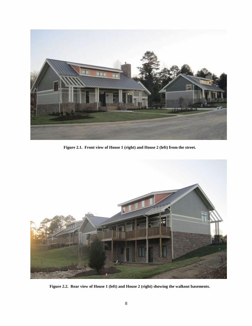
The side-by-side research houses, House 1 and House 2, have identical 3,700 ft2 floor plans. In these
unoccupied research houses, human impact on energy use is simulated to match the national average, with
showers, lights, ovens, washers, and other energy-consuming equipment turned on and off at exactly the
same times. Simulating occupancy eliminates a major source of uncertainty in whole-house energy
consumption, enabling valid side-by-side experiments even when each “case” has a sample size of one.
The primary experiment using houses 1 and 2 involved testing two different envelope strategies — a
structural insulated panel (SIP) envelope in House 1, and an Optimal Value Framing (OVF) envelope in
House 2. As implemented, both of these strategies had very low air leakage and high levels of insulation,
and thus have very low heat gain and loss through the building envelope, which of course contributes to
their very low space conditioning loads. In short, they are exactly the type of homes where it should be
feasible to install a large portion of the ground heat exchanger in construction excavations. Figures 2.1
and 2.2 show front and rear views of the houses.
The ground heat exchangers in houses 1 and 2 (described in Section 2.3) were intentionally similar to
provide experimental redundancy, essentially guaranteeing that experimental data would be available to
validate the models and design tools described in Chapter 3. Validation was based on the House 1 data set
for reasons explained later.
The envelope characteristics of House 1 and House 2 are described in detail in Miller et al. 2010.
Summary descriptions of the building envelope subsystems are provided in Table 2.1. It should be noted
that the basement walls are poured concrete with a polymer-enhanced asphalt membrane spray-applied to
the outside for waterproofing. Fiberglass 2⅜ in. drainage board is placed against and adhered to the
asphalt membrane. The drainage board serves dual purposes of insulating the outside of the basement wall
and acting as a drainage plane to enable rainwater to seep to the footer drains.
8
Figure 2.1. Front view of House 1 (right) and House 2 (left) from the street.
Figure 2.2. Rear view of House 1 (left) and House 2 (right) showing the walkout basements.
9
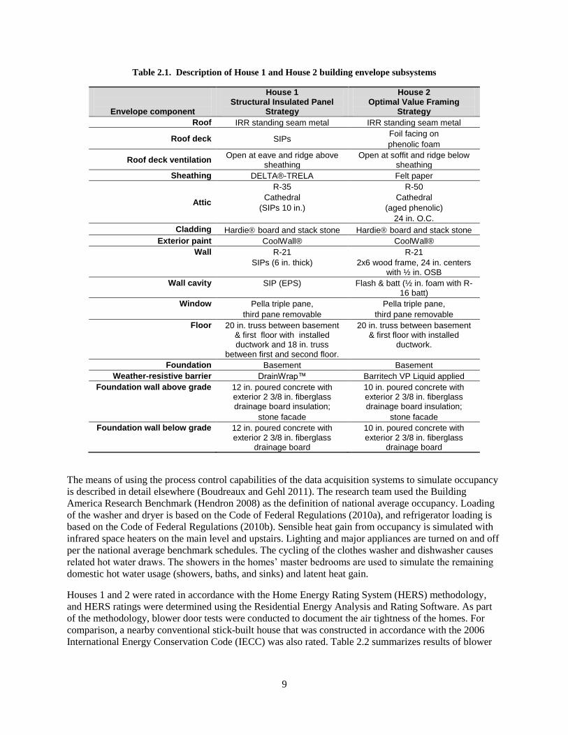
Table 2.1. Description of House 1 and House 2 building envelope subsystems
Envelope component
House 1 Structural Insulated Panel
Strategy
House 2 Optimal Value Framing
Strategy
Roof IRR standing seam metal IRR standing seam metal
Roof deck SIPs Foil facing on
phenolic foam
Roof deck ventilation Open at eave and ridge above
sheathing Open at soffit and ridge below
sheathing
Sheathing DELTA®-TRELA Felt paper
Attic
R-35
Cathedral
(SIPs 10 in.)
R-50
Cathedral
(aged phenolic)
24 in. O.C.
Cladding Hardie board and stack stone Hardie board and stack stone
Exterior paint CoolWall® CoolWall®
Wall R-21
SIPs (6 in. thick)
R-21
2x6 wood frame, 24 in. centers with ½ in. OSB
Wall cavity SIP (EPS) Flash & batt (½ in. foam with R-16 batt)
Window Pella triple pane,
third pane removable
Pella triple pane,
third pane removable
Floor 20 in. truss between basement & first floor with installed ductwork and 18 in. truss
between first and second floor.
20 in. truss between basement & first floor with installed
ductwork.
Foundation Basement Basement
Weather-resistive barrier DrainWrap™ Barritech VP Liquid applied
Foundation wall above grade 12 in. poured concrete with exterior 2 3/8 in. fiberglass drainage board insulation;
stone facade
10 in. poured concrete with exterior 2 3/8 in. fiberglass drainage board insulation;
stone facade
Foundation wall below grade 12 in. poured concrete with exterior 2 3/8 in. fiberglass
drainage board
10 in. poured concrete with exterior 2 3/8 in. fiberglass
drainage board
The means of using the process control capabilities of the data acquisition systems to simulate occupancy
is described in detail elsewhere (Boudreaux and Gehl 2011). The research team used the Building
America Research Benchmark (Hendron 2008) as the definition of national average occupancy. Loading
of the washer and dryer is based on the Code of Federal Regulations (2010a), and refrigerator loading is
based on the Code of Federal Regulations (2010b). Sensible heat gain from occupancy is simulated with
infrared space heaters on the main level and upstairs. Lighting and major appliances are turned on and off
per the national average benchmark schedules. The cycling of the clothes washer and dishwasher causes
related hot water draws. The showers in the homes’ master bedrooms are used to simulate the remaining
domestic hot water usage (showers, baths, and sinks) and latent heat gain.
Houses 1 and 2 were rated in accordance with the Home Energy Rating System (HERS) methodology,
and HERS ratings were determined using the Residential Energy Analysis and Rating Software. As part
of the methodology, blower door tests were conducted to document the air tightness of the homes. For
comparison, a nearby conventional stick-built house that was constructed in accordance with the 2006
International Energy Conservation Code (IECC) was also rated. Table 2.2 summarizes results of blower
10
door tests and HERS ratings for House 1 and House 2 compared to the stick-built “builder house” that
complies with IECC 2006.
Table 2.2. Comparison of HERS ratings and infiltration rates of House 1 (SIP house),
House 2 (OVF house), and “Builder House”
House 1 House 2 Builder Housea
ACH @ 50 Pab 1.23 1.74 5.7
HERSc 46 47 101
aBuilt to comply with IECC 2006.
bAir changes per hour (ACH) measured by blower door tests conducted at pressurization of 50 Pa.
cHome Energy Rating System (HERS) – lower numbers indicate greater energy efficiency.
Houses 1 and 2 are intentionally very air tight and require mechanical ventilation to satisfy ASHRAE
Standard 62.2. To satisfy this requirement, each house is outfitted with an energy recovery ventilator
(ERV), whose operation and performance characteristics are described in detail elsewhere (Fantech
2010).
The space cooling and heating design loads for houses 1 and 2 were calculated using “Manual J:
Residential Load Calculation” and associated software tools developed by the Air Conditioning
Contractors of America (ACCA). The space conditioning design load calculations included consideration
of the impact of ERV mechanical ventilation. The calculated design heating and total (sensible plus latent)
cooling loads were 32,698 kBtu/h and 23,954 kBtu/h respectively for House 1, and 34,037 kBtu/h and
23,813 kBtu/h for House 2.
Space conditioning in houses 1 and 2 is provided by water-to-air heat pumps (WAHPs) connected to
ground heat exchangers (combination of FHX and conventional HGHX, as described later). The WAHPs
were sized using ACCA’s “Manual S: Residential Equipment Selection” methodology as it applies to
WAHPs. Nominal 2 ton capacity units with two-stage compressors were selected for both House 1 and
House 2. For comparison, typically in East Tennessee, a house built to code and having 3,700 ft2 of floor
space would require a 4 to 5 ton nominal capacity unit for space conditioning (Im, Liu, and Monk 2011).
Supplemental electric resistance heat was also installed.
It should be noted that both houses have multi-zone forced air distribution systems. Separate zone
thermostats are provided for the master bedroom, the rest of the main floor living area, the upstairs, and
the basement, for a total of four zones. The fact that the distribution systems are multi-zone on the air side
does not influence space conditioning design loads or WAHP equipment selection, since the Manual J and
Manual S methodologies are based on the whole-building block loads.
As noted previously, houses 1 and 2 are unoccupied research houses where the hot water usage is
simulated to match the national average (54 gallons per day for these houses) as defined by the Building
America Benchmark. The hot water systems in houses 1 and 2 are identical and comprised of a storage
tank whose set temperature is maintained by a water-to-water heat pump (WWHP) connected to the same
combination of FHX and HGHX used for space conditioning. The WWHPs selected were 1½ ton nominal
capacity with integral recirculation pumps for both the source and load sides. On the source side the
WWHPs are equipped with a control valve to limit the maximum leaving fluid temperature to 65oF.
11
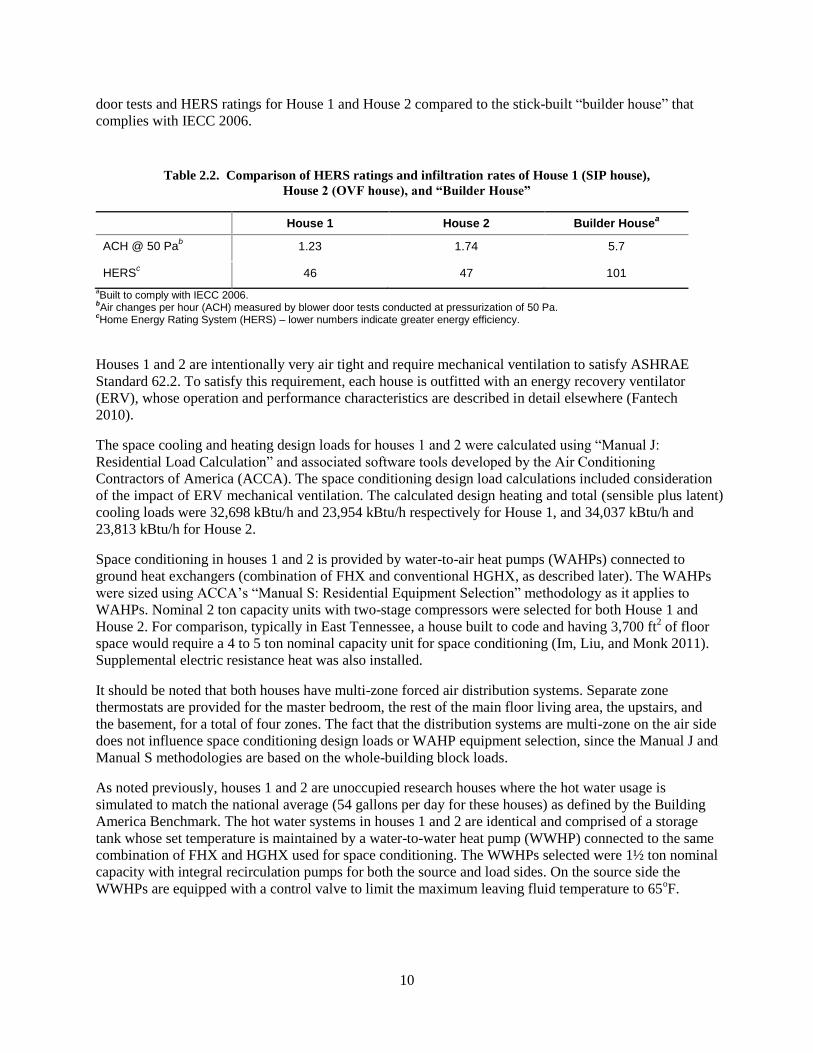
Figure 2.3 is a photo of the WAHP and WWHP with associated hot water storage tank as installed in
House 1. The equipment installation in House 2 is identical. The characteristics of the WAHP and
WWHP units are summarized in Table 2.3.
Figure 2.3. Space conditioning equipment (WAHP on right) and water heating equipment (WWHP
and associated tank on left) at House 1.
2.3 Description of Ground Heat Exchangers Installed in Houses 1 and 2
In general, ground heat exchangers may be installed in the overcut around the basement walls, below the
basement floor, in utility trenches (for buried water, sewer, and power lines), and in trenches for draining
the footers. Depending on the application, the contractor may include extra trench in the design for
installation of conventional horizontal ground heat exchangers (HGHX). This research project focused on
the greatest technical challenge, which was developing and validating models and design tools for FHX
inserted into the overcut around basement walls. In terms of performance modeling and design, ground
heat exchangers in utility and footer drain trenches are no different from HGHX in supplemental trenches,
and models and design tools for HGHX already exist. This project did not explicitly address models and
design tools for ground heat exchangers installed below the basement floor, because that configuration
has very simple geometry and boundary conditions, and we felt that this capability could be developed
and added to the models and design tools later. We use the term FHX to refer exclusively to ground heat
exchanger in the overcut around basement walls, and the term HGHX to refer to ground heat exchanger in
utility, footer drain, or supplemental trenches.
12
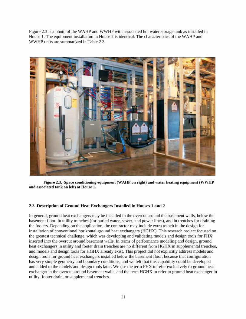
Table 2.3. Characteristics of WAHP and WWHP systems installed in House 1 and House 2
WAHP WWHP
Performance Metrics
EFTa Range 20-120°F 20-110°F
Capacity 2 ton (nominal) 1.5 ton (nominal)
COP Coolingb
5.4 (full load) at sink EFT = 77°F 7.6 (part load) at sink EFT = 68°F
Heatingc
4.0 (full load) at source EFT = 32°F 4.6 (part load) at source EFT = 41°F
Heating at source EFT = 68°F: 5.2 for 90°F load EFT 3.7 for 120°F load EFT
Heating at source EFT = 32°F: 3.5 for 90°F load EFT 2.5 for 120°F load EFT
Airflow Cooling: 850 CFM rated (full load) 725 CFM rated (part load)
Heating: 950 CFM rated (full load) 825 CFM rated (part load)
NA
Fluid flow rate – ground heat exchanger side
1.5 gpm/ton 5.0 gpm (maximum)
Modulating valve maintains LFT
d below 65
oF
HW flow rate NA 3.5 gpm
Other Salient Features
Size, in. (W × H × D) 22.4 × 48.5 × 25.6 24 × 23.5 × 24.5
Weight 266 lb 166 lb
Air coils Electro-coated to protect against corrosion, airborne dust buildup, etc.
NA
Compressor Copeland Scroll UltraTech™
Two-stage: 67% part-load capacity step
LG™ high-efficiency rotary
single stage
Blower Wheel (Dia × W): 9 × 7 in. NA
Blower motor Variable speed GE ECM Half speed (1/2 hp) [373 W] Full speed (1 hp) [746 W]
NA
Current RLA Compressor Blower motor Pump
10.3 Amps 4.3 Amps 0.8 Amps
6.6 Amps 0.43 Amps
Ground loop fluid 20% propylene glycol (by weight) in water
20% propylene glycol (by weight) in water
Refrigerant HFC- 410A 58 oz. charge
HFC- 410A 56 oz. charge
aEFT = entering fluid temperature (entering heat pump from ground heat exchanger).
bCooling coefficient of performance (COP) at 80.6°F (27°C) DB, 66.2°F (19°C) WB entering air temperature.
cHeating coefficient of performance (COP) at 68°F (20°C) DB, 59° (15°C) WB entering air temperature.
dLFT = leaving fluid temperature (entering ground heat exchanger from heat pump).
The primary objective of the experiment, then, was to generate experimental data for FHX inserted into
the overcut around basement walls, so that energy performance models and design tools for FHX in this
configuration can be validated against the measured data. Further, it is desirable that the models and
design tools have the flexibility to address applications where the ground heat exchanger may be
comprised of a combination of FHX and HGHX. Hence, having a hybrid FHX/HGHX experimental
system was an advantage.

13
It is apparent from Figure 2.2 that the basement walls at the back of houses 1 and 2 are above grade and
not available for FHX, and that each house has a basement wall with marginal usefulness for FHX
because of a sloped grade. Hence the FHX was installed only along the two basement walls bounded by a
full-depth and level grade — the north (street side) and west walls. The rest of the ground heat exchanger
is HGHX installed in utility and supplemental trenches.
As no FHX design tool was available at the time, the team used a design tool for sizing conventional
HGHX loops as a guide, and then applied engineering judgment. The team selected a six-pipe
configuration, meaning six ¾ inch diameter high-density polyethylene pipes in the excavations (three
fluid circuits – out and back) with a minimum spacing of 1 ft between pipes. The soil thermal
conductivity assumed was 0.75 Btu/(hr·ft·F). Maximum and minimum heat pump entering fluid
temperatures (EFTs) of 95F and 30F were used as the design constraints for sizing the ground heat
exchanger. The necessary design values for heat extraction from the ground during winter and heat
rejection to the ground during summer were derived from the space conditioning and water heating loads,
and efficiency of equipment satisfying those loads, using a bin analysis.
It was estimated that 300 feet of excavation would be required for House 1. The north and west basement
walls are 46 ft and 34 ft long, respectively, for a total of 80 ft. Since the pipe follows the outside perimeter
of the overcut excavation, which is longer than the actual basement wall due to features such as the
fireplace and the outside corner between the north and west basement walls, the effective FHX excavation
length is approximately 100 ft (as determined by the 3D CAD model described in Section 2.4). The
remaining 200 ft of required excavation was provided in the form of utility or supplemental trenches.
The layout of the ground heat exchanger at House 1 (the SIP House) is illustrated in Figure 2.4. The
trench for the buried electrical service entrance (northeast or upper right) provides 30 ft of the 200 ft
required. The trench for the supply water connection (Southwest or lower left) provided 50 ft of the 200 ft
required. The remaining required HGHX is installed south of the house. Although part of this HGHX
segment is labeled “rain garden,” the data show that a “rain garden” performs the same as the equivalent
amount of six-pipe horizontal trench (i.e., the trench length required to accommodate the same amount of
pipe as was installed in the rain garden). The equivalent length of six-pipe trench (in the rain garden or
not) south of the house provides the remaining 120 ft of the 200 ft required. In other words, 60% (180 of
300 ft) of the excavations used for installation of the ground heat exchanger were required anyway to
construct the home.
14
Figure 2.4. Layout of the FHX and HGHX at House 1.
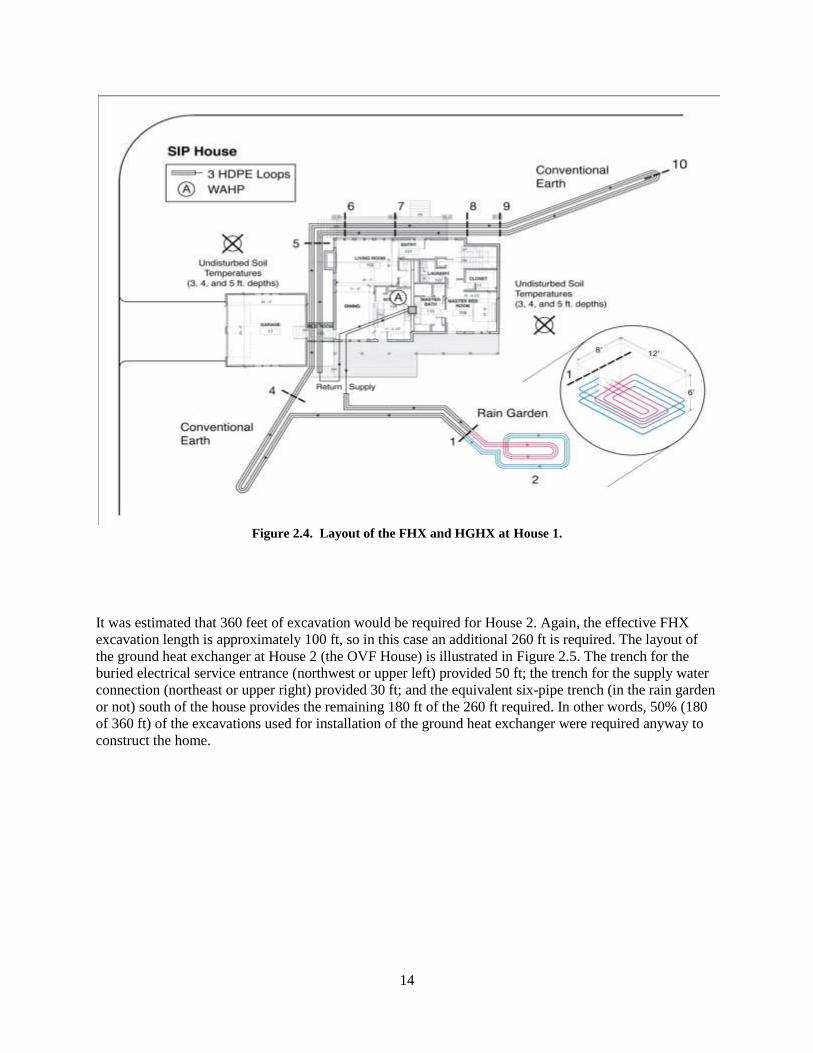
It was estimated that 360 feet of excavation would be required for House 2. Again, the effective FHX
excavation length is approximately 100 ft, so in this case an additional 260 ft is required. The layout of
the ground heat exchanger at House 2 (the OVF House) is illustrated in Figure 2.5. The trench for the
buried electrical service entrance (northwest or upper left) provided 50 ft; the trench for the supply water
connection (northeast or upper right) provided 30 ft; and the equivalent six-pipe trench (in the rain garden
or not) south of the house provides the remaining 180 ft of the 260 ft required. In other words, 50% (180
of 360 ft) of the excavations used for installation of the ground heat exchanger were required anyway to
construct the home.
15
Figure 2.5. Layout of the FHX and HGHX at House 2.
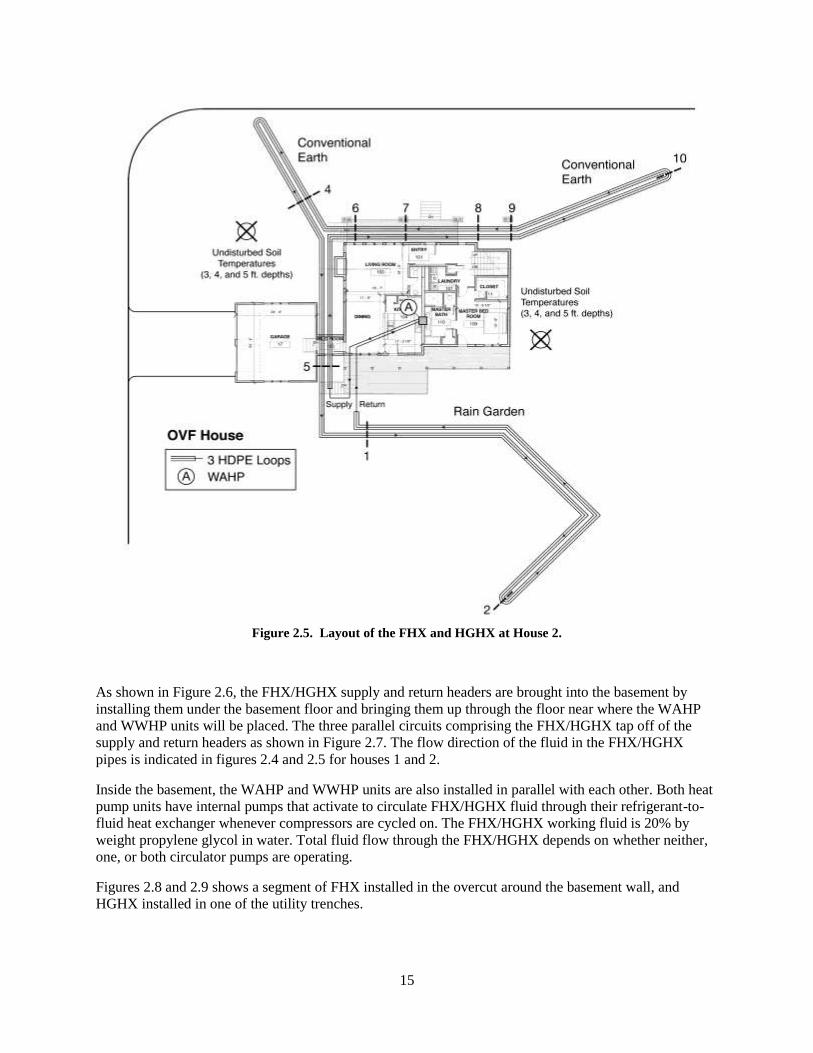
As shown in Figure 2.6, the FHX/HGHX supply and return headers are brought into the basement by
installing them under the basement floor and bringing them up through the floor near where the WAHP
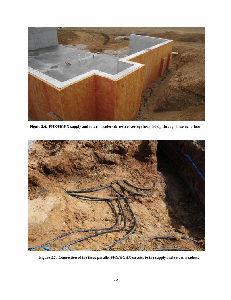
and WWHP units will be placed. The three parallel circuits comprising the FHX/HGHX tap off of the
supply and return headers as shown in Figure 2.7. The flow direction of the fluid in the FHX/HGHX
pipes is indicated in figures 2.4 and 2.5 for houses 1 and 2.
Inside the basement, the WAHP and WWHP units are also installed in parallel with each other. Both heat
pump units have internal pumps that activate to circulate FHX/HGHX fluid through their refrigerant-to-
fluid heat exchanger whenever compressors are cycled on. The FHX/HGHX working fluid is 20% by
weight propylene glycol in water. Total fluid flow through the FHX/HGHX depends on whether neither,
one, or both circulator pumps are operating.
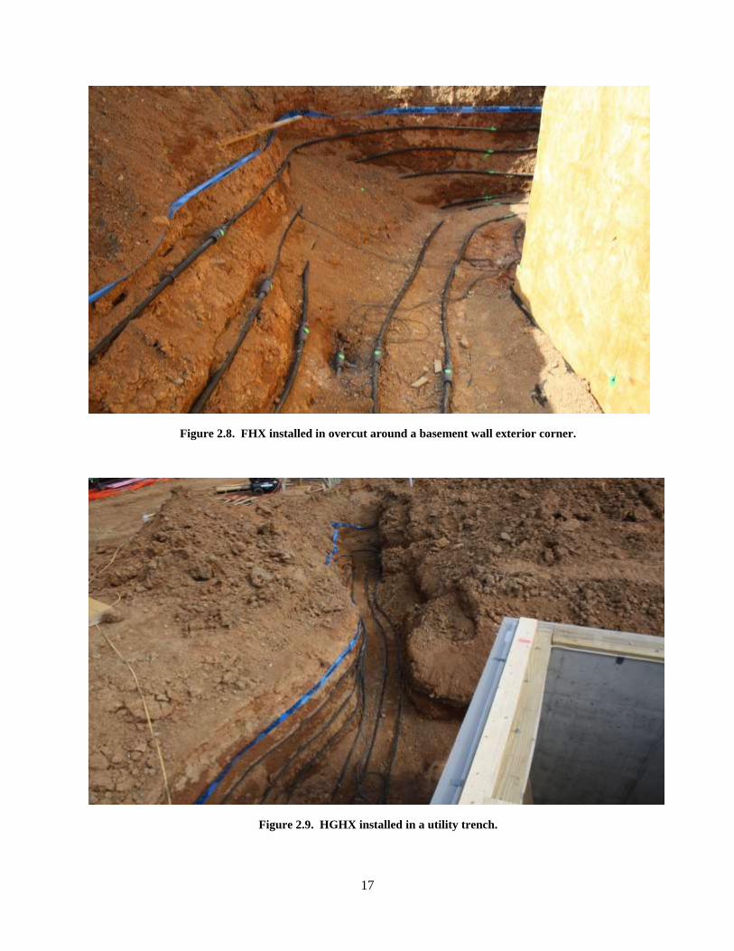
Figures 2.8 and 2.9 shows a segment of FHX installed in the overcut around the basement wall, and
HGHX installed in one of the utility trenches.
16
Figure 2.6. FHX/HGHX supply and return headers (brown covering) installed up through basement floor.
Figure 2.7. Connection of the three parallel FHX/HGHX circuits to the supply and return headers.
17
Figure 2.8. FHX installed in overcut around a basement wall exterior corner.
Figure 2.9. HGHX installed in a utility trench.
18
2.4 Ground Heat Exchanger Performance Measurements
Measurements taken to establish FHX/HGHX performance and enable model validation included the
thermal loads (heat rejection and extraction) imposed by the equipment, undisturbed far field temperature
of the soil at various depths, numerous temperatures on the outside surface of the pipes, basement wall
heat flux, drainage board and near-wall soil temperatures in a few locations, soil thermal conductivity,
and weather data at the demonstration site.
The manufacturer of the WAHP and WWHP units installed a differential pressure transducer across the
fluid side of the internal fluid-to-refrigerant heat exchanger and used factory turbine flow meter
measurements to generate calibration curves for heat exchanger pressure drop vs. ground heat exchanger
flow rate at several entering fluid temperature (EFT) values. These software-implemented calibration
curves enabled fluid flow rate through the unit to be deduced from the pressure drop measurement during
the field experiment. The valve modulating the fluid flow through the WWHP unit can result in very low
flows under some operating conditions and insufficient measurement accuracy of the flow rate using the
calibration curve approach. Therefore a redundant turbine flow meter measurement was included in the
field experiment. Since the WAHP and WWHP were plumbed in parallel, the total FHX/HGHX fluid
flow rate equaled the sum of the fluid flow rates through the separate units.
The manufacturer also installed thermal wells on the inlet and outlet of the fluid side of the internal fluid-
to-refrigerant heat exchanger. The thermal wells were used for fluid temperature measurements during the
field experiment. Heat rejection to, or extraction from, the FHX/HGHX was deduced from the
measurements of fluid flow rate and inlet and outlet fluid temperatures whenever the WAHP and WWHP
compressors were operating. Appropriate corrections were applied during data reduction to account for
the working fluid being 20% propylene glycol by weight in water, rather than pure water.
Undisturbed far field soil temperature measurements were taken at two different locations at 3, 4, and 5 ft
depths at houses 1 and 2. The locations of these measurements are shown in figures 2.4 and 2.5. The
temperature measurements were made with thermistors that were carefully calibrated prior to installation.
Fluid temperatures along the FHX/HGHX pipes were approximated by measuring the outside pipe
surface temperature of all six pipes at nine different locations, numbered as 1, 2, 4, 5, 6, 7, 8, 9, and 10
(the number 3 was not used) in figures 2.4 and 2.5. Again, all temperature measurements were made with
thermistors that were carefully calibrated prior to installation. The thermistors were applied directly to the
outside of the pipes and then wrapped with insulation. Green dots were applied to the insulation over the
thermistor locations to facilitate use of photogrammetric techniques (described later in this section) to
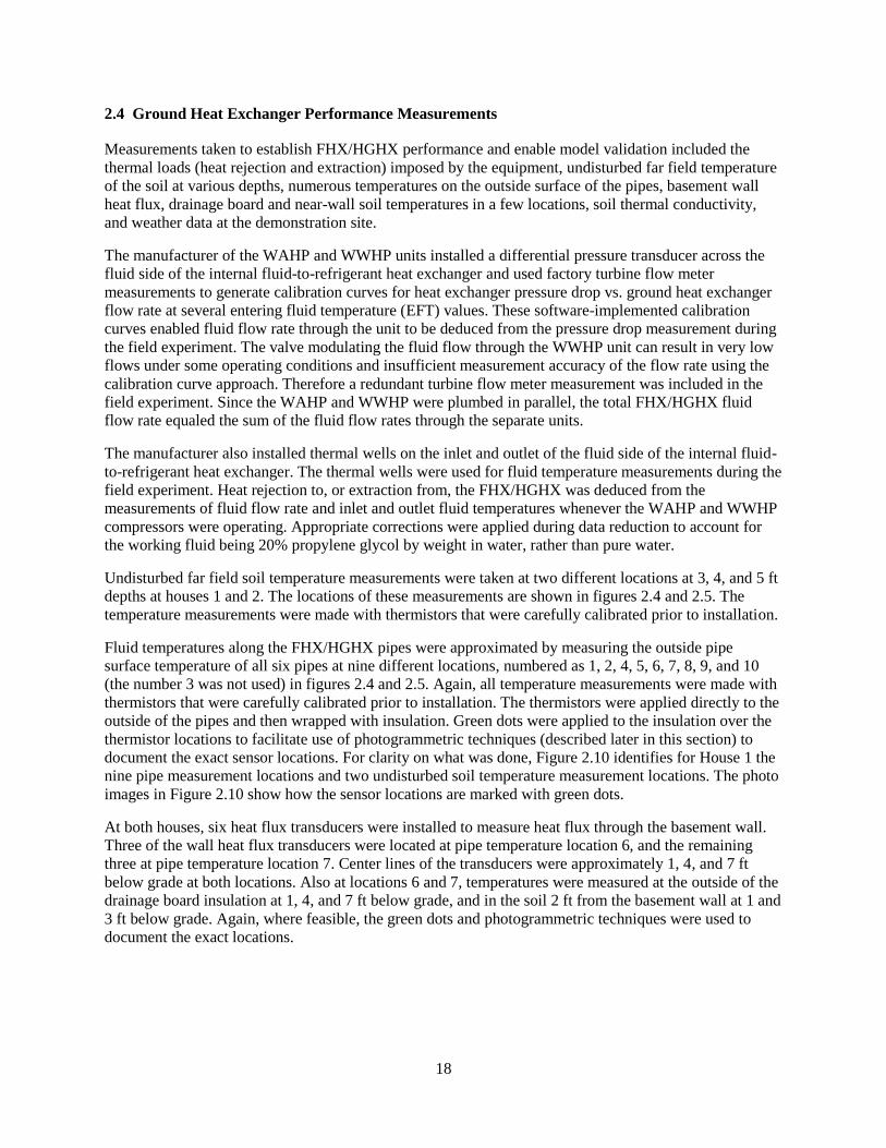
document the exact sensor locations. For clarity on what was done, Figure 2.10 identifies for House 1 the
nine pipe measurement locations and two undisturbed soil temperature measurement locations. The photo
images in Figure 2.10 show how the sensor locations are marked with green dots.
At both houses, six heat flux transducers were installed to measure heat flux through the basement wall.
Three of the wall heat flux transducers were located at pipe temperature location 6, and the remaining
three at pipe temperature location 7. Center lines of the transducers were approximately 1, 4, and 7 ft
below grade at both locations. Also at locations 6 and 7, temperatures were measured at the outside of the
drainage board insulation at 1, 4, and 7 ft below grade, and in the soil 2 ft from the basement wall at 1 and
3 ft below grade. Again, where feasible, the green dots and photogrammetric techniques were used to
document the exact locations.
19
Figure 2.10. Location of pipe and undisturbed far field soil temperature sensors at House 1.
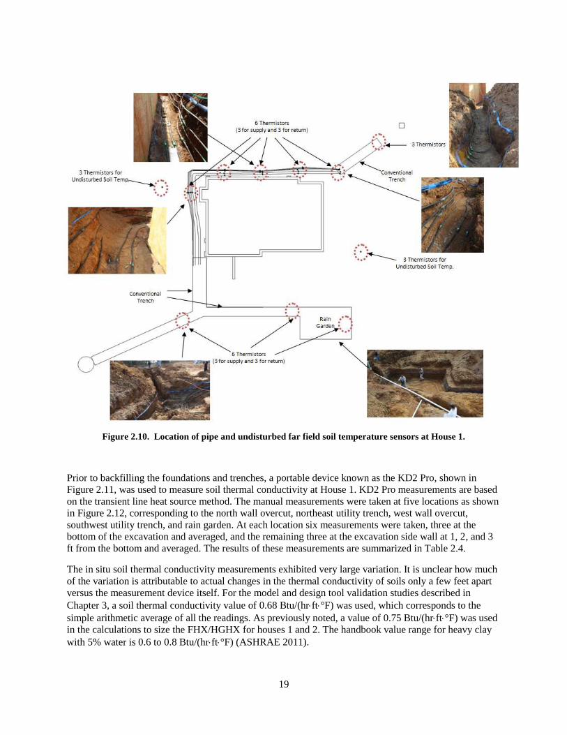
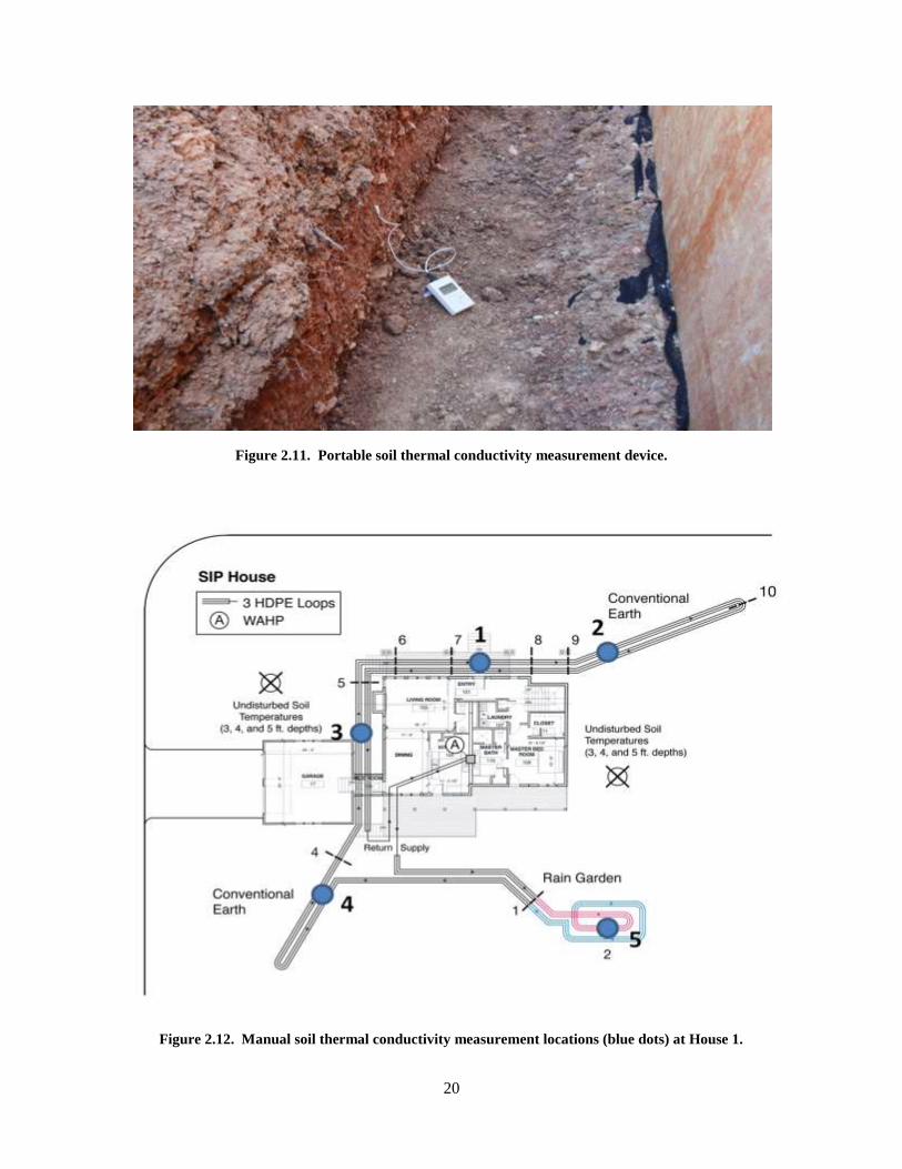
Prior to backfilling the foundations and trenches, a portable device known as the KD2 Pro, shown in
Figure 2.11, was used to measure soil thermal conductivity at House 1. KD2 Pro measurements are based
on the transient line heat source method. The manual measurements were taken at five locations as shown
in Figure 2.12, corresponding to the north wall overcut, northeast utility trench, west wall overcut,
southwest utility trench, and rain garden. At each location six measurements were taken, three at the
bottom of the excavation and averaged, and the remaining three at the excavation side wall at 1, 2, and 3
ft from the bottom and averaged. The results of these measurements are summarized in Table 2.4.
The in situ soil thermal conductivity measurements exhibited very large variation. It is unclear how much
of the variation is attributable to actual changes in the thermal conductivity of soils only a few feet apart
versus the measurement device itself. For the model and design tool validation studies described in
Chapter 3, a soil thermal conductivity value of 0.68 Btu/(hrft°F) was used, which corresponds to the
simple arithmetic average of all the readings. As previously noted, a value of 0.75 Btu/(hrft°F) was used
in the calculations to size the FHX/HGHX for houses 1 and 2. The handbook value range for heavy clay
with 5% water is 0.6 to 0.8 Btu/(hrft°F) (ASHRAE 2011).
20
Figure 2.11. Portable soil thermal conductivity measurement device.
Figure 2.12. Manual soil thermal conductivity measurement locations (blue dots) at House 1.
21
Table 2.4. Summary of in-situ soil thermal conductivity measurement results (Btu/(hr·ft·°F))
Location of Measurement
Measured spot 1
North wall 2
Utility trench 3
West wall 4
Utility trench 5
Rain garden
Bottom – average 0.44 0.23 0.64 0.90 0.58
Wall – average 0.98 0.86 0.67 0.88 0.61
In order to use the FHX/HGHX data to validate the models and design tool, it was critical to know the
exact location of ground heat exchanger piping, temperature sensors, heat flux transducers, and other
features in relation to the basement walls. Given the nature of construction sites, it was expected that the
excavations would take irregular shapes, making it difficult to document the actual geometry of what was
installed. In addition, the location of pipes and sensors cannot be determined after the excavations are
backfilled. For this reason, photogrammetric techniques that allow the spatial location of objects to be
determined from photographs were used to develop an accurate geometric model of the FHX/HGHX and
foundations. PhotoModeler, a software tool which helps to create accurate, high-quality, three-
dimensional (3D) models and measurements from photographs using an ordinary camera, was used for
this purpose. (More information on this general technique and the PhotoModeler tool are available at
http://www.photomodeler.com.)
In the simplest example, the 3D coordinates of points on an object are determined from measurements
made on two or more photographic images taken from different angles. When common points are
identified on each image, a line of sight can be constructed from the camera location to the point on the
object. The intersection of these rays then determines the 3D location of the point. For each important
feature, certain key reference points and reference lengths were identified. For example, numbered
stickers were affixed to the ground heat exchanger piping at three-foot intervals. Further, the previously
mentioned green dots were affixed to each sensor location. Photographs of the foundations and the piping
were then taken from multiple angles around the site. Based on the photographs, the software interpreted
these key reference points and lengths and produced a 3D CAD model of the FHX/HGHX and
foundations.
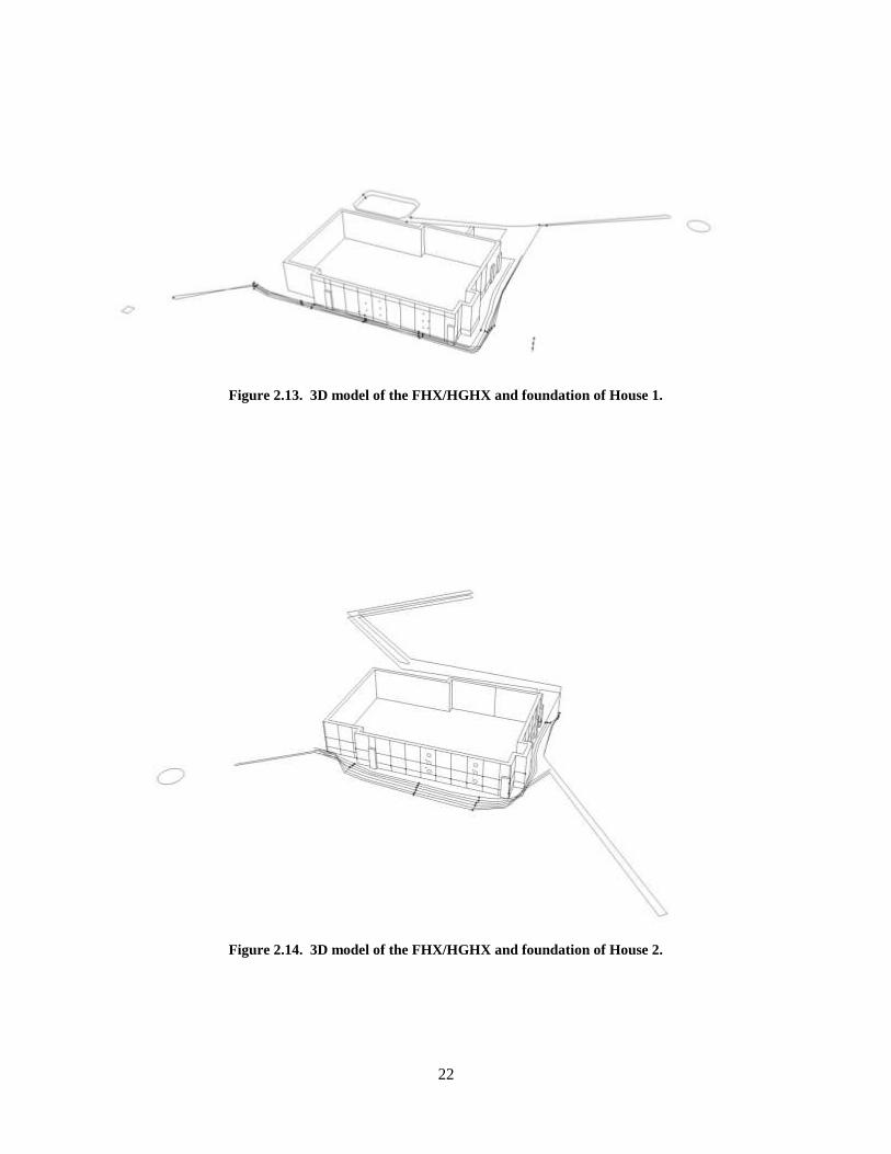
Figures 2.13 and 2.14 show the final 3D CAD models of houses 1 and 2, respectively. In these models,
the six pipes (three for supply and three for return) and the sensors for the FHX in the overcuts around the
basement walls were modeled individually, whereas the conventional HGHX is modeled as one line for
each three pipes, whether supply or return.
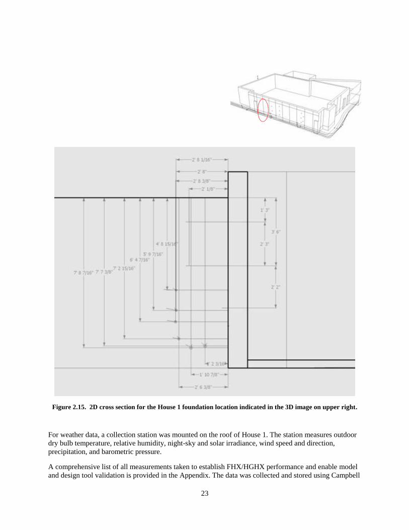
Based on the 3D CAD models, one can easily determine the 2D coordinates locating features such as the
basement wall, FHX pipes, and sensors on pipes for a specific cross section perpendicular to the pipe and
basement wall. By manually outputting multiple 2D cross sections and averaging them, the 3D CAD
model was used to determine the average coordinates of these features along the entire length of the north
and west basement walls having FHX. This capability was extremely useful for model validation using
the measured data. An example of a 2D cross section generated by the 3D model appears in Figure 2.15.
22
Figure 2.13. 3D model of the FHX/HGHX and foundation of House 1.
Figure 2.14. 3D model of the FHX/HGHX and foundation of House 2.
23
Figure 2.15. 2D cross section for the House 1 foundation location indicated in the 3D image on upper right.
For weather data, a collection station was mounted on the roof of House 1. The station measures outdoor
dry bulb temperature, relative humidity, night-sky and solar irradiance, wind speed and direction,
precipitation, and barometric pressure.
A comprehensive list of all measurements taken to establish FHX/HGHX performance and enable model
and design tool validation is provided in the Appendix. The data was collected and stored using Campbell
24
Scientific Model CR3000 micro-loggers and retrieved remotely over dedicated telephone lines. Frequent
data retrieval enabled the project team to have early warning of data channel malfunctions so that any
issues could be resolved quickly. In general the data is measured at a rapid scan rate with averages logged
at 15 minute intervals, but some channels were logged at intervals as short as 1 minute as necessary.
2.5 Measured Performance
The WAHP and WWHP units were replaced by prototypes of a new ground-source integrated heat pump
in December 2010, which interrupted data collection. Hence all of the measured performance reported
here is for January through November 2010. However, eleven months was an ample data set for deriving
accurate analytical approaches (e.g., empirical models) to estimate values for December 2010, enabling
performance results to be reported for a full year.
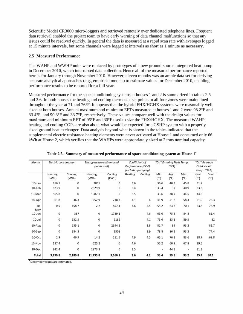
Measured performance for the space conditioning systems at houses 1 and 2 is summarized in tables 2.5
and 2.6. In both houses the heating and cooling thermostat set points in all four zones were maintained
throughout the year at 71 and 76°F. It appears that the hybrid FHX/HGHX systems were reasonably well
sized at both houses. Annual maximum and minimum EFTs measured at houses 1 and 2 were 93.2°F and
33.4°F, and 90.3°F and 33.7°F, respectively. These values compare well with the design values for
maximum and minimum EFT of 95°F and 30°F used to size the FHX/HGHX. The measured WAHP
heating and cooling COPs are also about what would be expected for a GSHP system with a properly
sized ground heat exchanger. Data analysis beyond what is shown in the tables indicated that the
supplemental electric resistance heating elements were never activated at House 1 and consumed only 66
kWh at House 2, which verifies that the WAHPs were appropriately sized at 2 tons nominal capacity.
Table 2.5. Summary of measured performance of space conditioning system at House 1
a
Month Electric consumption Energy delivered/removed (loads met)
Coefficient of Performance (COP) (includes pumping)
“On” Entering Fluid Temp. (EFT)
“On” Average Outdoor Air Temp. (OAT)
Heating (kWh)
Cooling (kWh)
Heating (kWh)
Cooling (KWh)
Heating Cooling Min (°F)
Avg. (°F)
Max. (°F)
Heat (°F)
Cool (°F)
10-Jan 856.1 0 3051 0 3.6 36.6 40.3 45.8 31.7
10-Feb 823.9 0 2829.9 0 3.4 33.4 37 40.9 33.3
10-Mar 565.8 0 1987.1 0 3.5 33.6 38.7 44.5 44.5
10-Apr 61.8 36.3 252.9 218.3 4.1 6 41.9 51.2 58.4 51.9 76.3
10-May
0.5 158.7 2.2 857.1 4.6 5.4 55.2 63.8 70.1 53.8 75.9
10-Jun 0 387 0 1789.1 4.6 65.6 75.8 84.8 81.4
10-Jul 0 532.5 0 2182 4.1 75.6 83.8 89.5 82
10-Aug 0 635.1 0 2394.1 3.8 81.7 89 93.2 81.7
10-Sep 0 384.3 0 1508 3.9 78.8 86.2 93.2 77.4
10-Oct 2.9 46.9 14.2 211.5 4.9 4.5 65.1 76.1 83.6 38.7 69.8
10-Nov 137.4 0 625.2 0 4.6 55.2 60.9 67.8 39.5
10-Dec 842.4 0 2973.3 0 3.5 - 44.8 - 31.3
Total 3,290.8 2,180.8 11,735.8 9,160.1 3.6 4.2 33.4 59.8 93.2 35.4 80.1
a December values are estimated.
25
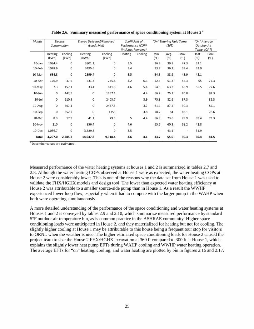
Table 2.6. Summary measured performance of space conditioning system at House 2 a
Month Electric Consumption
Energy Delivered/Removed (Loads Met)
Coefficient of Performance (COP) (Includes Pumping)
“On” Entering Fluid Temp. (EFT)
“On” Average Outdoor Air Temp. (OAT)
Heating (kWh)
Cooling (kWh)
Heating (kWh)
Cooling (kWh)
Heating Cooling Min (°F)
Avg. (°F)
Max. (°F)
Heat (°F)
Cool (°F)
10-Jan 1084.4 0 3801.1 0 3.5 36.8 39.8 47.3 32.1
10-Feb 1028.6 0 3495.6 0 3.4 33.7 36.2 39.4 33.9
10-Mar 684.8 0 2399.4 0 3.5 34.3 38.9 43.9 45.1
10-Apr 126.9 37.6 531.3 235.8 4.2 6.3 42.5 51.3 56.3 55 77.3
10-May 7.3 157.1 33.4 841.8 4.6 5.4 54.8 63.3 68.9 55.5 77.6
10-Jun 0 442.5 0 1967.1 4.4 66.2 75.1 80.8 82.3
10-Jul 0 610.9 0 2403.7 3.9 75.8 82.6 87.3 82.3
10-Aug 0 667.1 0 2437.5 3.7 81.9 87.2 90.3 82.1
10-Sep 0 352.2 0 1353 3.8 78.2 84 88.1 78.6
10-Oct 8.3 17.9 41.1 79.5 5 4.4 66.8 73.6 79.9 39.4 73.3
10-Nov 210 0 956.4 0 4.6 55.5 60.3 68.2 42.8
10-Dec 1,056.7 0 3,689.5 0 3.5 - 43.1 - 31.9
Total 4,207.0 2,285.3 14,947.8 9,318.4 3.6 4.1 33.7 55.0 90.3 36.4 81.5
a December values are estimated.
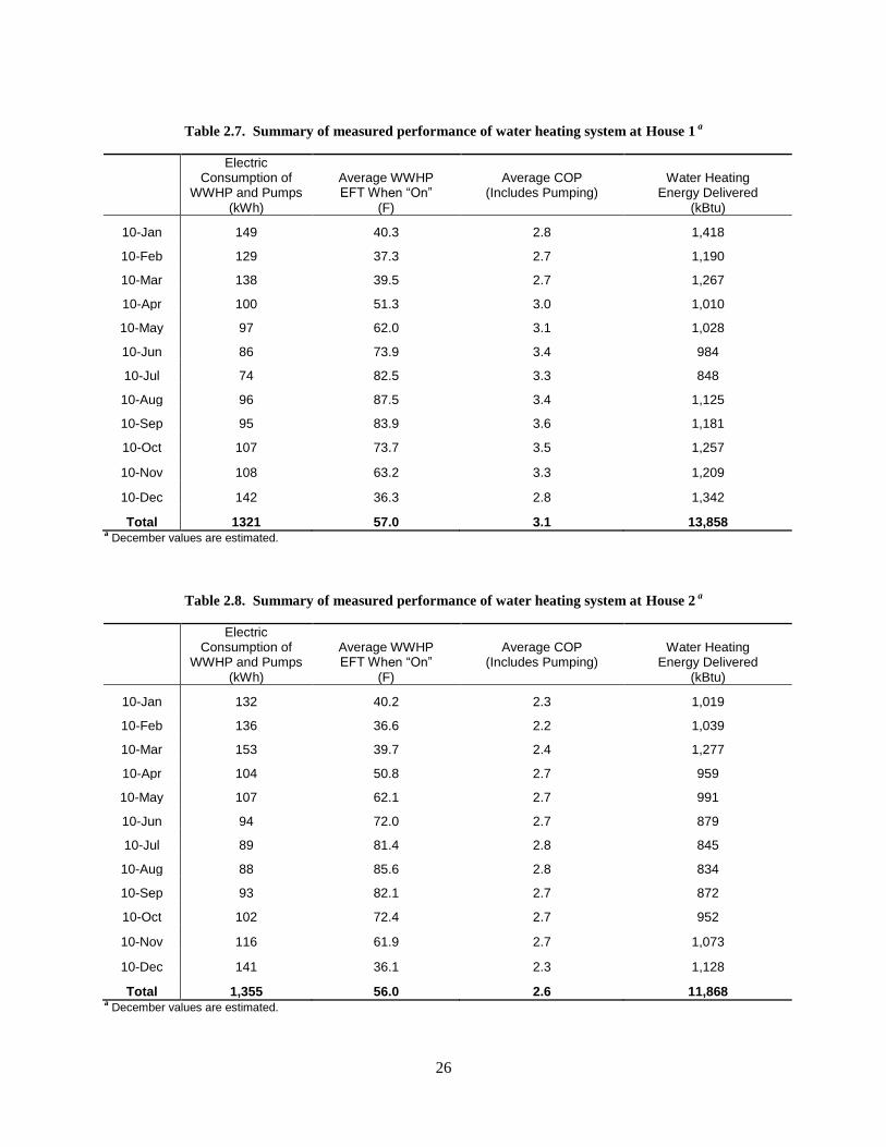
Measured performance of the water heating systems at houses 1 and 2 is summarized in tables 2.7 and
2.8. Although the water heating COPs observed at House 1 were as expected, the water heating COPs at
House 2 were considerably lower. This is one of the reasons why the data set from House 1 was used to
validate the FHX/HGHX models and design tool. The lower than expected water heating efficiency at
House 2 was attributable to a smaller source-side pump than in House 1. As a result the WWHP
experienced lower loop flow, especially when it had to compete with the larger pump in the WAHP when
both were operating simultaneously.
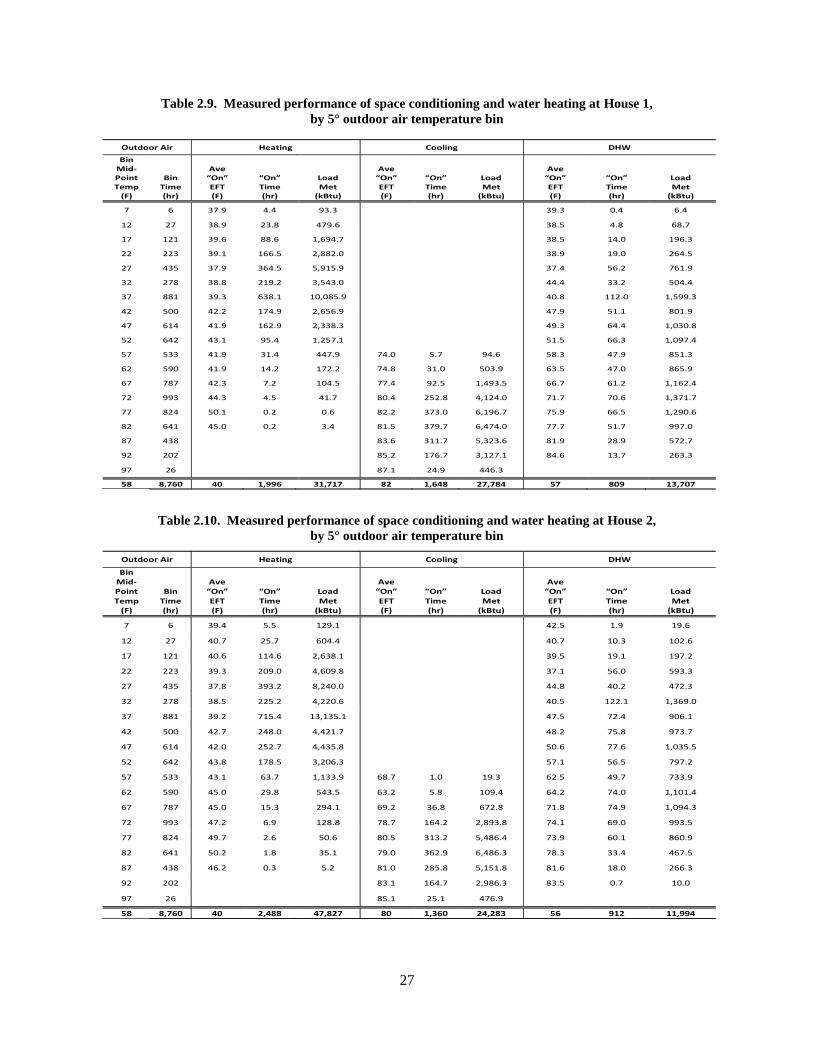
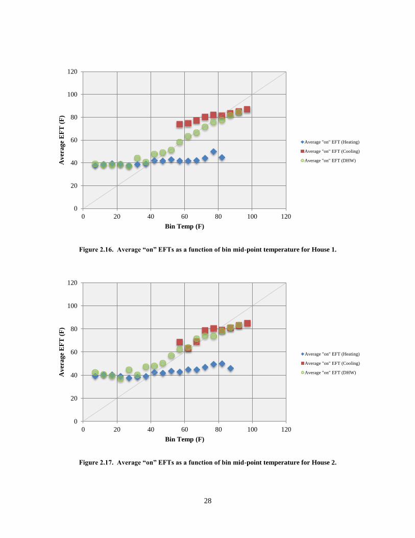
A more detailed understanding of the performance of the space conditioning and water heating systems at
Houses 1 and 2 is conveyed by tables 2.9 and 2.10, which summarize measured performance by standard
5°F outdoor air temperature bin, as is common practice in the ASHRAE community. Higher space
conditioning loads were anticipated in House 2, and they materialized for heating but not for cooling. The
slightly higher cooling at House 1 may be attributable to this house being a frequent tour stop for visitors
to ORNL when the weather is nice. The higher estimated space conditioning loads for House 2 caused the
project team to size the House 2 FHX/HGHX excavation at 360 ft compared to 300 ft at House 1, which
explains the slightly lower heat pump EFTs during WAHP cooling and WWHP water heating operation.
The average EFTs for “on” heating, cooling, and water heating are plotted by bin in figures 2.16 and 2.17.
26
Table 2.7. Summary of measured performance of water heating system at House 1
a
Electric Consumption of
WWHP and Pumps (kWh)
Average WWHP EFT When “On”
(F)
Average COP (Includes Pumping)
Water Heating Energy Delivered
(kBtu)
10-Jan 149 40.3 2.8 1,418
10-Feb 129 37.3 2.7 1,190
10-Mar 138 39.5 2.7 1,267
10-Apr 100 51.3 3.0 1,010
10-May 97 62.0 3.1 1,028
10-Jun 86 73.9 3.4 984
10-Jul 74 82.5 3.3 848
10-Aug 96 87.5 3.4 1,125
10-Sep 95 83.9 3.6 1,181
10-Oct 107 73.7 3.5 1,257
10-Nov 108 63.2 3.3 1,209
10-Dec 142 36.3 2.8 1,342
Total 1321 57.0 3.1 13,858 a December values are estimated.
Table 2.8. Summary of measured performance of water heating system at House 2 a
Electric Consumption of
WWHP and Pumps (kWh)
Average WWHP EFT When “On”
(F)
Average COP (Includes Pumping)
Water Heating Energy Delivered
(kBtu)
10-Jan 132 40.2 2.3 1,019
10-Feb 136 36.6 2.2 1,039
10-Mar 153 39.7 2.4 1,277
10-Apr 104 50.8 2.7 959
10-May 107 62.1 2.7 991
10-Jun 94 72.0 2.7 879
10-Jul 89 81.4 2.8 845
10-Aug 88 85.6 2.8 834
10-Sep 93 82.1 2.7 872
10-Oct 102 72.4 2.7 952
10-Nov 116 61.9 2.7 1,073
10-Dec 141 36.1 2.3 1,128
Total 1,355 56.0 2.6 11,868 a December values are estimated.
27
Table 2.9. Measured performance of space conditioning and water heating at House 1,
by 5° outdoor air temperature bin
Table 2.10. Measured performance of space conditioning and water heating at House 2,
by 5° outdoor air temperature bin
Outdoor Air Heating Cooling DHW
Bin Mid- Point Temp
(F)
Bin Time (hr)
Ave “On” EFT (F)
“On” Time (hr)
Load Met
(kBtu)
Ave “On” EFT (F)
“On” Time (hr)
Load Met
(kBtu)
Ave “On” EFT (F)
“On” Time (hr)
Load Met
(kBtu)
7 6 37.9 4.4 93.3
39.3 0.4 6.4
12 27 38.9 23.8 479.6
38.5 4.8 68.7
17 121 39.6 88.6 1,694.7
38.5 14.0 196.3
22 223 39.1 166.5 2,882.0
38.9 19.0 264.5
27 435 37.9 364.5 5,915.9
37.4 56.2 761.9
32 278 38.8 219.2 3,543.0
44.4 33.2 504.4
37 881 39.3 638.1 10,085.9
40.8 112.0 1,599.3
42 500 42.2 174.9 2,656.9
47.9 51.1 801.9
47 614 41.9 162.9 2,338.3
49.3 64.4 1,030.8
52 642 43.1 95.4 1,257.1
51.5 66.3 1,097.4
57 533 41.9 31.4 447.9 74.0 5.7 94.6 58.3 47.9 851.3
62 590 41.9 14.2 172.2 74.8 31.0 503.9 63.5 47.0 865.9
67 787 42.3 7.2 104.5 77.4 92.5 1,493.5 66.7 61.2 1,162.4
72 993 44.3 4.5 41.7 80.4 252.8 4,124.0 71.7 70.6 1,371.7
77 824 50.1 0.2 0.6 82.2 373.0 6,196.7 75.9 66.5 1,290.6
82 641 45.0 0.2 3.4 81.5 379.7 6,474.0 77.7 51.7 997.0
87 438
83.6 311.7 5,323.6 81.9 28.9 572.7
92 202
85.2 176.7 3,127.1 84.6 13.7 263.3
97 26
87.1 24.9 446.3
58 8,760 40 1,996 31,717 82 1,648 27,784 57 809 13,707
Outdoor Air Heating Cooling DHW
Bin Mid- Point Temp
(F)
Bin Time (hr)
Ave “On” EFT (F)
“On” Time (hr)
Load Met
(kBtu)
Ave “On” EFT (F)
“On” Time (hr)
Load Met
(kBtu)
Ave “On” EFT (F)
“On” Time (hr)
Load Met
(kBtu)
7 6 39.4 5.5 129.1
42.5 1.9 19.6
12 27 40.7 25.7 604.4
40.7 10.3 102.6
17 121 40.6 114.6 2,638.1
39.5 19.1 197.2
22 223 39.3 209.0 4,609.8
37.1 56.0 593.3
27 435 37.8 393.2 8,240.0
44.8 40.2 472.3
32 278 38.5 225.2 4,220.6
40.5 122.1 1,369.0
37 881 39.2 715.4 13,135.1
47.5 72.4 906.1
42 500 42.7 248.0 4,421.7
48.2 75.8 973.7
47 614 42.0 252.7 4,435.8
50.6 77.6 1,035.5
52 642 43.8 178.5 3,206.3
57.1 56.5 797.2
57 533 43.1 63.7 1,133.9 68.7 1.0 19.3 62.5 49.7 733.9
62 590 45.0 29.8 543.5 63.2 5.8 109.4 64.2 74.0 1,101.4
67 787 45.0 15.3 294.1 69.2 36.8 672.8 71.8 74.9 1,094.3
72 993 47.2 6.9 128.8 78.7 164.2 2,893.8 74.1 69.0 993.5
77 824 49.7 2.6 50.6 80.5 313.2 5,486.4 73.9 60.1 860.9
82 641 50.2 1.8 35.1 79.0 362.9 6,486.3 78.3 33.4 467.5
87 438 46.2 0.3 5.2 81.0 285.8 5,151.8 81.6 18.0 266.3
92 202
83.1 164.7 2,986.3 83.5 0.7 10.0
97 26
85.1 25.1 476.9
58 8,760 40 2,488 47,827 80 1,360 24,283 56 912 11,994
28
Figure 2.16. Average “on” EFTs as a function of bin mid-point temperature for House 1.
Figure 2.17. Average “on” EFTs as a function of bin mid-point temperature for House 2.
0
20
40
60
80
100
120
0 20 40 60 80 100 120
Av
era
ge
EF
T (
F)
Bin Temp (F)
Average "on" EFT (Heating)
Average "on" EFT (Cooling)
Average "on" EFT (DHW)
0
20
40
60
80
100
120
0 20 40 60 80 100 120
Av
era
ge
EF
T (
F)
Bin Temp (F)
Average "on" EFT (Heating)
Average "on" EFT (Cooling)
Average "on" EFT (DHW)
29
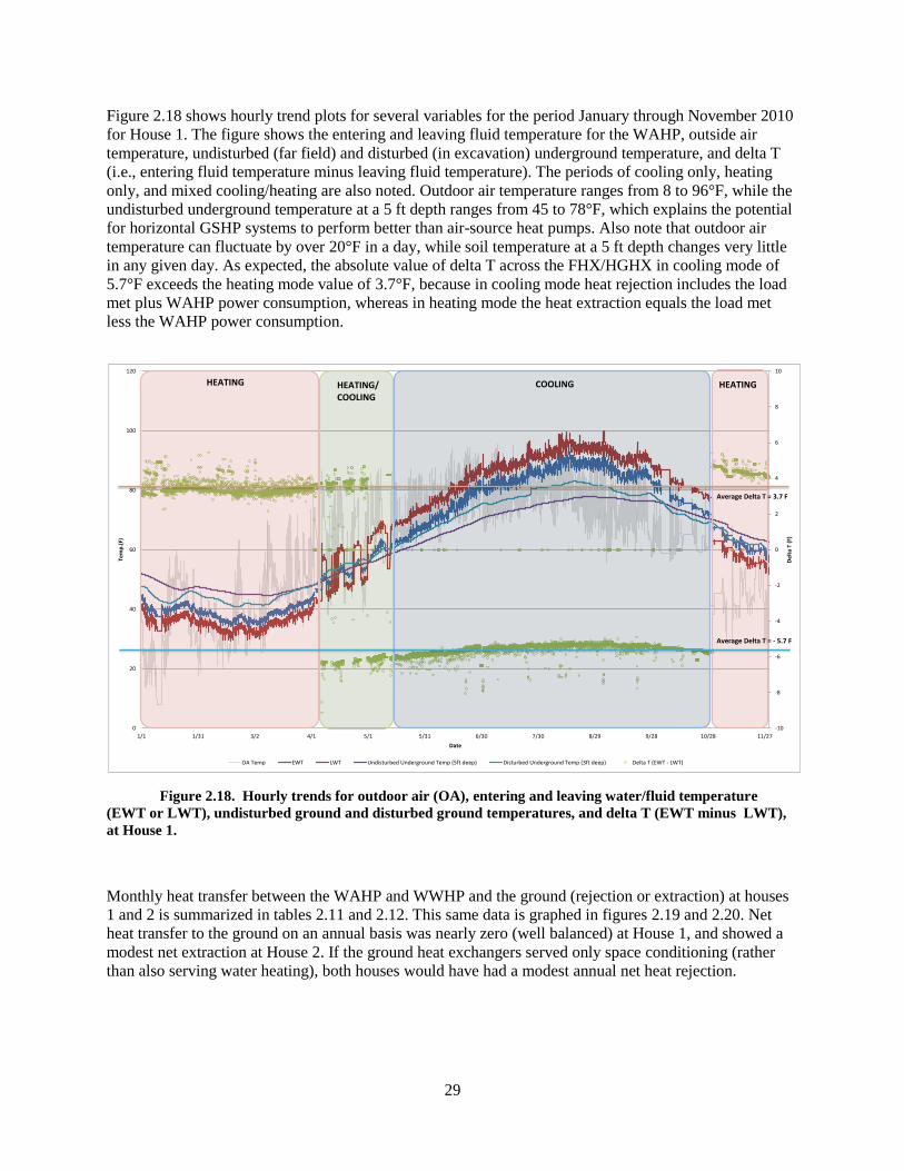
Figure 2.18 shows hourly trend plots for several variables for the period January through November 2010
for House 1. The figure shows the entering and leaving fluid temperature for the WAHP, outside air
temperature, undisturbed (far field) and disturbed (in excavation) underground temperature, and delta T
(i.e., entering fluid temperature minus leaving fluid temperature). The periods of cooling only, heating
only, and mixed cooling/heating are also noted. Outdoor air temperature ranges from 8 to 96°F, while the
undisturbed underground temperature at a 5 ft depth ranges from 45 to 78°F, which explains the potential
for horizontal GSHP systems to perform better than air-source heat pumps. Also note that outdoor air
temperature can fluctuate by over 20°F in a day, while soil temperature at a 5 ft depth changes very little
in any given day. As expected, the absolute value of delta T across the FHX/HGHX in cooling mode of
5.7°F exceeds the heating mode value of 3.7°F, because in cooling mode heat rejection includes the load
met plus WAHP power consumption, whereas in heating mode the heat extraction equals the load met
less the WAHP power consumption.
Figure 2.18. Hourly trends for outdoor air (OA), entering and leaving water/fluid temperature
(EWT or LWT), undisturbed ground and disturbed ground temperatures, and delta T (EWT minus LWT),
at House 1.
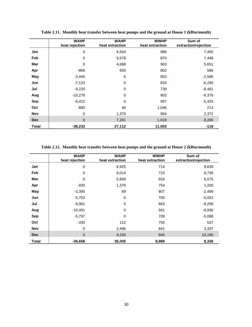
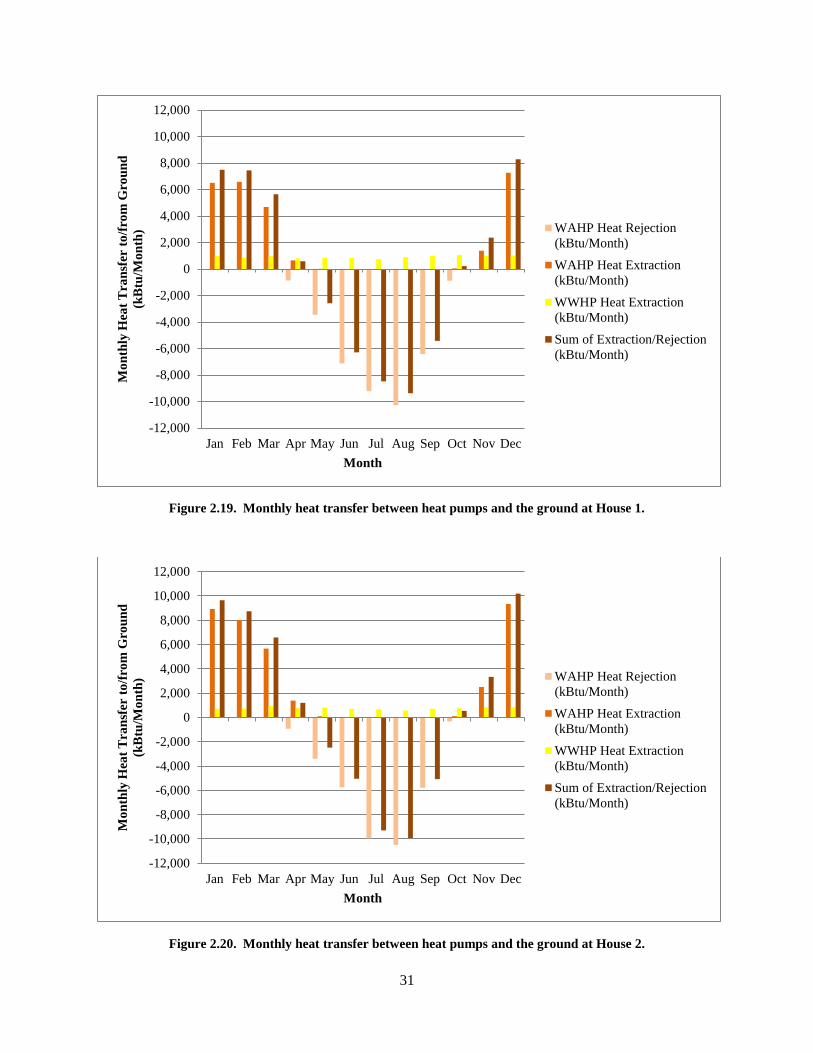
Monthly heat transfer between the WAHP and WWHP and the ground (rejection or extraction) at houses
1 and 2 is summarized in tables 2.11 and 2.12. This same data is graphed in figures 2.19 and 2.20. Net
heat transfer to the ground on an annual basis was nearly zero (well balanced) at House 1, and showed a
modest net extraction at House 2. If the ground heat exchangers served only space conditioning (rather
than also serving water heating), both houses would have had a modest annual net heat rejection.
-10
-8
-6
-4
-2
0
2
4
6
8
10
0
20
40
60
80
100
120
1/1 1/31 3/2 4/1 5/1 5/31 6/30 7/30 8/29 9/28 10/28 11/27
De
lta
T (F
)
Tem
p.(
F)
Date
OA Temp EWT LWT Undisturbed Underground Temp (5ft deep) Disturbed Underground Temp (3ft deep) Delta T (EWT - LWT)
Average Delta T = 3.7 F
Average Delta T = - 5.7 F
HEATING HEATINGCOOLINGHEATING/COOLING
30
Table 2.11. Monthly heat transfer between heat pumps and the ground at House 1 (kBtu/month)
WAHP
heat rejection WAHP
heat extraction WWHP
heat extraction Sum of
extraction/rejection
Jan 0 6,504 986 7,490
Feb 0 6,578 870 7,448
Mar 0 4,688 963 5,651
Apr -866 650 802 586
May -3,445 6 853 -2,586
Jun -7,123 0 833 -6,290
Jul -9,220 0 739 -8,481
Aug -10,278 0 902 -9,376
Sep -6,422 0 997 -5,425
Oct -880 46 1,046 213
Nov 0 1,379 994 2,372
Dec 0 7,261 1,019 8,280
Total -38,233 27,112 11,003 -118
Table 2.12. Monthly heat transfer between heat pumps and the ground at House 2 (kBtu/month)
WAHP heat rejection
WAHP heat extraction
WWHP heat extraction
Sum of extraction/rejection
Jan 0 8,925 714 9,639
Feb 0 8,014 723 8,736
Mar 0 5,658 916 6,575
Apr -930 1,376 754 1,200
May -3,395 89 807 -2,499
Jun -5,753 0 700 -5,052
Jul -9,961 0 663 -9,298
Aug -10,491 0 561 -9,930
Sep -5,797 0 709 -5,088
Oct -330 112 755 537
Nov 0 2,496 841 3,337
Dec 0 9,335 845 10,180
Total -36,658 36,005 8,989 8,336
31
Figure 2.19. Monthly heat transfer between heat pumps and the ground at House 1.
Figure 2.20. Monthly heat transfer between heat pumps and the ground at House 2.
-12,000
-10,000
-8,000
-6,000
-4,000
-2,000
0
2,000
4,000
6,000
8,000
10,000
12,000
Jan Feb Mar Apr May Jun Jul Aug Sep Oct Nov Dec
Mo
nth
ly H
eat
Tra
nsf
er t
o/f
rom
Gro
un
d
(kB
tu/M
on
th)
Month
WAHP Heat Rejection
(kBtu/Month)
WAHP Heat Extraction
(kBtu/Month)
WWHP Heat Extraction
(kBtu/Month)
Sum of Extraction/Rejection
(kBtu/Month)
32
3. NUMERICAL MODEL AND DESIGN TOOL DEVELOPMENT AND VALIDATION
3.1 Objectives and Approach
A key objective of this research project was to develop and validate the necessary energy performance
models and design tools so that GSHP systems using FHX (ground heat exchangers installed in the
overcut around basement walls) or hybrid FHX/HGHX (with some of the ground heat exchangers
installed in utility, footer drain, or supplemental trenches) can be designed and deployed with confidence
wherever they are feasible. The project focused on the greatest technical challenge, which was developing
and validating models and design tools for FHX. (Ground heat exchangers in utility and footer drain
trenches are essentially no different from HGHX in supplemental trenches, and models and design tools
for HGHX already exist.) This research project does not explicitly address ground heat exchangers
installed below the basement floor, which have very simple geometry and boundary conditions, and we
felt that this capability could be added to the models and design tools later. In fact, the computationally
efficient 3D model (described in Section 3.4) can model ground heat exchangers below the basement
floor.
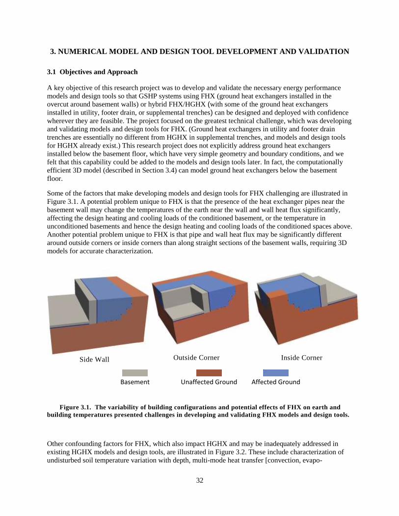
Some of the factors that make developing models and design tools for FHX challenging are illustrated in
Figure 3.1. A potential problem unique to FHX is that the presence of the heat exchanger pipes near the
basement wall may change the temperatures of the earth near the wall and wall heat flux significantly,
affecting the design heating and cooling loads of the conditioned basement, or the temperature in
unconditioned basements and hence the design heating and cooling loads of the conditioned spaces above.
Another potential problem unique to FHX is that pipe and wall heat flux may be significantly different
around outside corners or inside corners than along straight sections of the basement walls, requiring 3D
models for accurate characterization.
Side Wall
Outside Corner
Inside Corner
Figure 3.1. The variability of building configurations and potential effects of FHX on earth and
building temperatures presented challenges in developing and validating FHX models and design tools.
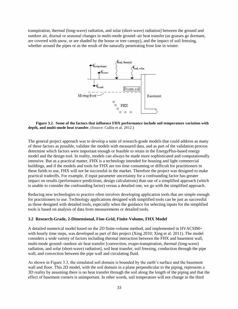
Other confounding factors for FHX, which also impact HGHX and may be inadequately addressed in
existing HGHX models and design tools, are illustrated in Figure 3.2. These include characterization of
undisturbed soil temperature variation with depth, multi-mode heat transfer [convection, evapo-
Basement Unaffected Ground Affected Ground
33
transpiration, thermal (long-wave) radiation, and solar (short-wave) radiation] between the ground and
outdoor air, diurnal or seasonal changes in multi-mode groundair heat transfer (as grasses go dormant,
are covered with snow, or are shaded by the house or tree canopy), and the impact of soil freezing,
whether around the pipes or as the result of the naturally penetrating frost line in winter.
Figure 3.2. Some of the factors that influence FHX performance include soil temperature variation with
depth, and multi-mode heat transfer. (Source: Cullin et al. 2012.)
The general project approach was to develop a suite of research-grade models that could address as many
of these factors as possible, validate the models with measured data, and as part of the validation process
determine which factors were important enough or feasible to retain in the EnergyPlus-based energy
model and the design tool. In reality, models can always be made more sophisticated and computationally
intensive. But as a practical matter, FHX is a technology intended for housing and light commercial
buildings, and if the models and tools for FHX are too time consuming or difficult for practitioners in
these fields to use, FHX will not be successful in the market. Therefore the project was designed to make
practical tradeoffs. For example, if input parameter uncertainty for a confounding factor has greater
impact on results (performance predictions, design calculations) than use of a simplified approach (which
is unable to consider the confounding factor) versus a detailed one, we go with the simplified approach.
Reducing new technologies to practice often involves developing application tools that are simple enough
for practitioners to use. Technology applications designed with simplified tools can be just as successful
as those designed with detailed tools, especially when the guidance for selecting inputs for the simplified
tools is based on analysis of data from measurements or detailed tools.
3.2 Research-Grade, 2-Dimensional, Fine-Grid, Finite-Volume, FHX Model
A detailed numerical model based on the 2D finite-volume method, and implemented in HVACSIM+
with hourly time steps, was developed as part of this project (Xing 2010; Xing et al. 2011). The model
considers a wide variety of factors including thermal interaction between the FHX and basement wall,
multi-mode groundoutdoor air heat transfer [convection, evapo-transpiration, thermal (long-wave)
radiation, and solar (short-wave) radiation], soil heat transfer, soil freezing, conduction through the pipe
wall, and convection between the pipe wall and circulating fluid.
As shown in Figure 3.3, the simulated soil domain is bounded by the earth’s surface and the basement
wall and floor. This 2D model, with the soil domain in a plane perpendicular to the piping, represents a
3D reality by assuming there is no heat transfer through the soil along the length of the piping and that the
effect of basement corners is unimportant. In other words, soil temperature will not change in the third
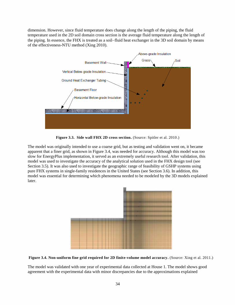
34
dimension. However, since fluid temperature does change along the length of the piping, the fluid
temperature used in the 2D soil domain cross section is the average fluid temperature along the length of
the piping. In essence, the FHX is treated as a soilfluid heat exchanger in the 3D soil domain by means
of the effectiveness-NTU method (Xing 2010).
Figure 3.3. Side wall FHX 2D cross section. (Source: Spitler et al. 2010.)
The model was originally intended to use a coarse grid, but as testing and validation went on, it became
apparent that a finer grid, as shown in Figure 3.4, was needed for accuracy. Although this model was too
slow for EnergyPlus implementation, it served as an extremely useful research tool. After validation, this
model was used to investigate the accuracy of the analytical solution used in the FHX design tool (see
Section 3.5). It was also used to investigate the geographic range of feasibility of GSHP systems using
pure FHX systems in single-family residences in the United States (see Section 3.6). In addition, this
model was essential for determining which phenomena needed to be modeled by the 3D models explained
later.
Figure 3.4. Non-uniform fine grid required for 2D finite-volume model accuracy. (Source: Xing et al. 2011.)
The model was validated with one year of experimental data collected at House 1. The model shows good
agreement with the experimental data with minor discrepancies due to the approximations explained
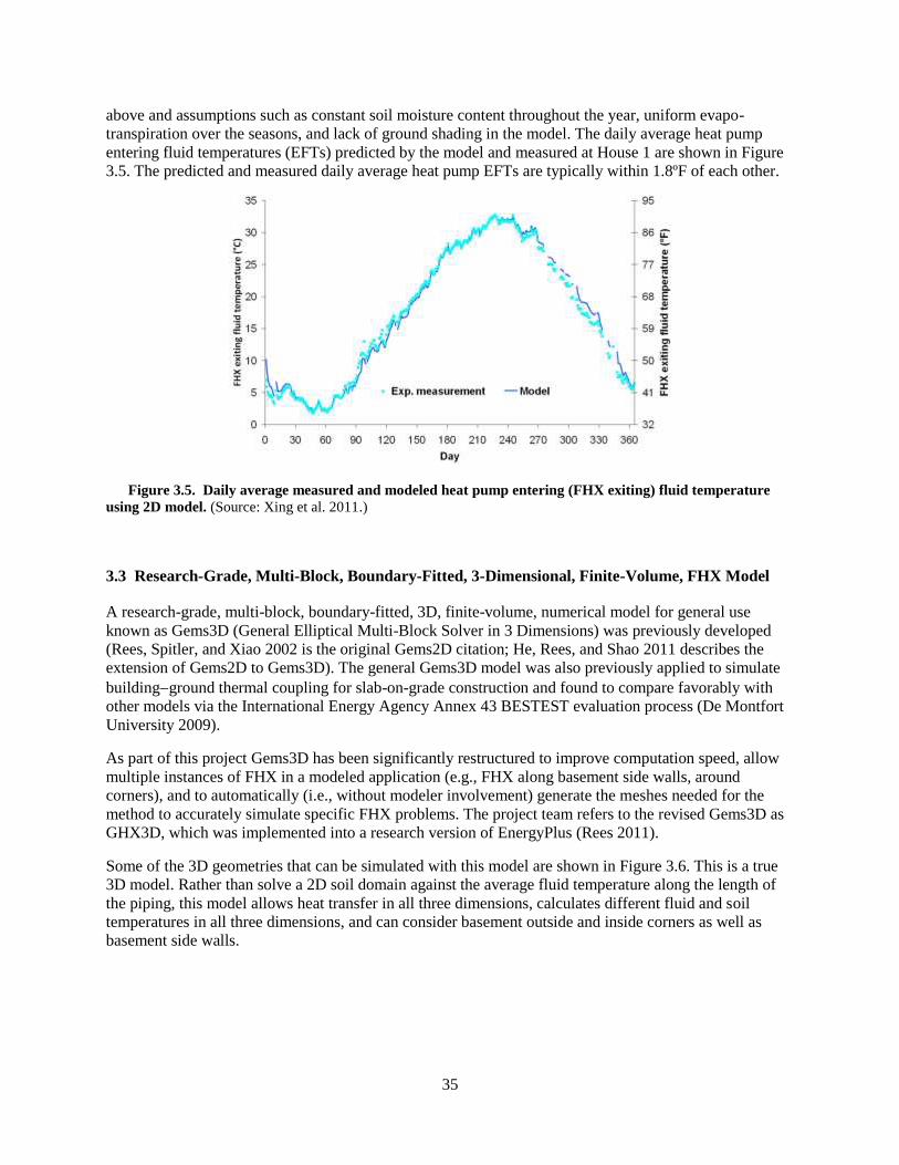
35
above and assumptions such as constant soil moisture content throughout the year, uniform evapo-
transpiration over the seasons, and lack of ground shading in the model. The daily average heat pump
entering fluid temperatures (EFTs) predicted by the model and measured at House 1 are shown in Figure
3.5. The predicted and measured daily average heat pump EFTs are typically within 1.8ºF of each other.
Figure 3.5. Daily average measured and modeled heat pump entering (FHX exiting) fluid temperature
using 2D model. (Source: Xing et al. 2011.)
3.3 Research-Grade, Multi-Block, Boundary-Fitted, 3-Dimensional, Finite-Volume, FHX Model
A research-grade, multi-block, boundary-fitted, 3D, finite-volume, numerical model for general use
known as Gems3D (General Elliptical Multi-Block Solver in 3 Dimensions) was previously developed
(Rees, Spitler, and Xiao 2002 is the original Gems2D citation; He, Rees, and Shao 2011 describes the
extension of Gems2D to Gems3D). The general Gems3D model was also previously applied to simulate
buildingground thermal coupling for slab-on-grade construction and found to compare favorably with
other models via the International Energy Agency Annex 43 BESTEST evaluation process (De Montfort
University 2009).
As part of this project Gems3D has been significantly restructured to improve computation speed, allow
multiple instances of FHX in a modeled application (e.g., FHX along basement side walls, around
corners), and to automatically (i.e., without modeler involvement) generate the meshes needed for the
method to accurately simulate specific FHX problems. The project team refers to the revised Gems3D as
GHX3D, which was implemented into a research version of EnergyPlus (Rees 2011).
Some of the 3D geometries that can be simulated with this model are shown in Figure 3.6. This is a true
3D model. Rather than solve a 2D soil domain against the average fluid temperature along the length of
the piping, this model allows heat transfer in all three dimensions, calculates different fluid and soil
temperatures in all three dimensions, and can consider basement outside and inside corners as well as
basement side walls.
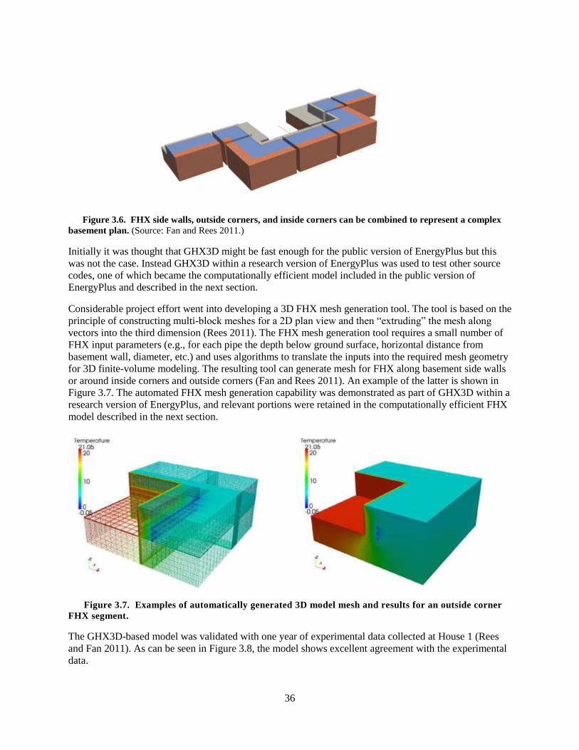
36
Figure 3.6. FHX side walls, outside corners, and inside corners can be combined to represent a complex
basement plan. (Source: Fan and Rees 2011.)
Initially it was thought that GHX3D might be fast enough for the public version of EnergyPlus but this
was not the case. Instead GHX3D within a research version of EnergyPlus was used to test other source
codes, one of which became the computationally efficient model included in the public version of
EnergyPlus and described in the next section.
Considerable project effort went into developing a 3D FHX mesh generation tool. The tool is based on the
principle of constructing multi-block meshes for a 2D plan view and then “extruding” the mesh along
vectors into the third dimension (Rees 2011). The FHX mesh generation tool requires a small number of
FHX input parameters (e.g., for each pipe the depth below ground surface, horizontal distance from
basement wall, diameter, etc.) and uses algorithms to translate the inputs into the required mesh geometry
for 3D finite-volume modeling. The resulting tool can generate mesh for FHX along basement side walls
or around inside corners and outside corners (Fan and Rees 2011). An example of the latter is shown in
Figure 3.7. The automated FHX mesh generation capability was demonstrated as part of GHX3D within a
research version of EnergyPlus, and relevant portions were retained in the computationally efficient FHX
model described in the next section.
Figure 3.7. Examples of automatically generated 3D model mesh and results for an outside corner
FHX segment.
The GHX3D-based model was validated with one year of experimental data collected at House 1 (Rees
and Fan 2011). As can be seen in Figure 3.8, the model shows excellent agreement with the experimental
data.
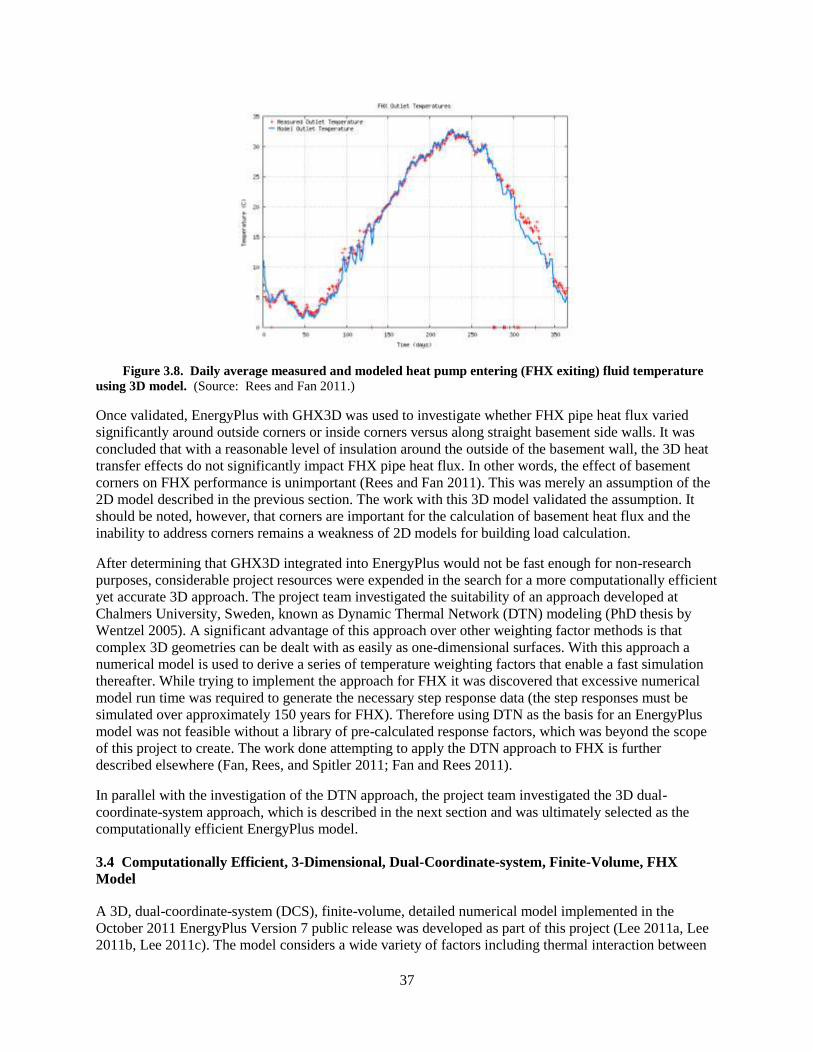
37
Figure 3.8. Daily average measured and modeled heat pump entering (FHX exiting) fluid temperature
using 3D model. (Source: Rees and Fan 2011.)
Once validated, EnergyPlus with GHX3D was used to investigate whether FHX pipe heat flux varied
significantly around outside corners or inside corners versus along straight basement side walls. It was
concluded that with a reasonable level of insulation around the outside of the basement wall, the 3D heat
transfer effects do not significantly impact FHX pipe heat flux. In other words, the effect of basement
corners on FHX performance is unimportant (Rees and Fan 2011). This was merely an assumption of the
2D model described in the previous section. The work with this 3D model validated the assumption. It
should be noted, however, that corners are important for the calculation of basement heat flux and the
inability to address corners remains a weakness of 2D models for building load calculation.
After determining that GHX3D integrated into EnergyPlus would not be fast enough for non-research
purposes, considerable project resources were expended in the search for a more computationally efficient
yet accurate 3D approach. The project team investigated the suitability of an approach developed at
Chalmers University, Sweden, known as Dynamic Thermal Network (DTN) modeling (PhD thesis by
Wentzel 2005). A significant advantage of this approach over other weighting factor methods is that
complex 3D geometries can be dealt with as easily as one-dimensional surfaces. With this approach a
numerical model is used to derive a series of temperature weighting factors that enable a fast simulation
thereafter. While trying to implement the approach for FHX it was discovered that excessive numerical
model run time was required to generate the necessary step response data (the step responses must be
simulated over approximately 150 years for FHX). Therefore using DTN as the basis for an EnergyPlus
model was not feasible without a library of pre-calculated response factors, which was beyond the scope
of this project to create. The work done attempting to apply the DTN approach to FHX is further
described elsewhere (Fan, Rees, and Spitler 2011; Fan and Rees 2011).
In parallel with the investigation of the DTN approach, the project team investigated the 3D dual-
coordinate-system approach, which is described in the next section and was ultimately selected as the
computationally efficient EnergyPlus model.
3.4 Computationally Efficient, 3-Dimensional, Dual-Coordinate-system, Finite-Volume, FHX
Model
A 3D, dual-coordinate-system (DCS), finite-volume, detailed numerical model implemented in the
October 2011 EnergyPlus Version 7 public release was developed as part of this project (Lee 2011a, Lee
2011b, Lee 2011c). The model considers a wide variety of factors including thermal interaction between
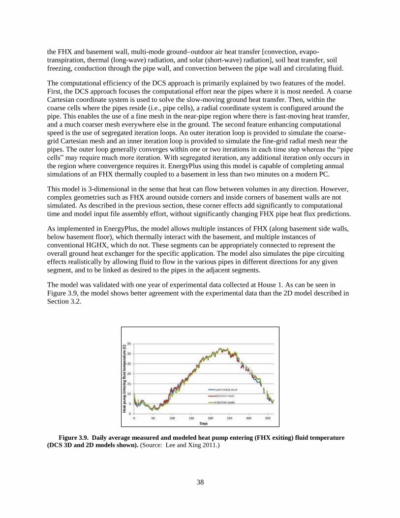
38
the FHX and basement wall, multi-mode groundoutdoor air heat transfer [convection, evapo-
transpiration, thermal (long-wave) radiation, and solar (short-wave) radiation], soil heat transfer, soil
freezing, conduction through the pipe wall, and convection between the pipe wall and circulating fluid.
The computational efficiency of the DCS approach is primarily explained by two features of the model.
First, the DCS approach focuses the computational effort near the pipes where it is most needed. A coarse
Cartesian coordinate system is used to solve the slow-moving ground heat transfer. Then, within the
coarse cells where the pipes reside (i.e., pipe cells), a radial coordinate system is configured around the
pipe. This enables the use of a fine mesh in the near-pipe region where there is fast-moving heat transfer,
and a much coarser mesh everywhere else in the ground. The second feature enhancing computational
speed is the use of segregated iteration loops. An outer iteration loop is provided to simulate the coarse-
grid Cartesian mesh and an inner iteration loop is provided to simulate the fine-grid radial mesh near the
pipes. The outer loop generally converges within one or two iterations in each time step whereas the “pipe
cells” may require much more iteration. With segregated iteration, any additional iteration only occurs in
the region where convergence requires it. EnergyPlus using this model is capable of completing annual
simulations of an FHX thermally coupled to a basement in less than two minutes on a modern PC.
This model is 3-dimensional in the sense that heat can flow between volumes in any direction. However,
complex geometries such as FHX around outside corners and inside corners of basement walls are not
simulated. As described in the previous section, these corner effects add significantly to computational
time and model input file assembly effort, without significantly changing FHX pipe heat flux predictions.
As implemented in EnergyPlus, the model allows multiple instances of FHX (along basement side walls,
below basement floor), which thermally interact with the basement, and multiple instances of
conventional HGHX, which do not. These segments can be appropriately connected to represent the
overall ground heat exchanger for the specific application. The model also simulates the pipe circuiting
effects realistically by allowing fluid to flow in the various pipes in different directions for any given
segment, and to be linked as desired to the pipes in the adjacent segments.
The model was validated with one year of experimental data collected at House 1. As can be seen in
Figure 3.9, the model shows better agreement with the experimental data than the 2D model described in
Section 3.2.
Figure 3.9. Daily average measured and modeled heat pump entering (FHX exiting) fluid temperature
(DCS 3D and 2D models shown). (Source: Lee and Xing 2011.)
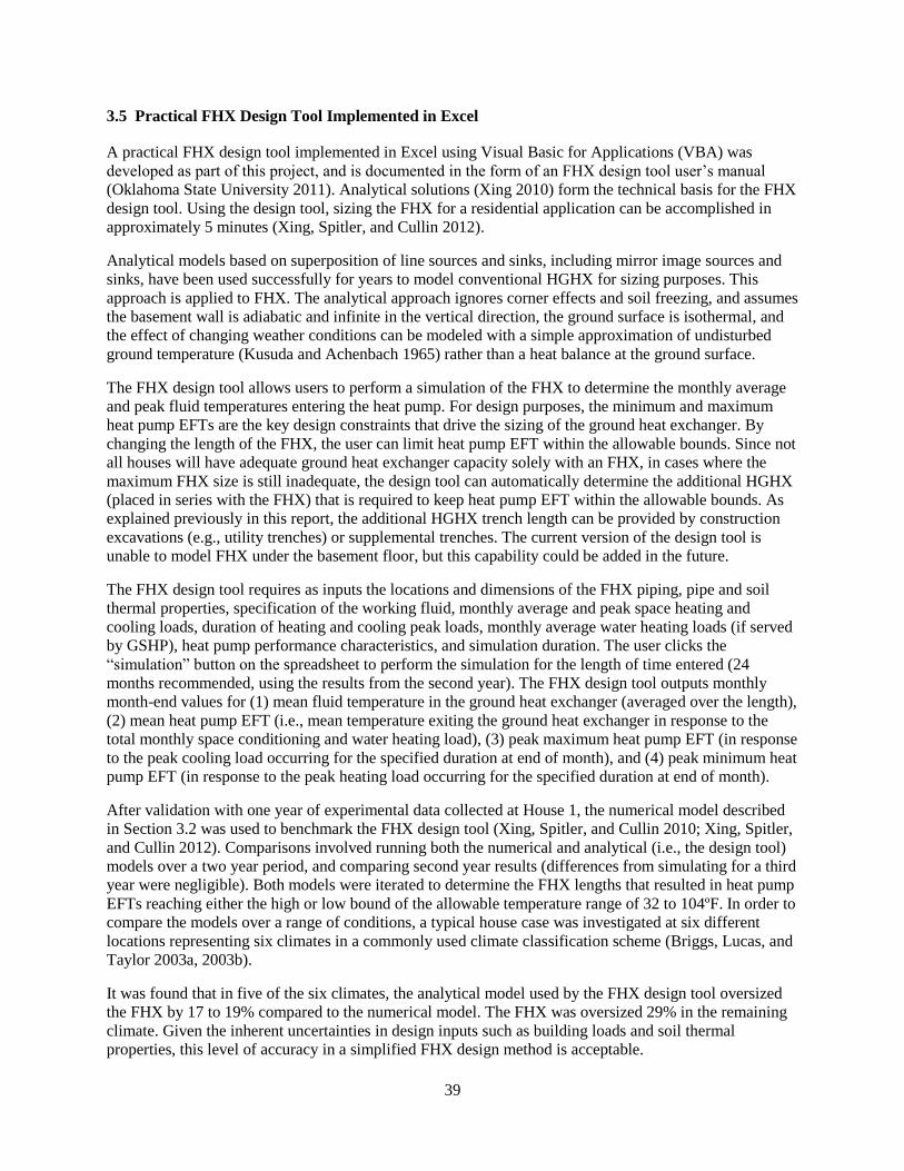
39
3.5 Practical FHX Design Tool Implemented in Excel
A practical FHX design tool implemented in Excel using Visual Basic for Applications (VBA) was
developed as part of this project, and is documented in the form of an FHX design tool user’s manual
(Oklahoma State University 2011). Analytical solutions (Xing 2010) form the technical basis for the FHX
design tool. Using the design tool, sizing the FHX for a residential application can be accomplished in
approximately 5 minutes (Xing, Spitler, and Cullin 2012).
Analytical models based on superposition of line sources and sinks, including mirror image sources and
sinks, have been used successfully for years to model conventional HGHX for sizing purposes. This
approach is applied to FHX. The analytical approach ignores corner effects and soil freezing, and assumes
the basement wall is adiabatic and infinite in the vertical direction, the ground surface is isothermal, and
the effect of changing weather conditions can be modeled with a simple approximation of undisturbed
ground temperature (Kusuda and Achenbach 1965) rather than a heat balance at the ground surface.
The FHX design tool allows users to perform a simulation of the FHX to determine the monthly average
and peak fluid temperatures entering the heat pump. For design purposes, the minimum and maximum
heat pump EFTs are the key design constraints that drive the sizing of the ground heat exchanger. By
changing the length of the FHX, the user can limit heat pump EFT within the allowable bounds. Since not
all houses will have adequate ground heat exchanger capacity solely with an FHX, in cases where the
maximum FHX size is still inadequate, the design tool can automatically determine the additional HGHX
(placed in series with the FHX) that is required to keep heat pump EFT within the allowable bounds. As
explained previously in this report, the additional HGHX trench length can be provided by construction
excavations (e.g., utility trenches) or supplemental trenches. The current version of the design tool is
unable to model FHX under the basement floor, but this capability could be added in the future.
The FHX design tool requires as inputs the locations and dimensions of the FHX piping, pipe and soil
thermal properties, specification of the working fluid, monthly average and peak space heating and
cooling loads, duration of heating and cooling peak loads, monthly average water heating loads (if served
by GSHP), heat pump performance characteristics, and simulation duration. The user clicks the
“simulation” button on the spreadsheet to perform the simulation for the length of time entered (24
months recommended, using the results from the second year). The FHX design tool outputs monthly
month-end values for (1) mean fluid temperature in the ground heat exchanger (averaged over the length),
(2) mean heat pump EFT (i.e., mean temperature exiting the ground heat exchanger in response to the
total monthly space conditioning and water heating load), (3) peak maximum heat pump EFT (in response
to the peak cooling load occurring for the specified duration at end of month), and (4) peak minimum heat
pump EFT (in response to the peak heating load occurring for the specified duration at end of month).
After validation with one year of experimental data collected at House 1, the numerical model described
in Section 3.2 was used to benchmark the FHX design tool (Xing, Spitler, and Cullin 2010; Xing, Spitler,
and Cullin 2012). Comparisons involved running both the numerical and analytical (i.e., the design tool)
models over a two year period, and comparing second year results (differences from simulating for a third
year were negligible). Both models were iterated to determine the FHX lengths that resulted in heat pump
EFTs reaching either the high or low bound of the allowable temperature range of 32 to 104ºF. In order to
compare the models over a range of conditions, a typical house case was investigated at six different
locations representing six climates in a commonly used climate classification scheme (Briggs, Lucas, and
Taylor 2003a, 2003b).
It was found that in five of the six climates, the analytical model used by the FHX design tool oversized
the FHX by 17 to 19% compared to the numerical model. The FHX was oversized 29% in the remaining
climate. Given the inherent uncertainties in design inputs such as building loads and soil thermal
properties, this level of accuracy in a simplified FHX design method is acceptable.
40
As a further validation of the design tool, the “as-built” design values from House 1 were used to generate
the inputs required for the design tool analysis. The input parameters describing the hybrid FHX/HGHX
application at House 1 are summarized in Table 3.1. As described in Section 2.4, the averages of pipe
depth and pipe distance from the basement wall over the 100 ft FHX excavation, for each of the six pipes,
were generated using the 3D CAD model. Other inputs required by the design tool, such the heat pump
performance data, monthly cooling and heating loads, and domestic water heating loads, are documented
previously in this report. With these inputs, the design tool estimated maximum and minimum EFTs of
96°F and 29°F, respectively. By varying HGHX excavation length and re-running the design tool, it was
estimated that the total House 1 excavation length would have to be increased from 300 ft to 369 ft in
order for the design tool to output the measured maximum and minimum EFTs. In other words, the design
tool calculation oversized the hybrid FHX/HGHX excavation length by 23% compared to the House 1
experiment, which is consistent with the findings relative to the numerical model described above.
Table 3.1. Design tool input parameters for the as-is FHX/HGHX at House 1
System and foundation heat exchanger (FHX) input parameters
Thermal conductivity of the soil 0.70 Btu/(hr-ft-°F)
Specific heat of the soil 0.25 Btu/lb-°F
Density of the soil 120.0 lb/ft3
Undisturbed ground temperature 61.0 °F
Surface amplitude 22.0 °F
Volumetric flow rate 6.0 Gal/min
Working fluid Propylene glycol ---
Concentration of working fluid 20 % by wt
Number of pipes 6 ---
Length of FHX excavation 100.0 ft
Pipe inside diameter 0.86 in
Pipe outside diameter 1.05 in
Pipe thermal conductivity 0.23 Btu/(hr-ft-°F)
Number of months to run 36 months
Additional horizontal ground heat exchanger (HGHX) input parameters
Number of pipes 6 --
Length of HGHX excavation 200.0 ft
FHX pipe number
FHX depth below ground
(ft)
FHX distance from basement wall (ft)
Pipe 1 7.3 1.7
Pipe 2 7.4 2.5
Pipe 3 7.1 3.3
Pipe 4 6.4 3.6
Pipe 5 5.5 3.7
Pipe 6 4.6 3.6
HGHX pipe number
HGHX depth below ground
(ft)
HGHX distance between Pipe 1
and Pipe N (ft)
Pipe 1 6.0 0.0
Pipe 2 6.0 1.3
Pipe 3 5.0 1
Pipe 4 5.0 1.6
Pipe 5 4.0 2
Pipe 6 4.0 2.3
41
3.6 Geographic Range of Feasibility of GSHP Systems Using FHX in the United States
ORNL had previously demonstrated that an FHX-based GSHP system was feasible for a specific small
ultra-high-energy-efficiency house in one climate (Christian and Bonar 2008). In order to investigate the
geographic range of feasibility of GSHP systems using FHX in single-family residences in the United
States, a small-scale parametric study was performed as part of this project (Cullin et al. 2012).
A one-story house over a full basement with characteristics similar to the original ORNL demonstration
house was used as the basis of the study. Two house cases, “high insulation (HI)” and “very high
insulation (VHI),” were studied in 17 locations. In all locations the houses were assumed to be on flat
terrain, have full basements, and have an FHX that encircles the entire perimeter of the house. In this
preliminary study, EnergyPlus was used to generate the space conditioning load for the one-story house,
and HVACSIM+ was used to generate the space conditioning load for the basement space and for
simulation of the HVAC and FHX systems. The 2D, finite-volume, numerical model described in Section
3.2 and implemented in HVACSIM+ was used to simulate the FHX (Xing 2010). An iterative technique
was used between EnergyPlus and HVACSIM+ so that the total house load (house and basement)
successfully converged in each time step.
Hourly simulations were run for each combination of location and insulation level. For cases in which the
heat pump EFT deviated above or below the allowable design limits, a 100 ft supplemental horizontal
ground heat exchanger was added to the FHX in series and another simulation performed. The EFT
design limits for this study were 30.2°F for heating and 99.5°F for cooling, with a working fluid of 10%
propylene glycol by weight in water.
From among the 34 cases, there were four cases (Billings HI, Chicago HI, Minneapolis HI, Minneapolis
VHI) where EFT deviated below the minimum constraint, and four cases (Houston HI, Phoenix HI,
Phoenix VHI, Tallahassee HI) where EFT deviated above the maximum constraint. After adding a 100 ft
supplemental horizontal ground heat exchanger, seven or the eight cases had EFT within allowable
design limits, leaving only one case (Minneapolis HI) where EFT deviated below the minimum
constraint.
This preliminary analysis was used to construct Figure 3.10, which is a map of the United States showing
where GSHP systems using FHX in single-family residences appear to be feasible. There are three zones
of feasibility: not recommended, marginal, and feasible. Since the high-insulation cases represent current
recommended best practice, those results were used to construct the map. A map using the VHI results
would show even greater geographic feasibility. The “not recommended” zone indicates locations (such
as Minneapolis) where FHX cannot be expected to work, even with the addition of a 100 ft supplemental
HGHX. The “marginal” zone includes locations that might require a supplemental HGHX (such as
Billings and Houston), as well as locations where the heat pump EFTs may be fairly close to the
constraints, say,within two degrees Fahrenheit or so. Finally, the “feasible” area contains the locations
where FHX may be expected to work without supplement from an HGHX.
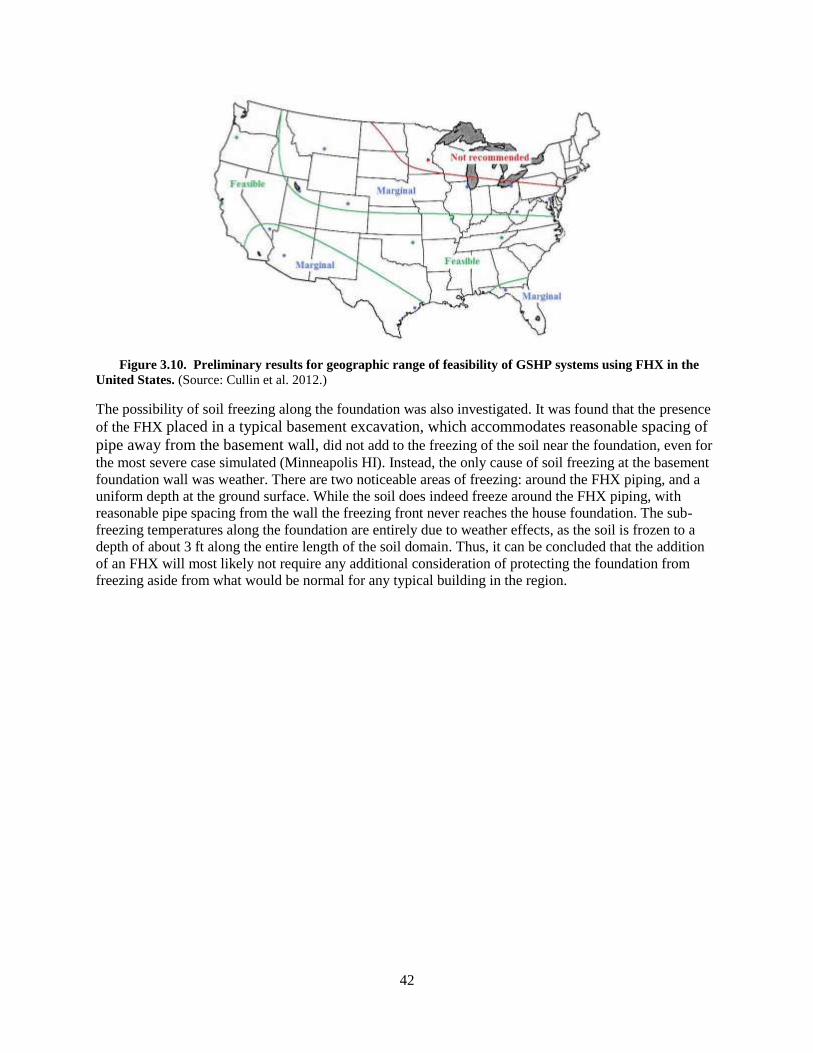
42
Figure 3.10. Preliminary results for geographic range of feasibility of GSHP systems using FHX in the
United States. (Source: Cullin et al. 2012.)
The possibility of soil freezing along the foundation was also investigated. It was found that the presence
of the FHX placed in a typical basement excavation, which accommodates reasonable spacing of
pipe away from the basement wall, did not add to the freezing of the soil near the foundation, even for
the most severe case simulated (Minneapolis HI). Instead, the only cause of soil freezing at the basement
foundation wall was weather. There are two noticeable areas of freezing: around the FHX piping, and a
uniform depth at the ground surface. While the soil does indeed freeze around the FHX piping, with
reasonable pipe spacing from the wall the freezing front never reaches the house foundation. The sub-
freezing temperatures along the foundation are entirely due to weather effects, as the soil is frozen to a
depth of about 3 ft along the entire length of the soil domain. Thus, it can be concluded that the addition
of an FHX will most likely not require any additional consideration of protecting the foundation from
freezing aside from what would be normal for any typical building in the region.
43
4. DISCUSSION
Conventional equipment for controlling the temperature and humidity of a building, or supplying hot
water and fresh outdoor air, must exchange energy (or heat) with the building’s outdoor environment.
Equipment using the ground as a heat source and heat sink consumes less non-renewable energy
(electricity and fossil fuels) because the earth is cooler than outdoor air in summer and warmer in winter.
The most important barrier to rapid growth of the GSHP industry is high first cost of GSHP systems to
consumers (Hughes 2008).
The most common GSHP system utilizes a closed-loop ground heat exchanger. This type of GSHP
system can be used almost anywhere. There is reason to believe that reducing the cost of closed-loop
systems is the best strategy for maximizing energy savings achieved with GSHP technology. The cost
premium of closed-loop GSHP systems over conventional space conditioning and water heating systems
is primarily associated with drilling boreholes or excavating trenches, installing vertical or horizontal
ground heat exchangers, and backfilling excavations.
This project investigates reducing the cost of horizontal closed-loop ground heat exchangers through the
use of construction excavations augmented when necessary with supplemental trenches. This approach
applies only to new construction of residential and light commercial buildings or additions to such
buildings. In general, construction excavations may include the overcut around the basement walls, below
the basement floor, utility trenches (for buried water, sewer and power), and trenches for draining the
foundation footers. In the business-as-usual scenario these construction excavations are not used for the
horizontal ground heat exchanger (HGHX); instead the HGHX is installed entirely in trenches dug
specifically for that purpose. The potential cost savings comes from using the construction excavations
for the installation of ground heat exchangers to the extent possible and thereby reducing the length of
trench that must be dug and backfilled. When construction excavations are used for double duty, adequate
spacing between the HGHX and utility pipes is of course required, but simple guidance on this issue is
expected to suffice.
The term foundation heat exchanger (FHX) has been coined to refer exclusively to ground heat exchanger
installed in the overcut around basement walls. The primary technical challenge in this project was the
development and validation of energy performance models and design tools for FHX. In terms of
performance modeling and design, ground heat exchangers in utility and footer drain trenches are no
different than conventional HGHX in conventional trenches, and models and design tools for HGHX
already exist.
Ground heat exchangers installed below the basement floor were not addressed. Project resources were
insufficient to address both FHX and sub-floor systems, and it was important to tackle the greatest
technical challenge first. Since the sub-floor case has very simple geometry and boundary conditions, the
project team felt confident that this capability could be added to the models and design tools later. As it
turned out, the computationally efficient performance model developed by this project is able to model
sub-floor systems, though this capability has not yet been validated against measured data.
This project developed and validated energy performance models and design tools so that FHX or hybrid
FHX/HGHX systems can be engineered with confidence, enabling this technology to be applied in
residential and light commercial buildings. The energy performance models developed and validated here
also address and solve another problem, the longstanding inadequacy in the way ground–building thermal
interaction is represented in building energy models, whether or not there is a ground heat exchanger
nearby.
44
Two side-by-side, three-level, unoccupied research houses with walkout basements, identical 3,700 ft2
floor plans, and hybrid FHX/HGHX systems were constructed to provide validation data sets for the
energy performance models and design tools for hybrid FHX/HGHX systems developed as part of the
project. In these unoccupied research houses, human impact on energy use is simulated to match the
national average, with showers, lights, ovens, washers, and other energy-consuming equipment turned on
and off at exactly the same times. The ground heat exchangers in the two houses were intentionally
similar to provide experimental redundancy, essentially guaranteeing that experimental data would be
available. Validation was based on the House 1 data set primarily because the sizing of the hybrid
FHX/HGHX system there (done without an FHX design tool) turned out to be closer to what was needed
than at House 2.
The envelopes of both houses are very energy efficient and airtight, with HERS ratings of 44 and 45
respectively. Both houses are mechanically ventilated with energy recovery ventilators with space
conditioning provided by WAHPs with 2 ton nominal capacities. For comparison, typically in East
Tennessee, a house built to code and having 3,700 ft2 of floor space would require a 4 to 5 ton nominal
capacity unit for space conditioning. Separate WWHPs with 1.5 ton nominal capacities were used for
water heating. Hot water usage is simulated to match the national average (54 gallons per day) for houses
of this size and having these characteristics. The WAHP and WWHP units are connected to the ground
heat exchanger in parallel with each other.
At House 1 the total excavation length for the hybrid FHX/HGHX system is 300 ft, including 100 ft of
FHX in the overcut around basement walls, 80 ft in utility trenches, and 120 ft in supplemental trenches.
Hence 60% of the excavations used for installation of the ground heat exchanger (180 of 300 ft) were
required anyway to construct the home. At House 2 the total excavation is 360 ft and there is 100 ft of
FHX in the overcut around basement walls, 80 ft in utility trenches, and 180 ft in supplemental trenches,
so 50% is in construction excavations. There are six pipes in all excavations, meaning three parallel
circuits taking the working fluid out and back. All circuit pipes are ¾ inch nominal diameter high density
polyethylene. The multiple instances of FHX in basement wall overcuts and HGHX in utility or
supplemental trenches are all connected in series. The working fluid is 20% by weight propylene glycol in
water.
Data was collected at both houses and stored using Campbell Scientific Model CR3000 micro-loggers
and retrieved remotely over dedicated telephone lines during January through November 2010. In general
the data is measured at a rapid scan rate with averages logged at 15 minute intervals, but some channels
were logged at intervals as short as 1 minute, as necessary. Measured equipment performance at houses 1
and 2 included WAHP heating season COPs of 3.6 and 3.6, WAHP cooling season COPs of 4.2 and 4.1,
and WWHP annual COPs of 3.1 and 2.6. Annual maximum and minimum heat pump EFTs measured at
houses 1 and 2 were 93.2°F and 33.4°F, and 90.3°F and 33.7°F, respectively. The full 15 minute interval
data set from House 1 was used to validate the energy performance models and design tool.
Model and design tool development proceeded in parallel with construction, installing instrumentation,
and monitoring the houses for a year. Several detailed numerical models for FHX were developed as part
of the project. Essentially the project team was searching for an energy performance model accurate
enough to achieve project objectives while also having sufficient computational efficiency for practical
use in EnergyPlus. A 3D, dual-coordinate-system (DCS), finite-volume model satisfied these criteria and
was included in the October 2011 EnergyPlus Version 7 public release after being validated against the
measured data. EnergyPlus using this model is capable of completing annual simulations of an FHX
thermally coupled to a basement in less than two minutes on a modern PC. As an extra bonus, the DCS
model can simulate FHX installed below the basement floor, but this capability has not been validated
with measured data.
45
A practical design tool for sizing pure FHX or hybrid FHX/HGHX systems was also developed and
implemented in Excel using Visual Basic for Applications. Using the design tool, sizing the FHX or
FHX/HGHX for a residential application can be accomplished in approximately 5 minutes. Compared to
one of the numerical models, the design tool was found to oversize the ground heat exchanger by 17 to
20% in five of six benchmarking locations, and by 29% in the remaining location. The design tool
oversized the hybrid FHX/HGHX system at House 1 by 23%. Given the inherent uncertainties in design
inputs such as building loads and soil thermal properties, this level of accuracy in a simplified FHX
design method is acceptable.
One of the numerical models was used to investigate the geographic range of technical feasibility of FHX
systems. For a small well-insulated home with 1,600 sf on the first floor, a full basement beneath, and on
level terrain, with FHX on all four basement walls, the preliminary analysis indicated that pure FHX
systems were technically feasible for new construction in nearly half the United States. Although not
investigated, hybrid FHX/HGHX systems should have some level of installed cost savings over
conventional HGHX systems in almost any residential or light commercial new construction project
involving significant excavation.
Preliminary estimates indicate that when implemented at scale by a production builder, ground heat
exchanger in construction excavations (FHX in overcut around basement or HGHX in utility trenches)
may be feasible at $1,000 per ton. That compares with traditional vertical-loop and six-pipe-per-virgin-
trench HGHX systems that typically are installed in East Tennessee at $3,000 per ton and $2,250 per ton,
respectively. If these values are correct, hybrid systems would warrant consideration even when use of
construction excavations exclusively is not feasible. For example, a 3-ton hybrid FHX/HGHX ground
heat exchanger application where construction excavations are adequate for two-thirds of the load would
cost $4,250 (2 x $1000 + $2,250) compared to $6,750 (3 x $2,250) for pure HGHX in virgin trench. The
actual cost of a particular project may vary depending on drilling/trenching conditions, regional cost
variations, underground soil thermal properties and building geometry. Whether cost reductions through
use of construction excavations are enough for GSHP systems to gain significantly broader consideration
in new construction markets remains to be seen.
In summary, the project has successfully developed and validated performance models and design tools
so that FHX or hybrid FHX/HGHX systems can be engineered with confidence, thus enabling the use of
construction excavations for ground heat exchangers to be applied on a large scale. Although it is
reasonable to assume that significant cost savings should be achievable from reducing supplemental
trench length by using construction excavations, this has yet to be proven. Toward that end, the authors
recommend the following next steps:
1. Production-basis approaches to implementing FHX or hybrid FHX/HGHX systems should be
developed. The materials, products, tools, and installation techniques used for this two-house
demonstration leave considerable room for improvement. Better approaches that are fast and
foolproof in the hands of site laborers must be invented (e.g., spray a layer of grout onto the trench
side walls using a new device akin to those for spraying or blowing insulations; lay prefabricated
mats of cross-linked, parallel, reduced-diameter HDPE tubes onto the grout; spray another layer of
grout; let the grout set; finish backfill with bulldozer, etc.).
2. Production-basis implementations of FHX or hybrid FHX/HGHX systems should be evaluated in a
variety of climates and soil conditions to further validate performance, determine cost, and develop
and document the installation standards for double-duty excavations. These projects should include in
their scope the field experiments and effort required to add validated capabilities for sub-basement-
floor FHX to the EnergyPlus model and Excel-based design tool developed here.

46
3. Documentation of any newly developed materials, products, tools, and installation standards should
flow into the appropriate industry tomes (e.g., IGSHPA installation manual, ASHRAE HVAC
Applications Handbook Chapter 34) to facilitate widespread use.
47
5. REFERENCES
ASHRAE (American Society of Heating, Refrigeration, and Air Conditioning Professionals). 2011.
ASHRAE Handbook of HVAC Applications, chapter 34, table 35, p34.15.
Boudreaux, P.R., and Anthony Gehl. 2011. Wolf Creek Appliance Control and Occupancy Simulation.
TVA Milestone Report D 6.1. Oak Ridge National Laboratory.
Briggs, R.S., R.G. Lucas, and T. Taylor. 2003a. Climate Classification for Building Energy Codes and
Standards: Part 1 - Development Process, Technical and Symposium Papers, ASHRAE Winter
Meeting, Chicago, IL, January, 2003.
Briggs, R.S., R.G. Lucas, and T. Taylor. 2003b. Climate Classification for Building Energy Codes and
Standards: Part 2 - Zone Definitions, Maps and Comparisons, Technical and Symposium Papers,
ASHRAE Winter Meeting, Chicago, IL, January, 2003.
Christian, J., and J. Bonar. 2008. Building a 40% Energy Saving House in the Mixed-Humid Climate,
ORNL/TM-2008/08, Oak Ridge National Laboratory, Oak Ridge, Tenn.
Code of Federal Regulations. 2010a. Uniform Test Method for Measuring the Energy Consumption of
Automatic and Semi-Automatic Clothes Washers. Title 10 part 430, Subpt B, Appendix J1.
http://ecfr.gpoaccess.gov/cgi/t/text/textidx?c=ecfr&sid=6de07a43f47ca869f23b5d2e416ff012&rgn=di
v9&view=text&node=10:3.0.1.4.16.2.9.6.11&idno=10.
Code of Federal Regulations. 2010b. Uniform Test Method for Measuring the Energy Consumption of
Electric Refrigerators and Electric Refrigerator-Freezers, Title 10 part 430, Subpt B, Appendix A1.
http://ecfr.gpoaccess.gov/cgi/t/text/textidx?c=ecfr&sid=6de07a43f47ca869f23b5d2e416ff012&rgn=di
v9&view=text&node=10:3.0.1.4.16.2.9.6.1&idno=10.
Cullin, J.R., L. Xing, E. Lee, J.D. Spitler, and D.E. Fisher. 2012. “Feasibility of Foundation Heat
Exchangers In Ground Source Heat Pump Systems in the United States.” ASHRAE Transactions:
submitted for review.
De Montfort University. 2009. Modeler Report for BESTEST Cases GC10a-GC80c Gems3D Version
2.07. Leicester, UK, De Montfort University. http://www.ornl.gov/sci/ees/etsd/btric/ground-
source.shtml.
Fan, D., and S.J. Rees. 2011. Three-Dimensional Mesh Generation Tools. Leicester, UK, DeMontfort
University. http://www.ornl.gov/sci/ees/etsd/btric/ground-source.shtml.
Fan, D., S.J. Rees, and J.D. Spitler. 2011. Application of Dynamic Thermal Networks to the Modeling of
Foundation Heat Exchangers. Building Simulation 2011. Sydney, Australia, IBPSA.
Fantech 2010. Fantech Energy Recovery Ventilator SER Series (Spec Sheet). http://fantech.net/docs-
resi/411530-ser-series-spec.pdf (Jan. 24, 2012).
He, M., S. J. Rees, and L. Shao. 2011. “Simulation of a Domestic Ground Source Heat Pump System
Using a Three-Dimensional Numerical Borehole Heat Exchanger Model.” Journal of Building
Performance Simulation. 4(2):141-155.
Hendron, R. 2008. Building America Research Benchmark Definition, National Renewable Energy
Laboratory, NREL/TP-550-44816. 2008.
http://apps1.eere.energy.gov/buildings/publications/pdfs/building_america/44816.pdf.
Hughes, P.J. 2008. Geothermal (Ground-Source) Heat Pumps: Market Status, Barriers to Adoption, and
Actions to Overcome Barriers. ORNL/TM-2008/232, Oak Ridge National Laboratory, Oak Ridge,
Tenn.
48
Im, P., X. Liu, and J. Monk. 2011. “ GSHP Value Rising.” Solar Today, pp. 28-31, March 2011.
Kusuda, T., and P. R. Achenbach. 1965. “Earth Temperatures and Thermal Diffusivity at Selected
Stations in the United States.” ASHRAE Transactions. 71(1): 61-74.
Lee, E. 2011a. Adding Foundation Heat Exchanger Support to EnergyPlus Ground Heat Exchangers.
http://www.ornl.gov/sci/ees/etsd/btric/ground-source.shtml.
Lee, E. 2011b. EnergyPlus I /O Reference for PipingSystem: Underground Stillwater, OK. Oklahoma
State University. http://www.ornl.gov/sci/ees/etsd/btric/ground-source.shtml.
Lee, E. 2011c. PipingSystem:Underground Simulation (EnergyPlus Engineering Reference Manual).
Stillwater, OK, Oklahoma State University. http://www.ornl.gov/sci/ees/etsd/btric/ground-
source.shtml.
Lee, E., and L. Xing. 2011. Experimental Validation of Dual Coordinate System (DCS) Ground Heat
Transfer Model. Stillwater, OK, Oklahoma State University.
http://www.ornl.gov/sci/ees/etsd/btric/ground-source.shtml.
Miller, W., J. Kośny, S. Shrestha, J. Christian, A. Karagiozis, C. Kohler, and D. Dinse. 2010. “Advanced
Residential Envelopes for Two Pair of Energy-Saver Homes.” Proceedings of ACEEE Summer Study
on Energy Efficiency in Buildings.
Oklahoma State University. 2011. Foundation Heat Exchanger Design Tool Manual. Stillwater,
Oklahoma State University. http://www.ornl.gov/sci/ees/etsd/btric/ground-source.shtml.
Rees. S.J. 2011. EnergyPlus Model Documentation. Leicester, UK, De Montfort University.
http://www.ornl.gov/sci/ees/etsd/btric/ground-source.shtml.
Rees, S.J., and D. Fan. 2011. Two/three Dimensional FHX Model Validation. Leicester, UK, De Montfort
University. http://www.ornl.gov/sci/ees/etsd/btric/ground-source.shtml.
Rees, S.J., J.D. Spitler, and X. Xiao. 2002. “Transient Analysis of Snow-melting System Performance.”
ASHRAE Transactions 108(2):406-423.
Spitler, J.D., L. Xing, J.R. Cullin, D. E. Fisher, J. A. Shonder, and P. Im. 2010. Residential Ground
Source Heat Pump Systems Utilizing Foundation Heat Exchangers. Clima 2010, Antalya, Turkey,
REHVA.
Tarnawski, V. R., and W. H. Leong. 1993. “Computer Analysis, Design and Simulation of Horizontal
Ground Heat Exchangers.” International Journal of Energy Research 17: 467-477.
Wentzel, E.-L. 2005. Thermal Modeling of Walls, Foundations and Whole Buildings Using Dynamic
Thermal Networks. Department of Civil and Environmental Engineering. Goteborg, Chalmers
University of Technology. PhD: 220.
Xing, L. 2010. Analytical and Numerical Modeling of Foundation Heat Exchangers. M.S. Thesis,
Oklahoma State University, Stillwater, OK, USA.
Xing, L., J.D. Spitler, and J.R. Cullin. 2012. “Modeling of Foundation Heat Exchangers – Comparison of
Numerical and Analytical Approaches.” Building Simulation: Submitted for review.
Xing, L., J.R. Cullin, J.D. Spitler, D.E. Fisher, and P. Im. 2011. “Foundation Heat Exchangers for
Residential Ground Source Heat Pump Systems – Numerical Modeling and Experimental
Validation.” HVAC&R Research: In press.
Xing, L., J.D. Spitler, and J. R. Cullin. 2010. “Modeling of Foundation Heat Exchangers.” Proceedings of
System Simulation in Buildings 2010, Liège, Belgium. December 13-15.

49
APPENDIX – LIST AND LOCATION OF SENSORS
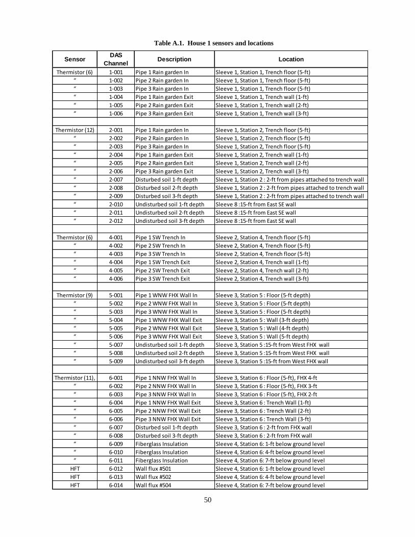
50
Table A.1. House 1 sensors and locations
Thermistor (6) 1-001 Pipe 1 Rain garden In Sleeve 1, Station 1, Trench floor (5-ft)
“ 1-002 Pipe 2 Rain garden In Sleeve 1, Station 1, Trench floor (5-ft)
“ 1-003 Pipe 3 Rain garden In Sleeve 1, Station 1, Trench floor (5-ft)
“ 1-004 Pipe 1 Rain garden Exit Sleeve 1, Station 1, Trench wall (1-ft)
“ 1-005 Pipe 2 Rain garden Exit Sleeve 1, Station 1, Trench wall (2-ft)
“ 1-006 Pipe 3 Rain garden Exit Sleeve 1, Station 1, Trench wall (3-ft)
Thermistor (12) 2-001 Pipe 1 Rain garden In Sleeve 1, Station 2, Trench floor (5-ft)
“ 2-002 Pipe 2 Rain garden In Sleeve 1, Station 2, Trench floor (5-ft)
“ 2-003 Pipe 3 Rain garden In Sleeve 1, Station 2, Trench floor (5-ft)
“ 2-004 Pipe 1 Rain garden Exit Sleeve 1, Station 2, Trench wall (1-ft)
“ 2-005 Pipe 2 Rain garden Exit Sleeve 1, Station 2, Trench wall (2-ft)
“ 2-006 Pipe 3 Rain garden Exit Sleeve 1, Station 2, Trench wall (3-ft)
“ 2-007 Disturbed soil 1-ft depth Sleeve 1, Station 2 : 2-ft from pipes attached to trench wall
“ 2-008 Disturbed soil 2-ft depth Sleeve 1, Station 2 : 2-ft from pipes attached to trench wall
“ 2-009 Disturbed soil 3-ft depth Sleeve 1, Station 2 : 2-ft from pipes attached to trench wall
“ 2-010 Undisturbed soil 1-ft depth Sleeve 8 :15-ft from East SE wall
“ 2-011 Undisturbed soil 2-ft depth Sleeve 8 :15-ft from East SE wall
“ 2-012 Undisturbed soil 3-ft depth Sleeve 8 :15-ft from East SE wall
Thermistor (6) 4-001 Pipe 1 SW Trench In Sleeve 2, Station 4, Trench floor (5-ft)
“ 4-002 Pipe 2 SW Trench In Sleeve 2, Station 4, Trench floor (5-ft)
“ 4-003 Pipe 3 SW Trench In Sleeve 2, Station 4, Trench floor (5-ft)
“ 4-004 Pipe 1 SW Trench Exit Sleeve 2, Station 4, Trench wall (1-ft)
“ 4-005 Pipe 2 SW Trench Exit Sleeve 2, Station 4, Trench wall (2-ft)
“ 4-006 Pipe 3 SW Trench Exit Sleeve 2, Station 4, Trench wall (3-ft)
Thermistor (9) 5-001 Pipe 1 WNW FHX Wall In Sleeve 3, Station 5 : Floor (5-ft depth)
“ 5-002 Pipe 2 WNW FHX Wall In Sleeve 3, Station 5 : Floor (5-ft depth)
“ 5-003 Pipe 3 WNW FHX Wall In Sleeve 3, Station 5 : Floor (5-ft depth)
“ 5-004 Pipe 1 WNW FHX Wall Exit Sleeve 3, Station 5 : Wall (3-ft depth)
“ 5-005 Pipe 2 WNW FHX Wall Exit Sleeve 3, Station 5 : Wall (4-ft depth)
“ 5-006 Pipe 3 WNW FHX Wall Exit Sleeve 3, Station 5 : Wall (5-ft depth)
“ 5-007 Undisturbed soil 1-ft depth Sleeve 3, Station 5 :15-ft from West FHX wall
“ 5-008 Undisturbed soil 2-ft depth Sleeve 3, Station 5 :15-ft from West FHX wall
“ 5-009 Undisturbed soil 3-ft depth Sleeve 3, Station 5 :15-ft from West FHX wall
Thermistor (11), 6-001 Pipe 1 NNW FHX Wall In Sleeve 3, Station 6 : Floor (5-ft), FHX 4-ft
“ 6-002 Pipe 2 NNW FHX Wall In Sleeve 3, Station 6 : Floor (5-ft), FHX 3-ft
“ 6-003 Pipe 3 NNW FHX Wall In Sleeve 3, Station 6 : Floor (5-ft), FHX 2-ft
“ 6-004 Pipe 1 NNW FHX Wall Exit Sleeve 3, Station 6 : Trench Wall (1-ft)
“ 6-005 Pipe 2 NNW FHX Wall Exit Sleeve 3, Station 6 : Trench Wall (2-ft)
“ 6-006 Pipe 3 NNW FHX Wall Exit Sleeve 3, Station 6 : Trench Wall (3-ft)
“ 6-007 Disturbed soil 1-ft depth Sleeve 3, Station 6 : 2-ft from FHX wall
“ 6-008 Disturbed soil 3-ft depth Sleeve 3, Station 6 : 2-ft from FHX wall
“ 6-009 Fiberglass Insulation Sleeve 4, Station 6: 1-ft below ground level
“ 6-010 Fiberglass Insulation Sleeve 4, Station 6: 4-ft below ground level
“ 6-011 Fiberglass Insulation Sleeve 4, Station 6: 7-ft below ground level
HFT 6-012 Wall flux #501 Sleeve 4, Station 6: 1-ft below ground level
HFT 6-013 Wall flux #502 Sleeve 4, Station 6: 4-ft below ground level
HFT 6-014 Wall flux #504 Sleeve 4, Station 6: 7-ft below ground level
LocationSensorDAS
ChannelDescription
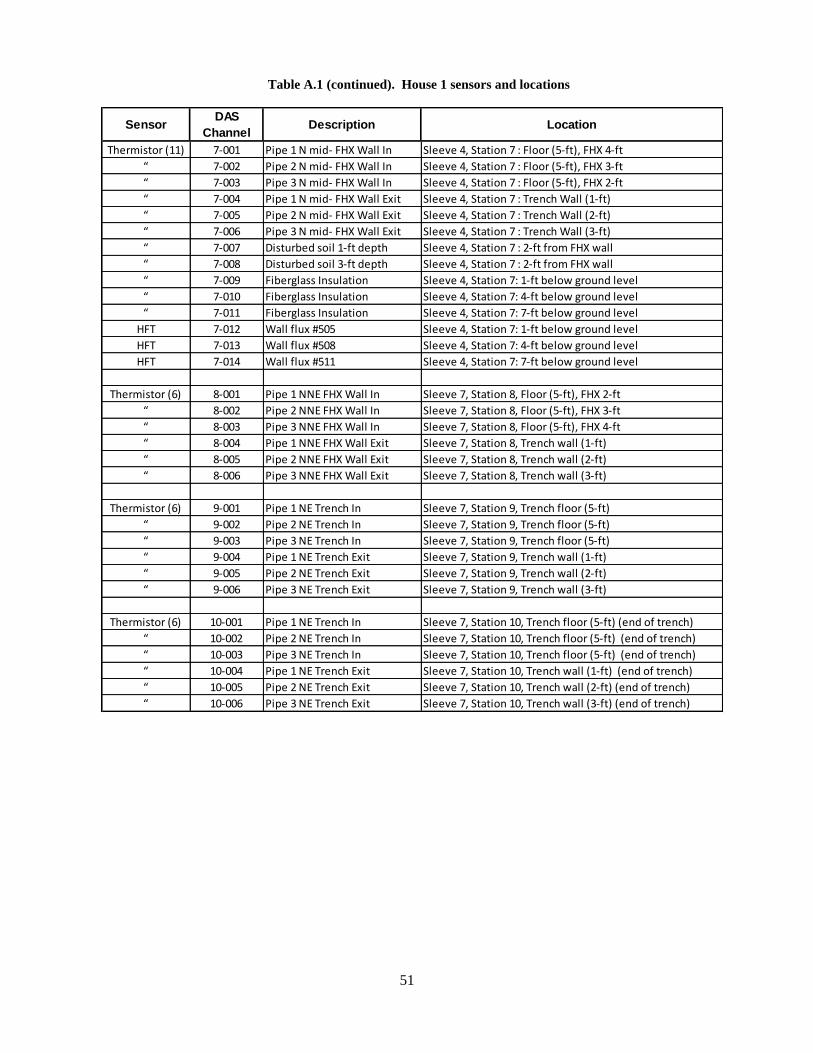
51
Table A.1 (continued). House 1 sensors and locations
Thermistor (11) 7-001 Pipe 1 N mid- FHX Wall In Sleeve 4, Station 7 : Floor (5-ft), FHX 4-ft
“ 7-002 Pipe 2 N mid- FHX Wall In Sleeve 4, Station 7 : Floor (5-ft), FHX 3-ft
“ 7-003 Pipe 3 N mid- FHX Wall In Sleeve 4, Station 7 : Floor (5-ft), FHX 2-ft
“ 7-004 Pipe 1 N mid- FHX Wall Exit Sleeve 4, Station 7 : Trench Wall (1-ft)
“ 7-005 Pipe 2 N mid- FHX Wall Exit Sleeve 4, Station 7 : Trench Wall (2-ft)
“ 7-006 Pipe 3 N mid- FHX Wall Exit Sleeve 4, Station 7 : Trench Wall (3-ft)
“ 7-007 Disturbed soil 1-ft depth Sleeve 4, Station 7 : 2-ft from FHX wall
“ 7-008 Disturbed soil 3-ft depth Sleeve 4, Station 7 : 2-ft from FHX wall
“ 7-009 Fiberglass Insulation Sleeve 4, Station 7: 1-ft below ground level
“ 7-010 Fiberglass Insulation Sleeve 4, Station 7: 4-ft below ground level
“ 7-011 Fiberglass Insulation Sleeve 4, Station 7: 7-ft below ground level
HFT 7-012 Wall flux #505 Sleeve 4, Station 7: 1-ft below ground level
HFT 7-013 Wall flux #508 Sleeve 4, Station 7: 4-ft below ground level
HFT 7-014 Wall flux #511 Sleeve 4, Station 7: 7-ft below ground level
Thermistor (6) 8-001 Pipe 1 NNE FHX Wall In Sleeve 7, Station 8, Floor (5-ft), FHX 2-ft
“ 8-002 Pipe 2 NNE FHX Wall In Sleeve 7, Station 8, Floor (5-ft), FHX 3-ft
“ 8-003 Pipe 3 NNE FHX Wall In Sleeve 7, Station 8, Floor (5-ft), FHX 4-ft
“ 8-004 Pipe 1 NNE FHX Wall Exit Sleeve 7, Station 8, Trench wall (1-ft)
“ 8-005 Pipe 2 NNE FHX Wall Exit Sleeve 7, Station 8, Trench wall (2-ft)
“ 8-006 Pipe 3 NNE FHX Wall Exit Sleeve 7, Station 8, Trench wall (3-ft)
Thermistor (6) 9-001 Pipe 1 NE Trench In Sleeve 7, Station 9, Trench floor (5-ft)
“ 9-002 Pipe 2 NE Trench In Sleeve 7, Station 9, Trench floor (5-ft)
“ 9-003 Pipe 3 NE Trench In Sleeve 7, Station 9, Trench floor (5-ft)
“ 9-004 Pipe 1 NE Trench Exit Sleeve 7, Station 9, Trench wall (1-ft)
“ 9-005 Pipe 2 NE Trench Exit Sleeve 7, Station 9, Trench wall (2-ft)
“ 9-006 Pipe 3 NE Trench Exit Sleeve 7, Station 9, Trench wall (3-ft)
Thermistor (6) 10-001 Pipe 1 NE Trench In Sleeve 7, Station 10, Trench floor (5-ft) (end of trench)
“ 10-002 Pipe 2 NE Trench In Sleeve 7, Station 10, Trench floor (5-ft) (end of trench)
“ 10-003 Pipe 3 NE Trench In Sleeve 7, Station 10, Trench floor (5-ft) (end of trench)
“ 10-004 Pipe 1 NE Trench Exit Sleeve 7, Station 10, Trench wall (1-ft) (end of trench)
“ 10-005 Pipe 2 NE Trench Exit Sleeve 7, Station 10, Trench wall (2-ft) (end of trench)
“ 10-006 Pipe 3 NE Trench Exit Sleeve 7, Station 10, Trench wall (3-ft) (end of trench)
LocationSensorDAS
ChannelDescription
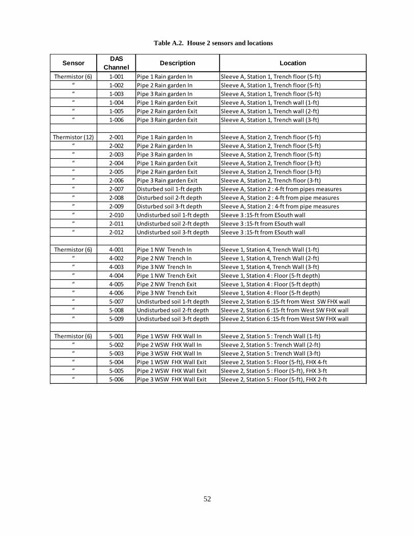
52
Table A.2. House 2 sensors and locations
Thermistor (6) 1-001 Pipe 1 Rain garden In Sleeve A, Station 1, Trench floor (5-ft)
“ 1-002 Pipe 2 Rain garden In Sleeve A, Station 1, Trench floor (5-ft)
“ 1-003 Pipe 3 Rain garden In Sleeve A, Station 1, Trench floor (5-ft)
“ 1-004 Pipe 1 Rain garden Exit Sleeve A, Station 1, Trench wall (1-ft)
“ 1-005 Pipe 2 Rain garden Exit Sleeve A, Station 1, Trench wall (2-ft)
“ 1-006 Pipe 3 Rain garden Exit Sleeve A, Station 1, Trench wall (3-ft)
Thermistor (12) 2-001 Pipe 1 Rain garden In Sleeve A, Station 2, Trench floor (5-ft)
“ 2-002 Pipe 2 Rain garden In Sleeve A, Station 2, Trench floor (5-ft)
“ 2-003 Pipe 3 Rain garden In Sleeve A, Station 2, Trench floor (5-ft)
“ 2-004 Pipe 1 Rain garden Exit Sleeve A, Station 2, Trench floor (3-ft)
“ 2-005 Pipe 2 Rain garden Exit Sleeve A, Station 2, Trench floor (3-ft)
“ 2-006 Pipe 3 Rain garden Exit Sleeve A, Station 2, Trench floor (3-ft)
“ 2-007 Disturbed soil 1-ft depth Sleeve A, Station 2 : 4-ft from pipes measures
“ 2-008 Disturbed soil 2-ft depth Sleeve A, Station 2 : 4-ft from pipe measures
“ 2-009 Disturbed soil 3-ft depth Sleeve A, Station 2 : 4-ft from pipe measures
“ 2-010 Undisturbed soil 1-ft depth Sleeve 3 :15-ft from ESouth wall
“ 2-011 Undisturbed soil 2-ft depth Sleeve 3 :15-ft from ESouth wall
“ 2-012 Undisturbed soil 3-ft depth Sleeve 3 :15-ft from ESouth wall
Thermistor (6) 4-001 Pipe 1 NW Trench In Sleeve 1, Station 4, Trench Wall (1-ft)
“ 4-002 Pipe 2 NW Trench In Sleeve 1, Station 4, Trench Wall (2-ft)
“ 4-003 Pipe 3 NW Trench In Sleeve 1, Station 4, Trench Wall (3-ft)
“ 4-004 Pipe 1 NW Trench Exit Sleeve 1, Station 4 : Floor (5-ft depth)
“ 4-005 Pipe 2 NW Trench Exit Sleeve 1, Station 4 : Floor (5-ft depth)
“ 4-006 Pipe 3 NW Trench Exit Sleeve 1, Station 4 : Floor (5-ft depth)
“ 5-007 Undisturbed soil 1-ft depth Sleeve 2, Station 6 :15-ft from West SW FHX wall
“ 5-008 Undisturbed soil 2-ft depth Sleeve 2, Station 6 :15-ft from West SW FHX wall
“ 5-009 Undisturbed soil 3-ft depth Sleeve 2, Station 6 :15-ft from West SW FHX wall
Thermistor (6) 5-001 Pipe 1 WSW FHX Wall In Sleeve 2, Station 5 : Trench Wall (1-ft)
“ 5-002 Pipe 2 WSW FHX Wall In Sleeve 2, Station 5 : Trench Wall (2-ft)
“ 5-003 Pipe 3 WSW FHX Wall In Sleeve 2, Station 5 : Trench Wall (3-ft)
“ 5-004 Pipe 1 WSW FHX Wall Exit Sleeve 2, Station 5 : Floor (5-ft), FHX 4-ft
“ 5-005 Pipe 2 WSW FHX Wall Exit Sleeve 2, Station 5 : Floor (5-ft), FHX 3-ft
“ 5-006 Pipe 3 WSW FHX Wall Exit Sleeve 2, Station 5 : Floor (5-ft), FHX 2-ft
LocationSensorDAS
ChannelDescription
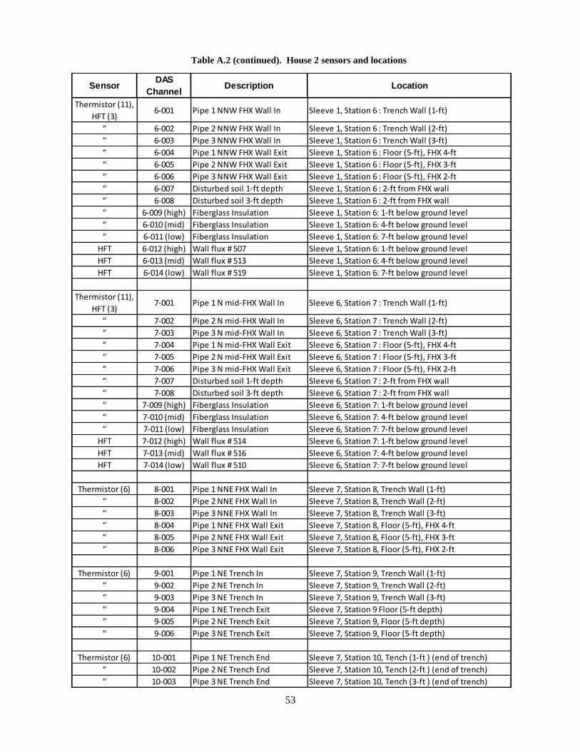
53
Table A.2 (continued). House 2 sensors and locations
Thermistor (11),
HFT (3)6-001 Pipe 1 NNW FHX Wall In Sleeve 1, Station 6 : Trench Wall (1-ft)
“ 6-002 Pipe 2 NNW FHX Wall In Sleeve 1, Station 6 : Trench Wall (2-ft)
“ 6-003 Pipe 3 NNW FHX Wall In Sleeve 1, Station 6 : Trench Wall (3-ft)
“ 6-004 Pipe 1 NNW FHX Wall Exit Sleeve 1, Station 6 : Floor (5-ft), FHX 4-ft
“ 6-005 Pipe 2 NNW FHX Wall Exit Sleeve 1, Station 6 : Floor (5-ft), FHX 3-ft
“ 6-006 Pipe 3 NNW FHX Wall Exit Sleeve 1, Station 6 : Floor (5-ft), FHX 2-ft
“ 6-007 Disturbed soil 1-ft depth Sleeve 1, Station 6 : 2-ft from FHX wall
“ 6-008 Disturbed soil 3-ft depth Sleeve 1, Station 6 : 2-ft from FHX wall
“ 6-009 (high) Fiberglass Insulation Sleeve 1, Station 6: 1-ft below ground level
“ 6-010 (mid) Fiberglass Insulation Sleeve 1, Station 6: 4-ft below ground level
“ 6-011 (low) Fiberglass Insulation Sleeve 1, Station 6: 7-ft below ground level
HFT 6-012 (high) Wall flux # 507 Sleeve 1, Station 6: 1-ft below ground level
HFT 6-013 (mid) Wall flux # 513 Sleeve 1, Station 6: 4-ft below ground level
HFT 6-014 (low) Wall flux # 519 Sleeve 1, Station 6: 7-ft below ground level
Thermistor (11),
HFT (3)7-001 Pipe 1 N mid-FHX Wall In Sleeve 6, Station 7 : Trench Wall (1-ft)
“ 7-002 Pipe 2 N mid-FHX Wall In Sleeve 6, Station 7 : Trench Wall (2-ft)
“ 7-003 Pipe 3 N mid-FHX Wall In Sleeve 6, Station 7 : Trench Wall (3-ft)
“ 7-004 Pipe 1 N mid-FHX Wall Exit Sleeve 6, Station 7 : Floor (5-ft), FHX 4-ft
“ 7-005 Pipe 2 N mid-FHX Wall Exit Sleeve 6, Station 7 : Floor (5-ft), FHX 3-ft
“ 7-006 Pipe 3 N mid-FHX Wall Exit Sleeve 6, Station 7 : Floor (5-ft), FHX 2-ft
“ 7-007 Disturbed soil 1-ft depth Sleeve 6, Station 7 : 2-ft from FHX wall
“ 7-008 Disturbed soil 3-ft depth Sleeve 6, Station 7 : 2-ft from FHX wall
“ 7-009 (high) Fiberglass Insulation Sleeve 6, Station 7: 1-ft below ground level
“ 7-010 (mid) Fiberglass Insulation Sleeve 6, Station 7: 4-ft below ground level
“ 7-011 (low) Fiberglass Insulation Sleeve 6, Station 7: 7-ft below ground level
HFT 7-012 (high) Wall flux # 514 Sleeve 6, Station 7: 1-ft below ground level
HFT 7-013 (mid) Wall flux # 516 Sleeve 6, Station 7: 4-ft below ground level
HFT 7-014 (low) Wall flux # 510 Sleeve 6, Station 7: 7-ft below ground level
Thermistor (6) 8-001 Pipe 1 NNE FHX Wall In Sleeve 7, Station 8, Trench Wall (1-ft)
“ 8-002 Pipe 2 NNE FHX Wall In Sleeve 7, Station 8, Trench Wall (2-ft)
“ 8-003 Pipe 3 NNE FHX Wall In Sleeve 7, Station 8, Trench Wall (3-ft)
“ 8-004 Pipe 1 NNE FHX Wall Exit Sleeve 7, Station 8, Floor (5-ft), FHX 4-ft
“ 8-005 Pipe 2 NNE FHX Wall Exit Sleeve 7, Station 8, Floor (5-ft), FHX 3-ft
“ 8-006 Pipe 3 NNE FHX Wall Exit Sleeve 7, Station 8, Floor (5-ft), FHX 2-ft
Thermistor (6) 9-001 Pipe 1 NE Trench In Sleeve 7, Station 9, Trench Wall (1-ft)
“ 9-002 Pipe 2 NE Trench In Sleeve 7, Station 9, Trench Wall (2-ft)
“ 9-003 Pipe 3 NE Trench In Sleeve 7, Station 9, Trench Wall (3-ft)
“ 9-004 Pipe 1 NE Trench Exit Sleeve 7, Station 9 Floor (5-ft depth)
“ 9-005 Pipe 2 NE Trench Exit Sleeve 7, Station 9, Floor (5-ft depth)
“ 9-006 Pipe 3 NE Trench Exit Sleeve 7, Station 9, Floor (5-ft depth)
Thermistor (6) 10-001 Pipe 1 NE Trench End Sleeve 7, Station 10, Tench (1-ft ) (end of trench)
“ 10-002 Pipe 2 NE Trench End Sleeve 7, Station 10, Tench (2-ft ) (end of trench)
“ 10-003 Pipe 3 NE Trench End Sleeve 7, Station 10, Tench (3-ft ) (end of trench)
LocationSensorDAS
ChannelDescription