Four-Bar Linkage Synthesis Using Non-ConvexOptimization

Vincent Goulet1, Wei Li2, Hyunmin Cheong2, Francesco Iorio2, and Claude-GuyQuimper1

1 Université Laval2 Autodesk Research

Abstract. We show how four-bar linkages can be designed using non-convex op-timization techniques. Our generative design software takes as input a curve thatneeds to be reproduced by a four-bar linkage and outputs the best assembly thatapproximates this curve. We model the problem using quadratic constraints andshow how redundant constraints help to solve the problem. We also provide analgorithm that samples the curve based on its characteristics. Experiments showthat our software is faster and more precise than existing systems. The currentwork is part of a larger generative design initiative at Autodesk Research.

1 Introduction

A mechanism is an arrangement of machine parts that generates a specified motion. Thesynthesis of a mechanism is the process of determining the position, the orientation, andother parametric properties of parts according to constraints governing their alignmentor motion. The design of mechanisms has greatly benefited from the advent of com-puter techniques. Computer-aided design and engineering software (CAD/CAE) havebeen widely used in the documentation, analysis, and optimization of designs. Though,still nowadays, the existing technologies and tools lack a function for automated mech-anism synthesis. Creating mechanisms that meet specified motion and geometric re-quirements demands highly trained expert designers. As the available computing powerkeeps growing, so does the interest in the development of generative design tools.

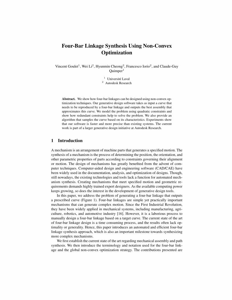
In this paper, we address the problem of generating a four-bar linkage that outputsa prescribed curve (Figure 1). Four-bar linkages are simple yet practically importantmechanisms that can generate complex motion. Since the First Industrial Revolution,they have been widely applied in mechanical systems, including manufacturing, agri-culture, robotics, and automotive industry [16]. However, it is a laborious process tomanually design a four-bar linkage based on a target curve. The current state of the artof four-bar linkage design is a time consuming process, and the results often lack op-timality or generality. Hence, this paper introduces an automated and efficient four-barlinkage synthesis approach, which is also an important milestone towards synthesizingmore complex mechanisms.

We first establish the current state of the art regarding mechanical assembly and pathsynthesis. We then introduce the terminology and notation used for the four-bar link-age and the global non-convex optimization strategy. The contributions presented are

Fig. 1. A four-bar linkage and output coupler curve

the feature identification sampling technique, the four-bar linkage quadratic model, thespecial constraint on the area of the curve, and the design software developed. Resultsemphasizing the speed and quality of our method follow along with a discussion.

2 Related Work

2.1 Mechanical Assembly

A long standing challenge of mechanical design is the automation of design synthe-sis tasks [21]. Existing mechanism synthesis methods include systematic search [22,17], machine-learning based approaches [8], stochastic search [26] and graph-basedapproach [18, 20]. However, to the best of our knowledge, existing generative designapproaches still lack the generality or performance to be practical.

2.2 Path Synthesis of Four-Bar Linkage

Without a computer-aided approach, a human designer typically uses prior knowledgeand/or atlases of coupler curves to identify a candidate linkage to produce the desiredcurve [16]. Then the chosen linkage is modified until it is satisfactory [25].

Analytical approaches formulate the four-bar linkage constraints, solve the problemand return exact solutions [19, 24]. They require a set of points or positions input bythe user, which can be challenging to provide. In many cases, there is no mechanismthat can produce exactly the desired path. In fact, although the mechanism found goesthrough the specified points, it may not go through the desired curve (see Fig. 8 for anexample). Also, analytical approaches are limited to solving problems with five or lesstarget points, (see [14] and the references therein).

Alternatively, numerical methods are used to synthesize approximate mechanismswith acceptable tolerance between the input path and the coupler curve. Genetic algo-rithms have been widely applied to the four-bar mechanism synthesis problem [7, 2].Genetic algorithms and other stochastic search methods [6] have the same limitation –there is no assurance that they will find a global optimum. Also, because the objectivefunction of four-bar mechanisms is highly constrained, the typical evolutionary algo-rithms have to choose a very large number of initial population so that a considerableamount of them can play in the next iteration. This technique unnecessarily increasesCPU time and reserves a large amount of memory during the computing iterations. Thelack of consistency also makes it challenging for performance evaluation.

Machine-learning approaches [8, 25] store a large number of coupler curves in adatabase. Automated procedures for fitting coupler curves are used to locate potentiallinkage solutions from the database. Neural network [12] and sequential quadratic pro-gramming [8] can be used to match coupler curves. However, such an approach requiresbuilding a large linkage database. Another limitation is that the quality of the generatedmotion directly depends on the mechanisms in the database and sampling techniques.

3 Preliminaries

3.1 Mechanical Linkage

A mechanical linkage is a set of rigid bodies, called links, connected by joints. Thoughmany types of joints exist, we herein only consider the revolute joint or pivot, whichallows for one degree of freedom rotation. This paper focuses on the two-dimensionalfour-bar linkage (Figure 1), made of four links in a closed loop. The joints A, B, C andD are pivots. The positions of A and B are fixed. The motion of point E is the outputof the mechanism, therefore it is called the end effector. The link AB, called the frame,cannot move. The link AC, called the crank, drives the motion of the linkage. The linkBD is driven back and forth about B and is called the rocker. The link CDE, called thecoupler, couples the rocker to the crank. The path traced by E over a full rotation of thecrank is called the coupler curve. A four-bar linkage is collinear if point E is alignedwith C and D. A linkage is Grashof if one link is able to fully rotate. We assume thiscondition is met and the crank AC can fully rotate.

3.2 Non-Convex Global Optimization

Mathematical optimization aims at finding good solutions to a problem according tosome user-defined criteria. Global optimization is a family of techniques that guaranteethat the solutions returned are absolutely optimal. These techniques often consist ofrelaxing the problem to a form efficiently solvable to optimality. This relaxed solutionprovides a bound for branch and bound search.

To be computable, the global optimization problem is modelled mathematically. Themodel consists of a set of variables, a set of constraints that need to be satisfied, and anobjective function. Each variable has a domain, a set of all values it can be assigned.

The solver takes as input the model and finds suitable values for all variables, suchthat constraints are satisfied and the objective is optimized. Solvers are available for awide range of applications and can be categorized by the types of variables they canhandle, whether Boolean, integer, or real. Solvers can also be categorized by the typesof functions they can handle, whether logic, linear, convex, or non-convex.

Modelling a four-bar linkage requires real variables and non-convex constraints.The global optimization solver Couenne [5] is specialized in both regards, and is thesolver used for all experimentation presented. It was chosen over related candidatesof comparable performance such as Baron [23] and AlphaBB [4] because it is opensource. The constraint solver IBEX [1] was also considered but did not show sufficientperformance. Other considered continuous solvers include RealPaver [10], SCIP [3]and LindoAPI [15].

Non-convex problems are difficult to solve even for the best available software.Couenne combines many techniques from constraint programming and other optimiza-tion subfields. It uses constraint propagation and interval arithmetic to achieve boundstightening on each variable [5], therefore reducing the search space. It relaxes the non-linear constraints into linear envelopes. It uses branch and bound to create more tightlybounded subproblems. By adding redundant constraints, this envelope is further tight-ened. Whether redundant constraints make the solving faster depends on their numberand complexity. Testing is required for validation. Couenne feeds the linear problem toCPLEX [13] to compute the solution to the relaxation.

4 Contribution

We developed a strategy to effectively design four-bar linkages outputting a desiredcurve using non-convex optimization. The benefits of this application are that the syn-thesis of the continuous curve is accurate, fast, and deterministic. The time frame ofthis project spanned six months. The first two months were used to survey the avail-able technology. The last four months were used to develop the model and strategy.We modelled the mechanism using its geometric properties, keeping in mind the possi-ble generalization to mechanisms of higher complexity, and a novel cut (or redundantconstraint) was developed using the area of the curve. We also designed a novel pointsampling technique. We implemented this strategy in a simple design software.

4.1 Fitness Metric

We aim at designing a four-bar linkage which replicates as tightly as possible a contin-uous curve. To make this problem tractable for the constraint solver, we strategicallysample the curve using the technique describe in Sec. 4.2. The model described inSec. 4.3 minimizes a single variable e which represents the maximum distance fromthe curve to a sample point. We sample the curve with as little points as possible tokeep the search space small. Note that the solver could return a solution with zero error,meaning the solution curve reaches all sample points, and yet not match the input curve,as shown in Fig. 8. In general, it is necessary to evaluate how well the continuous inputcurve matches the output curve after it is returned, regardless of the objective value.

Several well-established curve matching metrics exist. The Hausdorff distance [11]d is the greatest distance from any point on the curves to the closest point on the othercurve. To render the metric independent of the size of the curves, we normalize it withthe greatest x- or y-dimension of the curve. The normalized Hausdorff distance is hereindesignated as Q. In compliance with Fig. 2, the equation for Q is:

Q =d

max (∆x,∆y)

Figure 3 shows matching curves for different Q values. A Q value of 0 is a perfectmatch. The user can define a threshold T under which the curves are considered a goodmatch. It is worth noting that Q does not consider the course of the curve, which mightresult in undesired matches, especially when a curve self-crosses. However, features ofthe model such as the area constraint discussed in Sec. 4.4 make these events unlikely.

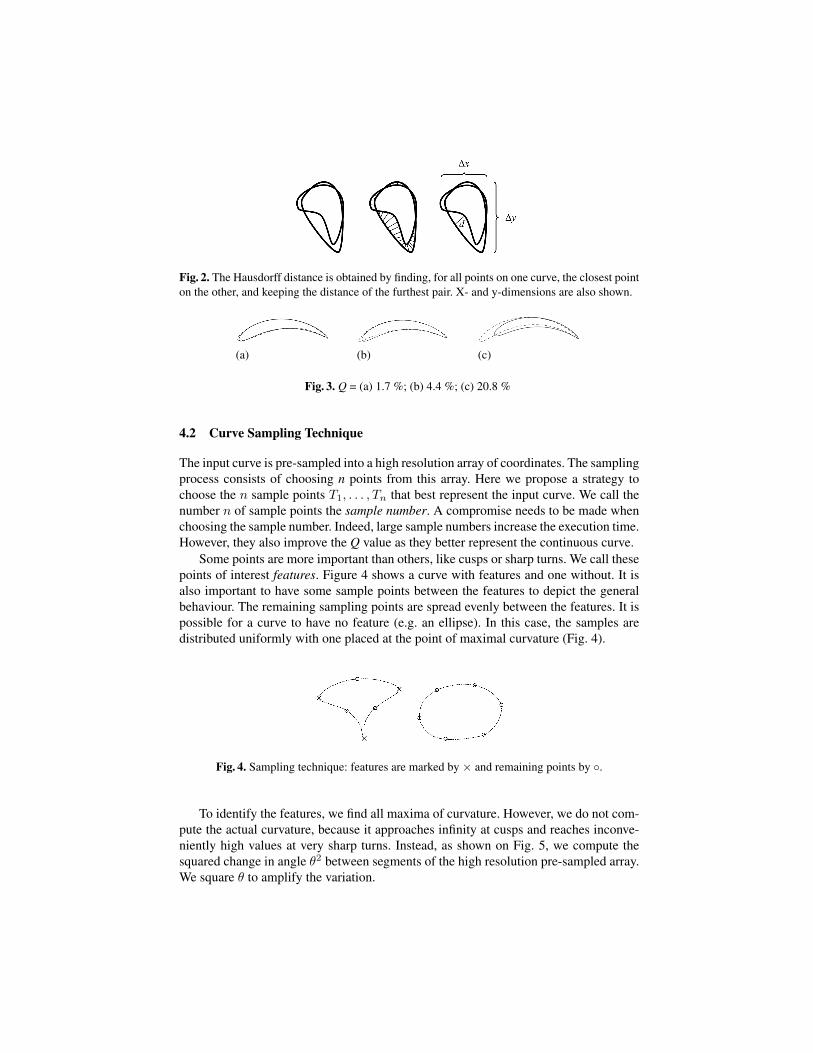
Fig. 2. The Hausdorff distance is obtained by finding, for all points on one curve, the closest pointon the other, and keeping the distance of the furthest pair. X- and y-dimensions are also shown.

(a) (b) (c)

Fig. 3. Q = (a) 1.7 %; (b) 4.4 %; (c) 20.8 %

4.2 Curve Sampling Technique

The input curve is pre-sampled into a high resolution array of coordinates. The samplingprocess consists of choosing n points from this array. Here we propose a strategy tochoose the n sample points T1, . . . , Tn that best represent the input curve. We call thenumber n of sample points the sample number. A compromise needs to be made whenchoosing the sample number. Indeed, large sample numbers increase the execution time.However, they also improve the Q value as they better represent the continuous curve.

Some points are more important than others, like cusps or sharp turns. We call thesepoints of interest features. Figure 4 shows a curve with features and one without. It isalso important to have some sample points between the features to depict the generalbehaviour. The remaining sampling points are spread evenly between the features. It ispossible for a curve to have no feature (e.g. an ellipse). In this case, the samples aredistributed uniformly with one placed at the point of maximal curvature (Fig. 4).

Fig. 4. Sampling technique: features are marked by × and remaining points by ◦.

To identify the features, we find all maxima of curvature. However, we do not com-pute the actual curvature, because it approaches infinity at cusps and reaches inconve-niently high values at very sharp turns. Instead, as shown on Fig. 5, we compute thesquared change in angle θ2 between segments of the high resolution pre-sampled array.We square θ to amplify the variation.

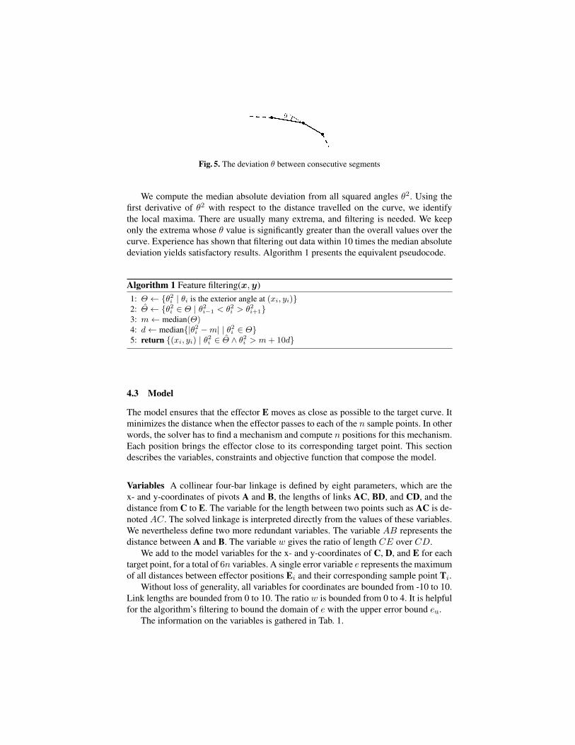
Fig. 5. The deviation θ between consecutive segments

We compute the median absolute deviation from all squared angles θ2. Using thefirst derivative of θ2 with respect to the distance travelled on the curve, we identifythe local maxima. There are usually many extrema, and filtering is needed. We keeponly the extrema whose θ value is significantly greater than the overall values over thecurve. Experience has shown that filtering out data within 10 times the median absolutedeviation yields satisfactory results. Algorithm 1 presents the equivalent pseudocode.

Algorithm 1 Feature filtering(x,y)1: Θ ← {θ2i | θi is the exterior angle at (xi, yi)}2: Θ̂ ← {θ2i ∈ Θ | θ2i−1 < θ2i > θ2i+1}3: m← median(Θ)4: d← median{|θ2i −m| | θ2i ∈ Θ}5: return {(xi, yi) | θ2i ∈ Θ̂ ∧ θ2i > m+ 10d}

4.3 Model

The model ensures that the effector E moves as close as possible to the target curve. Itminimizes the distance when the effector passes to each of the n sample points. In otherwords, the solver has to find a mechanism and compute n positions for this mechanism.Each position brings the effector close to its corresponding target point. This sectiondescribes the variables, constraints and objective function that compose the model.

Variables A collinear four-bar linkage is defined by eight parameters, which are thex- and y-coordinates of pivots A and B, the lengths of links AC, BD, and CD, and thedistance from C to E. The variable for the length between two points such as AC is de-noted AC. The solved linkage is interpreted directly from the values of these variables.We nevertheless define two more redundant variables. The variable AB represents thedistance between A and B. The variable w gives the ratio of length CE over CD.

We add to the model variables for the x- and y-coordinates of C, D, and E for eachtarget point, for a total of 6n variables. A single error variable e represents the maximumof all distances between effector positions Ei and their corresponding sample point Ti.

Without loss of generality, all variables for coordinates are bounded from -10 to 10.Link lengths are bounded from 0 to 10. The ratio w is bounded from 0 to 4. It is helpfulfor the algorithm’s filtering to bound the domain of e with the upper error bound eu.

The information on the variables is gathered in Tab. 1.

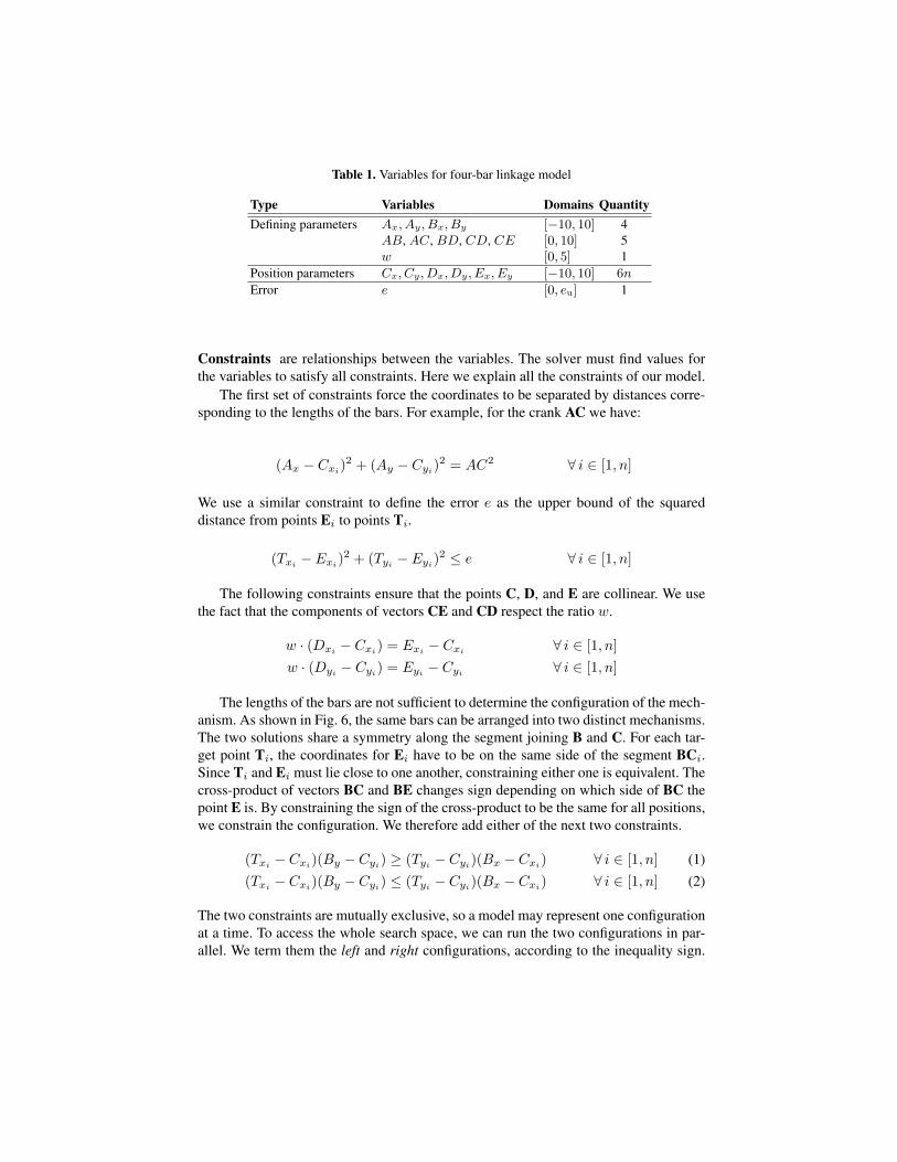
Table 1. Variables for four-bar linkage model

Type Variables Domains QuantityDefining parameters Ax, Ay, Bx, By [−10, 10] 4

AB, AC, BD, CD, CE [0, 10] 5w [0, 5] 1

Position parameters Cx, Cy, Dx, Dy, Ex, Ey [−10, 10] 6n

Error e [0, eu] 1

Constraints are relationships between the variables. The solver must find values forthe variables to satisfy all constraints. Here we explain all the constraints of our model.

The first set of constraints force the coordinates to be separated by distances corre-sponding to the lengths of the bars. For example, for the crank AC we have:

(Ax − Cxi)2 + (Ay − Cyi

)2 = AC2 ∀ i ∈ [1, n]

We use a similar constraint to define the error e as the upper bound of the squareddistance from points Ei to points Ti.

(Txi− Exi

)2 + (Tyi− Eyi

)2 ≤ e ∀ i ∈ [1, n]

The following constraints ensure that the points C, D, and E are collinear. We usethe fact that the components of vectors CE and CD respect the ratio w.

w · (Dxi− Cxi

) = Exi− Cxi

∀ i ∈ [1, n]

w · (Dyi− Cyi

) = Eyi− Cyi

∀ i ∈ [1, n]

The lengths of the bars are not sufficient to determine the configuration of the mech-anism. As shown in Fig. 6, the same bars can be arranged into two distinct mechanisms.The two solutions share a symmetry along the segment joining B and C. For each tar-get point Ti, the coordinates for Ei have to be on the same side of the segment BCi.Since Ti and Ei must lie close to one another, constraining either one is equivalent. Thecross-product of vectors BC and BE changes sign depending on which side of BC thepoint E is. By constraining the sign of the cross-product to be the same for all positions,we constrain the configuration. We therefore add either of the next two constraints.

(Txi − Cxi)(By − Cyi) ≥ (Tyi − Cyi)(Bx − Cxi) ∀ i ∈ [1, n] (1)(Txi − Cxi)(By − Cyi) ≤ (Tyi − Cyi)(Bx − Cxi) ∀ i ∈ [1, n] (2)

The two constraints are mutually exclusive, so a model may represent one configurationat a time. To access the whole search space, we can run the two configurations in par-allel. We term them the left and right configurations, according to the inequality sign.

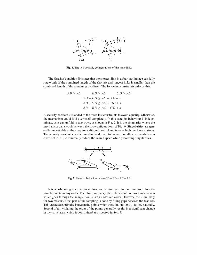
Fig. 6. The two possible configurations of the same links

The Grashof condition [9] states that the shortest link in a four-bar linkage can fullyrotate only if the combined length of the shortest and longest links is smaller than thecombined length of the remaining two links. The following constraints enforce this:

AB ≥ AC BD ≥ AC CD ≥ ACCD +BD ≥ AC +AB + s

AB + CD ≥ AC +BD + s

AB +BD ≥ AC + CD + s

A security constant s is added to the three last constraints to avoid equality. Otherwise,the mechanism could fold over itself completely. In this state, its behaviour is indeter-minate, as it can unfold in two ways, as shown in Fig. 7. It is the singularity where themechanism can switch between the two configurations of Fig. 6. Singularities are gen-erally undesirable as they require additional control and involve high mechanical stress.The security constant s can be tuned to the desired tolerance. For all experiments hereins was set to 0.1, to minimally reduce the search space while preventing singularities.

Fig. 7. Singular behaviour when CD + BD = AC + AB

It is worth noting that the model does not require the solution found to follow thesample points in any order. Therefore, in theory, the solver could return a mechanismwhich goes through the sample points in an undesired order. However, this is unlikelyfor two reasons. First, part of the sampling is done by filling gaps between the features.This creates a continuity between the points which the solutions tend to follow naturally.Second of all, violating the order of the points generally results in a significant changein the curve area, which is constrained as discussed in Sec. 4.4.

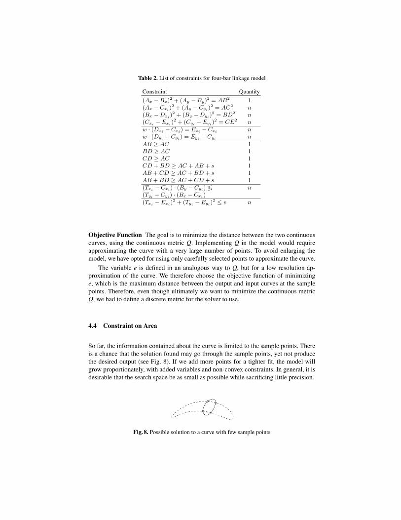
Table 2. List of constraints for four-bar linkage model

Constraint Quantity(Ax −Bx)2 + (Ay −By)2 = AB2 1(Ax − Cxi)

2 + (Ay − Cyi)2 = AC2 n

(Bx −Dxi)2 + (By −Dyi)

2 = BD2 n(Cxi − Exi)

2 + (Cyi − Eyi)2 = CE2 n

w · (Dxi − Cxi) = Exi − Cxi nw · (Dyi − Cyi) = Eyi − Cyi n

AB ≥ AC 1BD ≥ AC 1CD ≥ AC 1CD +BD ≥ AC +AB + s 1AB + CD ≥ AC +BD + s 1AB +BD ≥ AC + CD + s 1(Txi − Cxi) · (By − Cyi) ≶ n(Tyi − Cyi) · (Bx − Cxi)

(Txi − Exi)2 + (Tyi − Eyi)

2 ≤ e n

Objective Function The goal is to minimize the distance between the two continuouscurves, using the continuous metric Q. Implementing Q in the model would requireapproximating the curve with a very large number of points. To avoid enlarging themodel, we have opted for using only carefully selected points to approximate the curve.

The variable e is defined in an analogous way to Q, but for a low resolution ap-proximation of the curve. We therefore choose the objective function of minimizinge, which is the maximum distance between the output and input curves at the samplepoints. Therefore, even though ultimately we want to minimize the continuous metricQ, we had to define a discrete metric for the solver to use.

4.4 Constraint on Area

So far, the information contained about the curve is limited to the sample points. Thereis a chance that the solution found may go through the sample points, yet not producethe desired output (see Fig. 8). If we add more points for a tighter fit, the model willgrow proportionately, with added variables and non-convex constraints. In general, it isdesirable that the search space be as small as possible while sacrificing little precision.

Fig. 8. Possible solution to a curve with few sample points

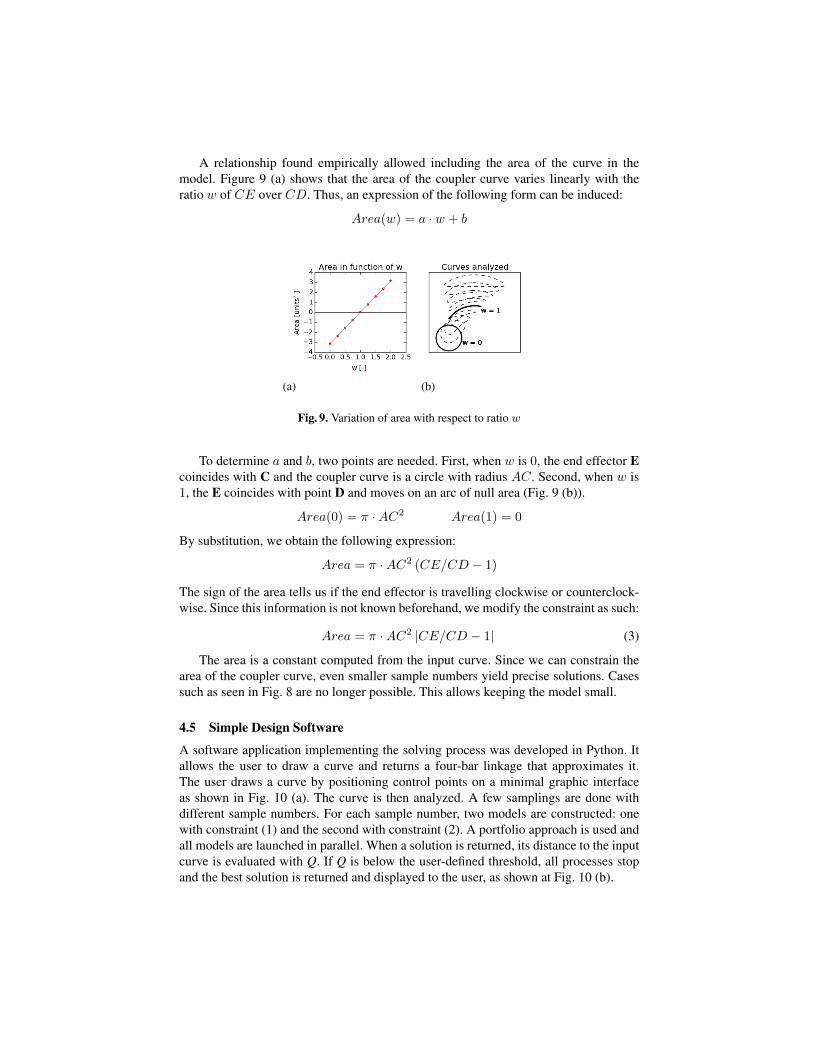
A relationship found empirically allowed including the area of the curve in themodel. Figure 9 (a) shows that the area of the coupler curve varies linearly with theratio w of CE over CD. Thus, an expression of the following form can be induced:

Area(w) = a · w + b

(a) (b)

Fig. 9. Variation of area with respect to ratio w

To determine a and b, two points are needed. First, when w is 0, the end effector Ecoincides with C and the coupler curve is a circle with radius AC. Second, when w is1, the E coincides with point D and moves on an arc of null area (Fig. 9 (b)).

Area(0) = π ·AC2 Area(1) = 0

By substitution, we obtain the following expression:

Area = π ·AC2 (CE/CD − 1)

The sign of the area tells us if the end effector is travelling clockwise or counterclock-wise. Since this information is not known beforehand, we modify the constraint as such:

Area = π ·AC2 |CE/CD − 1| (3)

The area is a constant computed from the input curve. Since we can constrain thearea of the coupler curve, even smaller sample numbers yield precise solutions. Casessuch as seen in Fig. 8 are no longer possible. This allows keeping the model small.

4.5 Simple Design Software

A software application implementing the solving process was developed in Python. Itallows the user to draw a curve and returns a four-bar linkage that approximates it.The user draws a curve by positioning control points on a minimal graphic interfaceas shown in Fig. 10 (a). The curve is then analyzed. A few samplings are done withdifferent sample numbers. For each sample number, two models are constructed: onewith constraint (1) and the second with constraint (2). A portfolio approach is used andall models are launched in parallel. When a solution is returned, its distance to the inputcurve is evaluated with Q. If Q is below the user-defined threshold, all processes stopand the best solution is returned and displayed to the user, as shown at Fig. 10 (b).

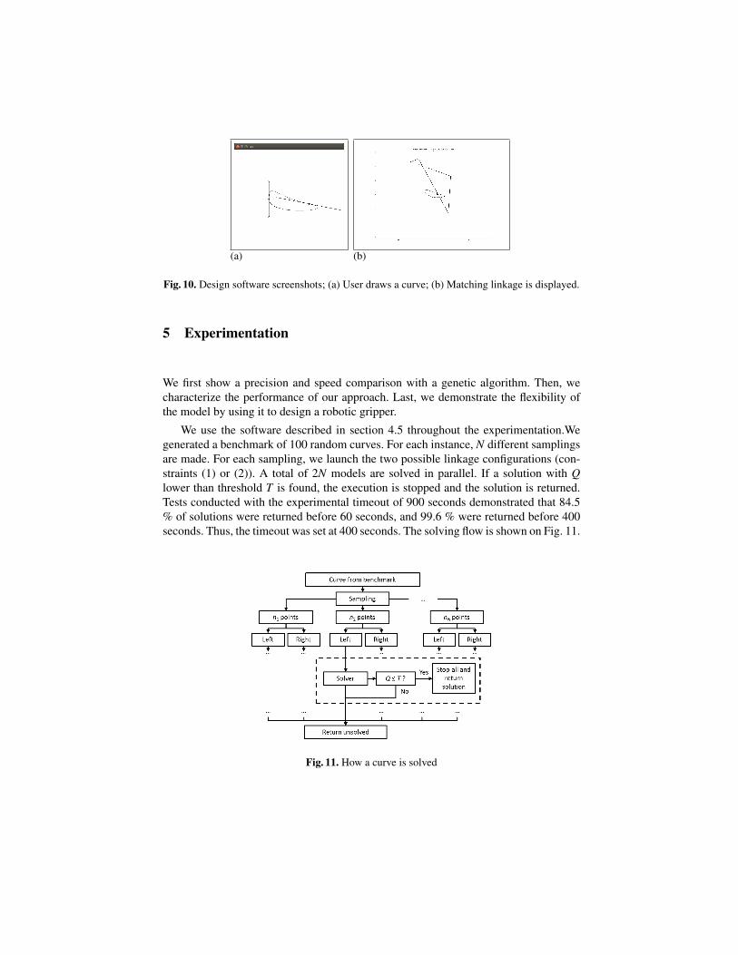
(a) (b)

Fig. 10. Design software screenshots; (a) User draws a curve; (b) Matching linkage is displayed.

5 Experimentation

We first show a precision and speed comparison with a genetic algorithm. Then, wecharacterize the performance of our approach. Last, we demonstrate the flexibility ofthe model by using it to design a robotic gripper.

We use the software described in section 4.5 throughout the experimentation.Wegenerated a benchmark of 100 random curves. For each instance, N different samplingsare made. For each sampling, we launch the two possible linkage configurations (con-straints (1) or (2)). A total of 2N models are solved in parallel. If a solution with Qlower than threshold T is found, the execution is stopped and the solution is returned.Tests conducted with the experimental timeout of 900 seconds demonstrated that 84.5% of solutions were returned before 60 seconds, and 99.6 % were returned before 400seconds. Thus, the timeout was set at 400 seconds. The solving flow is shown on Fig. 11.

Fig. 11. How a curve is solved

5.1 Benchmark

The benchmark consists of 100 coupler curves of randomly generated linkages. Thelinkages were generated within the search space of the model. The curves are resized tofit inside a 4 by 4 units square centred at the origin. All curves measure at least 1 unitat their widest. This benchmark spans a wide range of shapes in the search space of ourmodel, which all possess at least one solution. Some curves are presented at Fig. 12.

Fig. 12. Example curves from the benchmark

5.2 Results

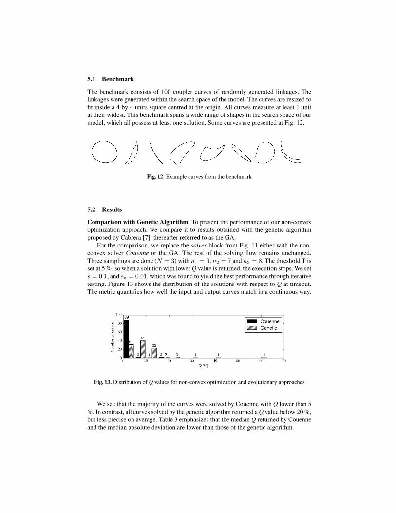
Comparison with Genetic Algorithm To present the performance of our non-convexoptimization approach, we compare it to results obtained with the genetic algorithmproposed by Cabrera [7], thereafter referred to as the GA.

For the comparison, we replace the solver block from Fig. 11 either with the non-convex solver Couenne or the GA. The rest of the solving flow remains unchanged.Three samplings are done (N = 3) with n1 = 6, n2 = 7 and n3 = 8. The threshold T isset at 5 %, so when a solution with lower Q value is returned, the execution stops. We sets = 0.1, and eu = 0.01, which was found to yield the best performance through iterativetesting. Figure 13 shows the distribution of the solutions with respect to Q at timeout.The metric quantifies how well the input and output curves match in a continuous way.

Fig. 13. Distribution of Q values for non-convex optimization and evolutionary approaches

We see that the majority of the curves were solved by Couenne with Q lower than 5%. In contrast, all curves solved by the genetic algorithm returned a Q value below 20 %,but less precise on average. Table 3 emphasizes that the median Q returned by Couenneand the median absolute deviation are lower than those of the genetic algorithm.

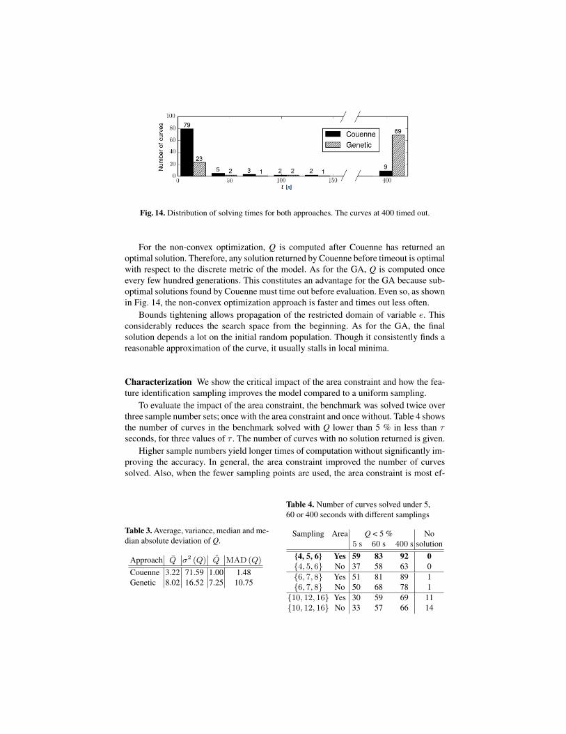
Fig. 14. Distribution of solving times for both approaches. The curves at 400 timed out.

For the non-convex optimization, Q is computed after Couenne has returned anoptimal solution. Therefore, any solution returned by Couenne before timeout is optimalwith respect to the discrete metric of the model. As for the GA, Q is computed onceevery few hundred generations. This constitutes an advantage for the GA because sub-optimal solutions found by Couenne must time out before evaluation. Even so, as shownin Fig. 14, the non-convex optimization approach is faster and times out less often.

Bounds tightening allows propagation of the restricted domain of variable e. Thisconsiderably reduces the search space from the beginning. As for the GA, the finalsolution depends a lot on the initial random population. Though it consistently finds areasonable approximation of the curve, it usually stalls in local minima.

Characterization We show the critical impact of the area constraint and how the fea-ture identification sampling improves the model compared to a uniform sampling.

To evaluate the impact of the area constraint, the benchmark was solved twice overthree sample number sets; once with the area constraint and once without. Table 4 showsthe number of curves in the benchmark solved with Q lower than 5 % in less than τseconds, for three values of τ . The number of curves with no solution returned is given.

Higher sample numbers yield longer times of computation without significantly im-proving the accuracy. In general, the area constraint improved the number of curvessolved. Also, when the fewer sampling points are used, the area constraint is most ef-

Table 3. Average, variance, median and me-dian absolute deviation of Q.

Approach Q̄ σ2 (Q) Q̃ MAD (Q)

Couenne 3.22 71.59 1.00 1.48Genetic 8.02 16.52 7.25 10.75

Table 4. Number of curves solved under 5,60 or 400 seconds with different samplings

Sampling Area Q < 5 % No5 s 60 s 400 s solution

{4, 5, 6} Yes 59 83 92 0{4, 5, 6} No 37 58 63 0{6, 7, 8} Yes 51 81 89 1{6, 7, 8} No 50 68 78 1{10, 12, 16} Yes 30 59 69 11{10, 12, 16} No 33 57 66 14

ficient. Without the area constraint, the software performs best with sample numbers{6, 7, 8}. With the area constraint, lower sample numbers yield a better performance.

The feature identification sampling is compared to a uniform sampling with no anal-ysis of the curve. The experiment was conducted with sets of sample numbers {4, 5, 6}and {6, 7, 8}. Figure 15 shows how the sampling affects the distribution of Q.

(a) (b)

Fig. 15. Distribution of Qs over benchmark with both sampling techniques; (a) sample numbers{4, 5, 6}; (b) sample numbers {6, 7, 8}

For both sets of sample numbers, the feature identification brought the Q distribu-tion closer to 0 %. This shows that without increasing the complexity of the model,choosing points strategically can help achieve greater precision.

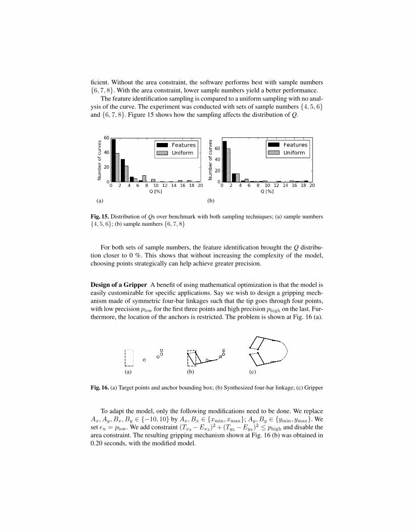
Design of a Gripper A benefit of using mathematical optimization is that the model iseasily customizable for specific applications. Say we wish to design a gripping mech-anism made of symmetric four-bar linkages such that the tip goes through four points,with low precision plow for the first three points and high precision phigh on the last. Fur-thermore, the location of the anchors is restricted. The problem is shown at Fig. 16 (a).

(a) (b) (c)

Fig. 16. (a) Target points and anchor bounding box; (b) Synthesized four-bar linkage; (c) Gripper

To adapt the model, only the following modifications need to be done. We replaceAx, Ay, Bx, By ∈ {−10, 10} by Ax, Bx ∈ {xmin, xmax}; Ay, By ∈ {ymin, ymax}. Weset eu = plow. We add constraint (Tx3

−Ex3)2+(Ty3

−Ey3)2 ≤ phigh and disable the

area constraint. The resulting gripping mechanism shown at Fig. 16 (b) was obtained in0.20 seconds, with the modified model.

5.3 Discussion

Our software can quickly and accurately synthesize collinear four-bar linkages for givencoupler curves. Indeed, the speeds reached are suitable for interactive applications. Be-cause we use a non-convex optimization solver, our approach is flexible and can be read-ily adjusted to meet specific needs or different goals. Unlike analytical approaches [19,24], we are not limited by the number of target points to reach. Moreover, the areaconstraint allows the solver to extrapolate between the target points.

Our method aims at matching a continuous curve rather than a discrete set of targetpoints. However, many related works [7, 6] focus on matching target points. Our resultsshow capabilities in both goals. Indeed, the distance to the target point is bounded bythe error, which cannot be higher than eu or to a maximum of 1 % of the size of thecurve. Any solution discussed matched its target points at least to this precision.

Our approach also presents benefits compared to machine-learning approaches. Adatabase cannot guarantee coverage of the whole search space. With our approach, thesearch space is fully explorable and only limited by user-defined restrictions.

Though we focused on minimizing the error, this can be easily changed by replacingthe objective function. One could minimize the sum of dimensions, the area of thecoupler curve, or the difference of area between the input curve and the output curve.

5.4 Future Work

The software usability could be improved by providing tools to edit constraints.Our software could extend to four-bar linkages where points C, D and E are not

collinear. Difficulties include more symmetric configurations and the generalization ofthe area constraint. Joints such as sliders and complex mechanisms such as geared fiveand six-bar mechanisms could be modelled. 3D-mechanisms could also be tackled. Oursoftware could be combined with other design analyses such as stress analysis. Multiplelinkages could be linked to a gearing software for timing control. Finally, the modelcould be generated as the user defines his own mechanisms by adding bars and joints.

6 Conclusion

The current state of the art of four-bar linkage synthesis is limited in speed, memoryconsumption, lack of optimality or lack of generality. Our paper contributes an im-proved method to the general and fast solving of mechanical linkages. We showed howto accurately solve complete coupler curves in a short time for collinear four-bar link-ages using non-convex optimization. For closed curves, a novel constraint can leveragethe area of the curve for increased accuracy and performance. For our best model, 90 %of the curves could be solved under 400 seconds, 59 % of which below 5 seconds.

Our approach was implemented in simple software where a user can enter a curveand visualize the solution found. This milestone paves the way for modelling mecha-nisms of increased complexity such as the general four-bar linkage or five-bar linkages.It also provides a very flexible basis for solving four-bar linkages with various con-straints or different objectives.

References

1. Ibex library online documentation. http://www.ibex-lib.org/doc/. Accessed: 2016-06-28.2. SK Acharyya and M Mandal. Performance of eas for four-bar linkage synthesis. Mechanism

and Machine Theory, 44(9):1784–1794, 2009.3. Tobias Achterberg. Scip: Solving constraint integer programs. Mathematical Programming

Computation, 1(1):1–41, 2009. http://mpc.zib.de/index.php/MPC/article/view/4.4. I.P. Androulakis, C.D. Maranas, and C.A. FLOUDAS. alphabb: A global optimization

method for general constrained nonconvex problems, 1995.5. P. Belotti, J. Lee, L. Liberti, F. Margot, and A. Wächter. Branching and bounds tightening

techniques for non-convex MINLP. Optimization Methods and Software, 24(4-5):597–634,2009.

6. Radovan R. Bulatovic and Stevan R. Djordjevic. Optimal synthesis of a four-bar linkage bymethod of controlled deviation. Theoretical and applied mechanics, 31(3-4):265–280, 2004.

7. J. A. Cabrera, A. Simon, and M. Prado. Optimal synthesis of mechanisms with geneticalgorithms. Mechanism and Machine theory, 37(10):1165–1177, 2002.

8. Stelian Coros, Bernhard Thomaszewski, Gioacchino Noris, Shinjiro Sueda, Moira Forberg,Robert W. Sumner, Wojciech Matusik, and Bernd Bickel. Computational design of mechan-ical characters. ACM Trans. Graph., 32(4):83:1–83:12, July 2013.

9. Evert Albertus Dijksman. Motion geometry of mechanisms. CUP Archive, 1976.10. Laurent Granvilliers and Frédéric Benhamou. Algorithm 852: RealPaver: an interval solver

using constraint satisfaction techniques. ACM Transactions on Mathematical Software,32(1):138–156, 2006.

11. Wilh Groß. Grundzüge der mengenlehre. Monatshefte für Mathematik, 26(1):A34–A35,1915.

12. D. A. Hoeltzel and Wei-Hua Chieng. Pattern matching synthesis as an automated approachto mechanism design. Journal of Mechanical Design, 112(2):190–199, 1990.

13. IBM. IBM ILOG CPLEX Optimization Studio: High-performance software for mathemati-cal programming and optimization, 2016. See http://www.ilog.com/products/cplex/.

14. Edward C. Kinzel, James P. Schmiedeler, and Gordon R. Pennock. Function generationwith finitely separated precision points using geometric constraint programming. Journal ofMechanical Design, 129(11):1185–1190, 2007.

15. Youdong Lin and Linus Schrage. The global solver in the lindo api. Optimization MethodsSoftware, 24(4-5):657–668, August 2009.

16. Robert L. Norton. Design of Machinery: An Introduction to the Synthesis and Analysi ofMechanisms and Machines. WCB McGraw-Hill, 1999.

17. Barry O’sullivan and James Bowen. A constraint-based approach to supporting conceptualdesign. In Artificial Intelligence in Design’98, pages 291–308. Springer, 1998.

18. Pradeep Radhakrishnan and Matthew I. Campbell. A graph grammar based scheme for gen-erating and evaluating planar mechanisms. In Design Computing and Cognition’10, pages663–679. Springer, 2011.

19. George N. Sandor and Arthur G. Erdman. Advanced mechanism design: analysis and syn-thesis. Prentice-Hall, Inc., Englewood Cliffs, New Jersey, 1984.

20. Fritz R Stöckli and Kristina Shea. A simulation-driven graph grammar method for the auto-mated synthesis of passive dynamic brachiating robots. In ASME 2015 IDETC/CIE Confer-ences. American Society of Mechanical Engineers, 2015.

21. Devika Subramanian. Conceptual design and artificial intelligence. In Proceedings of IJ-CAI’93, pages 800–809, San Francisco, CA, USA, 1993. Morgan Kaufmann Publishers Inc.

22. Devika Subramanian and Cheuk-San Wang. Kinematic synthesis with configuration spaces.Research in Engineering Design, 7(3):193–213, 1995.

23. M. Tawarmalani and N. V. Sahinidis. A polyhedral branch-and-cut approach to global opti-mization. Mathematical Programming, 103:225–249, 2005.

24. John Joseph Uicker, Gordon R. Pennock, and Joseph Edward Shigley. Theory of machinesand mechanisms. Oxford University Press Oxford, 2011.

25. V. Unruh and P. Krishnaswami. A computer-aided design technique for semi-automatedinfinite point coupler curve synthesis of four-bar linkages. Journal of Mechanical Design,117(1):143–149, 1995.

26. Lifeng Zhu, Weiwei Xu, John Snyder, Yang Liu, Guoping Wang, and Baining Guo. Motion-guided mechanical toy modeling. ACM Trans. Graph., 31(6):127:1–127:10, November 2012.