Four-dimensional data assimilation and balanced dynamics

Four-dimensional data assimilation and balanced dynamics

Article

Published Version

Neef, L. J., Polavarapu, S. M. and Shepherd, T. G. (2006) Four-dimensional data assimilation and balanced dynamics. Journal of the Atmospheric Sciences, 63 (7). pp. 1840-1858. ISSN 1520-0469 doi: https://doi.org/10.1175/JAS3714.1 Available at http://centaur.reading.ac.uk/32073/

It is advisable to refer to the publisher’s version if you intend to cite from the work. See Guidance on citing .Published version at: http://dx.doi.org/10.1175/JAS3714.1

To link to this article DOI: http://dx.doi.org/10.1175/JAS3714.1

Publisher: American Meteorological Society

All outputs in CentAUR are protected by Intellectual Property Rights law, including copyright law. Copyright and IPR is retained by the creators or other copyright holders. Terms and conditions for use of this material are defined in the End User Agreement .

www.reading.ac.uk/centaur

http://centaur.reading.ac.uk/71187/10/CentAUR%20citing%20guide.pdf

http://www.reading.ac.uk/centaur

http://centaur.reading.ac.uk/licence

CentAUR

Central Archive at the University of Reading

Reading’s research outputs online

Four-Dimensional Data Assimilation and Balanced Dynamics

LISA J. NEEF

Department of Physics, University of Toronto, Toronto, Ontario, Canada

SAROJA M. POLAVARAPU

Environment Canada, Toronto, Ontario, Canada

THEODORE G. SHEPHERD

Department of Physics, University of Toronto, Toronto, Ontario, Canada

(Manuscript submitted 14 April 2005, in final form 9 November 2005)

ABSTRACT

The problem of spurious excitation of gravity waves in the context of four-dimensional data assimilationis investigated using a simple model of balanced dynamics. The model admits a chaotic vortical modecoupled to a comparatively fast gravity wave mode, and can be initialized such that the model evolves ona so-called slow manifold, where the fast motion is suppressed. Identical twin assimilation experiments areperformed, comparing the extended and ensemble Kalman filters (EKF and EnKF, respectively). The EKFuses a tangent linear model (TLM) to estimate the evolution of forecast error statistics in time, whereas theEnKF uses the statistics of an ensemble of nonlinear model integrations.

Specifically, the case is examined where the true state is balanced, but observation errors project onto alldegrees of freedom, including the fast modes. It is shown that the EKF and EnKF will assimilate obser-vations in a balanced way only if certain assumptions hold, and that, outside of ideal cases (i.e., with veryfrequent observations), dynamical balance can easily be lost in the assimilation. For the EKF, the repeatedadjustment of the covariances by the assimilation of observations can easily unbalance the TLM, anddestroy the assumptions on which balanced assimilation rests. It is shown that an important factor is thechoice of initial forecast error covariance matrix. A balance-constrained EKF is described and compared tothe standard EKF, and shown to offer significant improvement for observation frequencies where balancein the standard EKF is lost. The EnKF is advantageous in that balance in the error covariances relies onlyon a balanced forecast ensemble, and that the analysis step is an ensemble-mean operation. Numericalexperiments show that the EnKF may be preferable to the EKF in terms of balance, though its validity islimited by ensemble size. It is also found that overobserving can lead to a more unbalanced forecastensemble and thus to an unbalanced analysis.

1. Introduction

Four-dimensional (4D) data assimilation schemes areones that use background knowledge from the assimi-lating model to derive flow-dependent forecast errorstatistics. Such flow-dependent forecast error statisticsshould also, in principle, contain information about anydynamical balance that might exist between the massand velocity fields. This is important because, since ob-

servation errors project onto all degrees of freedom,dynamical balance can easily be destroyed by the inser-tion of observations, causing the excitation of spurious,unrealistic inertia-gravity waves in the subsequentmodel evolution.

In 3D assimilation, imbalance is handled with an ini-tialization step following the insertion of an observa-tion, wherein some approximation is made to removespurious fast motion (e.g., Daley 1991). However, sucha projection of the analysis onto a so-called slow mani-fold could result in an analysis that is farther from theobservations than the original forecast, rather than abalanced state that is the best fit to the observations(Daley and Puri 1980).

Corresponding author address: Dr. T. G. Shepherd, Dept. ofPhysics, University of Toronto, Toronto, ON M5S 1A7, Canada.E-mail: [email protected]

1840 J O U R N A L O F T H E A T M O S P H E R I C S C I E N C E S VOLUME 63

© 2006 American Meteorological Society

JAS3714

One might think that the dynamical consistency of4D error covariance models insures dynamical balancebetween model variables. However, the extent to which4D schemes retain balance within the forecast errorcovariance model, given the limitations of a specificalgorithm, is not clear. In fact, every 4D assimilationalgorithm relies on a set of assumptions and approxi-mations, and while these may be valid for the time scaleof interest, they may not be justified when motions ofdifferent time scales are possible. All 4D schemes useeither a tangent linear model (TLM), or forecast en-sembles, to spread error statistics in time and space. Ithas not yet been entirely clarified how TLM-based andensemble methods compare in terms of their ability toreflect dynamical balance.

In fact, existing studies have shown that balance in-deed remains a problem in 4D assimilation. WhileCohn and Parrish (1991) showed that the linear Kalmanfilter will compute a balanced analysis state if the modelerror term is specified to consist of slow variables only,the problem becomes much more complicated if thedynamics are nonlinear.

In the context of four-dimensional variational assimi-lation (4DVAR), Courtier and Talagrand (1990)showed that, because a standard 4DVAR algorithmuses all degrees of freedom of the problem to minimizethe cost function, it generates as many gravity waves asneeded in order to best fit the observations. Thus, abalanced analysis requires the addition of a balanceconstraint to the cost function minimization. This issuehas been further studied by Thépaut and Courtier(1991), Polavarapu et al. (2000), and Gauthier and Thé-paut (2001).

Tanguay et al. (1995) found that the accuracy of aTLM depends strongly on scale, declining most quicklyat the smallest scales. They also found, however, thatthe assimilation algorithm can transfer informationfrom the spatial scale of the observations to smallerscales, in effect filling in the unobserved scales. In thecontext of ensemble methods, Mitchell et al. (2002)found that imbalance in the analysis is a direct conse-quence of spatial localization of error covariances(which may be necessary in order to avoid spuriousnoise in covariances at large radii).

As 4D data assimilation becomes operationally fea-sible, the balance problem is changing from one of ini-tialization to one of representing dynamical balancewithin the evolving covariance model. This study aimsto establish the balance properties of 4D schemes in themost basic way possible, by comparing TLM-based evo-lution of error covariances to ensemble-based tech-niques. This will be done by comparing the two mostbasic nonlinear approximations to the standard Kalman

filter: the extended Kalman filter (EKF), which uses theTLM, and the ensemble Kalman filter (EnKF), whichevolves an ensemble of forecasts between observations.

We are thus restricting this study to sequential as-similation. Variational algorithms are likely to behavedifferently in terms of balance, but since 4DVAR stilluses a TLM, the results shown below for the EKF mayhave implications for 4DVAR.

The model used is that of Lorenz (1986), as modifiedby Wirosoetisno and Shepherd (2000, hereafter WS00),and will be referred to here as the extended Lorenz(1986) model or exL86. It has only 4 degrees of free-dom, but admits both a chaotic vortical mode and agravity wave, with an asymptotic, nonlinear balance be-tween slow and fast variables. The advantage of such amodel is that the balance between fast and slow vari-ables is well understood, and the assimilated analysiscan thus be easily interpreted in terms of the balancedand unbalanced components of the motion.

The fact that this model is conservative does not posea great difficulty, since the intention here is to use it tostudy assimilation algorithms in the context of the freeatmosphere gravity wave/initialization problem, ratherthan dissipative processes. As pointed out by Lorenz(1986) and WS00, dissipation of gravity waves is not thecause of the existence of a slow manifold, and thereforemodels such as this one can be quite representative ofrealistic balance dynamics. Another reason for using aconservative model is that representing dissipation—especially in a low-order model—requires some form ofparameterization, which further complicates the assimi-lation process.

This study follows in the spirit of Miller et al. (1994)and Evensen (1997), who used the celebrated Lorenz(1963) model to test the EKF and EnKF in the contextof highly nonlinear, chaotic dynamics. These studiesfound that the accuracy of both filters depends stronglyon the frequency and accuracy of observations.Evensen (1997) showed that the EnKF may have anadvantage over the EKF, since it includes nonlinearevolution of the forecast error distribution, whereas theEKF assumes that errors evolve linearly in time. Theimportant difference between those studies and thepresent one is the presence of nonlinear balance dy-namics and the possibility of gravity wave generation.

An important caveat to mention is that we performso-called identical twin experiments, where the forecastand truth are evolved with the same “perfect” model.We are thus dealing with a case where the dynamics arecompletely understood, such that the difference be-tween a forecast and the truth is due only to initial-stateerror, observation error, and accumulated analysis er-ror. This makes the behavior of each assimilation

JULY 2006 N E E F E T A L . 1841

scheme more transparent, and is thus a good place tobegin study. We note, however, that the presence ofmodel error—and a corresponding model error term inthe error covariance evolution—(as will be discussed insection 3a) will likely have a significant effect on theresulting balance results. A study dealing with modelerror is a point of future research.

The model and its basic properties are discussed insection 2, with a detailed derivation provided in theappendix. Section 3 briefly reviews the Kalman filterequations, and casts them into the language of balanceddynamics. In sections 4 and 5, identical twin experi-ments are performed with the EKF and EnKF, respec-tively, in order to examine how well the TLM- or en-semble-predicted forecast error covariances reflect thetrue statistics of the balanced state. A discussion andconclusions are offered in section 6.

2. Model

The exL86 model is given by

d�

dt� w� � bz� �2.1�

dw�

dt� �

C

2sin2�� bx� �

�2b

�x �2.2�

dx

dt�

bw� � z�

��2.3�

dz�

dt�

�2x

�. �2.4�

This system admits two kinds of motion (WS00): a cha-otic slow mode with a time scale of O(1), and a lineargravity wave with frequency ��1. The time-scale sepa-ration between these two modes is governed by thesmallness of �; b corresponds to a rotational Froudenumber in the original triad expansion (see appendix),and � � (1 � b2)�(1/2).

The full derivation of (2.1)–(2.4) spans four papers(Lorenz 1980, 1986; Bokhove and Shepherd 1996;WS00), each with different notation. A summary deri-vation, using the notation of the present paper, is givenin the appendix.

The variables � and w represent vorticity, and z andx, respectively, geopotential height and divergence. Inthe above system, � is an entirely slow variable, corre-sponding to a geostrophic vortical mode. It is coupledto a mixed time-scale mode defined by the three re-maining variables, where (at leading order in �) w andz exhibit both time scales, while x is entirely a fastvariable. The parameter C is made artificially time-

dependent (WS00), in order to mimic the presence ofadditional vortical modes, and to make the model’sslow mode chaotic. In WS00, and again in this study,this time dependence is given by C � a0 � a1 cos(t),with a0 � 1, a1 � 0.8, and � 0.92.

Transforming w � w � bz (corresponding to po-tential vorticity) and z � z � bw (corresponding togeostrophic imbalance), the linear model separates intonormal modes, where x and z contain the gravity wave,and � and w are entirely slow variables. The normalmode system is given in the appendix [(A.11)–(A.14)].

One can approximate motion on a slow manifold,where the evolution of the system depends on the slowvariables. The fast variables are found diagnostically asfunctions of the slow variables, and the gravity wave issuppressed. The lowest order approximation to such amanifold is found by setting x � z � 0 and evolvingonly � and w. For � � 0, this manifold is exact.

For finite �, higher-order slaving relations can be de-rived, which then asymptotically define a fuzzy mani-fold (WS00). To second order, the slaving relations aregiven by

x � Ux��;��

2Cb sin2� � O��3� �2.5�

z � Uz��, w; �� 2�Cbw cos2� �C�

2b sin2�� O��3�,

�2.6�

where C is the time derivative of C.We define a nonlinear mapping from the slow-

manifold variables y � (�, w)T to the full model statex � (�, w, x, z)T:

x � f�y� � ��

�2�w � bUz��, w; ��

Ux��; ��

�2�Uz��, w; �� bw � . �2.7�

Note that f contains the slaving relations defined tosome order in �, and is thus not invertible. We alsodefine a mapping y � Fx, which projects some mixed-variable state, whether it is balanced or not, onto theslow manifold. For the exL86 model,

F � �1 0 0 0

0 1 0 b�. �2.8�

The nonlinearity of f is important for data assimilation,as will be shown in subsequent sections, because oflinearity approximations made in modeling the evolu-


tion of errors. The relative importance of the nonlinearterms in f depends on the size of �. For increasing �, thebalance relationship becomes more strongly nonlinear,while the separation between slow and fast variablesbecomes concomitantly less well defined.

If a state is initialized using the slaving relations tosome order in �, it will evolve with a gravity wave ofamplitude �n, where n � 1 is the order of initialization.A measure of the imbalance of the state can be definedas Imb � (x � Ux)2 � (z � Uz)2. WS00 showed that thetime scale over which Imb grows is proportional toexp(�2.2/�).

It is important to note that a free gravity wave in thismodel can neither propagate away nor interact withother waves. This study therefore does not address theeffects of phenomena such as geostrophic adjustment indata assimilation, but focuses instead on the excitationof spurious gravity waves due to the assimilation, and,once induced, their effect on the assimilation scheme.

One can derive a single time-scale model by setting� � 0 (thus assuming that the two modes are perfectlyseparated) and setting x � z � 0. This gives the follow-ing system:

d�

dt� w �2.9�

dw

dt� �

C

2sin2�. �2.10�

In this system the gravity wave is simply not admitted;it corresponds physically to the quasigeostrophic equa-tions. Keeping the parameter C time-dependent, thissystem is still chaotic.

3. The nonlinear Kalman filter

The Kalman filter (Kalman 1960; Kalman and Bucy1961; Ghil et al. 1981; Cohn and Parrish 1991) is a dis-crete time algorithm. It is similar to optimal interpola-tion (OI), with the special feature that it evolves theforecast and analysis error covariances in time, using adynamical model.

a. Basic equations

If an observation is made at time t � k�t, the analy-sis, xa

k, is computed as a linear combination of the modelforecast, xf

k, and observation increment (the distancebetween the observation, zk, and a transformation Hkxf

k

of the model space to the observation space):

xka � xk

f � Kk�zk � Hkxkf �. �3.1�

Here all vectors are column vectors; xak and xf

k are nvectors, where n is the number of grid points times thenumber of variables in the model, and zk is an m vector,where m is the number of observations.

The forecast at the next time step is given by theevolution of the analysis state by the model:

xk�1f � M�xk

a� � qk, �3.2�

where M denotes the discretized nonlinear model, andqk represents model error.

The (n � m) gain matrix Kk weights the innovationsby the relative magnitudes of the observation and fore-cast error covariances. It is optimal if chosen as

Kk � Pkf Hk

T�HkPkf Hk

T � Rk��1, �3.3�

where Rk is the (m � m) observation error covariancematrix, and P f

k is the (n � n) forecast error covariancematrix. The observation errors are typically assumed tobe uncorrelated and white in time (such that Rk � R isdiagonal). Using an approximation of how the modeldynamics cause the error probability distribution func-tion (PDF) to evolve, P f

k is evolved in time. The par-ticular way in which this is done characterizes each typeof Kalman filter.

Note that (3.3) includes a mapping HTk from the ob-

servation space to the analysis space; Kk distributes,over the forecast state, the information from all obser-vations made at one time, according to the dynamicalrelationships between the variables, which are con-tained in Pf

k.Concurrently with the analysis step (3.1), forecast er-

ror covariances are adjusted to contain the new infor-mation that is given by the observation. The resultinganalysis error covariance matrix then follows from(3.1):

Pka � ��xk

a � �xka��xk

a � �xka��T� �3.4�

��I � KkHk�Pkf �I � KkHk�T � KkRKk

T, �3.5�

where I is the n � n identity matrix (e.g., Daley 1991,chapter 4) and the angle brackets indicate the ensemblemean value. For the optimal gain matrix (3.3), it can beshown that (3.5) reduces to

Pka � �I � KkHk�Pk

f . �3.6�

Since the observation errors project onto all degrees offreedom, (3.1) can return an unbalanced analysis state,unless Pf

k contains sufficient information about balancesuch that the observation increment is distributed in abalanced way.

1) THE EXTENDED KALMAN FILTER

The initial-guess covariance field, Pf0, can either be

chosen as some arbitrary matrix, with the assumption

JULY 2006 N E E F E T A L . 1843

that it will adjust to more physical values as observa-tions are inserted, or it can be estimated using initialbackground knowledge of the covariance field.

The forecast error at each time step is then approxi-mated using a Taylor expansion of the model about theprevious time step. First defining the error vector attime step k � 1 as

ek�1f � xk�1

f � xk�1t �3.7�

(where xtk�1 is the truth at time step k � 1), then sub-

stituting (3.2), we have

ek�1f � M�xk

a� � M�xkt � � qk �3.8�

� Mkeka � qk. �3.9�

Here, Mk � �Mk(xak)/�x is called the tangent linear

model, which involves a linearization about the analysisstate at time step k. The forecast error covariance ma-trix is then found by multiplying (3.9) by its transposeand ensemble averaging, which gives

Pk�1f � MkPk

aMkT � Qk, �3.10�

where �qkqTk� � Qk is the model error covariance ma-

trix. Note that (3.10) assumes that eak and qk are uncor-

related, which implies that the qk themselves are se-quentially uncorrelated. This is an extreme assumption,since we would expect that a forecast that incorrectlyrepresents the true dynamical balances will have errorsthat are smoothly correlated in space and time. Therepresentation of balance within Q has been investi-gated by Cohn and Parrish (1991) for the linear case. Inthis study, however, we will restrict ourselves to a per-fect model, and thus set Qk � 0 in the evolution offorecast errors, leaving the effect of model error onbalance to future studies.

The forward evolution of Pf, as given by (3.10), ne-glects third- and higher order moments in the errorcovariance field. The ability of the TLM to estimate thecorrect forecast error PDF over the interval of timebetween two observations, depends both on the accu-mulated analysis error preceding it, and the nonlinear-ity of the model evolution between observations. Therepeated addition of observations, followed by forwardevolution of the analysis, is expected to make forecasterrors smaller, which makes (3.10) a more viable as-sumption.

Divergence of the EKF happens when the estimatedforecast error (and forecast error covariance) is muchsmaller than the actual distance from the forecast to thetruth. In this case, observations will be much fartherfrom the forecast than expected, and will be given toolittle weight.

2) THE ENSEMBLE KALMAN FILTER

In the EnKF, the initial-guess covariance field is sim-ply given by an ensemble of perturbations about theinitial state, and its evolution is approximated by theevolving ensemble statistics, with Pf at time step k � 1given by

Pk�1f � ��xi,k�1

f � �xi,k�1f ��xi,k�1

f � �xi,k�1f ��T�,

�3.11�

where the ith member in the ensemble is given by

xi,k�1f � M�xi,k

a � � qi,k, �3.12�

where qi,k represents a perturbation to qk.Each ensemble member is adjusted according to

(3.1), with a perturbed observation, zi,k � zk � ri,k, withrandom perturbations ri,k representing observation er-ror. The EnKF analysis is then simply the ensemblemean:

xka � �xi,k

a �, �3.13�

with analysis error covariance matrix

Pka � ��xi,k

a � �xi,ka ��xi,k

a � �xi,ka ��T�. �3.14�

The EnKF thus preserves nonlinearity in the evolutionof forecast error statistics. However, the accuracy of theEnKF rests on the assumption that a finite-size forecastensemble, and its forward evolution, captures the trueerror statistics both between observation times and af-ter the analysis step. If the ensemble is unable to suffi-ciently capture the error correlations of a specific prob-lem, while the linearity assumptions made in the EKFare justified, the EKF may have the advantage.

Information is lost if the ensemble spreads so muchbetween observation times that the distribution of fore-casts does not have a sharp mean. In this case, however,the ensemble variance reflects the uncertainty in theforecast and is thus still useful. If some components ofthe forecast are better known than others, this infor-mation is retained.

Divergence of the EnKF occurs when the ensemblemean is much further from the truth than any of theensemble members are from the mean; in this case, thepredicted forecast error variance would reflect a highconfidence in the forecast, and the actual forecast errorwould be much larger than the predicted error.

Some argument exists in the literature about how anensemble should be initialized (e.g., Houtekamer andMitchell 1998). Many variations of the standard EnKFhave been proposed in the literature (Evensen 2003),and it is likely that the treatment of balance could vary


greatly between them. As a starting point, this studyuses only the basic, perturbed-observation EnKF, asintroduced by Evensen (1994) and modified by Burgerset al. (1998) and Houtekamer and Mitchell (1998), andwe leave the comparison of other schemes to futureresearch.

b. Identical twin experiments

As mentioned above, in this study the truth and fore-cast are evolved with the same model, and thus Qk � 0.We return to this point in the final section of the paper.

For one particular solution of the model chosen to bethe truth, xt

0, an initial forecast is given by

x0f � x0

t � �x0, �3.15�

and observations are generated at time intervals�tobs, as

zk � Hkxkt � �xk

obs, �3.16�

where �x0 and �xobsk are random vectors chosen from

normal distributions, N(0, �20I) and N(0, �2

obsI), withzero means and �2

0 and �2obs specified initial-state and

observation error variances, respectively.

The performance of either filter is evaluated by com-puting the true error following each analysis. To sepa-rate the balance problem from general filter diver-gence, we separate the total squared error into fast andslow components:

efast2 � �xa � xt�2 � �za � zt�2 �3.17�

eslow2 � ��a � �t�2 � �wa � wt�2. �3.18�

In all examples shown in this paper, we set �2obs�0.01

and �20 � 0.25. Unless otherwise stated, we set � � 0.1,

and compute the slaving relations (2.5)–(2.6) up to theO(�2) terms. In all experiments shown, the observedvariable is w (in the single time-scale case) or w (in thetwo time-scale case).

c. Assimilation for a single time scale

To separate the problem of balance from that of gen-eral nonlinearity and chaos, we first establish how wellthe EKF and EnKF estimate the model state in thesingle time scale model [(2.9)–(2.10)]. This analysis isqualitatively similar to that of Miller et al. (1994) andEvensen (1997).

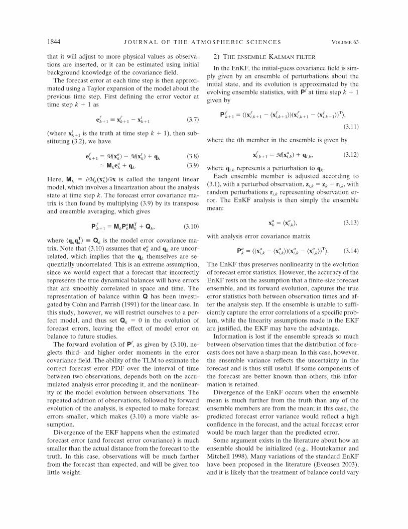
Figure 1 shows two example assimilation runs for the

FIG. 1. Sample analyses of the single time-scale model, for the (left) EKF and (right) EnKF, at twoobservation frequencies, with observations of w (circles) and the same initial perturbation. In all plots,the true state of w (solid) is compared to the analysis (dashed) and, in the EnKF case, the ensemble(gray). The forecast error covariance �(ef

w)2� is shown below the respective plots for each case.

JULY 2006 N E E F E T A L . 1845

single-time scale model, using the EKF (left) and theEnKF (right). Observations of w are taken every timeunit (top row) and every six time units (i.e., roughlyonce during a typical cycle of the slow mode, bottomrow) in each case, with the same truth for all cases.Each plot compares the true state to the assimilatedanalysis, along with the forecast error variance �(e f

w)2�.For the EKF cases in this example, the initial forecasterror covariance matrix is estimated by a diagonal ma-trix,

P0f � �0

2I, �3.19�

with the expectation that the series of analysis steps willadjust P f to a more physical value (the criticality of thisassumption, in terms of balance, is explored more thor-oughly below). An ensemble of N � 20 forecasts is usedfor the EnKF. The examples in Fig. 1 illustrate severalkey properties of Kalman filter assimilation for nonlin-ear, chaotic dynamics.

Good analysis increments are made when growth inthe forecast error covariance for each variable reflectsthe rate at which the forecast is diverging from the truestate. The forecast error grows when the forecast andtrue state diverge, and then decreases sharply when anobservation is made. For the EnKF (Figs. 1b,d), growthin the forecast error variance term for each variablereflects the visible spread in the ensemble.

The accuracy of the analysis, in both schemes, de-creases for �tobs � 6. A difference between the EKFand EnKF also starts to become clear at larger �tobs: the

spread of the ensemble between observations, in theEnKF case, becomes less Gaussian, which means thatTLM-predicted error covariances will become less ac-curate.

Note also that the analyses of w in Fig. 1 depend onthe ability of each Kalman filter to estimate the entirestate (w and � ) from observations of just one compo-nent of it (w). This is the crux of the overall data as-similation problem, and will form the basis of the morespecific problem of balance.

A more quantitative comparison of the two filters isshown in Fig. 2, which shows the analysis error imme-diately following the insertion of each observation, av-eraged over 600 runs, for the EKF (left panel) and theEnKF (right panel), at �tobs � 1–7. For the EnKF case,errors are shown for runs with ensembles of 4 and 10forecasts. Comparison of these two figures reveals thatthe performance of the EnKF is similar to the EKF ifthe forecast ensemble consists of four forecasts, thoughthe analysis error in the EnKF is somewhat reducedwhen the ensemble size is increased to 10 forecasts.Moreover, analysis errors grow in time for all casesshown, except for �tobs � 1 for the EKF, and �tobs � 1and 2 for the 10-forecast EnKF.

d. Balance in the assimilation problem

In light of the single time-scale results, we now askwhether, and under what conditions, the EKF andEnKF evolve forecast error covariances that reflect thedynamical balance in the true state. The degree of bal-

FIG. 2. Comparison of the average state error (over 600 runs) immediately following theanalysis steps with (left) the EKF and (right) the EnKF, for the single time-scale model. Forthe EnKF, we also compare ensemble sizes N � 4 (black) and N � 10 (gray). Observationfrequencies shown are �tobs � 1 (x), 2 (circles), 3 (�), 4 (triangles), 5 (inverted triangles), 6(squares), and 7 (dots). In all runs, the initial true state is randomly generated and then theforecast and observations are generated using (3.15) and (3.16).


ance captured by Pf, for both Kalman filters, will de-pend on each scheme’s treatment of balance in (i) theinitial-guess error covariances, (ii) the evolution of er-ror covariances, and (iii) the repeated adjustment oferror covariances by the Kalman gain.

To examine what it means for error covariances toreflect balance, we define a balanced error covariancematrix as one where the errors in the “slaved” fast vari-ables are dependent on the errors in the slow “master”variables. For a perfectly balanced state with zero freefast motion, the errors in the fast variables will then beentirely functions of the errors in the slow variables.

Defining e fy � y f � yt as the forecast error vector in

terms of the slow variables, the forecast error in termsof mixed time-scale variables can be approximated as aTaylor expansion of (2.7):

exf � x f � xt � Ley

f � nonlinear terms, �3.20�

where L � (�f/�y)|y t is the first derivative of the balancerelationship, evaluated about the slow-manifold fore-cast state at some point in time. The forecast errorcovariances are found by multiplying (3.20) by its trans-pose, and computing the ensemble mean. Truncating(3.20) at the linear term, the forecast error covariancematrix, in terms of the full model state, can be approxi-mated as

Pxf � �ex

f �exf �T� � ��Ley

f ��Leyf �T�

� L�eyf �ey

f �T�LT � LPyf LT, �3.21�

where we have defined

Pyf � �ey

f �eyf �T� �3.22�

as the error covariance matrix in terms of the slow vari-ables only. Since (3.21) is a tangent linear operation, acovariance matrix P f

x that is formulated in this way canbe thought of as tangent to the balance manifold. Thus,(3.21) will hereafter be referred to as a tangent linearbalance transformation, or TLBT, in analogy to theTLM (3.10). As in the TLM, this approximation ne-glects dependence on higher order statistical momentsin the forecast error distribution.

For the exL86 model,

L � �1 0

��2b�Uz

��2�1 � b

�Uz

�w ��Ux

��

�Ux

�w� 0

�2�Uz

��2��Uz

�w� b� �, �3.23�

and is a function of the slow variable state. The accu-racy of (3.21) depends (as in the TLM) on the magni-tude of e f

y, but also on the size of �, and the order ofaccuracy in � to which the balance approximation ismade.

4. Balance in the extended Kalman filter

a. Example

Figure 3 shows four example EKF assimilation ex-periments for the exL86 model, all with the same (bal-anced) true state and initial perturbation. Observationsin all four cases are taken of w, and thus contain bothtime scales. The initial and final values of Imb (for theanalysis) are shown for each case, and the forecast errorvariance �(e f

w)2� is shown underneath each analysis.

The forecasts in Figs. 3a,b are initialized using (2.5)–(2.6), following the initial perturbation, thus reflecting acase where there is a priori knowledge of the absence ofgravity waves. In Figs. 3c,d, the initial forecasts are un-balanced, with initial imbalance due only to initial fore-cast error.

Very frequent observations (�tobs � 1, left column ofplots), are again compared to observations taken on theorder of a typical cycle of the slow mode (�tobs � 6,right column of plots). In all four cases shown, the ini-tial covariance field is estimated by (3.19), where I isnow the 4 � 4 identity matrix.

The primary result of this example is that balance inthe EKF analysis depends largely on observation fre-quency. We note also that very frequent observationsnot only retain balance in a balanced initial forecast(Fig. 3a), but can also establish balance in an unbal-anced initial forecast (Fig. 3c), despite the fact that nobalance information is contained in the initial forecasterror covariances. For �tobs� 6, on the other hand, bal-ance deteriorates after a few observations, and mostinformation from subsequent observations is conse-quently rejected. In these cases, the covariance modelitself takes on a significant fast oscillation, which is notremoved by the addition of observations.

Though this example depends in detail on the par-ticular instabilities and realizations of the random er-rors used, it points out two important factors for bal-ance in the EKF. The first is observation frequency: Forlonger �tobs, the forecast drifts more from the truth,resulting in a larger analysis increment, which in turnamplifies any misestimations of the forecast errors and,more importantly, of the balance relationship in theerror covariances. The second factor is the initializationof the covariance model, via P f

0. Since the forecast errorcovariances in Figs. 3b,d clearly do not adjust to reflectthe balance relationship, it is worth investigating to

JULY 2006 N E E F E T A L . 1847

what extent the covariance model may be improved byproviding it with an initial knowledge of balance, as in(3.21), and the extent to which this information is re-tained as the assimilation progresses.

b. Balance in the EKF covariance model

How does the EKF covariance model capture thebalance relationship? This problem has three generalcomponents.

1) INITIAL ESTIMATE OF P f

Instead of specifying an initial time error covariancematrix using (3.19)—that is, with no correlations be-tween variables—one might instead initialize Pf usingthe TLBT (3.21), or some approximation to it. The ac-curacy of such an initialization depends on how well thebalance relation is known, and the validity of the lin-earization. For small �, the higher order balance terms

become less important, and the drift of an initializedstate from the slow manifold becomes slower. The non-linear terms in f also become less important for small �.Thus, the usefulness of balance-initializing Pf

0 dependson the smallness of �.

2) TLM EVOLUTION OF P f

It is not clear whether a forecast error covariancematrix initialized using the TLBT will remain tangentto the slow manifold as it is evolved in the TLM (3.10).This question can be examined by comparing the TLMevolution of the error vector (3.9) to the true error(3.8). If, at time step k, both the forecast and the truestate are balanced, such that

xkt � f�yk

t � �4.1�

xka � f�yk

a�, �4.2�

and if the model error is zero, then the true error at thenext time step will be given by

FIG. 3. Four sample EKF assimilations for the full (multiple time scale) exL86 model. For each case,the truth (black) and analysis (gray) of w are shown, along with the observations (circles). Underneatheach plot is shown the forecast error variance for w. (a) Balanced initial forecast, with �tobs � 1. (b)Balanced initial forecast, with �tobs � 6. (c) Unbalanced initial forecast, with �tobs � 1. (d) Unbalancedinitial forecast, with �tobs � 6. The initial perturbation is �x � (0.450, �0.800, �0.465, 0.725)T. Initial andfinal values of Imb are shown on each plot.


ex,k�1f � M �f�yk

a� � M �f�ykt � . �4.3�

If the forecast model evolves a balanced state to pro-duce a balanced state, then

ex,k�1f � f�yk�1

f � � f�yk�1t �. �4.4�

In contrast, if the forecast errors at time step k arebalanced according to (3.21), then the forecast errors atthe next time step are given by

ex,k�1f � MkLkey,k

a . �4.5�

They remain tangent to the slow manifold if

MkLkey,ka � Lk�1ey,k�1

f . �4.6�

3) ANALYSIS STEP

For the standard EKF, use of the TLM is justified ifthe information brought in from observations in (3.6) isable to keep the evolving covariance model close to thetrue error statistics. Extending this to balance, we ex-pect that the assimilation of observations can also makethe degree of balance represented in the covariancemodel more accurate.

If the forecast error covariance matrix (in terms ofmixed variables) is balanced—that is, if Pf

x,k � LkPfy,kLT

k—then the gain matrix becomes

Kx,k � Px,kf Hk

T�HkPx,kf Hk

T � R��1 �4.7�

�LkPy,kf Lk

THkT�HkLkPy,k

f LkTHk

T � R��1 �4.8�

�LkPy,kf Gk

T�GkPy,kf Gk

T � R��1 �4.9�

� LkKy,k, �4.10�

where we have defined Ky,k as the gain matrix in termsof the slow variables, and Gk � HkLk as a generalizedobservation operator. Note that Gk selects only theslow-manifold projection of the observed variable, andKx,k, consequently, includes the TLBT.

The analysis error covariance matrix is then given by

Px,ka � �I � Kx,kHk�LkPy,k

f LkT �4.11�

�Lk�Py,kf � Lk

� 1Kx,kHkLkPy,kf �Lk

T �4.12�

�Lk�I � Ky,kGk�Py,kf Lk

T �4.13�

�LkPy,ka Lk

T. �4.14�

Since Pax,k can be written as LkPa

y,kLTk , it is still tangent to

the slow manifold. Thus, (3.6) retains the TLBT, whilestill being reduced to include information from the ob-servations.

The above transformations are equivalent to thosederived by Cohn and Parrish (1991) for the linear case.

For the present (nonlinear) case, balanced forecast er-rors in the EKF rely on four assumptions. First, theTLM must be a valid approximation over �tobs, whichdepends on the size of the forecast error. Second, theTLBT must be a valid approximation. This also de-pends on the size of the forecast error, as well as on thesize of � and the order of accuracy of the slaving rela-tions. Third, the initial truth and initial forecast must bebalanced. Fourth, the model evolution must preservebalance. In the exL86 model, this is only true to theorder in � to which the model was initialized.

Therefore, while it makes sense to initialize Pf0 using

the TLBT, it is not obvious that such an initializationwill ensure a balanced assimilation.

c. Numerical evaluation of the EKF

Figure 4 shows the average, over 600 assimilationruns, of the fast and slow analysis errors [(3.17)–(3.18)],immediately following each analysis, as a function ofobservation time. The observed variable in all runs isw. Both figures compare runs where Pf

0 is initializedusing the TLBT, to ones where Pf

0 is chosen as a diago-nal matrix (3.19). Also shown are runs where it is as-sumed that the balance relations are not known, but areguessed to be functions that are proportional to �, suchthat the tangent error covariances are approximated as

P0f � �0

2�1 0 � 0

0 1 � 1

� � �2 0

0 1 0 1 . �4.15�

For each case, three observation frequencies (�tobs � 2,4, and 6) are shown.

The first thing to note is that the analysis of the slowmode is unstable for �tobs � 2; the average slow analysiserrors all grow as the assimilation progresses. Averagefast error does not depend strongly on observation fre-quency, and in fact tends to level off as the assimilationprogresses. This indicates that the failure of the EKF atthese observation frequencies is due to filter diver-gence, which can be verified by comparing the forecasterrors and true errors for these cases. Forecast errorsbecome much smaller than the true errors (not shown),and observations consequently have no impact on theforecast. For the chaotic slow mode, this means that thedistance between truth and analysis will then grow intime, whereas the spurious fast wave, and thus fast er-ror, neither decays nor grows.

However, initializing Pf0 with a knowledge of the bal-

ance relationship clearly decreases the overall fast er-

JULY 2006 N E E F E T A L . 1849

ror. When Pf0 is initialized without correlations between

variables, the average fast error immediately exceedsthe magnitude of the slaved mode in the true state(2.5)–(2.6), which is O(�). If Pf is initialized with theTLBT, the average fast error (for the assimilation pe-riods considered) stays below the magnitude of theslaved fast mode, even for �tobs � 6. Even an educatedguess at balanced error covariances (4.15) improves thefast error substantially. While the growth of fast error ineach case is similar, the overall imbalance is smaller ifPf

0 is properly initialized, simply because the spuriousimbalance induced by the first few analysis steps is less.

We note also that the average analysis error for theslow mode does not depend significantly on the initial-ization of Pf

0. This means that an EKF initialized with(3.19) may still succeed in terms of the slow mode, evenwhile the analysis contains a spurious fast mode.

Figure 5 examines the effectiveness of initializing Pf0

using the TLBT, as a function of �. It shows the fasterror following the single insertion of an observation att � 4 (for 600 different assimilation runs) with varyingvalues of �, and with Pf

0 initialized either using (3.19) or(3.21). A curve corresponding to �2 is added to Fig. 5 inorder to emphasize the asymptotic nature of the TLBT.For � smaller than about 0.3, the initialization of Pf withthe TLBT tends to yield an analysis with smaller fasterror, while as � increases, the initialization of Pf

0 nolonger makes a difference in the fast error. This makessense, since the separation of fast and slow modes be-comes asymptotically less well defined as � → 1.

d. EKF with a balance constraint

A balance constraint can be incorporated into theEKF, by performing the analysis step in terms of theprojection of the model state onto the slow variablesy � (�, w)T only. Starting from a mixed time-scaleforecast xf

k, the projection onto the slow manifold isgiven by

ykf � Fxk

f �4.16�

Pyf � FPx

f FT. �4.17�

FIG. 5. Fast error immediately following the insertion of anobservation at t � 4, for 600 randomly initialized runs (as in Fig.4), as a function of �. The x’s are runs where Pf

0 is initialized usingthe balance approximation (3.21), and circles where Pf

0 is initializedas a diagonal matrix (3.19). The �2 curve is also shown (solid line).

FIG. 4. Comparison of the average (left) fast and (right) slow analysis error, following eachanalysis step, between three ways of initializing the error covariance matrix: either using thebalance approximation [(3.21), black], or by initializing Pf

0 as a diagonal matrix [(3.19), gray],or by guessing at a balance relation [(4.15), dashed]. Three observation frequencies are com-pared for each case: �tobs � 2 (circles), 4 (triangles), and 6 (squares). The average is over 600assimilation experiments.


It is followed by the analysis step:

yka � yk

f � Ky,k�zk � Hkf�ykf � , �4.18�

where Ky,k � P fy,kGT

k(GkP fy,kGT

k � R)�1. Note that Ky,k

uses the TLBT in order to select the slow-manifoldprojection of the observation error. The analysis interms of the full model state can then be computed bymapping the slow state back to a balanced mixed-variable state, using (2.7).

Alternatively, one could map the gain matrix back tothe mixed-variable state, and update the mixed time-scale state as

xka � xk

f � Kx,k�zk � Hkxkf � xk

f � LkKy,k�zk � Hkxkf ,

� xkf � Lkyk, �4.19�

where �yk � yak � y f

k � Ky,k(zk � Hkx fk) is the analysis

increment on the slow manifold. However, this requiresan additional use of the TLBT.

A comparison between these two modified analysissteps and the regular EKF is shown as before, in theaverage fast error (Fig. 6) immediately following eachanalysis step, for observation frequencies �tobs � 2, 4,and 6. For increasing �tobs, the modified schemes offera substantial improvement over the TLBT–EKF, withthe direct-transformation analysis [(4.18)] yielding onaverage more balanced analyses than the indirectanalysis [(4.19)]. This is not surprising because the in-direct transformation uses an additional approxima-tion. However, for frequent observations, the indirectrelationship may be sufficient.

5. Balance in the ensemble Kalman filter

The single time-scale example in section 3 showedthat the EnKF, by preserving the nonlinearity of theevolving error distribution, may be preferable to theEKF. The EnKF is a (weakly nonlinear) combinationof model states (Evensen 2003), which suggests that theEnKF analysis might naturally be more balanced. Also,the averaging nature of the analysis step in itself impliesa kind of balancing. A balanced analysis state is still notguaranteed, however, as long as fast waves are allowedin the individual ensemble members.

How can the EnKF covariance model capture bal-ance? If Pf is given by an ensemble of balanced fore-casts, no TLBT approximation is required. Balancedperturbations for the exL86 model can be generated bytransforming the central forecast to normal modes,adding random perturbations to � f and wf, and thentransforming back to mixed variables using (2.7). [Inrealistic applications, this step is a bit more compli-cated, but similar. For example, one can randomly per-turb streamfunction, and then derive wind, tempera-ture, and pressure perturbations following some bal-ance assumption (see, e.g., Mitchell et al. 2002). In lieuof an explicit slow manifold initialization, one mightalso integrate the ensemble forward while filtering outfast waves with, say, a digital filter (Evensen 1997).]

Whether or not the forward evolution of such anensemble and the subsequent ensemble analysis indeedyields a balanced analysis, however, depends on threeassumptions, which in turn depend on observation fre-quency and the size of the forecast ensemble: First, thatthe evolving N-member forecast ensemble sufficientlyrepresents the full statistics of the true system, includingbalance; second, that the analysis step does not destroythe ensemble’s representativeness; and, third, that theensemble analysis step (3.13) yields a balanced state.

a. Example

Figure 7 shows two sample EnKF assimilation runs,with observations of w, and all other assimilation pa-rameters as in the EKF example (section 4). The ob-servation frequency is �tobs � 1 in Fig. 7a, and �tobs �6 in Fig. 7b. To illustrate more clearly how the forecastensemble captures the balance relationship, the analy-ses of x are shown for each case along with the analysesof w. In both cases shown, the ensemble size is N � 10forecasts.

For �tobs � 1, the ensemble collapses toward a singleforecast which is often indistinguishable from the truestate, whereas for �tobs � 6, the ensemble diverges sig-nificantly between observations—though, in both cases,

FIG. 6. As in Fig. 4, but now comparing the two balance-constraint modifications to the EKF: either by (black, solid) di-rectly balancing the analysis via (4.18) followed by (2.7), or by(gray, solid) indirectly mapping the analysis increment as in(4.19). These modified schemes are compared to the regular EKF(black, dashed), where Pf

0 is initialized using the tangent approxi-mation (3.21). As in previous figures, observation frequenciesshown are �tobs � 2 (circles), 4 (triangles), and 6 (squares).

JULY 2006 N E E F E T A L . 1851

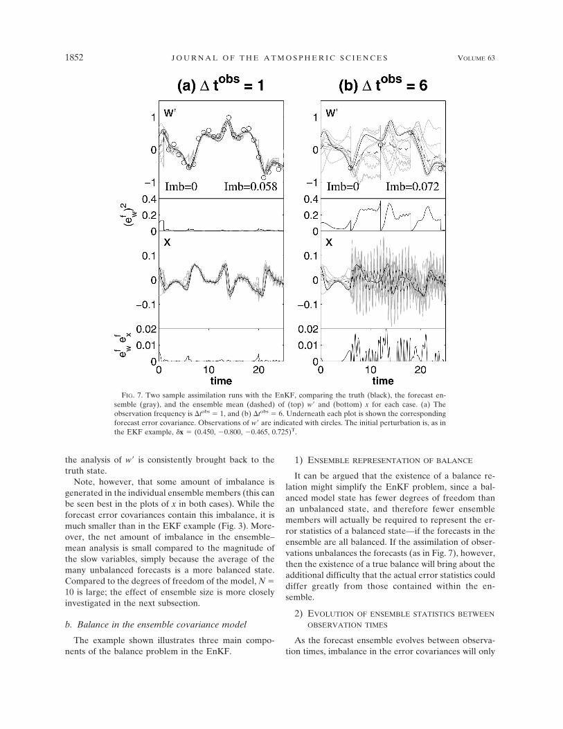
the analysis of w is consistently brought back to thetruth state.

Note, however, that some amount of imbalance isgenerated in the individual ensemble members (this canbe seen best in the plots of x in both cases). While theforecast error covariances contain this imbalance, it ismuch smaller than in the EKF example (Fig. 3). More-over, the net amount of imbalance in the ensemble–mean analysis is small compared to the magnitude ofthe slow variables, simply because the average of themany unbalanced forecasts is a more balanced state.Compared to the degrees of freedom of the model, N �10 is large; the effect of ensemble size is more closelyinvestigated in the next subsection.

b. Balance in the ensemble covariance model

The example shown illustrates three main compo-nents of the balance problem in the EnKF.

1) ENSEMBLE REPRESENTATION OF BALANCE

It can be argued that the existence of a balance re-lation might simplify the EnKF problem, since a bal-anced model state has fewer degrees of freedom thanan unbalanced state, and therefore fewer ensemblemembers will actually be required to represent the er-ror statistics of a balanced state—if the forecasts in theensemble are all balanced. If the assimilation of obser-vations unbalances the forecasts (as in Fig. 7), however,then the existence of a true balance will bring about theadditional difficulty that the actual error statistics coulddiffer greatly from those contained within the en-semble.

2) EVOLUTION OF ENSEMBLE STATISTICS BETWEEN

OBSERVATION TIMES

As the forecast ensemble evolves between observa-tion times, imbalance in the error covariances will only

FIG. 7. Two sample assimilation runs with the EnKF, comparing the truth (black), the forecast en-semble (gray), and the ensemble mean (dashed) of (top) w and (bottom) x for each case. (a) Theobservation frequency is �tobs � 1, and (b) �tobs � 6. Underneath each plot is shown the correspondingforecast error covariance. Observations of w are indicated with circles. The initial perturbation is, as inthe EKF example, �x � (0.450, �0.800, �0.465, 0.725)T.


grow as much as the mean imbalance in the ensemble(as opposed to the unbounded growth that would hap-pen with the TLM evolution of errors). Even if theensemble spread becomes saturated in the slow mode,it could still contain information about the (slaved) fastmode (though this is not shown in Fig. 7).

3) ENSEMBLE ANALYSIS STEP

It was shown above that even an ensemble of bal-anced forecasts will to some extent result in individualanalyses that are unbalanced. The amount of imbalanceremaining in the ensemble mean will then depend onthe magnitude and relative phases of the fast motion inindividual analyses. It may thus be argued that, formodels with a spatial dimension and a spectrum of pos-sible gravity waves, spurious imbalance in individualensemble members will easily disappear in the en-semble average. The results of Houtekamer and Mitch-ell (1998) suggest, however, that spurious imbalance inthe ensemble mean analysis is difficult to avoid for re-alistic ensemble sizes.

It is also important to note that the ensemble candevelop a very small variance (reflecting high confi-dence in the forecast) around a significantly unbalancedmean forecast. Thus, a form of filter divergence, interms of balance, can happen, wherein the forecast en-semble has a very narrow distribution, but predicts thewrong type of motion—in this case, a gravity wave.Here we note that filter divergence is related to thedetails of how the ensemble is generated and how theanalysis step is carried out. While we are aware of theknown caveats of the Burgers et al. (1998) and

Houtekamer and Mitchell (1998) formulation of theEnKF, it is used here as a first step to illustrating thebalance properties of the EnKF.

The example in Fig. 7 shows that, while the EnKFmay be advantageous for at least two reasons (by al-lowing for the nonlinear evolution of error statistics,and because spurious imbalance may be filtered out inthe ensemble mean), even if the assimilation is begunwith an ensemble of balanced forecasts, the repeatedadjustment of these forecasts may not yield an analysisthat is balanced.

c. Numerical evaluation of the EnKF

A comparison of the EnKF and EKF is shown in Fig.8, again comparing the mean (over 600 runs) fast andslow errors, for observation frequencies of �tobs � 2, 4,6. In these experiments, observations of w were ran-domly alternated with observations of �. These experi-ments thus simulate a case in which we have a variety ofobservations, with some of the slow mode only. EnKFcases with N � 4 and N � 10 forecasts are compared tothe EKF case where P f

0 is initialized using the TLBT.The performance of the EnKF is comparable to that

of the TLBT-initialized EKF for the first few observa-tions, but has a slower growth of analysis error as theassimilation progresses. The EnKF is also, on average,more accurate for longer �tobs: At t � 10, the fast errorfor the EnKF, for both ensemble sizes shown, is con-sistently smaller than the EKF fast error at correspond-ing observation frequencies (except at �tobs � 2). TheEnKF slow error levels off for both ensemble sizes,whereas the corresponding EKF slow error grows in time.

FIG. 8. Comparison of the average (left) fast and (right) slow analysis error, now comparingthe EKF (gray) to the EnKF, for ensembles of N � 4 forecasts (black, solid) and N � 10forecasts (black, dashed). For the EKF, Pf

0 is initialized using the TLBT (3.21). In theseexperiments, observations of w were randomly alternated with observations of �.

JULY 2006 N E E F E T A L . 1853

It is also interesting to note that increasing observa-tion frequency improves the EnKF estimate for theslow mode, but actually seems to worsen the estimate ofthe slaved fast mode. This is a robust result for similarexperiments with different ensemble sizes, and is ex-plainable: more frequent forcing of the forecasts in theensemble means that there are more chances to excitespurious fast motion in individual forecasts and, conse-quently, balance in the ensemble covariance model de-teriorates earlier. If observations are less frequent, thegravity wave in each ensemble member, and hence thenet imbalance in the covariance model, cannot grow asquickly, and the overall analysis is consequently morebalanced.

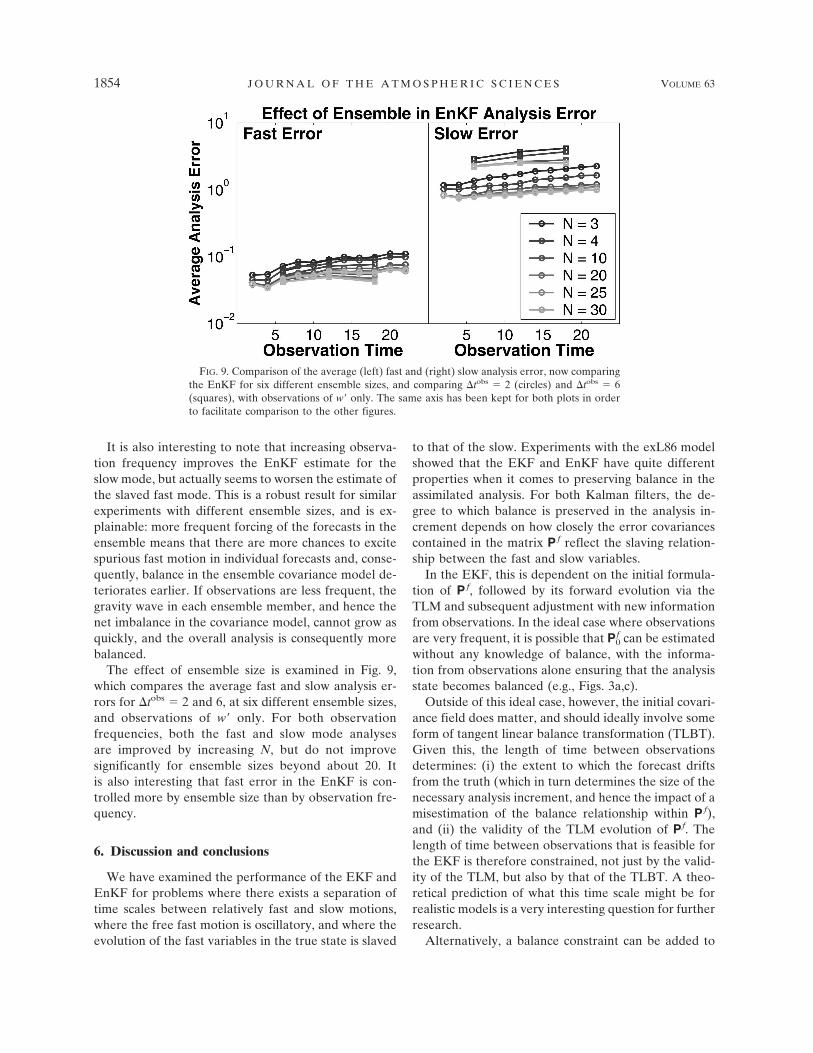
The effect of ensemble size is examined in Fig. 9,which compares the average fast and slow analysis er-rors for �tobs � 2 and 6, at six different ensemble sizes,and observations of w only. For both observationfrequencies, both the fast and slow mode analysesare improved by increasing N, but do not improvesignificantly for ensemble sizes beyond about 20. Itis also interesting that fast error in the EnKF is con-trolled more by ensemble size than by observation fre-quency.

6. Discussion and conclusions

We have examined the performance of the EKF andEnKF for problems where there exists a separation oftime scales between relatively fast and slow motions,where the free fast motion is oscillatory, and where theevolution of the fast variables in the true state is slaved

to that of the slow. Experiments with the exL86 modelshowed that the EKF and EnKF have quite differentproperties when it comes to preserving balance in theassimilated analysis. For both Kalman filters, the de-gree to which balance is preserved in the analysis in-crement depends on how closely the error covariancescontained in the matrix P f reflect the slaving relation-ship between the fast and slow variables.

In the EKF, this is dependent on the initial formula-tion of P f, followed by its forward evolution via theTLM and subsequent adjustment with new informationfrom observations. In the ideal case where observationsare very frequent, it is possible that Pf

0 can be estimatedwithout any knowledge of balance, with the informa-tion from observations alone ensuring that the analysisstate becomes balanced (e.g., Figs. 3a,c).

Outside of this ideal case, however, the initial covari-ance field does matter, and should ideally involve someform of tangent linear balance transformation (TLBT).Given this, the length of time between observationsdetermines: (i) the extent to which the forecast driftsfrom the truth (which in turn determines the size of thenecessary analysis increment, and hence the impact of amisestimation of the balance relationship within P f),and (ii) the validity of the TLM evolution of Pf. Thelength of time between observations that is feasible forthe EKF is therefore constrained, not just by the valid-ity of the TLM, but also by that of the TLBT. A theo-retical prediction of what this time scale might be forrealistic models is a very interesting question for furtherresearch.

Alternatively, a balance constraint can be added to

FIG. 9. Comparison of the average (left) fast and (right) slow analysis error, now comparingthe EnKF for six different ensemble sizes, and comparing �tobs � 2 (circles) and �tobs � 6(squares), with observations of w only. The same axis has been kept for both plots in orderto facilitate comparison to the other figures.


the EKF algorithm. This can be done by projecting themodel state onto the slow manifold, performing theanalysis in terms of the slow variables only, and thenusing the slaving relationship to compute the analysis interms of mixed variables. Numerical experimentsshowed that such a constraint can significantly improvethe EKF analysis at observation frequencies where bal-ance is otherwise lost, but relies upon accurate knowl-edge of the balance relationship.

The EnKF has two possible advantages for balance:First, it retains the balance relationship to the extentthat ensemble members themselves are balanced, be-cause the forecasts in the ensemble use the full nonlin-ear model and the gravity wave is therefore bounded.Secondly, the ensemble-averaging in the analysis stepmeans that a spurious gravity wave in a single forecastis compared to every other forecast, so that the result-ing analysis has less net imbalance. Note, however, thatthis assumes that the ensemble is sufficiently phasemixed. If several ensemble members contain the samegravity wave, this wave will not average out (this can beseen in Fig. 7).

The accuracy of the EnKF is nonetheless limited byensemble size. Numerical experiments showed that,while the knowledge of a balance relationship reducesthe dimension of the problem, enough ensemble mem-bers are still required to capture, within the covariancematrix, the fact that the fast mode is slaved to the slow.For the exL86 model, the best-possible balanced analy-sis required an ensemble of at least 20 forecasts, whichis much larger than the degrees of freedom of the prob-lem (which is four).

A numerical comparison of the EKF and EnKF (Fig.8) showed that the two schemes seem to perform simi-larly well, in terms of balance, when the initial covari-ance model in the EKF is computed using a TLBT, andwhen the ensemble in the EnKF is large enough tocapture the slaving of the fast motion. The consequenceof the EnKF’s two additional properties is that (i)growth of imbalance in the analysis, as the assimilationprogresses, is slower in the EnKF, and (ii) the EnKFallows for longer time intervals between observationswithout a great loss of balance.

This stability of the EnKF reflects the stability ofgravity waves in the exL86 model; whereas, in contrast,gravity waves can grow in the TLM. The way in whichgravity waves grow in the TLM has been illustratednumerically but not yet investigated analytically. Fu-ture work will further investigate the development ofimbalance in the TLM.

Another property to note about the EnKF is thatobserving too frequently can overforce the ensemble,and actually cause greater imbalance, if there are not

enough other gravity waves in the ensemble to elimi-nate the spurious gravity wave (via phase mixing) in theensemble mean.

This study is intended as a complement to similarstudies involving larger, more complicated models, suchas Mitchell et al. (2002). We have highlighted, in asimple context, several key points of the balance prob-lem in the still-evolving field of 4D data assimilation.This extends beyond the problem of spurious gravitywaves, to any problem where there is a time scale ofinterest, and a comparatively fast, unobserved scale(e.g., Lorenz 1995). Our results suggest several inter-esting points for further research:

More degrees of freedom. An analysis similar to thisone could be carried out with a model that is morecomplex than the exL86 model, yet still simpleenough to retain the transparency of this analysis.A model that admits more than one gravity wavefrequency, or more spatial degrees of freedom,would make it possible to address the effects of,say, geostrophic adjustment or localization of errorcovariances.

Chaotic (non–gravity wave) fast mode. A model inwhich the fast mode is chaotic (in which case slavingis impossible), such as the two time-scale model ofLorenz (1995), is another interesting context for ex-amining assimilation for multiple time scales, andcould address problems of mesoscale and convective-scale assimilation (e.g., Snyder and Zhang 2003).

Variations on the standard algorithms. Many varia-tions of the EKF and EnKF have been proposed inrecent years, with the intent of either increasingcost-efficiency, or of freeing the KF from some ofthe assumptions on which it rests. These are wellsummarized by Evensen (2003).

Square root filters (SRF) compute analysis en-sembles deterministically from the analysis covari-ance matrix given by (3.6), which reduces samplingerror, and thus helps prevent filter divergence(Tippett et al. 2003, and references therein). Thismight prevent undesirable phase locking such aswe see in Fig. 7. The accuracy and possible differ-ences between the various incarnations of SRFsschemes, with respect to balance, is, to our knowl-edge, still to be investigated.

Schemes that rely on fewer linearity assumptionsmay also handle balance dynamics more accu-rately, since (as shown in this study) balance in theassimilation often fails because of faulty assump-tions of linearity. A particle filter (Anderson andAnderson 1999; Pham 2001), for example, departsfrom the standard KF linear analysis step (3.1), and

JULY 2006 N E E F E T A L . 1855

may thus skirt some of the problems cited in ourstudy, such as gravity wave explosions in the EKF,or undesirable phase-locking of the ensemble.

Modifications to the EnKF that are intended toimprove cost-efficiency might turn out to be natu-rally beneficial for balance, because such schemestake advantage of the low-dimensionality of themodel attractor, and, in the real atmosphere, theslow manifold is itself a lower-dimensional attrac-tor. Examples of such schemes are the singularevolutive interpolated Kalman (SEIK) filter ofPham (2001), and schemes in which the ensembleis constrained by bred vectors (e.g., Toth and Kal-nay 1997) or singular vectors (e.g., Ehrendorferand Tribbia 1997).

Comparison to 4DVAR. This analysis could be ex-tended from the Kalman filter to 4DVAR assimi-lation. While 4DVAR also makes use of a TLM, itsanalysis cycle, and the formulation of the forecasterror covariance field, is quite different, and it isunclear how these differences change the treat-ment of nonlinear balance.

Unclear time-scale separation. We have not yet exam-ined cases where two different motions are admit-ted, but not well-separated in time scale. In theTropics, for example, Žagar et al. (2004) proposean approach whereby capturing balance means in-terpreting the observed field as the right combina-tion of the different types of tropical waves that arepresent. In the exL86 model, this problem can beapproached by letting � → 1.

Unbalanced truth state. It also remains to examinehow the nonlinear KFs perform in the case whereboth fast and slow motion is present in the true state,or rather, where the fast waves carry a significantamount of energy, such as in the mesosphere.

Effect of model error. This study dealt with a veryspecialized situation where both the model dynam-ics and the balance relationship are perfectlyknown. Since this is far from true in realistic cases,the effect of model error formulation on balanceneeds to be investigated. Even in the perfect modellimit, the addition of a model error term in theEKF forecast error evolution (3.10) may stabilizethe analysis step, and prevent observations fromshocking the system into highly unbalanced states,as in Fig. 3b. Similarly, adding stochastic errors tothe ensemble in the EnKF (3.12) could prevent thephase-locking of the ensemble around a spuriousgravity wave.

Acknowledgments. This research was supported inpart by the Modelling of Global Chemistry for Climate

project, with support from the Natural Sciences andEngineering Research Council, the Meteorological Ser-vice of Canada through its Climate Research Network,the Canadian Space Agency, and the Canadian Foun-dation for Climate and Atmospheric Sciences. LN hasalso been supported by a University of Toronto OpenFellowship and a University of Toronto Blythe Fellow-ship. The authors thank Philippe Courtier and JeanCôté for helpful suggestions during the development ofthis work, and Peter Houtekamer, Jeff Kepert, and twoanonymous reviewers, for comments and suggestionson the manuscript.

APPENDIX

Derivation of the exL86 Model

The following is a summary derivation of the exL86model, tracing the development of this simple systemthrough four papers: Lorenz (1980, 1986), Bokhove andShepherd (1996), and WS00.

In Lorenz (1980), the f-plane shallow water equa-tions are nondimensionalized and then simplified byexpanding vorticity, divergence, and height as an inter-acting resonant wave triad. This yields a system of nineequations that describe the evolution of the vorticity,divergence, and height of three interacting waves.These amplitudes are then transformed into normalmodes, corresponding to potential vorticity, diver-gence, and geostrophic imbalance. In Lorenz (1986),the latter two variables are eliminated for two of thethree waves, which leaves two geostrophic vorticitymodes, and a third wave which admits both vorticalmotion and a gravity wave. Here, U and V are thevorticity amplitudes of the two truncated waves; andW, X, and Z are the potential vorticity, divergence,and geostrophic imbalance of the third wave, respec-tively. The equations that describe their evolution aregiven by

dU

dT� �VW � bVZ �A.1�

dV

dT� UW � bUZ �A.2�

dW

dT� �UV �A.3�

dX

dT� �Z �A.4�

dZ

dT� bUV � X. �A.5�


These equations describe a nonlinearly interacting vor-ticity triad (U, V, and W), coupled to an inertia-gravitywave (X and Z). The parameter b is the rotationalFroude number of the third wave.

Bokhove and Shepherd (1996) emphasize the time-scale separation between the nonlinear vortical modeand the gravity wave by scaling the variable amplitudesU � �u, V � ��, W � �w, X � �x, Z � �z, and scalingtime T � t/�. The scaled system is

du

dt� �w � bz �A.6�

d

dt� uw � buz �A.7�

dw

dt� �u �A.8�

dx

dt� �

z

��A.9�

dz

dt� bu �

x

�. �A.10�

For � � 1, x and z vary on a time scale that is fastcompared to the evolution of u, �, and w. From thedimensions of the original equations, it can be shownthat �, which defines the inverse of the ratio betweenthe advective time scale (corresponding to t) and that ofthe inertia-gravity wave, is given by � � RF/�R2 � F2,where R is the Rossby number and F the Froude num-ber.

This system is further simplified by noting the invari-ant C � u2 � �2, and defining u � �C cos�,� � �C sin�, and � � � � �bx. This yields thefollowing four-variable system:

d�

dt� w �A.11�

dw

dt� �

C

2sin�2� � 2�bx� �A.12�

dx

dt� �

z

��A.13�

dz

dt�

x

��

bC

2sin�2� � 2�bx�. �A.14�

Bokhove and Shepherd (1996) showed that the vorticalmode in (A.11)–(A.14) has periodic solutions for mostinitial conditions. To make the evolution of � and wsufficiently chaotic, WS00 let the parameter C vary intime as C(t) � a0 � a1 cost.

Since the present study focuses on the treatment ofthe given time-scale separation in the Kalman filter,

and since observed quantities are not clearly separatedslow or fast variables, it makes sense to transform w andz in the above system back to mixed variables. This issimply done by defining w � w � bz and z � z � bw,which yields the following system:

d�

dt� w� � bz� �A.15�

dw�

dt� �

C

2sin2�� bx� �

�2b

�x �A.16�

dx

dt�

bw� � z�

��A.17�

dz�

dt�

�2x

�, �A.18�

where � � (1 � b2)�(1/2). In this system, � describes the(geostrophic) vorticity of modes 1 and 2, and w, x, andz the (nongeostrophic) vorticity, divergence, andheight, respectively, of mode 3.

REFERENCES

Anderson, J. L., and S. L. Anderson, 1999: A Monte Carlo imple-mentation of the nonlinear filtering problem to produce en-semble assimilations and forecasts. Mon. Wea. Rev., 127,2741–2758.

Bokhove, O., and T. G. Shepherd, 1996: On Hamiltonian bal-anced dynamics and the slowest invariant manifold. J. Atmos.Sci., 53, 276–297.

Burgers, G., P. J. van Leeuwen, and G. Evensen, 1998: Analysisscheme in the ensemble Kalman filter. Mon. Wea. Rev., 126,1719–1724.

Cohn, S. E., and S. F. Parrish, 1991: The behavior of forecast errorcovariances for a Kalman filter in two dimensions. Mon. Wea.Rev., 119, 1757–1785.

Courtier, P., and O. Talagrand, 1990: Variational assimilation ofmeteorological observations with the direct and adjoint shal-low-water equations. Tellus, 42A, 531–549.

Daley, R., 1991: Atmospheric Data Analysis. Cambridge Univer-sity Press, 457 pp.

——, and K. Puri, 1980: Four-dimensional data assimilation andthe slow manifold. Mon. Wea. Rev., 108, 85–99.

Ehrendorfer, M., and J. J. Tribbia, 1997: Optimal prediction offorecast error covariances through singular vectors. J. Atmos.Sci., 54, 286–313.

Evensen, G., 1994: Sequential data assimilation with a nonlinearquasigeostrophic model using Monte Carlo methods to fore-cast error statistics. J. Geophys. Res., 99, 10 143–10 162.

——, 1997: Advanced data assimilation for strongly nonlinear dy-namics. Mon. Wea. Rev., 125, 1342–1354.

——, 2003: The ensemble Kalman filter: Theoretical formulationand practical implementation. Ocean Dyn., 53, 343–367.

Gauthier, P., and J.-N. Thépaut, 2001: Impact of the digital filteras a weak constraint in the preoperational 4DVAR assimila-tion system of Metéo-France. Mon. Wea. Rev., 129, 2089–2102.

Ghil, M., S. Cohn, J. Tavantzis, K. Bube, and E. Isaacson, 1981:Applications of estimation theory to numerical weather pre-

JULY 2006 N E E F E T A L . 1857

diction. Dynamic Meteorology: Data Assimilation Methods,L. Bengtsson, M. Ghil and E. Källén, Eds., Springer-Verlag,139–224.

Houtekamer, P. L., and H. L. Mitchell, 1998: Data assimilationsusing an ensemble Kalman filter technique. Mon. Wea. Rev.,126, 796–811.

Kalman, R. E., 1960: A new approach to linear filtering and pre-diction problems. J. Basic Eng., 82, 35–45.

——, and R. S. Bucy, 1961: New results in linear filtering andprediction theory. J. Basic Eng., 83, 95–108.

Lorenz, E. N., 1963: Deterministic non-periodic flow. J. Atmos.Sci., 20, 130–141.

——, 1980: Attractor sets and quasi-geostrophic equilibrium. J.Atmos. Sci., 37, 1685–1699.

——, 1986: On the existence of a slow manifold. J. Atmos. Sci., 43,1547–1557.

——, 1995: Predictability—A problem partly solved. Proc. Semi-nar on Predictability, Reading, United Kingdom, ECMWF,1–18.

Miller, R. N., M. Ghil, and F. Gauthiez, 1994: Advanced dataassimilation for strongly nonlinear dynamical systems. J. At-mos. Sci., 51, 1037–1056.

Mitchell, H. L., P. L. Houtekamer, and G. Pellerin, 2002: En-semble size, balance, and model-error representation in anensemble Kalman filter. Mon. Wea. Rev., 130, 2791–2808.

Pham, D. T., 2001: Stochastic methods for sequential data assimi-

lation in strongly nonlinear systems. Mon. Wea. Rev., 129,1194–1207.

Polavarapu, S., M. Tanguay, and L. Fillion, 2000: Four-dimen-sional variational data assimilation with digital filter initial-ization. Mon. Wea. Rev., 128, 2491–2510.

Snyder, C., and F. Zhang, 2003: Assimilation of simulated radarobservations with an ensemble Kalman filter. Mon. Wea.Rev., 131, 1663–1677.

Tanguay, M., P. Bartello, and P. Gauthier, 1995: Four-dimension-al data assimilation with a wide range of scales. Tellus, 47A,974–997.

Thépaut, J.-N., and P. Courtier, 1991: Four-dimensional data as-similation using the adjoint of a multilevel primitive equationmodel. Quart. J. Roy. Meteor. Soc., 117, 1225–1254.

Tippett, M. K., J. L. Anderson, C. H. Bishop, T. M. Hamill, andJ. S. Whitaker, 2003: Ensemble square root filters. Mon. Wea.Rev., 131, 1485–1490.

Toth, Z., and E. Kalnay, 1997: Ensemble forecasting at NCEP andthe breeding method. Mon. Wea. Rev., 125, 3297–3319.

Wirosoetisno, D., and T. G. Shepherd, 2000: Averaging, slavingand balanced dynamics in a simple atmospheric model.Physica D, 141, 37–53.

Žagar, N., N. Gustafsson, and E. Källén, 2004: Variational dataassimilation in the tropics: The impact of a background-errorconstraint. Quart. J. Roy. Meteor. Soc., 130, 103–125.


Documents

Four-dimensional data assimilation and balanced dynamics