arX

iv:0

710.

1444

v3 [

astr

o-ph

] 2

9 M

ar 2

008

Detecting Life-bearing Extra-solar Planets with Space Telescopes

Revised version

Steven V. W. Beckwith1,2,3

University of California, 1111 Franklin St., Oakland, CA 94607-5200, USA

steven.beckwith@ucop.edu

ABSTRACT

One of the promising methods to search for life on extra-solar planets (exoplanets) is todetect its signature in the chemical disequilibrium of exoplanet atmospheres. Spectra at themodest resolutions needed to search for methane, oxygen, carbon dioxide, or water will demandlarge collecting areas and large diameters to capture and isolate the light from planets in thehabitable zones around the stars. Single telescopes with coronagraphs to isolate the light fromthe planet will have to be 8m or more in diameter to generate sample sizes with a reasonableprobability of finding at least one life-bearing planet; interferometers of smaller telescopes canovercome some of the limitations but will still need large similarly large collecting areas. Evenlarger telescopes will be needed to detect atmospheric signatures in transiting planets. In allcases, the sample sizes increase as the third power of telescope diameter. Direct observationusing coronagraphs or interferometers are most sensitive to planets around stars with massessimilar to that of the Sun, whereas transit observations favor low-mass stars near the nuclearburning limit. If the technical difficulties of constructing very large space telescopes can beovercome, they will be able to observe planets near hundreds to thousands of stars with adequateresolution and sensitivity to look for the signatures of life.

Subject headings: techniques:miscellaneous — planetary systems — extraterrestrial intelligence — tele-

scopes

1. INTRODUCTION

The detection of more than 200 planets out-side the Solar System is a powerful incentive tosearch for extra-terrestrial life. Although extra-terrestrial life could take on many guises, econ-omy of hypothesis (and a practical approach) im-plies that we should first search for signs of lifesimilar to those seen on Earth. An advantage ofusing the Earth as a proxy for analysis is that itbounds the problem and provides concrete exam-ples of signatures subject to passive detection, i.e.not requiring signals broadcast by sentient beings.

In the Earth’s present atmosphere, the chem-

1Space Telescope Science Institute2Johns Hopkins University3University of California

ical components have been altered by life. Ev-idence for life on Earth could be detected fromafar in the spectral signatures of these molecules:oxygen, carbon dioxide, methane, and water va-por (Sagan et al. 1993). The rise of photoplank-ton and plants on Earth created an atmospherewith a large reservoir of oxygen today that requiressteady production by photosynthesis to maintainits present level. If we could study the samespectral signatures in the atmospheres of exoplan-ets, we could search for signs of life similar tosome of the earliest and most robust forms onour own planet. But the Earth’s atmosphere hasbeen altered by life several times over the last4Gyr, and there are potentially many signaturesthat could indicate the presence of life on exo-planets (Traub & Jucks 2002; Seager et al. 2002;Kaltenegger et al. 2007). Chemical signatures of

1

life on other planets would revolutionize our think-ing about Earth’s uniqueness and provide tantaliz-ing evidence that we are not alone in the universe.

Observing exoplanets directly is difficult ow-ing to their proximity to the much brighterstars that keep them warm. Although tech-nically challenging, this problem is well under-stood, and there are a variety of strategies thatcan reduce the brightness of the starlight with-out diminishing the light from the planet fordirect detection (Guyon et al. 2006; Cash 2006)or use the star itself as a background source toprobe the atmosphere when the exoplanet tran-sits the face of the star (Charbonneau et al. 2002;Ehrenreich et al. 2006). The first technique mustovercome diffraction in the pupil of the telescope,a well understood phenomenon, and it is possibleto characterize the detection problem in generalterms to understand the kinds of instruments thatwill be needed to study exoplanets and search forsigns of life. The second technique depends onlyon the photometric accuracy of an observationand is easy to calculate for any star.

Any planet supporting life as on Earth mustsatisfy two broad criteria: (1) it must have surfacetemperatures in the range 273 to 373K, where wa-ter is in the liquid phase, and (2) it must have anatmosphere. The first criterion is met if the planetis in the habitable zone (HZ) around the star, arange of orbital distances where the equilibriumtemperature for a rotating body is between thefreezing and boiling points of water. The secondcriterion is met if the planet is rocky and can retainan atmosphere; current estimates specify a massbetween 0.5 to 10 Earth masses. Smaller plan-ets will not retain their atmospheres, and largerplanets accrete gas and become gas giants. Thesecriteria are necessary but not sufficient to createEarth-like life. Although they are probably fartoo restrictive to encompass all the possibilitiesfor other life forms in the universe—or even onEarth itself—they are the only ones amenable toremote observation with technology that we canforesee at present and thus provide a good basisfor a targeted search.

There have been many calculations aimed atrefining our ideas of the habitable zone (e.g.Kasting et al. 1993), suitable samples of stars tosearch (Turnbull & Tarter 2003; Turnbull 2004;Turnbull et al. 2006), and the impact of specific

telescopes on such a search (Agol 2007), and thereis some disagreement about the likelihood of suc-cess depending on the different assumptions used.Most authors concentrate on photometric detec-tion alone, ignoring the means to search for life(e.g. Agol 2007).

But the utility of photometric searches alone toidentify exoplanets for subsequent study could beobviated by the difficulty of measuring the orbitsaccurately enough to recover them at a later time(Brown 2005; Brown et al. 2007). For aperturessizes under discussion for the Terrestrial PlanetFinder (TPF) mission, habitable zones of mostpotential target stars are blocked by the coron-agraph. The planets of interest will spend themajority of time behind the central obscurationof the imaging instrument. To ensure efficient re-covery of a newly discovered planet at future ob-serving epochs, it will be necessary to estimatethe orbit to high accuracy from a small numberof astrometric measurements. This requirementimplies a lower limit to the aperture size basedon operational requirements (Brown et al. 2007).Achieving adequate astrometric precision may de-mand apertures larger than any so far discussedfor TPF (Brown 2007, personal communication).If true, discovery and immediate spectroscopy ofcandidate sources near the stars may be the mostefficient means of identifying those most interest-ing for follow up observations to determine if life is,indeed, present, making it essential to understandthe spectroscopic requirements at the outset.

The purpose of this article is to derive the mainscaling parameters for the study of life-bearingexoplanets in known samples of stars to under-stand the size of the telescopes needed for a ro-bust search. We adopt simple but optimistic as-sumptions to bound the problem and find the min-imum size for survey telescopes. Using only thelowest order approximations and assuming “bestcase” observing conditions allows robust conclu-sions about the scale of facilities needed to tacklethe search for life.

The main premise is that direct photometricdetection of exoplanets in a band where the exo-planet atmosphere is free of chemical signaturescannot be the endpoint of any mission to searchfor life-bearing planets; spectra of the atmosphereswill be the major advance of observing the planetsdirectly. Moreover, the rapid increase in the num-

2

ber of exoplanets discovered to date suggests thatfinding terrestrial planets will be easiest with in-direct methods, such as observing radial velocity,photometric or astrometric variations in the hoststars, and the real thrust of direct observationswill be to search for signs of life.

2. Detecting Earth

The Earth’s flux density viewed from a distanceis reasonably well constrained by its size and therequirement that its equilibrium temperature isdetermined by external illumination at the tem-perature of the Sun. The same statements ap-ply to exoplanets in the habitable zones arounddistant stars. An important result is that theflux densities of exoplanets in the habitable zonesacross a broad spectrum are roughly independentof the stellar luminosity and temperature.

If the exoplanet is a spherical body with radius,rp, and temperature, Tp, and it is viewed at adistance, D ≫ rp, it’s thermal emission is at mostthat of a blackbody, B:

Fpt(ν) =πr2

p

D2B(ν, Tp), (1)

The total emission is 4πr2pσT 4

p .

The reflected light is in principle a rather com-plicated function of the planet’s orbital phaseand the detailed scattering properties of its atmo-sphere (e.g. Seager et al. 2000). For the purposesof this paper, it will be sufficient to assume theplanet scatters like a Lambert sphere viewed atquadrature, the viewing angle α = 90, with afraction 1 − a(ν) of the light absorbed in the pro-cess. If it is illuminated by a star of radius, r∗,with an effective temperature, T∗, at orbital dis-tance, Rp, from the star, the observed flux densityof the reflected light is:

Fpr(ν) =2

3

r2p

R2p

φ(α)a(ν)πr2

∗

D2πB(ν, T∗), (2)

=2

3a(ν)

r2p

R2p

r2∗

D2πB(ν, T∗), (3)

where the Lambert sphere has a geometrical crosssection of 2

3and a phase function φ(α) = 1

π (sin α+(π − α) cos α) = 1

π for α = π2

(Russell 1916;Seager et al. 2000). The unabsorbed fraction,a(ν), will in general depend on frequency. For

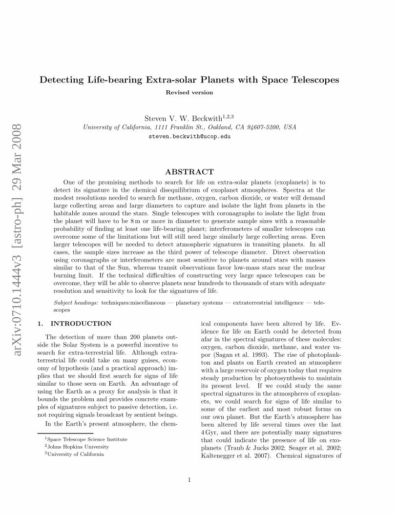
the Earth, it varies between ∼ 0.7 near 0.3µmto less than 0.3 longward of about 0.6µm anddepends on variable factors such as cloud coverand exposed land mass (Kasting et al. 1993;Turnbull et al. 2006; McCullough 2006). Weadopt a(ν) = a = 0.5 for the rest of this paperto produce a bright planet that should be mosteasily observed. As shown below, uncertainties ina(ν) will not affect the estimates in this paper sig-nificantly. The actual spectra would also includeradiative transfer effects in the atmosphere andshow absorption lines from molecules (see Fig. 1).

0.5 1 2 5 10 20

Wavelength HΜmL

10-10

10-9

10-8

10-7

10-6

FluxDensityHJyL

Spectrum of Earth from 10 pc

CO2O3

O2

H2O

H2O

H2OCO2

CO2

H2O

CH4N2O

Fig. 1.— The lower line is a synthetic spectrum ofEarth viewed from 10pc to illustrate the spectralfeatures in the Earth’s present-day atmosphere.The upper line is a combination of the solar ir-radiance and a Planck function at 286K.

Combining (1) and (3) with the assumptionsabove, the flux density of the planet is:

Fp(ν) ≈πr2

p

D2

(

1

3

r2∗

Rp2B(ν, T∗) + B(ν, Tp)

)

. (4)

This relation neglects some interesting details,such as the variable atmospheric transmission andradiative transfer effects as well as adopting as-sumptions about the albedo and phase functionthat are at best educated guesses. It turns outthat these simplifications do not affect the overallenergy balance enough to change the conclusionsof this article, but they are, nevertheless, crucialfor understanding the chemical composition of theplanet’s atmosphere.

At 10 pc, the apparent magnitude of the Earthat visual and near infrared wavelengths from (4)is about 29(AB), ∼ 10 nJy, too faint for spectrawith any existing telescopes.

3

The principal sources of noise in detecting exo-planets will be local zodiacal light, any equivalentexo-zodiacal light in the other planetary system,any residual light from the star not cancelled bythe instrument, and the planet itself. Since weare interested in the limits of nature, we assumethat starlight is completely eliminated by the tele-scope and instrument and consider only the othercontributions.

The zodiacal light has the same spectrum asthe Sun at wavelengths shorter than about 3 µm,but reduced by the optical depth of the zodia-cal cloud in the direction of observation, and itis approximately a blackbody function at thermalinfrared wavelengths with a temperature that de-pends somewhat on the viewing angle with respectto the Sun. The important point is that both thezodiacal light and exo-zodiacal light light will beuniform surface brightnesses to a good approxi-mation whose observable fluxes depend only onthe area–solid angle product (etendue) of the tele-scope and not the distance to the source. Thespectrum of the zodiacal light combines a visualoptical depth, τz ∼ 10−7, and thermal emissivity,ǫz(ν) ∼ 0.5, both strong functions of ecliptic lineof sight, to obtain the brightness of the zodiacallight as:

Iz(ν) ≈ τz[B(ν, T⊙) + ǫzB(ν, Tzody)]. (5)

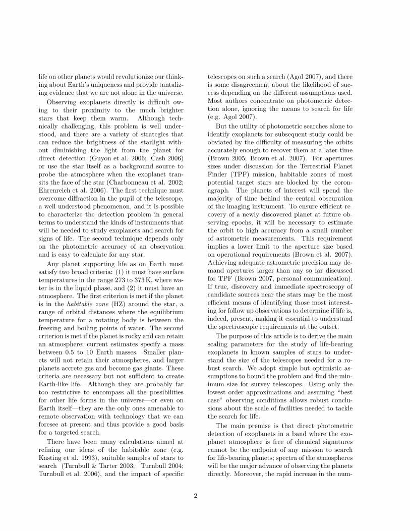
It is straightforward to calculate the exact zodiacalemission in any direction from models in the liter-ature (e.g. Leinert et al. 1998), and as a practicalmatter we will adopt a viewing angle at solar elon-gation 90 and ecliptic latitude 45 as “typical” ofa large survey seeking to minimize zodiacal back-ground: Izody(ν) is about 0.3MJy sr−1 at 0.5µmand 10MJy sr−1 at 10µm. Figure 2 compares thephoton rates seen by 4 and 8m telescopes froman Earth 10 pc away with the zodiacal light for anassumed resolving power of 100.

It is impossible to know how strong the contri-bution from the exo-zodiacal light is. It is easyto find stars with very large quantities of inter-planetary dust (Beichman et al. 2006) and starswithout detectable dust emission, so this term isone of the larger uncertainties in our estimatesas stressed by Agol (2007). The best case is ifthere is no exo-zodiacal light at all. Alternatively,if the other planetary system is identical to theSolar System, the amount of exo-zodiacal light is

just twice the local value. The easy way to un-derstand this factor of 2 is to realize that we viewthe exo-zodiacal cloud through its entire thickness,whereas we reside at the mid-plane of the local zo-diacal light (within 3) and thus look out throughonly half the optical depth in any direction. Theexo-zodiacal cloud will also be well resolved by anytelescope that can block the starlight and still ob-serve the planet. For the moment, we assume thecontribution of the exo-zodiacal light is negligible.

0.5 0.7 1 2 3 4 5 7 10 20 30

Wavelength Μm

0.01

0.1

1

10

Photonssecond

Photon rate for Earth at 10. pc

ΝΝ 0.01, 100% efficiency

8m tel.

4m tel.

Fig. 2.— The photon rates of an exo-Earth viewedfrom 10pc distance with 4m and 8 m telescopes,together with the photon rates for the local zodi-acal light for a diffraction-limited telescope.

The noise of an observation will be dominatedby the (Poisson) statistics of the incoherent pho-ton stream from the planet and the zodiacal back-ground. Denoting photon rates as Nγ(p) and

Nγ(z), respectively, the signal to noise ratio, SN ,after observing time, t, is:

SN =ηNγ(p)t

(

ηNγ(p)t + ηNγ(z)t)1/2

, (6)

=

√

ηt1

h

∆ν

ν

AtelFp(ν)√

Atel (Fp(ν) + ΩtelIz(ν)),

(7)

with the area and solid angle of the telescopedenoted Atel and Ωtel, and the overall detec-

4

tion efficiency η. For a circular telescope that isdiffraction-limited, the etendue, AtelΩtel, is justequal to the square of the observing wavelength,λ2. In the limit where the planet is far away fromthe observer (us), the photon noise is dominatedby the zodiacal light regardless of whether it islocal or around the exo-planet, since its contribu-tion is independent of both source distance andtelescope diameter, but the photon flux from theexo-planet is proportional to D−2. Equation (7)may then be written as:

SN = t1/2

√

1

h

∆ν

νη

π4d2telFp(ν)

√

(

cν

)2Iz(ν)

, (8)

∝ t1/2η1/2

(

dtel

D

)2

. (9)

The expression in (9) shows the explicit depen-dence of SN and observation time on telescopediameter and source distance in the faint limit. Ifexo-zodiacal light is comparable in brightness tothe local value, SN diminished by a factor of or-der

√3. It is useful to note that even though the

amount of exo-zodiacal light is uncertain, it intro-duces only a modest uncertainty into the signal-to-noise calculation considering many of the other un-certainties inherent in the planet detection prob-lem. However, we will assume it is zero in sub-sequent calculations to consider the best case sce-narios for taking spectra of planets.

Recasting (8) in terms of observation time forEarth at a distance is especially useful for theplanet detection problem. Using (4) and (5), Fp

and Iz can be written in terms of assumptionsabout the star, planet, and observing system pa-rameters. To simplify later calculations, we defineSN10 ≡ SN/10, Γ100 ≡ ν/∆ν/100, d8 ≡ dtel/8 m,D10 ≡ D/10 pc, and t24 ≡ t/24 hr:

t24 ≈ SN210η

−1 Γ100

(

D10

4d8

)4

(10)

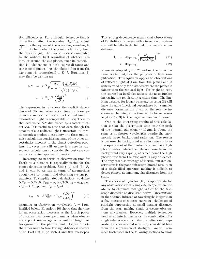
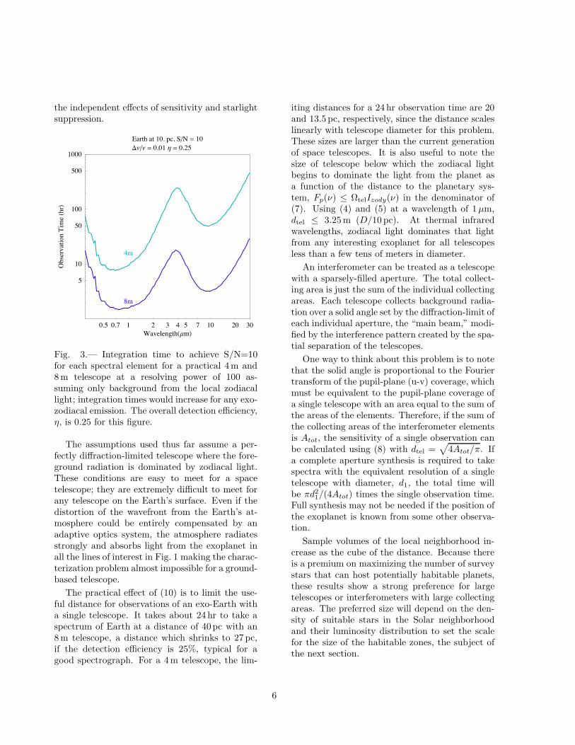
assuming an observation wavelength λ = 1 µm,justified below. Equation (10) shows that the timefor an observation increases as the fourth powerof distance over telescope diameter when observ-ing a point source against a uniform brightnessbackground in the photon limit. Figure 3 plotsthe times need to take low signal-to-noise spectraof an Earth at 10 pc with 4 and 8 m telescopes.

This strong dependence means that observationsof Earth-like exoplanets with a telescope of a givensize will be effectively limited to some maximumdistance:

Ds = 40 pc d8

(

ηt24Γ100SN2

10

)1/4

(11)

≈ 30 pc d8 (12)

where we adopted η = 0.25 and set the other pa-rameters to unity for the purposes of later sim-plification. This equation applies to observationsof reflected light at 1 µm from the planet and isstrictly valid only for distances where the planet isfainter than the zodiacal light. For bright objects,the source flux itself also adds to the noise furtherincreasing the required integration time. The lim-iting distance for longer wavelengths using (8) willhave the same functional dependence but a smallerdistance normalization given by the relative in-crease in the integration time at the longer wave-length (Fig. 3) to the negative one-fourth power.

One of the interesting results of this calcula-tion is that the observation time near the peakof the thermal radiation, ∼ 10 µm, is about thesame as at shorter wavelengths despite the enor-mously larger background radiation. The reasonis because the background noise increases only asthe square root of the photon rate, and very highphoton rates reduce the relative noise from thebackground very rapidly, at which point the highphoton rate from the exoplanet is easy to detect.The only real disadvantage of thermal infrared ob-servations is the poor diffraction-limited resolutionof a single filled aperture, making it difficult todetect planets at small angular distances from thestars.

The choice of 1µm for (10) is appropriate forany observations with a single-telescope, where theability to eliminate starlight is tied to the tele-scope diameter as discussed below. Observationsin the thermal infrared at wavelengths longer thana few microns encounter enormous challenges ofstarlight suppression at small angular distancesfrom the star, making single telescope observa-tions unworkable. However, multiple telescopesused as an interferometer or the combination of asingle telescope with a distant occulter would sep-arate the observational sensitivity considered herefrom the suppression of starlight. We will con-sider both cases in the following sections to show

5

the independent effects of sensitivity and starlightsuppression.

0.5 0.7 1 2 3 4 5 7 10 20 30

WavelengthHΜmL

5

10

50

100

500

1000

ObservationTimeHhrL

Earth at 10. pc, SN = 10

DΝΝ = 0.01 Η = 0.25

8m

4m

Fig. 3.— Integration time to achieve S/N=10for each spectral element for a practical 4m and8m telescope at a resolving power of 100 as-suming only background from the local zodiacallight; integration times would increase for any exo-zodiacal emission. The overall detection efficiency,η, is 0.25 for this figure.

The assumptions used thus far assume a per-fectly diffraction-limited telescope where the fore-ground radiation is dominated by zodiacal light.These conditions are easy to meet for a spacetelescope; they are extremely difficult to meet forany telescope on the Earth’s surface. Even if thedistortion of the wavefront from the Earth’s at-mosphere could be entirely compensated by anadaptive optics system, the atmosphere radiatesstrongly and absorbs light from the exoplanet inall the lines of interest in Fig. 1 making the charac-terization problem almost impossible for a ground-based telescope.

The practical effect of (10) is to limit the use-ful distance for observations of an exo-Earth witha single telescope. It takes about 24 hr to take aspectrum of Earth at a distance of 40pc with an8m telescope, a distance which shrinks to 27 pc,if the detection efficiency is 25%, typical for agood spectrograph. For a 4m telescope, the lim-

iting distances for a 24 hr observation time are 20and 13.5 pc, respectively, since the distance scaleslinearly with telescope diameter for this problem.These sizes are larger than the current generationof space telescopes. It is also useful to note thesize of telescope below which the zodiacal lightbegins to dominate the light from the planet asa function of the distance to the planetary sys-tem, Fp(ν) ≤ ΩtelIzody(ν) in the denominator of(7). Using (4) and (5) at a wavelength of 1 µm,dtel ≤ 3.25 m (D/10 pc). At thermal infraredwavelengths, zodiacal light dominates that lightfrom any interesting exoplanet for all telescopesless than a few tens of meters in diameter.

An interferometer can be treated as a telescopewith a sparsely-filled aperture. The total collect-ing area is just the sum of the individual collectingareas. Each telescope collects background radia-tion over a solid angle set by the diffraction-limit ofeach individual aperture, the “main beam,” modi-fied by the interference pattern created by the spa-tial separation of the telescopes.

One way to think about this problem is to notethat the solid angle is proportional to the Fouriertransform of the pupil-plane (u-v) coverage, whichmust be equivalent to the pupil-plane coverage ofa single telescope with an area equal to the sum ofthe areas of the elements. Therefore, if the sum ofthe collecting areas of the interferometer elementsis Atot, the sensitivity of a single observation canbe calculated using (8) with dtel =

√

4Atot/π. Ifa complete aperture synthesis is required to takespectra with the equivalent resolution of a singletelescope with diameter, d1, the total time willbe πd2

1/(4Atot) times the single observation time.Full synthesis may not be needed if the position ofthe exoplanet is known from some other observa-tion.

Sample volumes of the local neighborhood in-crease as the cube of the distance. Because thereis a premium on maximizing the number of surveystars that can host potentially habitable planets,these results show a strong preference for largetelescopes or interferometers with large collectingareas. The preferred size will depend on the den-sity of suitable stars in the Solar neighborhoodand their luminosity distribution to set the scalefor the size of the habitable zones, the subject ofthe next section.

6

3. Sample Sizes for Direct Observations

The interesting candidate stars will be thosewhose habitable zones can be studied after thelight from the star is suppressed to a level be-low the background. Because the starlight mustbe essentially eliminated—the Sun is ∼ 1010 timesbrighter than its reflected light from the Earth—starlight cancellation is incredibly demanding. Itis generally a far higher technical hurdle than de-tection for exo-planet observations, and it is thereason that articles on this subject often underes-timate the importance of background-limited sen-sitivity when considering exo-planet studies.

For a single telescope, starlight suppression re-quires a coronagraph that rejects light over a smallarea in the focal plane, while allowing observationof the light from outside this area. The smallestarea that can be darkened depends on the lim-iting resolution of the telescope which can neverbe smaller than the diffraction limit of the pupil.An external occulter suppresses starlight by usinga distant screen decoupled from the telescope tocreate a shadow of the starlight outside of whichexoplanets may be studied. An interferometer isessentially a sparse aperture telescope that can bephased to null starlight like a coronagraph over anangular area the depends (inversely) on the sepa-ration of the elements.

The inner working angle, θIWA, is definedas the smallest angular separation between abright star and a much fainter planet at whichthe planet can be studied with good cancel-lation of the starlight. For a single telescopewith a circular pupil, the diffraction patternis an Airy function (Born & Wolf 1999), andθIWA cannot be less than the distance to thefirst null at 1.2λ/dtel. Most realistic corona-graphs achieve inner working angles more thantwice this angle, even with nearly optimal de-signs (Guyon et al. 2006). The angle of the firstnull is typically many tens of milli-seconds of arc:1.2λ/dtel = 0.21 arcsec (λ/1 µm) (dtel/1 m)−1.

For a telescope-occulter combination or an in-terferometer, the inner working angle is not con-strained by the diameter of the light collectingtelescope(s). An occulter produces a fixed innerworking angle determined by its size and distancefrom the telescope. The inner working angle of aninterferometer depends on the maximum distance

between individual elements (telescopes) and willvary with position angle on the sky, depending itsconfiguration. The resolution of an interferome-ter varies with wavelength in the same manner asa coronagraph, allowing us to characterize the in-ner working angle as a fraction of the diffraction-limit of the effective diameter of the telescope,θIWA = fθ1.2λ/dtel for any system, with fθ ≥ 1for a coronagraph, fθ ≪ 1 for an interferometer,and fθ(λ) a function of wavelength for an occulterbut generally less than one for the wavelengths ofobservation.

In all cases, the size of the star sample availablefor study will increase as the inner working an-gle decreases, making the smaller habitable zonesaround numerous low-luminosity stars observableat any distance. Put differently, as θIWA shrinks,the minimum mass of main sequence stars avail-able for study decreases, and the sample size growsfrom the inclusion of low mass stars.

We can simplify this problem by deriving scal-ing relationships for the size of the habitable zonesaround stars as a function of stellar parametersand characterizing the samples in terms of thepresent day mass function of stars that gives theirnumber density as a function of stellar mass. Therelative advantages of the different star suppres-sion techniques will then emerge as a comparisonof sample sizes for specific observing techniques.

Almost all the interesting spectral features inthe Earth’s atmosphere are longward of 0.7µm(Fig. 1.) A spectrum should extend to at least1 µm to be analyzed for evidence of disequilib-rium chemistry indicative of life, and longer wave-lengths bring in even more interesting features.We adopt λ = 1 µm as the minimum workingwavelength to look for signs of life in spectra andnote the desirability of observations to look for sig-natures of ozone, methane, and water that havestrong bands throughout the thermal infrared be-yond 10µm, where integration times are near asecond minimum as seen in Fig. 3.

The size of the habitable zone depends on thestellar luminosity. The total thermal emission,4πr2

pσT 4p , must equal the total amount of absorbed

starlight, (1−a)L∗/(4πR2p). The planet’s temper-

ature, Tp, is bounded between the freezing andboiling points of water, 273 K ≤ Tp ≤ 373 K, anecessary but not sufficient condition for life as itis on Earth. We assume for this calculation that all

7

the starlight is absorbed (a = 0) to maximize thehabitable zone radii. This condition is sufficient tocompute the inner and outer habitable zone radiifor a star of luminosity, L∗ using general formulaefor the orbital radius, Rp, of a rotating planet atequilibrium temperature, Tp:

Rp =

√

L∗

16πσT 4p

, (13)

=1

2

(

T∗

Tp

)2

r∗. (14)

The inner and outer radii of the habitable zoneare obtained from (14) with Tp = 373 and273K, respectively. Effects such as greenhousewarming or low absorption of starlight via highalbedo will change these radii by modest factors(Kasting et al. 1993) in opposite directions; forexample, the effective temperature of the Earthis ∼ 255K (Orton 2000) and the albedo is ∼ 0.5but the greenhouse effect keeps the surface warm.These corrections are not large enough to changethe overall conclusions of this paper, however, andwe will subsequently ignore them in the interestof simplicity.

Using (13) to compute the radii boundingthe habitable zone, θIWA determines the maxi-mum angular area that can be blocked to achievestarlight suppression for a star at a known dis-tance and luminosity. By examining large sam-ples of stars, it is possible to determine how manyhave habitable zones that can be observed witha telescope or telescope system (interferometer ortelescope and occulter).

To the accuracy required for the treatmentin this paper, we express the stellar parametersin terms of the normalized stellar mass, m ≡m∗/M⊙, as follows:

L∗ ≈ L⊙ m4 (15)

r∗ ≈ r⊙ m (16)

T∗ ≈ T⊙ m0.5 (17)

The approximations are good to about 25% for thelocal sample; for the Zero Age Main Sequence, thecoefficients in front of the three equations wouldbe 1.2L⊙, 0.96r⊙, and 1.1T⊙, respectively, and theexponents would be 3.8, 0.92, and 0.49, respec-tively.

These relationships allow us to recast the equa-tions for observing the atmospheres of exoplanetsin terms of stellar mass. In particular, we can sep-arate the impact on sample size of the collectingarea from inner working angle, allowing any ob-serving system to be optimized when trading offthese two parameters.

The star is relevant only to the size of the hab-itable zone through (14), the planet always havingapproximately the same spectrum (we will adoptT⊕ = 285K to correspond to earlier sections):

Rp =1

2

(

T⊙

Tp

)2

m2 r⊙ (18)

= 1.0 AU

(

Tp

T⊕

)−2

m2 (19)

The size of the habitable zone is proportional to√L∗ ∝ m2 from (13) and (15). For any inner

working angle, there is a minimum mass star forwhich the habitable zone might be observed at anydistance, Rp(mmin) = θIWAD. We will specify theinner working angle as a multiple of the diffractionlimit of a circular pupil, θIWA = fθ(1.2λµ/dtel)and for generality define the equivalent diameterof the telescope system in terms of the collectingarea, dtel =

√

4Atel/π. Then, the maximum dis-tance to a star of normalized mass, m, where thehabitable zone can still be resolved is:

DIWA(m) = Rp/θIWA (20)

≈ 30 pc d8f−1θ

(

Tp

T⊕

)−2

m2 (21)

For any star, the maximum distance for spectro-scopic observations will be the lesser of DIWA orDs, the limit from the integration time in (12).The minimum stellar mass whose habitable zoneis observable at distance, D, is:

mmin =

(

fθ

d8

D

30 pc

)1/2Tp

T⊕

(22)

The present day mass function, ξ(m), of localstars above the nuclear burning limit is well ap-proximated by two power laws1 in stellar mass(Reid et al. 2002):

ξ(m) = 0.02 pc−3 m−αm (23)

1Other choices are possible (Kroupa 2001), but this choicefits both the 8 pc sample and the more extended sample ofsolar mass stars to 25 pc.

8

with α(0.08 ≤ m < 1.0) = 1.1 ≈ 1 and α(m ≥ 1.0)= 5.2 ≈ 5. The PDMF is defined such that thenumber density of stars in the mass range m tom + dm is ξ(m)dm. The large exponent for theupper end of the mass range describes the actualnumber density of stars above a few solar massesas opposed to the initial mass function which isderived by correcting for stellar evolution.

The sample size distribution for direct observa-tions follows from (23) using the maximum volumefor each stellar mass:

dNd/dm =4π

3D3ξ(m) (24)

where D is either DIWA or Ds. The stellar massfor which Ds becomes the limiting distance de-pends on the rejection factor, fθ, and the placein the habitable zone where the planet resides,governed by Tp. If we assume a perfect corona-graph observing Earth, then fθ(Tp/T⊕) ≈ 1, andDs < DIWA for m > 1, exactly where the expo-nent in ξ(m) changes value. The total sample forall masses above 0.1M⊙ is:

Nd =4π

3

(

∫ 1

0.1

D3IWA(m)ξ(m)dm

+D3s

∫ ∞

1

ξ(m)dm)

(25)

≈ 1900 f−3θ

(

Tp

T⊕

)−6

d38 (26)

The sample size depends strongly on the effec-tive diameter of the telescope, inner working angle,and working wavelength in the low-mass limit. Itdepends weakly on the overall detection efficiency,integration time, signal-to-noise ratio, and spec-tral resolving power.

3.1. Samples for Coronagraphs

Direct observations of planets with corona-graphs tend to be limited by the inner workingangle and benefit from the largest possible hab-itable zone. Evaluating (26) with fθ = 2, thesample size as a function of telescope diameter is:

Nd ≈ 280

(

Tp

T⊕

)−6

d38 (27)

An 8m telescope with an excellent coronagraphshould have almost than 300 stars around which

direct characterizations of Earth-like planets couldbe made spectroscopically, assuming every starwhere suitable for observation (e.g. no binaries).But the dependence on the third power of tele-scope diameter shows that the best one could dowith a 4m telescope is about 35 stars, and thisis the total sample without correction for multiplestar systems and stars that might not be suitablefor life. On the other hand, a very large telescope,16m, say, could study thousands of stars to char-acterize terrestrial planets.

3.2. Samples for Compound Telescopes

The samples can grow rapidly when fθ is lessthan 1. Use of an external occulter should producefθ ∼ 1, and an interferometer could give fθ ≪ 1,although the instantaneous coverage of the (u, v)plane is sparse and would be of limited value unlessthe precise location of the planet were well knownat the time of the observation.

Evaluating (25) for the case fθ = 0.1 and Tp =T⊕ yields:

Nd ≈ 3300 d38, for fθ = 0.1 (28)

This is the sample a good interferometer mightaccess. An occulter can reduce fθ to less than 1(e.g. Cash 2006), but the sample size grows ratherslowly with decreasing fθ owing to the sensitivitylimit. The typical size of an occulter to producefθ ≤ 1 coupled with its distance from the telescopeto produce a small inner working angle will makea practical occulter difficult to use.

These examples show that the gain from us-ing a larger telescope comes about mainly fromthe rapid increase in sensitivity with aperture size,d−2tel , and the rapid increase in sample size owing

to the larger volume probed: N ∼ D3 ∼ d3tel.

The use of an external occulter helps mitigatethe technical demands of creating a nearly per-fect coronagraph, although it will drive some verystrong technical demands of its own—alignmentof a ∼ 60m structure at 400,000km from a spacetelescope and moving it around to sample differentstars will be no mean feat. Large telescopes willstill have an enormous advantage for searching forsigns of life on exoplanets.

9

4. Spectra of Transiting Exoplanets

It is possible to distinguish very slight differ-ences in the light curve at different wavelengthsas an exoplanet transits the face of its centralstar. These differences result from transmissionspectrum of the star through the planet’s atmo-sphere making the apparent size of the planetlarger at wavelengths where the atmosphere isopaque. Charbonneau et al. (2002) and Vidal-Madjur et al. (2003, 2004) demonstrated the util-ity of this method by detecting sodium, hydrogen,oxygen, and carbon in the extended atmosphere ofthe transiting exoplanet, HD 209458b, using theSTIS spectrograph on 2.4m Hubble Space Tele-scope. Tinetti et al. (2007) used the SpitzerSpace Telescope in a similar way to detect H2Oin HD 189733b. Transits provide an alternativeway to look for the signatures of life in exoplanets(Seager & Sasselov 2000).

As a planet passes across the face of a star,the starlight dims by approximately the ratio ofthe area of the planet to that of the star, ∆p ≈πr2

p/πr2∗, where we ignore the modest effect of limb

darkening. If the scale height of the atmosphere ishatm and an atmospheric absorption feature hasthe effect of blocking all light to x scale heightsabove the surface, there will be a small differencein the depth of the light curve viewed at the wave-length of the feature:

∆atm − ∆p =(rp + xhatm)2 − r2

p

r2∗

, (29)

≈ 2xhatmrp

r2∗

, (30)

where the approximation assumes xhatm ≪ rp.For the Earth crossing the face of the Sunseen from afar, this an excellent approximation:hatm ≈ 9 km, rp ≈ 6400km, and ∆atm − ∆p =2 × 10−7 for x = 1. The scale height of the atmo-sphere depends on the density and temperatureof the planet through the usual thermodynamicrelation:

hatm =kTp

µg, (31)

=3kTp

4πGµρrp, (32)

where g is the gravitational acceleration at theplanet’s surface, µ is the mean molecular mass,

and ρ is the mean density of the planet2. Recast-ing (30) in terms of the density:

∆atm − ∆p ≈ x3kTp

2πGµρr2∗

. (33)

This result shows somewhat non-intuitively thatthe atmospheric signature for a planet in the hab-itable zone is independent of the planet’s size; tofirst order, it depends only on the density and tem-perature, the latter of which lies between the freez-ing and boiling points of water, thus bounding therange of possibilities. The stronger gravitationalfield of larger planets decreases the scale height tocompensate for the increase in the planet’s radius.

The number of scale heights for the effectivecross section, x, depends on the strength of theabsorption lines. In the Earth’s atmosphere, thestrength of the absorption lines is normally ex-pressed in terms of the vertical optical depth fromthe ground to space. For a molecule whose numberdensity, ni, as a function of height, z, is exponen-tial with scale height, hatm, and absorption crosssection per molecule, σi, the vertical optical depthis τ0 =

∫∞

0niσi exp(−z/hatm) dz = niσihatm.

Then the optical depth through the atmospherealong a line with an impact parameter x scaleheights above the surface is given by:

τ(x) = τ0

∫ ∞

−∞

e−

„

q

(x+r′

p)2+y2−r′

p

«

dy (34)

= 2τ0er′

p

(

r′p + x)

K1(r′

p + x), (35)

≈ τ0

√2π(

r′p + x)

1

2 e−x (36)

where r′p = rp/hatm, K1 is a modified Bessel func-tion, and the approximation assumes r′p + x ≫ 1.The value of x that gives the effective atmosphericcross section for any absorption line seen in tran-sit is the solution to (36) that gives τ(x) = 1. Forr′p ≫ x, the solution is:

x ≈ 0.92 +1

2ln

(

rp

hatm

)

+ ln(τ0) (37)

≈ 4.20 + ln(τ0) for r′p =6400

9. (38)

2The density of a planet increases slightly with mass as theinterior equation of state changes (Seager et al. 2007), butthe effect is small enough to be ignored at this level ofapproximation.

10

The lines shortward of 1µm in Fig. 1 havevertical optical depths, τ0, between 0.1 and 1(Crisp 2000), meaning x is between 2 and 4. Thereare very strong H2O lines at wavelengths of a fewmicrons, in principle giving x ∼ 10, although forthe Earth itself, water vapor is confined to thetropopause within a single scale height, so the lackof vertical mixing means that x(H2O) ∼ 1 despitethe large τ0. The important result of (37) is thatthe effective cross section within an absorption linedepends on the logarithm of the line optical depth;even order of magnitude uncertainties in the totalatmospheric density affect the transit depths mod-estly.

Detecting the absorption lines in a transit ob-servation means achieving very high photometricaccuracy in the difference spectrum in and out ofthe line. The best photometric accuracy that canbe achieved during a transit is if all the starlight isdetected with perfect efficiency and the only noisesource is the statistical fluctuation of the photonrate as assumed in (7). Using the formalism abovefor measurement time, tobs, and assuming the dif-ference of two measurements:

σNγ

Nγ=

(

2

Nγtobs

)1/2

, (39)

=

(

π

8h

∆ν

νF∗(ν)d2

teltobs

)−1/2

. (40)

The total observation time will be the time of asingle transit times the number of transits. Viewedfrom a great distance, the maximum transit timeis just ttrans = 2r∗/vp = 2r∗

√

Rp/GM∗, and thetime for an average transit (i.e. not across theequator) is just one half this value. The numberof transits observed during the lifetime of a spacemission, tm, is just nP = tm/P , with nP truncatedto an integer . The total observation time is:

tobs = nP ttrans (41)

= tm1

2π

√

GM∗

R3p

2r∗

√

Rp

GM∗

(42)

= tm1

π

r∗Rp

(43)

= tm2

π

(

Tp

T∗

)2

(44)

We used (14) to express Rp in terms of the temper-atures to yield another non-intuitive result: the to-

tal observation time decreases as the stellar effec-tive temperature increases. This effect combinedwith the lower contrast for a transit is more thanenough to offset the advantage of having a brighterstar with a higher photon rate:

SNtr =∆atm − ∆p

σNγ/Nγ

(45)

= x3kT 2

p dtel

4πGµρr2∗T∗

(

1

h

∆ν

νF∗(ν)tm

)1/2

(46)

= x3kT 2

p dtel

4πGµρr2∗T∗

(

1

hΓtm

)1/2

×(

πr2∗

D2

2hν3

c2

1

exp( hνkT∗

) − 1

)1/2

(47)

where we approximated the flux density from thestar as a blackbody in (47).

Using the same approach as in §3 to expressthe stellar quantities, T∗ and r∗, in terms of thestellar mass, setting x = 4 from (38), adoptingµ = 30 amu and ρ = 5g cm−3, the signal-to-noiseratio for a transit observation is:

SNtr = 240d8

Dpc

(

Tp

T⊕

)2

m−1.5

×(

exp(2.5m−0.5) − 1)−1/2

(48)

The signal-to-noise ratio for transit observa-tions of terrestrial planets in the habitable zonesaround stars increases rapidly with decreasingstellar mass: small stars are strongly favored overmassive stars at all distances, both because thetransit depths are larger and the observation timesare longer, more than offsetting the increasedphoton rate with increasing stellar temperature.This is a general result that also applies to thephotometric detection planetary transits, not justthe highly challenging observation of atmosphericlines. Notice also that the signal-to-noise ratio de-pends linearly on d8/D, a slower rate than forbackground limited photometric observations of(7).

The challenge of using transits to detect atmo-spheric features is illustrated by evaluating (40)for the Earth/Sun system at a distance of 10 pc.A single transit of the Earth across the diame-ter of the Sun takes 16 hours during which an8m telescope would capture 3 × 1013 photons at

11

a spectral resolution of 1/Γ = ∆ν/ν = 0.01 at1µm. The fractional uncertainty in the differ-ence in light curves at two frequencies would beσNγ

/Nγ = 2.6 × 10−7, yielding a signal-to-noiseratio of 3 on for a feature with τ(hatm) = 1and x = 4, such as the oxygen lines. Since thissignal-to-noise ratio is too small for most featuresof interest and the required telescope is large, itwill probably be impossible to detect signatures ofmore distant Earths using transits at these wave-lengths. However, large telescopes might be ableto detect deep water features with τ(hatm) ∼ 104

at wavelengths of a few microns with sufficient col-lecting area, if the water vapor extends throughoutthe atmosphere, unlike the situation on Earth.

The greater complication with this technique,however, is that the orbital plane of the planetmust be aligned with the line of sight for a transitto be observed. The a priori probability of align-ment, assuming orientations uniformly distributedwithin the celestial sphere and requiring only thatthe planet graze some part of the stellar surface,is:

f =r∗Rp

, (49)

= 2

(

Tp

T∗

)2

, (50)

where we have used (14) to derive (50). The frac-tion, f , is much less than unity even for cool stars,meaning we would need many candidate stars toensure that even a few transiting planets would beobserved.

4.1. Samples for transit observations

The maximum distance for transit observationsof a star is derived from (48) by solving for Dt.Then, using (23) for the PDMF, the sample sizedistribution, dNt/dm, is just (4π/3)D3

t (m)ξ(m):

dNt/dm = 1000 d38

(

Tp

T⊕

)6

× m−α2

(exp(2.5m−0.5) − 1)3/2

(51)

with α2 = 5.5 for m ≤ 1, or α2 = 9.5 for m >1. The transit technique strongly favors the lowermass stars and hot planets near the inner edge ofthe habitable zone. Equation (51) has a strong

maximum near m = 0.12 and falls off very steeplyabove m=1.

One other quantity of interest is the expectednumber of stars in the sample in which the orbitalplanes will align so that the planets will transitthe face of the star. Using (50) with the formalismabove, the expected number is:

dNet/dm = f(m)dNt/dm (52)

= 2 d38

(

Tp

T⊕

)8

× m−α3

(exp(2.5m−0.5) − 1)3/2

(53)

with α3 = 6.5 for m ≤ 1, or α3 = 10.5 for m >1. The number of observed transits is so heavilyweighted toward low mass stars that the techniquefavors those near the nuclear burning limit.

Integrating (51) and (53) from m = 0.1 to ∞yields the total sample size and expected numberof in the sample in which the orbital plane of theplanet is aligned for transits:

Nt ≈ 500 d38

(

Tp

T⊕

)6

(54)

Net ≈ 5 d38

(

Tp

T⊕

)8

(55)

The final two columns of Table 3 contains the to-tal number of candidates and expected number ofobserved transits from (54), and (55).

Notice that the assumptions used to arrive at(55) are for the best case of maximum transit timeand perfect detection efficiency, and there is evena slight increase in the observing time if the num-ber of transits is not truncated to an integer; thisresult is the best we can do.

Figure 4 shows how the samples for direct andtransit observations are distributed across spectraltype. These are complementary techniques, withdirect observations favoring stars of about 1M⊙,and transit observations favoring low mass starsnear the nuclear burning limit. It will be usefulto use both techniques to characterize the atmo-spheres of planets around stars of all masses.

These results again point to the great advan-tage that large telescopes bring to the study oftransiting exoplanets. An 8 m telescope shouldsee of order 5 transiting planets in the terrestrial

12

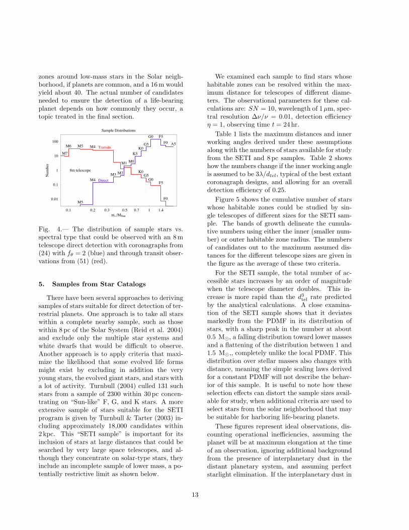
zones around low-mass stars in the Solar neigh-borhood, if planets are common, and a 16m wouldyield about 40. The actual number of candidatesneeded to ensure the detection of a life-bearingplanet depends on how commonly they occur, atopic treated in the final section.

0.1 0.2 0.3 0.5 0.7 1 1.4

mMSun

0.01

0.1

1

10

100

Number

Sample Distributions

A5F0

F5G0

G5K0

K5

M0M1

M2M3

M4

M5F0

F5G0

G5K0

M4M5M6

M7

8m telescope

Transits

Direct

Fig. 4.— The distribution of sample stars vs.spectral type that could be observed with an 8 mtelescope direct detection with coronagraphs from(24) with fθ = 2 (blue) and through transit obser-vations from (51) (red).

5. Samples from Star Catalogs

There have been several approaches to derivingsamples of stars suitable for direct detection of ter-restrial planets. One approach is to take all starswithin a complete nearby sample, such as thosewithin 8 pc of the Solar System (Reid et al. 2004)and exclude only the multiple star systems andwhite dwarfs that would be difficult to observe.Another approach is to apply criteria that maxi-mize the likelihood that some evolved life formsmight exist by excluding in addition the veryyoung stars, the evolved giant stars, and stars witha lot of activity. Turnbull (2004) culled 131 suchstars from a sample of 2300 within 30 pc concen-trating on “Sun-like” F, G, and K stars. A moreextensive sample of stars suitable for the SETIprogram is given by Turnbull & Tarter (2003) in-cluding approximately 18,000 candidates within2 kpc. This “SETI sample” is important for itsinclusion of stars at large distances that could besearched by very large space telescopes, and al-though they concentrate on solar-type stars, theyinclude an incomplete sample of lower mass, a po-tentially restrictive limit as shown below.

We examined each sample to find stars whosehabitable zones can be resolved within the max-imum distance for telescopes of different diame-ters. The observational parameters for these cal-culations are: SN = 10, wavelength of 1µm, spec-tral resolution ∆ν/ν = 0.01, detection efficiencyη = 1, observing time t = 24hr.

Table 1 lists the maximum distances and innerworking angles derived under these assumptionsalong with the numbers of stars available for studyfrom the SETI and 8 pc samples. Table 2 showshow the numbers change if the inner working angleis assumed to be 3λ/dtel, typical of the best extantcoronagraph designs, and allowing for an overalldetection efficiency of 0.25.

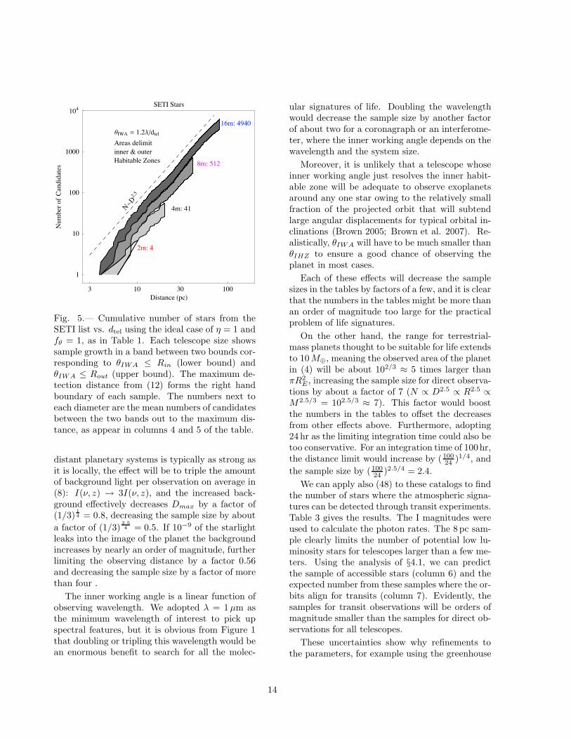
Figure 5 shows the cumulative number of starswhose habitable zones could be studied by sin-gle telescopes of different sizes for the SETI sam-ple. The bands of growth delineate the cumula-tive numbers using either the inner (smaller num-ber) or outer habitable zone radius. The numbersof candidates out to the maximum assumed dis-tances for the different telescope sizes are given inthe figure as the average of these two criteria.

For the SETI sample, the total number of ac-cessible stars increases by an order of magnitudewhen the telescope diameter doubles. This in-crease is more rapid than the d3

tel rate predictedby the analytical calculations. A close examina-tion of the SETI sample shows that it deviatesmarkedly from the PDMF in its distribution ofstars, with a sharp peak in the number at about0.5 M⊙, a falling distribution toward lower massesand a flattening of the distribution between 1 and1.5 M⊙,, completely unlike the local PDMF. Thisdistribution over stellar masses also changes withdistance, meaning the simple scaling laws derivedfor a constant PDMF will not describe the behav-ior of this sample. It is useful to note how theseselection effects can distort the sample sizes avail-able for study, when additional criteria are used toselect stars from the solar neighborhood that maybe suitable for harboring life-bearing planets.

These figures represent ideal observations, dis-counting operational inefficiencies, assuming theplanet will be at maximum elongation at the timeof an observation, ignoring additional backgroundfrom the presence of interplanetary dust in thedistant planetary system, and assuming perfectstarlight elimination. If the interplanetary dust in

13

3 10 30 100

Distance pc

1

10

100

1000

104

NumberofCandidates

SETI Stars

2m: 4

4m: 41

8m: 512

16m: 4940

Areas delimit

inner & outer

Habitable Zones

ΘIWA 1.2Λdtel

ND2.5

Fig. 5.— Cumulative number of stars from theSETI list vs. dtel using the ideal case of η = 1 andfθ = 1, as in Table 1. Each telescope size showssample growth in a band between two bounds cor-responding to θIWA ≤ Rin (lower bound) andθIWA ≤ Rout (upper bound). The maximum de-tection distance from (12) forms the right handboundary of each sample. The numbers next toeach diameter are the mean numbers of candidatesbetween the two bands out to the maximum dis-tance, as appear in columns 4 and 5 of the table.

distant planetary systems is typically as strong asit is locally, the effect will be to triple the amountof background light per observation on average in(8): I(ν, z) → 3I(ν, z), and the increased back-ground effectively decreases Dmax by a factor of(1/3)

1

4 = 0.8, decreasing the sample size by about

a factor of (1/3)2.54 = 0.5. If 10−9 of the starlight

leaks into the image of the planet the backgroundincreases by nearly an order of magnitude, furtherlimiting the observing distance by a factor 0.56and decreasing the sample size by a factor of morethan four .

The inner working angle is a linear function ofobserving wavelength. We adopted λ = 1 µm asthe minimum wavelength of interest to pick upspectral features, but it is obvious from Figure 1that doubling or tripling this wavelength would bean enormous benefit to search for all the molec-

ular signatures of life. Doubling the wavelengthwould decrease the sample size by another factorof about two for a coronagraph or an interferome-ter, where the inner working angle depends on thewavelength and the system size.

Moreover, it is unlikely that a telescope whoseinner working angle just resolves the inner habit-able zone will be adequate to observe exoplanetsaround any one star owing to the relatively smallfraction of the projected orbit that will subtendlarge angular displacements for typical orbital in-clinations (Brown 2005; Brown et al. 2007). Re-alistically, θIWA will have to be much smaller thanθIHZ to ensure a good chance of observing theplanet in most cases.

Each of these effects will decrease the samplesizes in the tables by factors of a few, and it is clearthat the numbers in the tables might be more thanan order of magnitude too large for the practicalproblem of life signatures.

On the other hand, the range for terrestrial-mass planets thought to be suitable for life extendsto 10 M⊕, meaning the observed area of the planetin (4) will be about 102/3 ≈ 5 times larger thanπR2

E , increasing the sample size for direct observa-tions by about a factor of 7 (N ∝ D2.5 ∝ R2.5 ∝M2.5/3 = 102.5/3 ≈ 7). This factor would boostthe numbers in the tables to offset the decreasesfrom other effects above. Furthermore, adopting24 hr as the limiting integration time could also betoo conservative. For an integration time of 100hr,the distance limit would increase by (100

24)1/4, and

the sample size by (10024

)2.5/4 = 2.4.

We can apply also (48) to these catalogs to findthe number of stars where the atmospheric signa-tures can be detected through transit experiments.Table 3 gives the results. The I magnitudes wereused to calculate the photon rates. The 8 pc sam-ple clearly limits the number of potential low lu-minosity stars for telescopes larger than a few me-ters. Using the analysis of §4.1, we can predictthe sample of accessible stars (column 6) and theexpected number from these samples where the or-bits align for transits (column 7). Evidently, thesamples for transit observations will be orders ofmagnitude smaller than the samples for direct ob-servations for all telescopes.

These uncertainties show why refinements tothe parameters, for example using the greenhouse

14

effect to increase the size of the habitable zoneslightly or trying to estimate the exo-zodiacal lightbackground precisely, can complicate the analy-sis without bringing any greater insight into thelikelihood of detecting life-bearing planets. More-over, the assumptions used here are optimisticabout technological advances for observing exo-planets. There are no margins built in: we assumethat all the starlight is rejected, there is no exo-zodiacal background, the detection efficiency isnearly ideal, and there is sufficient resolution whenthe inner working angle is equal to the size of thehabitable zone. The numbers of candidate starslisted in Table 2 only take into account marginsfor θIWA and detection efficiency, and we believethey may safely be taken as upper limits to thenumber of observable stars for a given telescopediameter, allowing for some margin in the uncer-tainties of the properties of exoplanets. Character-izing the atmospheres of Earth-like planets aroundother stars will be a challenging problem for theforeseeable future.

6. Likelihood of Life Bearing Planets

The number of life-bearing planets that canbe detected in a survey will depend on the frac-tion of accessible candidate stars with an Earth-like planet in the habitable zones around the staras well as likelihood that the planets develop lifequickly enough so that it starts to dominate theplanet’s atmospheric chemistry. This fraction isconventionally called ηEarth.

3

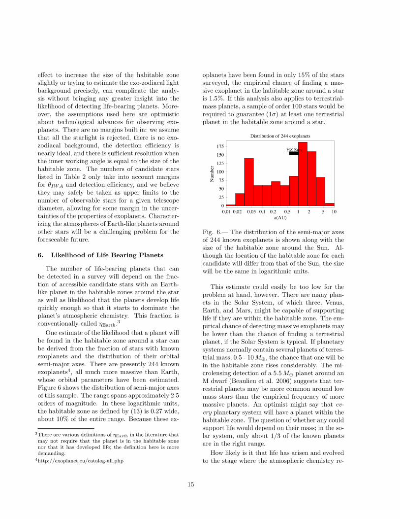
One estimate of the likelihood that a planet willbe found in the habitable zone around a star canbe derived from the fraction of stars with knownexoplanets and the distribution of their orbitalsemi-major axes. There are presently 244 knownexoplanets4, all much more massive than Earth,whose orbital parameters have been estimated.Figure 6 shows the distribution of semi-major axesof this sample. The range spans approximately 2.5orders of magnitude. In these logarithmic units,the habitable zone as defined by (13) is 0.27 wide,about 10% of the entire range. Because these ex-

3There are various definitions of ηEarth in the literature thatmay not require that the planet is in the habitable zonenor that it has developed life; the definition here is moredemanding.

4http://exoplanet.eu/catalog-all.php

oplanets have been found in only 15% of the starssurveyed, the empirical chance of finding a mas-sive exoplanet in the habitable zone around a staris 1.5%. If this analysis also applies to terrestrial-mass planets, a sample of order 100 stars would berequired to guarantee (1σ) at least one terrestrialplanet in the habitable zone around a star.

0.01 0.02 0.05 0.1 0.2 0.5 1 2 5 10

aHAUL

0

25

50

75

100

125

150

175

Number

Distribution of 244 exoplanets

HZ Sun

Fig. 6.— The distribution of the semi-major axesof 244 known exoplanets is shown along with thesize of the habitable zone around the Sun. Al-though the location of the habitable zone for eachcandidate will differ from that of the Sun, the sizewill be the same in logarithmic units.

This estimate could easily be too low for theproblem at hand, however. There are many plan-ets in the Solar System, of which three, Venus,Earth, and Mars, might be capable of supportinglife if they are within the habitable zone. The em-pirical chance of detecting massive exoplanets maybe lower than the chance of finding a terrestrialplanet, if the Solar System is typical. If planetarysystems normally contain several planets of terres-trial mass, 0.5 - 10M⊕, the chance that one will bein the habitable zone rises considerably. The mi-crolensing detection of a 5.5M⊕ planet around anM dwarf (Beaulieu et al. 2006) suggests that ter-restrial planets may be more common around lowmass stars than the empirical frequency of moremassive planets. An optimist might say that ev-

ery planetary system will have a planet within thehabitable zone. The question of whether any couldsupport life would depend on their mass; in the so-lar system, only about 1/3 of the known planetsare in the right range.

How likely is it that life has arisen and evolvedto the stage where the atmospheric chemistry re-

15

flects its presence? On Earth, life arose quicklyand began to alter the atmosphere in ways thatmight have been detectable from afar by anage of order 1Gyr (Kaltenegger et al. 2007). Ittook more than 3.5 billion years to producesubstantial amounts of oxygen via photosyn-thetic organisms to a state we would recognizetoday (Kasting & Catling 2003, and referencestherein). The oxygen would disappear from theatmosphere in few million years if life were tocease, and CO2 would dissolve in the oceanswithin a few thousand years, eliminating the mostprominent atmospheric signature of organismson Earth. It required a series of unlikely acci-dents for Earth to alter its atmosphere, suggest-ing that it may not occur easily on other planets(Ward & Brownlee 2000).

Thus, an estimate made a priori of the fractionof stars with life-bearing planets depends entirelyon how much faith we have that all the circum-stances are favorable, that is the number of ap-parent miracles we are willing to believe. If allstars have planetary systems (but only 15% havemassive planets), and all planetary systems haveat least one Earth-like planet within the habitablezone, and this planet always evolves life to domi-nate its atmospheric chemistry, then nearly 100%of the suitable stars will have planets indicative oflife, i.e. ηEarth ∼ 1. Even a 4m space telescopemight be adequate to carry out the first observa-tions.

On the other hand, if only 15% of stars typicallyhave planetary systems of which the likelihood ofan Earth-like planet in the terrestrial zone is only30% and the chance of evolving life is less than1, then ηEarth < 0.05, and it may be much lessthan this value if the sequence of events leadingto life-signatures in the atmospheric spectra aremore rare than common; many of the low massstars making up the majority of the complete 8 pcsample are likely to be too young to have evolvedlife as on Earth (Reid et al. 2007). A pessimistmight conclude that ηEarth << 0.01.

We believe that a pragmatic approach to thestudy of life-bearing exoplanets will require morethan 100 candidate stars to yield at least onewith the characteristics we seek, requiring a large(> 8 m) space telescope. A very large space tele-scope of order 16m diameter would have thou-sands of candidate stars to study and, while tech-

nically challenging to build, would also be an ex-cellent tool for examining exoplanets found byother means, such as spectra-photometry of thetransits discussed in §4.

The range of uncertainty will narrow consider-ably when the results of the Kepler mission to findEarth-like planets around distant stars are knownin a few years. However, Kepler is observing morethan 105 distant (> 1 kpc) stars, very few of whichwill be close enough to look for atmospheric sig-natures. In the absence of very large space tele-scopes to find and study nearby stars, it will stillleave open the question about about the likelihoodof life outside of the Solar system.

I am grateful to an anonymous referee who sug-gested several qualitative changes in the approachto this paper, vastly improving it. I also thankRobert Brown, Peter McCullough, James Pringle,Marc Postman, Neill Reid, Kailash Sahu, DavidSoderblom, and Jeff Valenti for their advice andto Mike Hauser and Matt Mountain for encourage-ment to pursue this work. This research was sup-ported by NASA through its contract to AURAand the Space Telescope Science Institute and theUniversity of California.

16

REFERENCES

Agol, E. 2007, MNRAS, 374, 1271.

Beaulieu, J.-P. et al. 2006, astro-ph/0601563.

Beichman, C. A. et al. 2006, ApJ, 639, 1166.

Born M. and Wolf E. (1999). Principles of optics.

Seventh edition, Cambridge University Press,Cambridge, UK.

Brown, R. A. 2005, ApJ, 624, 1010.

Brown, R. A., Shaklan, S. B., and Hunyadi, S.L. 2007, Coronagraph Workshop 2006, JPLPublication 02-02 7/07, W. A. Traub ed.Pasadena:JPL, p. 53.

Cash, W. 2006, Nature, 442, 51.

Charbonneau, D., Brown, t. M., Noyes, R. W.,and Gilliland, R. L. 2002, ApJ, 568, 377.

Crisp, D. 2000, in Allen’s Astrophysical Quan-

tities, Fourth edition, (AIP Press, Springer-Verlag, New York), p. 268.

Ehrenreich, D., Tinetti, G., Lecavelier des Etangs,A., Vidal-Madjar, A., and Selsis, F. 2006, A&A,448, 379.

Guyon, O., Pluzhnik, E. A., Kuchner, M. J.,Collins, B., and Ridgway, S. T. 2006, ApJS,167, 81.

Kaltenegger, L., Traub, W.A., Jucks, K.W. 2007,ApJ, 658, 598.

Kasting, J. F. and Catling, D. 2003, ARA&A, 41,429.

Kasting, J., Whitmire, D., and Reynolds, R. 1993,Icarus, 101, 108.

Kroupa, P. 2001, MNRAS, 322, 231.

McCullough, P. R. 2006, astro-ph/0610518.AJ,124, 2721.

Orton, G. S. 2000, in Allen’s Astrophysical Quan-

tities, Fourth edition, (AIP Press, Springer-Verlag, New York), p. 300.

Reid, I. N., Cruz, K. L, Allen, P., Mungall, F.,Kilkenny, D., Liebert, J., Hawley, S. L., Fraser,O. J., Covery, K. R., Lowrance, P., Kirkpatrick,J. D., and Burgasser, A. J. 2004, AJ, 128, 463.

Reid, I. N., Hawley, S. L., and Gizis, J. E. 2002,AJ, 124, 2721.

Reid, I. N., Turner, E. L., Turnbull, M. C.,Mountain, M., and Valenti, J. A. 2007,astro-ph/0702420.

Russell, H. N. 1916, ApJ, 43, 173.

Sagan, C., Thompson, W. R., Carlson, R., Gur-nett, D. and Hord, C. 1993, Nature, 365, 715.

Seager, S., Ford, E. B., and Turner, E. L. 2002,SPIE, 4835, 79.

Seager, S., Kuchner, M., Hier-Majumder, & Mil-litzer, B. 2007, astro-ph/0707.2895v1.

Seager, S. and Sasselov, D. D. 2000, ApJ, 537, 916.

Seager, S., Whitney, B. A., and Sasselov, D. D.2000, ApJ, 540, 504.

Tinetti, G., Vidal-Madjar, A., Liang, M.-C.,Beaulieu, J.-P., Yung, Y., Carey, S. Barber,R. J., Tennyson, J., Ribas, I., Allard, N. et al.2007, Nature, 448, 169.

Turnbull, M. C. 2004, The Search for Habitable

worlds: From the terrestrial Planet Finder to

SETI, PhD Thesis, U. Arizona.

Turnbull, M. C. and Tarter, J. C. 2003, ApJS, 145,181.

Turnbull, M. C., Traub, W. A., Jucks, K. W.,Woolf, N. J., Meyer, M. R., Gorlova, N., Skrut-skie, M. F., and Wilson, J. C. 2006, ApJ, 644,551.

Traub, W. A. and Jucks, K. W. 2002, GMS, 130,369.

Vidal-Madjur, A. et al. 2003, Nature, 422, 143.

Vidal-Madjar, A., Desert, J.-M., Lecavelier desEtangs, A., Hebrard, G., Ballester, G. E.,Ehrenreich, D., Ferlet, R., McCornnell, J. C.,Mayor, M., and Parkinson, C. D. 2004, ApJ,604, 69.

Ward, P. D. and Brownlee, D. 2000, Rare Earth,Copernicus Springer-Verlag:New York.

This 2-column preprint was prepared with the AAS LATEXmacros v5.2.

17

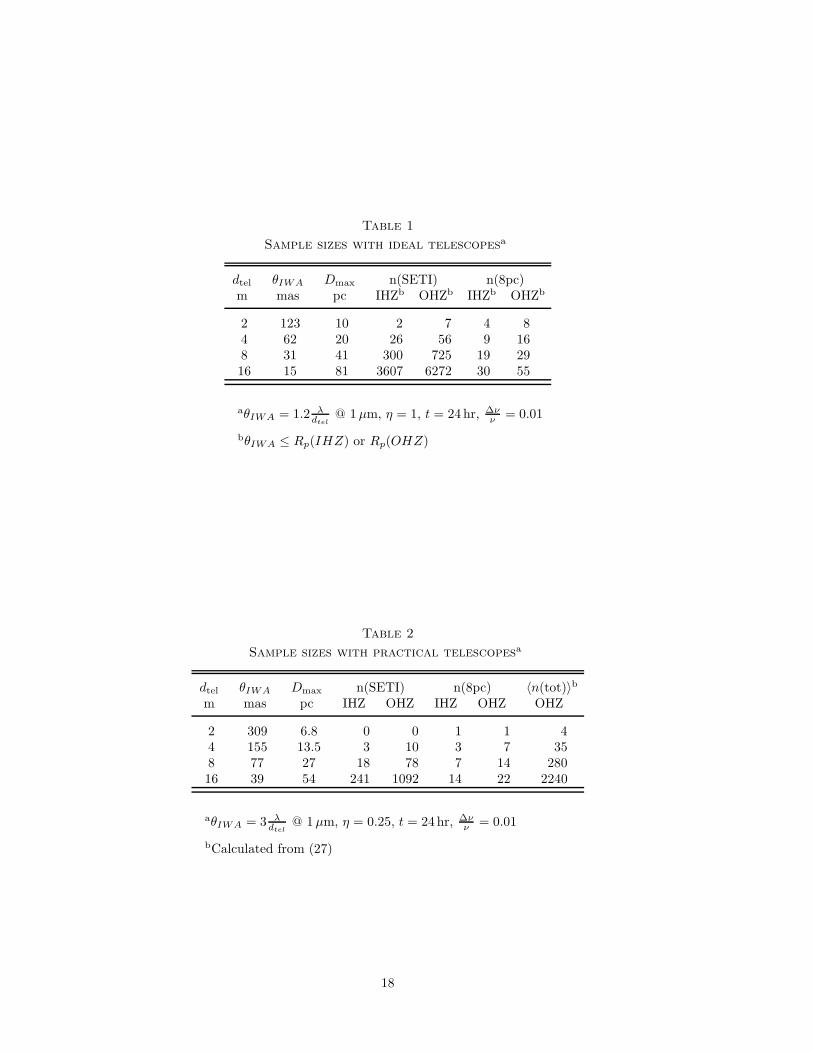
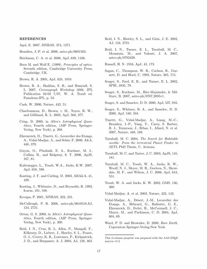
Table 1

Sample sizes with ideal telescopesa

dtel θIWA Dmax n(SETI) n(8pc)m mas pc IHZb OHZb IHZb OHZb

2 123 10 2 7 4 84 62 20 26 56 9 168 31 41 300 725 19 2916 15 81 3607 6272 30 55

aθIWA = 1.2 λdtel

@ 1 µm, η = 1, t = 24hr, ∆νν = 0.01

bθIWA ≤ Rp(IHZ) or Rp(OHZ)

Table 2

Sample sizes with practical telescopesa

dtel θIWA Dmax n(SETI) n(8pc) 〈n(tot)〉bm mas pc IHZ OHZ IHZ OHZ OHZ

2 309 6.8 0 0 1 1 44 155 13.5 3 10 3 7 358 77 27 18 78 7 14 28016 39 54 241 1092 14 22 2240

aθIWA = 3 λdtel

@ 1 µm, η = 0.25, t = 24hr, ∆νν = 0.01

bCalculated from (27)

18

Table 3

Sample sizes for transit detectionsa

dtel(m) n(SETI) n(8pc)b ntotd 〈nexpect〉e

ROHZb RIHZ

c ROHZ RIHZ Tp = T⊕ Tp = T⊕

2 0 1 3 19 8 04 3 33 22 71 62 18 40 256 75 87 500 516 284 942 87 90 4000 40

a∆ν/ν = 0.01, 10σ, 5 yr, ρ = 5.5 g cm−3, µ = 30 amu, x = 4.2

bNumbers restricted by 8 pc sample limit

cPlanet orbit at inner or outer HZ: Tp = 373 or 273K

dCalculated from (54)

3Calculated from (55)

19