Embed Size (px)
Citation preview
Fourier Analysis, Multiresolution Analysis and
Dilation Equations
David Malone
September 1997

Declaration
I do declare that:
• This wasn’t anyone’s homework.
• As work goes it’s mine, mine, all mine, ∗ and where I’ve used other peoples work I’ve
said so. †
• You know what the library can do with this when they get it? More or less whatever
they want. They should keep my name on it though.
Or — at your discretion:
• This has not previously been submitted as an exercise for a degree at this or any
other University.
• This work is my own except where noted in the text.
• The library should lend or copy this work upon request.
David Malone (May 2, 2001).
∗Keep your greasy paws off it.†So there!
i
Summary
This thesis has essentially two parts.
The first two chapters are an introduction to the related areas of Fourier analysis,
multiresolution analysis and wavelets. Dilation equations arise in the context of multires-
olution analysis. The mathematics of these two chapters is informal, and is intended to
provide a feeling for the general subject. This work is loosely based on two talks which
I gave, one during the 1997 Inter-varsity Mathematics competition and the other at the
1997 Dublin Institute for Advanced Studies Easter Symposium.
The second part, Chapters 3 and 4, contain original work. Chapter 3 provides a new
formal construction of the Fourier transform on Lp(Rn) (1 ≤ p ≤ 2) based on the ideas
introduced in Chapter 2.
The idea is to take some basic properties of the Fourier transform and show we can
construct a bounded operator on L2(R) with these properties. I do this by constructing
an operator on each level of the Haar multiresolution analysis, which I then show is well
enough behaved to be extended by a limiting process to all of L2(R).
Some of the important properties of the Fourier transform are also derived in terms of
this construction, and the generalisations to Lp(Rn) are explored.
Chapter 4 builds on the work of Chapters 3 and provides a uniqueness result for the
Fourier transform. While searching for this result I also establish a related result for
dilation equations (a subject also introduced in Chapter 2).
Here the exact set of properties which were used to define the Fourier transform are
varied in an effort to discover which are merely consistent with the Fourier transform
and which strong enough to define it. I end up examining sets of dilation equations and
determining when these will have a unique solution.
ii

Acknowledgments
I’m not really sure who I should acknowledge. When listing people you are sure to miss
people to whom credit is due and perhaps even accidently include people who have had no
real input. For instance:
I’d like to thank Elvis for all those lunchtime chats in which he tried to explain why
the “admissibility condition” wasn’t a terrible name. Also the comments Jimmi Hendrix
and Jesus made on layout were very helpful.
However, everyone seems to do their best when compiling acknowledgments, and why
should I be the exception?
I should first thank my supervisor, Richard Timoney, and other members of the School
of Mathematics who have provided me with access to a far better source of information
than books — experience. That is not to say they did not provide me with access to
books too, the library in the basement is quite comprehensively stocked. Sarah Ziesler
also performed a broad assessment of and commentary on the second half of this work —
always a useful thing.
My family and the Trinity Foundation have provided support of a very practical nature.
My family house, feed and put up with me. The Trinity Foundation have funded my time
as a postgraduate. The secretarial staff of the School of Mathematics have always provided
help with photocopying, stapling and looking over printouts before I use them.
John Lewis of DIAS and the committee of the Dublin University Mathematics Soci-
ety provided me with opportunities to address two quite different audiences. Both were
educational and enjoyable experiences.
There is a long list of people who have helped by talking through things with me,
volunteering for proof reading duty or just listening to me babble about whatever I was
thinking about at the time. This list of people includes, but is not limited to: Peter Clifford,
Shane Crowe, Ian Dowse, Ken Duffy, Eoin Hickey, Lesley Malone, Sharon Murphy, Ray
Russell, Karl Stanley and John Walsh.
iii
iv
Finally, Tim Murphy may pretend otherwise but does actually know more about LATEX
than anyone else. An invaluable mentor for all those using TEX.

Contents
1 Introducing Fourier Analysis 1
1.1 Introduction . . . . . . . . . . . . . . . . . . . . . . . . . . . . . . . . . . . 1
1.2 Fourier Series and Integrals . . . . . . . . . . . . . . . . . . . . . . . . . . 1
1.3 Lp and Convergence . . . . . . . . . . . . . . . . . . . . . . . . . . . . . . 4
1.4 Why bother with Fourier Analysis? . . . . . . . . . . . . . . . . . . . . . . 6
1.5 The Windowed Fourier Transform . . . . . . . . . . . . . . . . . . . . . . . 8
1.6 The Continuous Wavelet Transform . . . . . . . . . . . . . . . . . . . . . . 11
1.7 Conclusion . . . . . . . . . . . . . . . . . . . . . . . . . . . . . . . . . . . . 13
2 An Introduction to Multiresolution Analysis 14
2.1 Introduction . . . . . . . . . . . . . . . . . . . . . . . . . . . . . . . . . . . 14
2.2 What is MRA? . . . . . . . . . . . . . . . . . . . . . . . . . . . . . . . . . 14
2.3 Three Examples . . . . . . . . . . . . . . . . . . . . . . . . . . . . . . . . . 17
2.3.1 The Haar MRA . . . . . . . . . . . . . . . . . . . . . . . . . . . . . 17
2.3.2 Band-Limited MRA . . . . . . . . . . . . . . . . . . . . . . . . . . 19
2.3.3 Daubechies’ generating function . . . . . . . . . . . . . . . . . . . . 23
2.4 Dilation Equations . . . . . . . . . . . . . . . . . . . . . . . . . . . . . . . 24
2.4.1 Integrability . . . . . . . . . . . . . . . . . . . . . . . . . . . . . . . 24
2.4.2 Orthonormality . . . . . . . . . . . . . . . . . . . . . . . . . . . . . 25
2.4.3 Ability to Approximate . . . . . . . . . . . . . . . . . . . . . . . . . 25
2.5 Discrete Wavelets . . . . . . . . . . . . . . . . . . . . . . . . . . . . . . . . 26
2.6 Back to the examples . . . . . . . . . . . . . . . . . . . . . . . . . . . . . . 28
2.6.1 Haar Wavelets . . . . . . . . . . . . . . . . . . . . . . . . . . . . . . 29
2.6.2 Shannon Wavelets . . . . . . . . . . . . . . . . . . . . . . . . . . . . 29
2.6.3 Daubechies’ Wavelets . . . . . . . . . . . . . . . . . . . . . . . . . . 31
2.7 How to draw these beasties . . . . . . . . . . . . . . . . . . . . . . . . . . . 31
v

CONTENTS vi
2.8 Conclusion . . . . . . . . . . . . . . . . . . . . . . . . . . . . . . . . . . . . 33
3 A New Construction for the Fourier Transform 35
3.1 Introduction . . . . . . . . . . . . . . . . . . . . . . . . . . . . . . . . . . . 35
3.2 Defining F on our MRA . . . . . . . . . . . . . . . . . . . . . . . . . . . . 36
3.3 Extending F to L2(R) . . . . . . . . . . . . . . . . . . . . . . . . . . . . . 41
3.4 Back to the traditional . . . . . . . . . . . . . . . . . . . . . . . . . . . . . 43
3.5 Can we do better than that? . . . . . . . . . . . . . . . . . . . . . . . . . . 47
3.6 Extending properties of F . . . . . . . . . . . . . . . . . . . . . . . . . . . 48
3.7 The inverse Fourier transform . . . . . . . . . . . . . . . . . . . . . . . . . 50
3.8 Higher dimensions . . . . . . . . . . . . . . . . . . . . . . . . . . . . . . . 52
3.9 Lp(Rn) for other p. . . . . . . . . . . . . . . . . . . . . . . . . . . . . . . . 55
3.10 Conclusions . . . . . . . . . . . . . . . . . . . . . . . . . . . . . . . . . . . 59
4 A Uniqueness Result for the Fourier Transform 62
4.1 Introduction . . . . . . . . . . . . . . . . . . . . . . . . . . . . . . . . . . . 62
4.2 A simple start . . . . . . . . . . . . . . . . . . . . . . . . . . . . . . . . . . 63
4.3 A useful counterexample . . . . . . . . . . . . . . . . . . . . . . . . . . . . 64
4.4 How many solutions? . . . . . . . . . . . . . . . . . . . . . . . . . . . . . . 68
4.5 Some more dilation equations . . . . . . . . . . . . . . . . . . . . . . . . . 71
4.6 Pinning it down . . . . . . . . . . . . . . . . . . . . . . . . . . . . . . . . . 74
4.7 Conclusion . . . . . . . . . . . . . . . . . . . . . . . . . . . . . . . . . . . . 78
5 Future Work 79
List of Figures
1.1 Averages of cosnx . . . . . . . . . . . . . . . . . . . . . . . . . . . . . . . 2
1.2 e−x2
cos(7x) and its Fourier transform . . . . . . . . . . . . . . . . . . . . . 7
1.3 5 notes and its Fourier transform . . . . . . . . . . . . . . . . . . . . . . . 8
1.4 Possible windows for the WFT . . . . . . . . . . . . . . . . . . . . . . . . . 9
1.5 FT and WFT of 5 notes. . . . . . . . . . . . . . . . . . . . . . . . . . . . . 10
1.6 A wavelet and its Fourier Transform . . . . . . . . . . . . . . . . . . . . . 12
2.1 The approximation process. . . . . . . . . . . . . . . . . . . . . . . . . . . 15
2.2 g(x) for the Haar MRA. . . . . . . . . . . . . . . . . . . . . . . . . . . . . 18
2.3 Improving Approximations. . . . . . . . . . . . . . . . . . . . . . . . . . . 20
2.4 g(x) = sinπxπx
. . . . . . . . . . . . . . . . . . . . . . . . . . . . . . . . . . . . 21
2.5 g(x) for one of Daubechies’ MRAs. . . . . . . . . . . . . . . . . . . . . . . 23
2.6 w(x) for the Haar MRA. . . . . . . . . . . . . . . . . . . . . . . . . . . . . 29
2.7 w(x) for the Band-Limited MRA. . . . . . . . . . . . . . . . . . . . . . . . 30
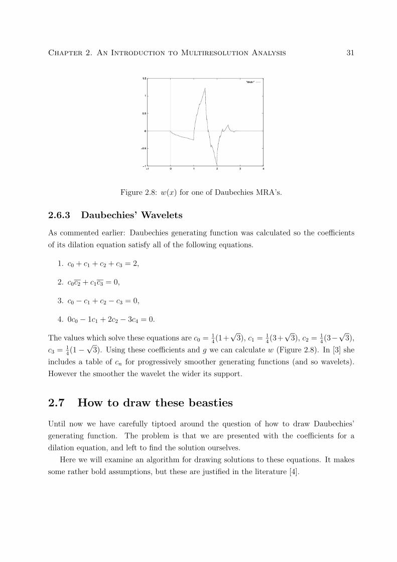
2.8 w(x) for one of Daubechies MRA’s. . . . . . . . . . . . . . . . . . . . . . . 31
2.9 C code for estimating g . . . . . . . . . . . . . . . . . . . . . . . . . . . . . 33
3.1∣∣∣1−e−iωiω
∣∣∣ . . . . . . . . . . . . . . . . . . . . . . . . . . . . . . . . . . . . . 57
4.1 φ(x) . . . . . . . . . . . . . . . . . . . . . . . . . . . . . . . . . . . . . . . 65
vii
Chapter 1
Introducing Fourier Analysis
1.1 Introduction
Fourier analysis has become an extremely useful subject in mathematics, science and en-
gineering. This section will explain the idea behind the Fourier transform and also show
how this idea leads to wavelet analysis. The emphasis here is on an intuitive understanding
and motivation for the steps taken, not a formal justification — which can be read in any
mathematical book on these subjects [15, 16]. The actual process of calculating and using
Fourier analysis is dealt with in most engineering mathematics books, for example [10].
The basic idea of Fourier analysis is: Suppose we have some function f , which we know
is a sum of terms something like an cos(nx), but we don’t know what the an are. Then
how do we find exactly what these terms are? For engineers this amounts to looking at
how much (an) of what basic frequencies (n) make up a given signal (f).
1.2 Fourier Series and Integrals
To keep the details simple we will start by looking at a ‘Fourier cosine series’. Suppose we
have some function f which we know is a sum∗ of the form:
f(x) =∑n=0
an cosnx,
∗We have deliberately left the upper limit of the sum out, as we do not want to look at the issue ofconvergence yet.
1
Chapter 1. Introducing Fourier Analysis 2
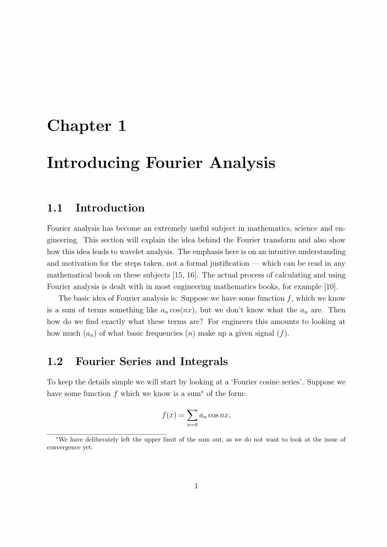
cos(0x) cos(1x) cos(2x)
Average 1 Average 0 Average 0
Figure 1.1: Averages of cosnx
but we do not know what the exact values of the an are. How do we go about finding what
these an are? There are essentially three tricks to finding the an. First, f(x) must have
period which divides 2π, because all the cosnx repeat themselves after 2π. The second
trick involves looking at the average of cosnx on [0, 2π]. Looking at Figure 1.1 we see that
cosnx has average 0 whenever n is not 0. We can exploit this by averaging f .∫ 2π
0
f(x) dx =∑n=0
an
∫ 2π
0
cosnx dx = 2πa0
So now we have found a0. We would like to be able to use the same trick to pick out the
rest of the an. This is where the third trick comes in. We look at what happens when we
multiply cosnx by cosmx:
cosnx cosmx = 1/2 (cos(m+ n)x+ cos(m− n)x)
Averaging both sides (again over [0, 2π]) we see that we get a contribution of 1/2 ifm+n = 0
and another 1/2 if n−m = 0. If we get both contributions then n = m = 0, which we have
dealt with. Otherwise we need n = m to get a contribution (because we are only worried
about n ≥ 0 at the moment).
Using what we have just learned we try multiplying f by cosmx before averaging.∫ 2π
0
f(x) cosmxdx =∑n=0
an
∫ 2π
0
cosnx cosmxdx
= πam
So now, all formalities out of the way we have found a way to determine the an given the
function f .

Chapter 1. Introducing Fourier Analysis 3
Further examination of the usual trigonometric identities lets us do some variations on
this theme. By using the formulas:
cosnx sinmx = 1/2 (sin(n+m)x− sin(n−m)x)
and
sinnx sinmx = 1/2 (cos(n−m)x− cos(n+m)x)
and also remembering that sinnx averages to zero (over [0, 2π]) regardless of the value of
n we may deal with a more general situation. This time suppose that f is expressible in
the following form:
f(x) =∑n=0
an cosnx+ bn sinnx.
By going through the process of multiplying by cosmx or sinmx and averaging we even-
tually get expressions for an and bn.
a0 =1
2π
∫ 2π
0
f(x) dx
b0 = 0 (doesn’t matter)
an =1
π
∫ 2π
0
f(x) cosmxdx
an =1
π
∫ 2π
0
f(x) sinmxdx
Naturally we can make many variants of this. The an and bn could be objects in some real
vector space, we could work on [0, 1] instead of [0, 2π] or we could just use sin. The two
most important variations are replacing trigonometric functions with einx and replacing
sums with integrals.
Replacing sin x and cosx with eix is generally viewed as a simplification. We retain the
same degree of generality (we now work with a sum from −∞ to∞) but we only need one
formula. If we suppose that:
f(x) =∞∑
n=−∞
cneinx
and remember that einx has period dividing 2π, we might be tempted to average over [0, 2π]
again. The average of einx is zero over the range [0, 2π] — unless n is 0 when the average
Chapter 1. Introducing Fourier Analysis 4
is 1. This combined with the fact:
einxeimx = ei(n+m)x,
means that f(x)e−imx has mean cm over [0, 2π]. So we get a simple expression for the cm:
cm =1
2π
∫ 2π
0
f(x)e−imx dx.
Now we attempt to replace our sums with integrals. This requires a certain extra leap
of faith as regards convergence. If we believe that in some sense eiωx has average 0 for all
ω ∈ R \ 0 then we can hope that if:
f(x) =
∫ ∞−∞
c(ω)eiωx dω,
then there is some chance that:
c(ω) =1
2π
∫ ∞−∞
f(x)e−iωx dx.
In this case c(ω) is called the Fourier transform of f . As we can see there is a certain
degree of symmetry in the expressions for f and c. For this reason people often move
around factors of 2π or√
2π to try to make the situation even more symmetric.
The next two questions that arise are: what functions can we write in these forms,
and where don’t we have to worry about convergence problems? The answers to these
questions are related, and the relation is linked to the symmetry we have just noted.
1.3 Lp and Convergence
When looking at the convergence of something like:∫ ∞−∞
f(x)e−iωx dx,
for various values of ω the first thing we can note is that |e−iωx| = 1, so all we really need
to worry about is: ∫ ∞−∞
f(x) dx.

Chapter 1. Introducing Fourier Analysis 5
However, we may as well just look at |f | because it might turn out that f was strictly
positive, or that multiplying f by e−iωx made it strictly positive. This leaves us looking at:∫ ∞−∞|f(x)| dx.
This is called the L1 norm of f and is usually written ‖f‖1. On the set of f where ‖f‖1 is
finite (this is called L1(R)), this ‖.‖1 is a norm in the usual normed vector space sense —
barring some complications regarding equivalence classes.
On this space, L1(R), we find the Fourier transform is quite well behaved. It is rea-
sonably easy to show that if f is in L1(R) then its Fourier transform is a continuous and
bounded function of ω. However this doesn’t really reflect the symmetry we noticed. We
started with L1(R), applied the Fourier transform and got continuous and bounded func-
tions. The symmetry would suggest that we search for a space which the Fourier transform
sends to itself. Here, perhaps, the Fourier transform might even be invertible.
A similar norm to ‖.‖1, but one closer to the traditional Euclidean norm would be:
‖f‖2 =
√∫ ∞−∞|f(x)|2 dx.
We call the space of functions where this new norm is finite L2(R). Again, ignoring some
complications with equivalence classes of functions, this is also a normed vector space. It
also turns out to be the ideal space for Fourier analysis. It can be shown (though it takes
some work) that the Fourier transform is a linear, continuous and invertible transform,
both to and from this normed vector space: L2(R).
When looking at Fourier series and other problems we can generalise our definition of
spaces of this sort. A few examples best illustrate the idea.
L1(R) =
f : R→ C|
∫ ∞−∞|f(x)| dx <∞
L2([0, 2π]) =
f : [0, 2π]→ C|
∫ 2π
0
|f(x)|2 dx <∞
L3(N) =
an ∈ C|n ∈ N,
∞∑n=0
|an|3 <∞
The first example we have already seen. The second relates to the Fourier series for 2π
periodic functions. The last gives an example of other sorts of Lp type spaces which we

Chapter 1. Introducing Fourier Analysis 6
can consider. In general for X a set† with a positive measure µ we could define Lp(X,µ)
to be the set: f : X → C|f measurable and
∫X
|f |p dµ <∞
In this context our third example was no more than this general definition on N with the
counting measure. This family Lp(N, counting) is often just written lp, as they are rather
commonly encountered spaces.
1.4 Why bother with Fourier Analysis?
Fourier analysis (which is this process of writing things in terms of einx), has some good
reasons for being of interest. Naturally all these reasons are interlinked. We’ll start from
a mathematical reason and then work toward a practical reason.
One of the important topics which mathematicians deal with is the study of differential
equations. If we look at v(x) = eiωx, then we see that v is an eigenvector for differentiation.
That is:d
dxv =
d
dx
(eiωx
)= iωeiωx = iωv.
So differentiating v has a very simple effect on it (it gets multiplied by iω). If we are looking
for a solution of some differential equation and we know the solution may be expressed as
the sum (or integral) of terms like eiωx then, the differential equation should have a simple
form for each of these terms, which will hopefully be easy to solve. This means that Fourier
analysis is likely to be useful for solving physical problems, which often involve differential
equations.
An important differential equation which lends itself to this sort of Fourier analysis
perfectly is the wave equation.∂2
∂x2− 1
c2
∂2
∂t2= 0
This equation describes many things, including the transmission of electromagnetic waves
(light) and sound. For this reason Fourier analysis is of great interest to engineers working
with light or sound signals. They think of the Fourier transform of a signal as showing
“how much” of each frequency is in a signal. Also, in this analogy, the ‖.‖22 corresponds to
the energy of the signal, making results easy to interpret.
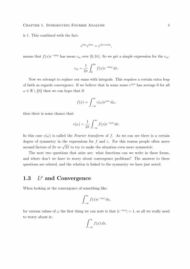
An example may make this clearer. In Figure 1.2 we see a signal which we would expect
†More technically, we need a measure space rather than just a set.
Chapter 1. Introducing Fourier Analysis 7
Figure 1.2: e−x2
cos(7x) and its Fourier transform
to be mostly composed of a wave of angular frequency 7 (as it is mainly cos 7x). If we look
at its Fourier transform we see that there is a large peak near 7, as we would have hoped.
A more complicated example reveals both the strength and weakness of this sort of
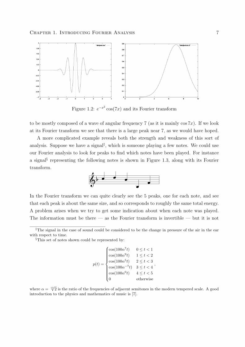
analysis. Suppose we have a signal‡, which is someone playing a few notes. We could use
our Fourier analysis to look for peaks to find which notes have been played. For instance
a signal§ representing the following notes is shown in Figure 1.3, along with its Fourier
transform.
G2 In the Fourier transform we can quite clearly see the 5 peaks, one for each note, and see
that each peak is about the same size, and so corresponds to roughly the same total energy.
A problem arises when we try to get some indication about when each note was played.
The information must be there — as the Fourier transform is invertible — but it is not
‡The signal in the case of sound could be considered to be the change in pressure of the air in the earwith respect to time.§This set of notes shown could be represented by:
p(t) =
cos(100α7t) 0 ≤ t < 1cos(100α9t) 1 ≤ t < 2cos(100α5t) 2 ≤ t < 3cos(100α−7t) 3 ≤ t < 4cos(100α0t) 4 ≤ t < 50 otherwise
,
where α = 12√
2 is the ratio of the frequencies of adjacent semitones in the modern tempered scale. A goodintroduction to the physics and mathematics of music is [7].
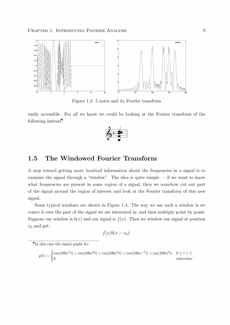
Chapter 1. Introducing Fourier Analysis 8
Figure 1.3: 5 notes and its Fourier transform
easily accessible. For all we know we could be looking at the Fourier transform of the
following instead¶.
G2
1.5 The Windowed Fourier Transform
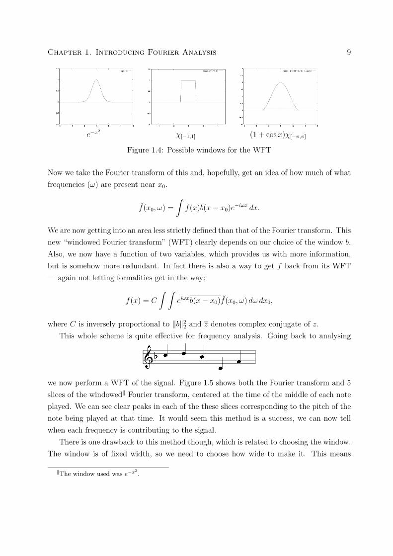
A step toward getting more localised information about the frequencies in a signal is to
examine the signal through a “window”. The idea is quite simple — if we want to know
what frequencies are present in some region of a signal, then we somehow cut out part
of the signal around the region of interest and look at the Fourier transform of this new
signal.
Some typical windows are shown in Figure 1.4. The way we use such a window is we
center it over the part of the signal we are interested in, and then multiply point by point.
Suppose our window is b(x) and our signal is f(x). Then we window our signal at position
x0 and get:
f(x)b(x− x0).
¶In this case the signal might be:
p(t) =
cos(100α7t) + cos(100α9t) + cos(100α5t) + cos(100α−7t) + cos(100α0t) 0 ≤ t < 10 otherwise
.
Chapter 1. Introducing Fourier Analysis 9
e−x2
χ[−1,1] (1 + cos x)χ[−π,π]
Figure 1.4: Possible windows for the WFT
Now we take the Fourier transform of this and, hopefully, get an idea of how much of what
frequencies (ω) are present near x0.
f(x0, ω) =
∫f(x)b(x− x0)e−iωx dx.
We are now getting into an area less strictly defined than that of the Fourier transform. This
new “windowed Fourier transform” (WFT) clearly depends on our choice of the window b.
Also, we now have a function of two variables, which provides us with more information,
but is somehow more redundant. In fact there is also a way to get f back from its WFT
— again not letting formalities get in the way:
f(x) = C
∫ ∫eiωxb(x− x0)f(x0, ω) dω dx0,
where C is inversely proportional to ‖b‖22 and z denotes complex conjugate of z.
This whole scheme is quite effective for frequency analysis. Going back to analysing
G2 we now perform a WFT of the signal. Figure 1.5 shows both the Fourier transform and 5
slices of the windowed‖ Fourier transform, centered at the time of the middle of each note
played. We can see clear peaks in each of the these slices corresponding to the pitch of the
note being played at that time. It would seem this method is a success, we can now tell
when each frequency is contributing to the signal.
There is one drawback to this method though, which is related to choosing the window.
The window is of fixed width, so we need to choose how wide to make it. This means
‖The window used was e−x2.

Chapter 1. Introducing Fourier Analysis 10
Centered at 0.5 Centered at 1.5 Centered at 2.5
Centered at 3.5 Centered at 4.5
Figure 1.5: FT and WFT of 5 notes.

Chapter 1. Introducing Fourier Analysis 11
we must either know the length of the “notes” of interest within the signal or we must
experiment until we find a good width. If we make the window too narrow we will be
unable to look at signals with a wavelength much longer than this width. If we make the
window too wide we blur adjacent notes together.
For Figure 1.5 the window chosen had a width on the same scale as the length of the
notes (we can actually see the adjacent notes as smaller peaks, so it may have been a little
too wide). Trying to remove this limitation of the WFT leads us to the continuous wavelet
transform.
1.6 The Continuous Wavelet Transform
The problem with the windowed Fourier transform is that the window is of fixed width.
The correct direction to move in would seem to involve varying the width of the window.
However if we just introduce a new parameter for window width, then we have a 3 parameter
transform (ω for frequency, x0 for position and say w for width), which some might view
as getting a wee bit out of hand.
Realising that the width of the window can be related to the frequency which we are
looking for is a useful trick. The shortest burst of some frequency that can be easily
identified as being of that frequency is about half a wavelength∗∗ of said frequency. So if
we choose a window width of about this length then we stand a good chance of picking up
on that frequency.
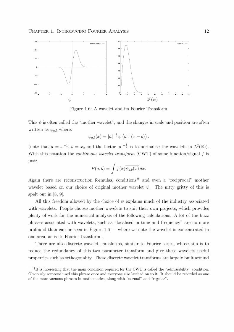
So what we do is choose a window (say e−x2) and a wave (say sinx), and glue them
together to get a wavelet.
ψ(x) = e−x2
sin x
Now, in the same way as with the WFT, we center our wavelet over the signal.
ψ(x− x0) = e−(x−x0)2
sin(x− x0)
We also note that if we want to search for frequency ω we just scale the whole thing by ω,
as this produces a sinωx which will hopefully pick up on this frequence.
ψ (ω(x− x0)) = e−ω2(x−x0)2
sinω(x− x0)
∗∗This can be made more formal, by Shannon’s sampling theorem, see Theorem 2.1.
Chapter 1. Introducing Fourier Analysis 12
ψ F(ψ)
Figure 1.6: A wavelet and its Fourier Transform
This ψ is often called the “mother wavelet”, and the changes in scale and position are often
written as ψa,b where:
ψa,b(x) = |a|−12ψ(a−1(x− b)
).
(note that a = ω−1, b = x0 and the factor |a|− 12 is to normalise the wavelets in L2(R)).
With this notation the continuous wavelet transform (CWT) of some function/signal f is
just:
F (a, b) =
∫f(x)ψa,b(x) dx.
Again there are reconstruction formulas, conditions†† and even a “reciprocal” mother
wavelet based on our choice of original mother wavelet ψ. The nitty gritty of this is
spelt out in [8, 9].
All this freedom allowed by the choice of ψ explains much of the industry associated
with wavelets. People choose mother wavelets to suit their own projects, which provides
plenty of work for the numerical analysis of the following calculations. A lot of the buzz
phrases associated with wavelets, such as “localised in time and frequency” are no more
profound than can be seen in Figure 1.6 — where we note the wavelet is concentrated in
one area, as is its Fourier transform .
There are also discrete wavelet transforms, similar to Fourier series, whose aim is to
reduce the redundancy of this two parameter transform and give these wavelets useful
properties such as orthogonality. These discrete wavelet transforms are largely built around
††It is interesting that the main condition required for the CWT is called the “admissibility” condition.Obviously someone used this phrase once and everyone else latched on to it. It should be recorded as oneof the more vacuous phrases in mathematics, along with “normal” and “regular”.
Chapter 1. Introducing Fourier Analysis 13
a structure called multiresolution analysis (or multiscale analysis), a subject we will come
back to in Chapter 2.
1.7 Conclusion
Here we have seen a little of Fourier analysis, a subject of interest to those involved with
either pure or applied mathematics. We have dealt mostly with why it might be of interest
to someone from a practical point of view, and said only little about the theory.
The most important result that we have missed is to do with relating the Fourier
transform of a product of two functions to their individual Fourier transforms. This result
involves the convolution of two functions:
(f ∗ g)(x) =
∫f(t)g(x− t) dt.
It states that the Fourier transform of a product is the convolution of the Fourier transforms
(up to factors of√
2π). Varying degrees of detail about this can be found in [15, 16, 10, 8].
On the practical side of things, the next most important result is probably the “Fast
Fourier Transform”, or FFT for short. This is a way of numerically calculating a Fourier
transform from a set of sampled data far more quickly than just using numerical integration.
This caused quite a stir when it came to light in the numerical world, as it changed an N2
operation into a N log2 N operation. Two whole chapters on implementation and usage of
this can be found in [13].
On the theoretical side Fourier analysis has progressed in many directions. The defi-
nition of the Fourier transform can be extended to a large class of groups. Through this
Fourier analysis has links with group representations. Many of the essays in [2] provide
summaries of or introductions to these topics. There are also links with the theory of dis-
tributions and with the study of certain types of operators on spaces where we can use the
Fourier transform. The Hilbert transform is probably the best known of these operators.
We have also looked at some practical variants of the Fourier transform, which has led
us to the continuous wavelet transform. We will be moving on to look at how a stronger
structure can be placed on these wavelet ideas to produce the discrete wavelet transform.
These wavelet transforms have attracted similar attention to the attention received by the
FFT when it appeared.

Chapter 2
An Introduction to Multiresolution
Analysis
2.1 Introduction
In this section we will be introduced to some ideas relating to the discrete wavelet transform.
The most important idea is that of a multiresolution analysis. Multiresolution analyses lead
in a natural way to dilation equations — which feature strongly in many of the following
sections. Also dilation equations lead us through the construction of the discrete wavelet
transform.
2.2 What is MRA?
Multiresolution analysis could have several names applied to it, and indeed often does.
The names multiscale analysis and multiresolution approximation are pseudonyms which
provide further hints as to what it is all about. Maybe one of the more intuitive ways to
approach MRA is from the approximation side.
When we want to approximate something we usually take several steps.
1. First we choose some function with which we will approximate. Maybe a spline of
some sort, maybe something specially tailored for our approximation problem.
2. We translate our chosen function to various nodes, where each translated function
will do its approximation. Often these nodes might be the integers.
3. We multiply each translated function by some carefully chosen coefficients.
14
Chapter 2. An Introduction to Multiresolution Analysis 15
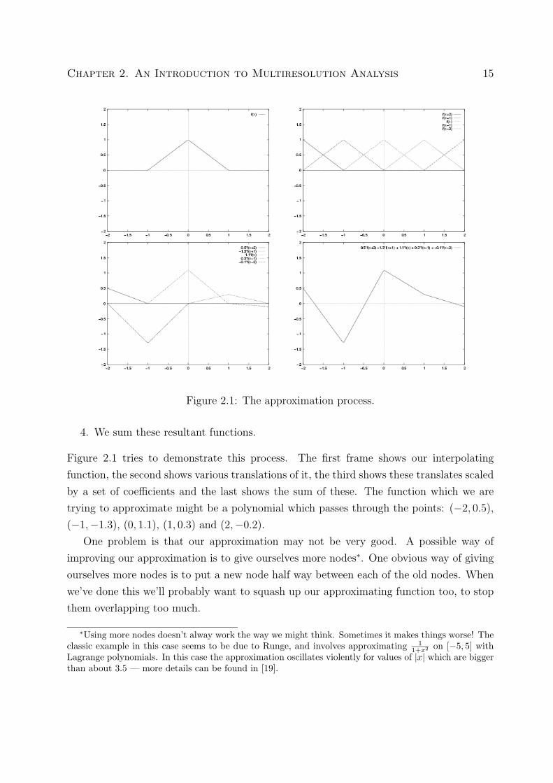
Figure 2.1: The approximation process.
4. We sum these resultant functions.
Figure 2.1 tries to demonstrate this process. The first frame shows our interpolating
function, the second shows various translations of it, the third shows these translates scaled
by a set of coefficients and the last shows the sum of these. The function which we are
trying to approximate might be a polynomial which passes through the points: (−2, 0.5),
(−1,−1.3), (0, 1.1), (1, 0.3) and (2,−0.2).
One problem is that our approximation may not be very good. A possible way of
improving our approximation is to give ourselves more nodes∗. One obvious way of giving
ourselves more nodes is to put a new node half way between each of the old nodes. When
we’ve done this we’ll probably want to squash up our approximating function too, to stop
them overlapping too much.
∗Using more nodes doesn’t alway work the way we might think. Sometimes it makes things worse! Theclassic example in this case seems to be due to Runge, and involves approximating 1
1+x2 on [−5, 5] withLagrange polynomials. In this case the approximation oscillates violently for values of |x| which are biggerthan about 3.5 — more details can be found in [19].
Chapter 2. An Introduction to Multiresolution Analysis 16
Essentially this is all there is to multiresolution analysis. Giving ourselves new nodes
is a change of resolution and squashing our functions is a change of scale. Multiresolution
analysis studies what happens when we vary this scale.
Now for the formal definition of multiresolution analysis.
Definition 2.1. A multiresolution analysis of L2(R) is a collection of subsets Vjj∈Z of
L2(R) such that:
1. ∃ g ∈ L2(R) so that V0 consists of all (finite) linear combinations of g(x−k) : k ∈ Z,
2. the g(x− k) are an orthonormal † series in V0,
3. f(x) ∈ Vj ⇐⇒ f(2x) ∈ Vj+1‡,
4.+∞⋃j=−∞
Vj is dense in L2(R),
5.+∞⋂j=−∞
Vj = 0,
6. Vj ⊂ Vj+1.
We may think of g as our chosen approximating function. V0 contains all the functions
we can make by adding up translations of g to the integers. When we give ourselves twice
as many nodes and squash our generating function we move from Vj to Vj+1. Condition 4
means we can approximate any L2(R) function as closely as we choose. Condition 6 ensures
that our approximation is improving all the time: it would be a bit unfortunate if we got
to V10 and had the exact function we wanted only to find it wasn’t in V11.
Some authors leave out the orthogonality requirement (condition 2). They then refer
to a multiresolution analysis with this extra property as an orthogonal multiresolution
analysis. This would be somewhat clearer, and leave the definition usable on spaces where
we do not have the idea of things being orthogonal (for example in Lp(R) for most p).
However the majority of authors do include condition 2.
†We say 2 functions f and g are orthogonal if∫f(x)g(x) dx = 0. This parallels two vectors ~x, ~y being
orthogonal if∑xiyi = 0. We say a series is orthonormal if the members are pairwise orthogonal and
‖f‖2 = 1 for each f in the sequence.‡This notation is bad — what we really mean is: f(.) ∈ Vj ⇐⇒ f(2.) ∈ Vj+1. We will, however, stick
with the bad notation, as it seems more natural.

Chapter 2. An Introduction to Multiresolution Analysis 17
One obvious way to construct an MRA is to pick a g and to produce V0 using rule 1.
Then form Vj using rule 3 and applying rule 4 we, hopefully, get all of L2(R). We do
then have to check that the g which we chose will be orthogonal to its translates, that the
intersection of the Vj contains only zero and that Vj ⊂ Vj+1.
We can easily extend this definition to L2(Rn) for any n. We just replace L2(R) with
L2(Rn) throughout the definition and substitute g(x−k) : k ∈ Z with g(x−k) : k ∈ Znin condition 1.
2.3 Three Examples
We’ll take a look at a few examples which demonstrate a few of the forms a multiresolution
analysis can take, and also some possible applications. The first example is the classical
example of the Haar multiresolution analysis. This is more or less the canonical multires-
olution analysis, and can be kept in mind when dealing with almost any property of a
multiresolution analysis.
The second example deals with functions whose Fourier transform is zero outside a
given range. It is an interesting MRA because it is easy to describe without defining it
in terms of its generating function. Functions whose Fourier transforms are zero outside a
given interval are often called band-limited.
The last example is generated by one of Daubechies’ generating functions. This example
is of interest because it leads to “compactly supported smooth orthogonal wavelets”, which
are one of the most touted achievements of the theory of wavelets.
The first two examples are discussed in significant brevity at the beginning of the second
chapter of [12], and in [9] in the “Wavelets and Multiresolution Analysis” chapter. Perhaps
one of the best references for the third example is the often cited original paper [3], but
most introductions [17, 8] to the topic of wavelets will at least mention it.
2.3.1 The Haar MRA
To form the Haar MRA we begin by taking g to be:
g(x) =
1 x ∈ [0, 1)
0 otherwise.

Chapter 2. An Introduction to Multiresolution Analysis 18
Figure 2.2: g(x) for the Haar MRA.
This is commonly known as the indicator or characteristic function of the set [0, 1), and
is usually written χ[0,1)(x). In this case the translates of g are the characteristic functions
of the intervals [n, n+ 1) for each of the integers n, which are quite clearly orthogonal (as
their supports§ do not even overlap).
We now make V0 the set of finite linear combinations of these characteristic functions,
so V0 will just contain functions which are piecewise constant on each interval [n, n + 1)
and have compact support.
We look at what V1 is going to be. Using f(x) ∈ V0 ⇐⇒ f(2x) ∈ V1, we find ourselves
looking at g(2x), which turns out to be the same as χ[0, 12
)(x). Following from this we find
V1 will contain functions which are constant on [n/2, n/2 + 1/2) where n ∈ Z. If we repeat
this process we find:
Vj =
f : f has compact support and piecewise constant on
[n
2j,n+ 1
2j
)∀n ∈ Z
.
As any function which is constant on[n2j, n+1
2j
)is certainly constant on
[2n
2j+1 ,2n+12j+1
),
these spaces are nested.
How do we show the union of these Vj is dense in L2(R)? Well, this union contains
step functions whose steps change height at n2−j for n, j ∈ Z. These functions are dense
in the set of all step functions, which in turn are dense in L2(R).
The intersection of all these Vj will contain functions which are constant on intervals
of the form [n2−j, (n+ 1)2−j), and which are in L2(R). In particular by looking at n = 0
§The support of a function is the closure of the set where is nonzero.

Chapter 2. An Introduction to Multiresolution Analysis 19
and n = 1 we see the functions are constant on [0, 2−j) and [−2−j, 0) for any j ∈ Z. This
means that these functions are constant on [0,∞) and (−∞, 0). But the only function in
L2(R) which is constant on all such large intervals is the constant zero function.
This multiresolution analysis might be said to consist of functions which are constant
on dyadic intervals. A dyadic number is one of the form n2−j with n, j ∈ Z. Dyadic
intervals are intervals with these numbers as end points.
In L2(R2) we could use a similar construction, this time starting with g to be the char-
acteristic function of the unit square [0, 1)× [0, 1). In this case we’ll get a multiresolution
analysis of functions constant on dyadic squares. This naturally generalises to L2(Rn).
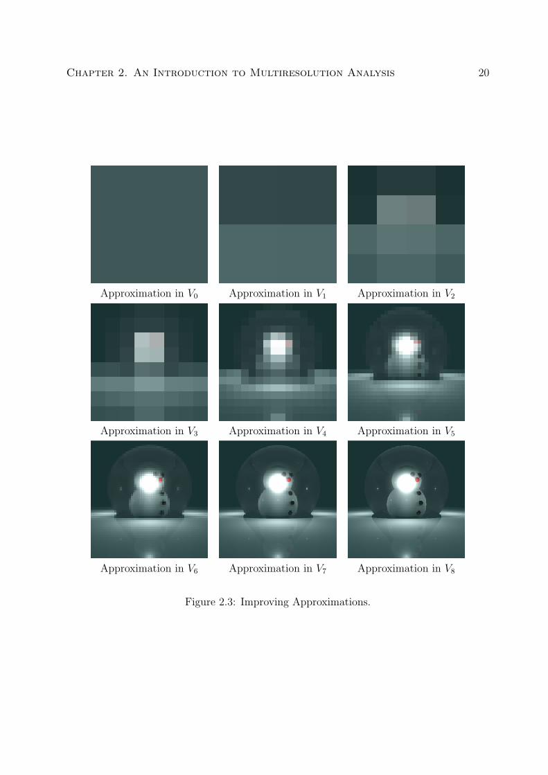
Figure 2.3 shows an example of how approximations converge to an function on R2. As
this example suggests multiresolution has been applied to various sorts of image analysis.
Indeed “mip-mapping” used in image rendering is very similar in structure to this MRA
([22] page 141 and plate 4).
2.3.2 Band-Limited MRA
In this example we start by defining the sets Vj.
Vj =f ∈ L2(R) : f is supported on [−2jπ, 2jπ].
Here f is the Fourier transform of f , which we’ll take with the normalisation:
f(ω) =
∫ ∞−∞
e−iωxf(x) dx.
We will also use the notation F(f) for the Fourier transform of f .
One thing is clear, that as j gets bigger so does Vj, and Vj ⊂ Vj+1. Also the fact
that the union of these sets is dense in L2(R) and that the intersection only contains the
constant zero function is reasonably clear from the definition of Vj and the fact that F is
both invertible and linear.
To verify that f(x) ∈ Vj ⇐⇒ f(2x) ∈ Vj+1, we need to look at how F(f(x)) compares
to F(f(2x)). We do the calculation, and use the change of variable x′ = 2x half way
through.
F(f(2x))(ω) =
∫ ∞−∞
e−iωxf(2x) dx =1
2
∫ ∞−∞
e−iωx′2 f(x′) dx′ =
1
2F(f(x))(ω/2)
Chapter 2. An Introduction to Multiresolution Analysis 20
Approximation in V0 Approximation in V1 Approximation in V2
Approximation in V3 Approximation in V4 Approximation in V5
Approximation in V6 Approximation in V7 Approximation in V8
Figure 2.3: Improving Approximations.

Chapter 2. An Introduction to Multiresolution Analysis 21
Figure 2.4: g(x) = sinπxπx
.
From this we can see that if F(f(x)) is supported on [a, b] then F(f(2x)) is supported on
[2a, 2b]. This is exactly what we need to show f(x) ∈ Vj ⇐⇒ f(2x) ∈ Vj+1.
Finding a suitable g requires a similar sort of trickery, and is only a little more subtle.
This time we need to find out what happens to the Fourier transform as we move from
g(x) to g(x− n).
F(g(x− n))(ω) =
∫ ∞−∞
e−iωxg(x− n) dx =
∫ ∞−∞
e−iω(x′+n)g(x′) dx
= e−iωn∫ ∞−∞
e−iωx′g(x′) dx = e−iωnF(g(x))(ω)
This time using the change of variable x′ = x− n.
We need¶ linear combinations of these e−iωng(ω) to span F(V0), which contains all the
functions supported on [−π, π]. Now, by considering F(V0) as L2([−π, π]) and using what
we already know about Fourier analysis we can get these functions by taking sums of einω
with n ∈ Z. So we just have to multiply by χ[−π,π] to kill off anything outside this interval.
But this option is open to us! Suppose g has a Fourier transform which is a constant
multiple of χ[−π,π]. Then, from the change of variable formula above, we know the Fourier
transform of g(x − n) is just going to be that constant times e−iωn on [−π, π] and zero
elsewhere.
It turns out that g(x) = sinπxπx
is a g with this property, and what we have been
¶What we really want is translations of g to span V0, however the invertibility and linearity of F makethis the same as e−iωng(ω) spanning F(V0)
Chapter 2. An Introduction to Multiresolution Analysis 22
considering is a special version of Shannon’s Sampling Theorem, which says the following.
Theorem 2.1. Let f be a band-limited function, with its Fourier transform supported on
[Ω/2,Ω/2]. If ∆ is chosen so that:
∆ ≤ π
Ω,
then f may be reconstructed exactly from the samples fn = f(n∆) (for n ∈ Z) by:
f(x) =∞∑
n=−∞
fnsin π(∆−1x− n)
π(∆−1x− n).
Proof. One proof, not too far from the way we arrived at g ourselves, is found as Theo-
rem 5.1 of [8], however Kaiser’s definition of the Fourier transform is slightly different to
ours.
Let us review the situation. We have been checking this multi-resolution analysis
against Definition 2.1. We decided that conditions 6, 5 and 4 were quite believable after
examining the definition of Vj. Looking at the relationship between F(f(x)) and F(f(2x))
provided us with what we needed to check condition 3, and Shannon’s theorem provided
us with a g for condition 1.
This leaves us with only condition 2 to check. It would be reasonable to tackle this
problem head on and check:∫g(x)g(x−m) dx =
∫sin πx
πx
sin π(x−m)
π(x−m)dx = 0,
when m 6= 0. However, using another important result from Fourier analysis we can get
the result in a simpler manner.
Theorem 2.2. For f, g ∈ L2(R):∫f(x)g(x) dx = 2π
∫f(ω)g(ω) dω.
Proof. Almost any book on Fourier analysis will have a proof of this, again [8] provides a
discussion of this in section 1.4, but a more theoretical (and terse) discussion can be found
in [16] chapter 1, section 2.
This result is know as Plancherel’s theorem (as are several of its variants). It transforms

Chapter 2. An Introduction to Multiresolution Analysis 23
Figure 2.5: g(x) for one of Daubechies’ MRAs.
our orthogonality problem into checking:∫ π
−πeiωm = 0,
when m 6= 0, which is easy.
In summary, from this example, we have learned a little more about Fourier analysis,
and have seen a little of how the structure of a multiresolution analysis interacts with
Fourier analysis. It might also make us wonder at all the strange shapes and sizes a
multiresolution analysis could take.
2.3.3 Daubechies’ generating function
Figure 2.5 shows a rather strange looking function. This function was engineered by
Daubechies to have certain properties. It is compactly supported (on [0, 3]), bounded and
generates an MRA which — in some ways — is a near relation of the Haar MRA. Most
interestingly both f(x) = 1 and f(x) = x can be expressed as a sum of this function’s
translates — in much the same way as constant functions can be expressed as a sum of
the Haar generating function. Consequently this MRA is suitable for the approximation
of piecewise linear functions.
Daubechies actually produced a whole family of these generating functions, each smoother
than the previous, each supported on a larger interval [0, 2N − 1] and able to approximate
1, x, . . . , xN−1. The key to producing these generating functions was the dilation equation.
These dilation equations in turn lead to a formula for wavelets for the discrete wavelet
Chapter 2. An Introduction to Multiresolution Analysis 24
transform.
2.4 Dilation Equations
While searching for generating functions for a multiresolution analysis it is natural to ask
if there are some conditions imposed on the generating function by the structure of the
multiresolution analysis. One of the most interesting conditions comes from considering
part 6 of the MRA definition — it says V0 ⊂ V1, which means:
g ∈ V0 ⊂ V1 = span g(2x− n) : n ∈ Z .
From this we can conclude that:
g(x) =∑n∈Z
cng(2x− n).
This type of equation, where g is expressed in terms of dilated versions of itself, has been
called a dilation equation, a two scale difference equation or even a multiscale difference
equation. Solutions to this type of equation are often called scaling functions and so the
generating function of an MRA is sometimes referred to as the scaling function.
It turns out a lot can be learned about g by examining these coefficients cn. Conversely
by choosing the coefficients carefully we may be able to find a g with certain desirable
properties. We will now have a look at how some properties relate to the coefficients.
2.4.1 Integrability
If we suppose that g is integrable (ie. that is in L1(R)) we can integrate over both sides of
the dilation equation: ∫R
g(x) dx =
∫R
∑n∈Z
cng(2x− n) dx
=∑n∈Z
cn
∫R
g(2x− n) dx
=∑n∈Z
cn1
2
∫R
g(x) dx.
Chapter 2. An Introduction to Multiresolution Analysis 25
Now, providing g(x) does not have mean zero, we may divide by∫g(x) dx to get:
2 =∑n∈Z
cn.
Note that if∫g(x) dx diverges we do not get this condition on the cn.
2.4.2 Orthonormality
All these conditions use similar tricks — this time we begin with the requirement that g(x)
and g(x− n) be orthonormal, and then we fill∑cng(2x− n) in for g(x).
δ0m =
∫R
g(x)g(x−m) dx
=
∫R
(∑k∈Z
ckg(2x− k)
)(∑l∈Z
clg(2x− l)
)dx
=∑k∈Z
∑l∈Z
ckcl
∫R
g(2x− k)g(2x− l) dx
=∑k∈Z
∑l∈Z
ckcl1
2
∫R
g(x)g(x+ k − l + 2m) dx
=1
2
∑k∈Z
∑l∈Z
ckclδ0 k−l+2m
=1
2
∑k∈Z
ckck+2m
This condition, like the integrability condition, is necessary but may not be sufficient.
2.4.3 Ability to Approximate
Strang, in Appendix 2 of [18], lists the following condition:∑k∈Z
ck(−1)kkm = 0 for m = 0, 1, . . . , p− 1.
It has the following following amazing consequences:
1. The polynomials 1, x, . . . , xp−1 are linear combinations of g(x− n).
2. Smooth functions can be approximated with error of O(2−pj‖f (p)‖) in Vj.

Chapter 2. An Introduction to Multiresolution Analysis 26
3. The wavelets we will construct will be orthogonal to 1, x, . . . , xp−1. That is:∫xmw(x) dx = 0 for m = 0, 1, . . . , p− 1.
This integral is sometimes called the mth moment of w.
Proof of these consequences is related to a general theory of approximation by translates
developed for the finite element method. The “Strang-Fix” condition relates the goodness
of approximation to the degree of the zeros of the Fourier transform of g. This Strang-Fix
condition, when applied to the Fourier transform of our dilation equation, produces the
condition on the cn above.
This condition is also mentioned in [5] as being important for the convergence of various
schemes for calculating g.
Daubechies’ generating function is the unique integrable function which satisfies the
Integrability, the Orthonormality and the first 2 approximation conditions (with m = 0, 1).
2.5 Discrete Wavelets
Having dealt with dilation equations we are now in a position to build ourselves a discrete
wavelet basis for L2(R). Suppose we are working in some multiresolution analysis, and we
are trying to approximate f ∈ L2(R). Say that fj is the best approximation to f in Vj.
As we move from Vj to Vj+1 our approximation must improve — or at worst stay the
same. We can think of this as:
fj+1 = fj(x) + dj(x),
where dj is the extra detail needed to bring our approximation up to the standard in Vj+1.
Looking at this in a more general context, we might think that:
Vj+1 = Vj ⊕Wj,
where the space Wj contains all the details necessary to improve Vj, but is also orthogonal
to Vj. Then:
V0 ⊕W1 ⊕W2 ⊕W3 ⊕ · · ·

Chapter 2. An Introduction to Multiresolution Analysis 27
will be dense in L2(R). In fact, in L2(R):
∞⊕j=−∞
Wj
is dense.
Now, the neatness of this scheme becomes apparent when we remember that: f(x) ∈Vj ⇐⇒ f(2x) ∈ Vj+1. This allows us to form the same relationship between the Wj as
we have between the Vj. If we could also produce a generating function w for W0 as we
produced a g for V0 then family Wj would have a very neat form indeed.
As luck would have it,
w(x) =∑k∈Z
(−1)kc1−kg(2x− k)
is just such a function! We can certainly see that this w is in V1, as it is the sum of
translates of g(2x). We can also check it is not in V0 by showing that it is orthogonal to
all translates of g(x).
∫R
g(x− n)w(x) dx =
∫R
(∑l∈R
clg(2x− l − 2n)
)(∑k∈Z
(−1)kc1−kg(2x− k)
)dx
=∑k∈Z
∑l∈R
(−1)kc1−kcl
∫R
g(2x− l − 2n)g(2x− k) dx
=∑k∈Z
∑l∈R
(−1)kc1−kclδk l+2n as translates are orthonormal
=∑k∈Z
(−1)kc1−kck−2n
=∑k∈Z
c1−2kc2k−2n −∑k∈Z
c−2kc2k−2n+1 separating even and odd
=∑k∈Z
c1−2kc2k−2n −∑l∈Z
c2l−2nc1−2l
= 0
The last step is performed by changing dummy variable to l so that 2k − 2n+ 1 = 1− 2l.
So we know that w(x) is in V1 and orthogonal to all of V0, so it seems very likely that
w is the required function. For the full proof see [12] Chapter 3 Theorem 1 or the chapter

Chapter 2. An Introduction to Multiresolution Analysis 28
of [9] entitled “Discrete Wavelets and Multiresolution analysis” Theorem 5.1‖.
This w(x) is our “mother wavelet” which has been produced so that:
w(2jx− n) : n ∈ Z
is an orthogonal basis∗∗ for Wj. Adjusting these so they are an orthonormal basis, and
remembering that⊕
Wj is dense in L2(R) we get the following orthonormal basis:wj n(x) = 2
j2w(2jx− n) : j, n ∈ Z
.
We can now say what the discrete wavelet transform is. We have just established that
we can write all the functions in L2(R) in the form:
f =∑j,n
aj nwj n,
where we can determine the aj n using the orthogonality of the wj n as follows:
aj n =
∫f(x)wj n(x) dx.
This aj n is the discrete wavelet transform of f . We can think of 2−j being the frequency
and n2−j as being the position, in much the same way as a was the frequency and b was
the position in the continuous wavelet transform of Section 1.6.
This discrete transform has quite a lot of advantages. It it less redundant than its con-
tinuous relative and it is easier to work with numerically, as all of the practical calculations
can be performed with the cn without ever calculating w(x)! Also, the theory is in some
way less ad hoc than that for the CWT.
2.6 Back to the examples
Since we have three examples, we should have a look and see what the related dilation
equation and wavelet looks like in each case. To find the dilation equation we try to write
‖Beware the second author uses a slightly different definition of an MRA!∗∗We have not actually checked this here, but the condition which it produces on the coefficients is the
same as that required for the translates of g to be orthonormal in section 2.4.2.
Chapter 2. An Introduction to Multiresolution Analysis 29
Figure 2.6: w(x) for the Haar MRA.
g(x) in terms of translates of g(2x). To find the wavelet we just use our wavelet formula:
w(x) =∑k∈Z
(−1)kc1−kg(2x− k).
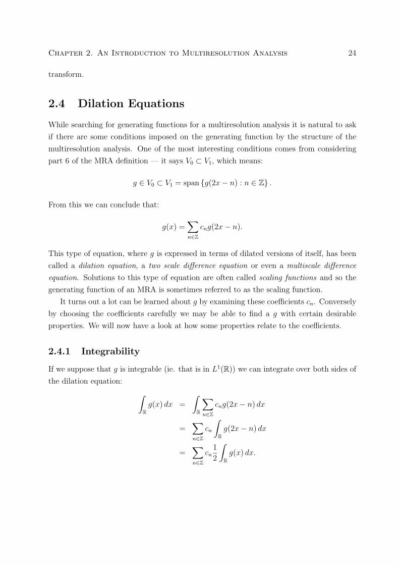
2.6.1 Haar Wavelets
In the Haar case we took g(x) = χ[0,1)(x), and we worked out that g(2x) = χ[0, 12
). In this
case it is reasonably clear that:
g(x) = χ[0,1)(x) = χ[0, 12
)(x) + χ[ 12,1)(x) = g(2x) + g(2x− 1).
So writing this in the form:
g(x) =∑n∈Z
cng(2x− n)
We get c0 = 1, c1 = 1 and all the other cn = 0. So using the formula we get:
w(x) =∑k∈Z
(−1)kc1−kg(2x− k) = g(2x)− g(2x− 1).
A picture of this Haar wavelet is shown in Figure 2.6.
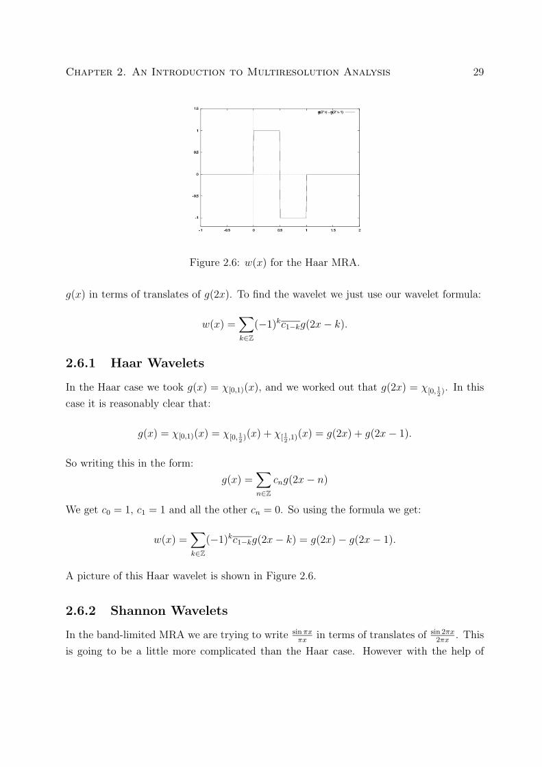
2.6.2 Shannon Wavelets
In the band-limited MRA we are trying to write sinπxπx
in terms of translates of sin 2πx2πx
. This
is going to be a little more complicated than the Haar case. However with the help of
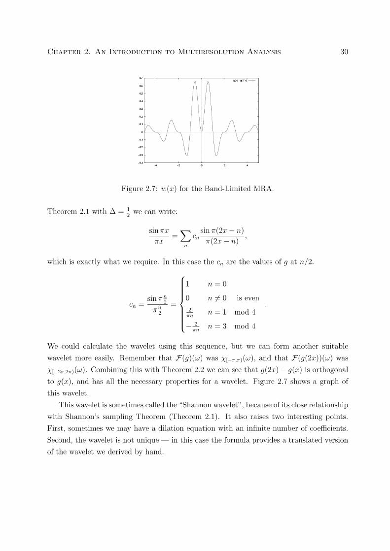
Chapter 2. An Introduction to Multiresolution Analysis 30
Figure 2.7: w(x) for the Band-Limited MRA.
Theorem 2.1 with ∆ = 12
we can write:
sin πx
πx=∑n
cnsin π(2x− n)
π(2x− n),
which is exactly what we require. In this case the cn are the values of g at n/2.
cn =sin π n
2
π n2
=
1 n = 0
0 n 6= 0 is even
2πn
n = 1 mod 4
− 2πn
n = 3 mod 4
.
We could calculate the wavelet using this sequence, but we can form another suitable
wavelet more easily. Remember that F(g)(ω) was χ[−π,π)(ω), and that F(g(2x))(ω) was
χ[−2π,2π)(ω). Combining this with Theorem 2.2 we can see that g(2x)− g(x) is orthogonal
to g(x), and has all the necessary properties for a wavelet. Figure 2.7 shows a graph of
this wavelet.
This wavelet is sometimes called the “Shannon wavelet”, because of its close relationship
with Shannon’s sampling Theorem (Theorem 2.1). It also raises two interesting points.
First, sometimes we may have a dilation equation with an infinite number of coefficients.
Second, the wavelet is not unique — in this case the formula provides a translated version
of the wavelet we derived by hand.
Chapter 2. An Introduction to Multiresolution Analysis 31
Figure 2.8: w(x) for one of Daubechies MRA’s.
2.6.3 Daubechies’ Wavelets
As commented earlier: Daubechies generating function was calculated so the coefficients
of its dilation equation satisfy all of the following equations.
1. c0 + c1 + c2 + c3 = 2,
2. c0c2 + c1c3 = 0,
3. c0 − c1 + c2 − c3 = 0,
4. 0c0 − 1c1 + 2c2 − 3c4 = 0.
The values which solve these equations are c0 = 14(1+√
3), c1 = 14(3+√
3), c2 = 14(3−√
3),
c3 = 14(1−
√3). Using these coefficients and g we can calculate w (Figure 2.8). In [3] she
includes a table of cn for progressively smoother generating functions (and so wavelets).
However the smoother the wavelet the wider its support.
2.7 How to draw these beasties
Until now we have carefully tiptoed around the question of how to draw Daubechies’
generating function. The problem is that we are presented with the coefficients for a
dilation equation, and left to find the solution ourselves.
Here we will examine an algorithm for drawing solutions to these equations. It makes
some rather bold assumptions, but these are justified in the literature [4].

Chapter 2. An Introduction to Multiresolution Analysis 32
We begin with a set of coefficients c0, . . . cN , whose sum is 2. We are attempting to
sketch a solution g to the dilation equation:
g(x) =N∑n=0
cng(2x− n).
We will assume that g(x) is zero outside [0, N ]. Now we examine the value of g at each of
the integers 0, 1, . . . , N using the dilation equation. We arrive at the following relations.
g(0) = c0g(0)
g(1) = c2g(0) + c1g(1) + c0g(2)
g(2) = c4g(0) + c3g(1) + c2g(2) + c1g(3) + c0g(4)
g(3) = c6g(0) + c5g(1) + c4g(2) + c3g(3) + c2g(1) + . . ....
g(N − 1) = cNg(N − 2) + cN−1g(N − 1) + cN−2g(N)
g(N) = cNg(N)
This is just an equation of the form:
~g = M~g,
where ~g = (g(0), g(1), . . . , g(N)) and M is a matrix with the cn and zeros as entries.
This, however, is just an eigenvector problem, which can be solved either by hand, or
by any of a host of computer programs. This provides us with the vector ~g and so the
value of g at the integers.
Now that we have found the values at the integers, we can find the values of g at m/2
for m ∈ Z using the dilation equation:
g(m
2
)=
N∑n=0
cng(m− n),
as m − n is an integer. Once we have g at half integers we can get g at quarter integers,
eighthes of integers and so on. To draw the graph we just join the dots!
Figure 2.9 contains a piece of C code which shows how simple this scheme is, for the
example of Daubechies generating function. The vector ~g was calculated and found to

Chapter 2. An Introduction to Multiresolution Analysis 33
#define STEP 0.0002
double c[] = 0.68301, 1.18301, 0.31699 , −0.18301;
double g(double x)
double tot;
int i;
if( x < 0.0 || x > 3.0 ) return 0.0;
if( fabs(x−0.0) < STEP/2 ) return 0.0;
if( fabs(x−1.0) < STEP/2 ) return 0.96593;
if( fabs(x−2.0) < STEP/2 ) return −0.25882;
if( fabs(x−3.0) < STEP/2 ) return 0.0;
tot = 0.0;
for( i = 0 ; i < 4 ; i++ ) tot += c[i] ∗ g(2.0 ∗ x − i);
return tot;
Figure 2.9: C code for estimating g
be (0.0, 0.96593,−0.25882, 0.0). This piece of code was used to produce Figure 2.5 and
indirectly Figure 2.8.
2.8 Conclusion
We have only scratched the surface of the huge body of material recently produced about
the discrete wavelet transform. The same goes for the two auxiliary subjects of multires-
olution analysis and dilation equations. A feeling for the volume and variety of work can
be got from [6].
Through the examples we have got some idea of the shapes that a multiresolution
Chapter 2. An Introduction to Multiresolution Analysis 34
analysis can come in, and saw that Fourier analysis does seem to have some link to mul-
tiresolution analysis. We will see more of this relationship in the following chapters.
One aspect of multiresolution analysis we did not touch on is what Meyer calls the
regularity of the MRA. This is a condition on the decay of g and its derivatives. [12]
provides great detail on not just this topic, but all of the theory mentioned here.
People have tried to extend wavelet and MRA theory into areas where Fourier analysis
has already been used. As long as we stay near Rn things are very successful: wavelets
have provided bases for whole hosts of spaces. Moving to other groups seems to have been
more troublesome. In [11] a definition of a multiresolution analysis on a locally compact
Abelian group is given, and wavelets are constructed on the Cantor dyadic group — but
this sort of work seems to be in the minority.
We have not said much about applications. It has been hinted that discrete wavelets and
multiresolution analysis are of use in audio and video signal processing. This is where much
of the excitement about wavelets is being generated. Wavelets have been used for both
video and audio compression in situations ranging from compressing the FBI’s fingerprint
collection to transmitting new generation TV signals.
Wavelets have also been put to statistical use for cleaning up data [20], and there is a
fast wavelet transform which is even faster than the fast Fourier transform. Some of these
many applications can be read about in Appendix 1 and 2 of [18], or in [17], [9] and [6].
Finally, we have said only a little about solving dilation equations. Much of what is
known is laid out in [4] and deals with only L1(Rn) solutions. In this case the solution
is usually unique. An application of dilation equations themselves is proposed in [1].
They examine a signal compression scheme in which the coefficients of a dilation equation,
which the signal satisfies, are transmitted in place of the signal. Unfortunately they make
incorrect assumptions about the uniqueness of L2(R) solutions, but the idea still stands.
Chapter 3
A New Construction for the Fourier
Transform
3.1 Introduction
Often complicated functions are not defined explicitly, but are rather defined in terms of
properties which we know they have. A common example might be the determinant of a
matrix. It can be defined either in terms of how to calculate it, or by properties such as
what happens when we multiply a row by a constant, or add two rows together. In fact, a
determinant can be defined by:
1. det : Rn×n → R
2. det(λ1~a1, λ2~a2, . . . , λn~an) = (λ1λ2 . . . λn) det(~a1,~a2, . . . ,~an)
where λi ∈ R and ~ai ∈ Rn for i = 1 . . . n.
3. det(. . . ,~ai, . . . ,~aj, . . .) = det(. . . ,~ai + ~aj, . . . ,~aj, . . .)
4. det(~e1, ~e2, . . . , ~en) = 1 where ~ejj=1..n is the usual basis for Rn.
What we will do is give an example of how this may be done for the Fourier transform
of functions in L2(R). The structure on which the determinant is built is the vector space.
The framework which we will use for building the Fourier transform is the multiresolution
analysis of L2(R) we introduced in Chapter 2. In this case we’re going to take the χ[0,1) as
g and consequently will end up working with the Haar MRA (Section 2.3.1).
35

Chapter 3. A New Construction for the Fourier Transform 36
The idea for this type of construction came from Chapter 2 of [12], where Meyer often
calculates the Fourier transform of a function from its multiresolution expansion. What
we do here is show that this calculation may actually be recast as a construction.
There is often debate about factors of√
2π when defining Fourier transforms, so to
begin with the Fourier transform for which we will give a new construction will be the
same as that given by:
F(f)(ω) =
∫ ∞−∞
e−iωxf(x) dx.
(This is the same as that used in Chapter 2.)
This means that the corresponding inverse transform will have a factor of 1/2π outside
the integral. While we have this formula is in front of us we will do one calculation: the
traditional Fourier transform of χ[0,1)
F(χ[0,1))(ω) =
∫ ∞−∞
e−iωxχ[0,1) dx =
∫ 1
0
e−iωx dx =1− e−iω
iω
3.2 Defining F on our MRA
First we define F on D =+∞⋃j=−∞
Vj, (with the Vj generated by taking g as χ[0,1)) in the
following way:
1. F : D → L2(R) is linear,
2. F(f tn)(ω) = eiωnF(f)(ω) where tn(x) = x+ n,
3. F(f dλ)(ω) = 1|λ|F(f)(ω
λ) where dλ(x) = λx and λ = 2n, n ∈ Z,
4. F(χ[0,1))(ω) = 1−e−iωiω
.
The linearity, translation and dilation rules are all basic properties of the Fourier trans-
form. The final rule pins down the Fourier transform, hopefully in a way we can extend
to all of L2(R). (We should really check that the translation rule and dilation rule are
consistent, that is: F(f tn tm) = F(f tn+m), F(f dλ dµ) = F(f dλµ) and
F(f tm dλ) = F(f dλ tmλ
).)
Theorem 3.1. Defining F using the above rules leads to a well defined function D →L2(R).
Chapter 3. A New Construction for the Fourier Transform 37
Proof. The rules clearly fix F on all ofD, in fact we can provide a formula. If f ∈ D =⋃Vj,
then we can write f as the finite sum:
f(x) =N∑
k=−N
akχ[0,1)(2Jx− k),
where f ∈ VJ . We can then apply our rules.
F(f)(ω) =N∑
k=−N
akF(χ[0,1) t−k d2J )(ω)
=N∑
k=−N
ak1
2JF(χ[0,1) t−k)(
ω
2J)
=N∑
k=−N
ake−ik
ω
2J
2JF(χ[0,1))(
ω
2J)
=N∑
k=−N
ake−ik
ω
2J
2J1− e−i
ω
2J
i ω2J
=1− e−i
ω
2J
iω
N∑k=−N
ake−ik ω
2J .
We are, however, left with some questions.
• Is 1−e−iωiω
in L2(R)? Once we know this we know that F(D) ⊂ L2(R) as L2(R) is
closed under translation, dilation, scaling, addition and multiplication by bounded
functions.
• Is F well defined? Some functions may have more than one expansion as sums
of translations and dilations of our basic function χ[0,1)(x). For example χ[0,1) =
χ[0, 12
) + χ[ 12,1).
• Does F actually satisfy parts 2 and 3 of its definition on all of D? It is reasonably
obvious that F is linear.
These points are dealt with in the following lemmas.
Lemma 3.2. ∥∥∥∥1− e−iω
iω
∥∥∥∥2
2
= 2π

Chapter 3. A New Construction for the Fourier Transform 38
Proof. For Theorem 3.1 all we need to show is that the L2 norm of 1−e−iωiω
is finite, but we
can do the calculation exactly using a mixture of brute force and contour integration:
∥∥∥∥1− e−iω
iω
∥∥∥∥2
2
=
∫ ∞−∞
∣∣∣∣1− e−iωiω
∣∣∣∣2 dω=
∫ ∞−∞
(1− e−iω)(1− eiω)
ω2dω
=
∫ ∞−∞
1− e−iω − eiω + 1
ω2dω
=
∫ ∞−∞
2(1− cosω)
ω2dω
= Re
(∫ ∞−∞
2(1− eiω)
ω2dω
)We can now integrate this on a contour which goes to infinity in the upper half plane,
and goes around zero on the lower: --The total for this is (2πi)(−2i) = 4π. The
contribution of the bit in the upper half plane goes to zero, and the bit around zero
contributes 2π as the contour is brought in, so the contribution along the real axis must
be 2π. So the total contribution is 2π as required.
Lemma 3.3. F as defined by the above rule is well defined.
Proof. First we verify this for the example: χ[0,1) = χ[0, 12
) + χ[ 12,1).
χ[0,1)(x) = χ[0, 12
)(x) + χ[ 12,1)(x)
= χ[0,1)(2x) + χ[1,2)(2x)
= χ[0,1)(2x) + χ[0,1)(2x− 1)
= χ[0,1) d2(x) + χ[0,1) t−1 d2(x)
We already know that: F(χ[0,1))(ω) = 1−e−iωiω
, so we now need to work out the Fourier
transform of the other two terms:
Chapter 3. A New Construction for the Fourier Transform 39
F(χ[0,1) d2)(ω) =1
2F(χ[0,1))
(ω2
)=
1
2
1− e−iω2iω
2
=1− e−iω2
iω;
F(χ[0,1) t−1 d2)(ω) =1
2F(χ[0,1) t−1)
(ω2
)=
1
2e−i
ω2F(χ[0,1))
(ω2
)=
1
2e−i
ω2
1− e−iω2iω
2
=e−i
ω2 − e−iω
iω.
So we get the required identity as follows:
F(χ[0, 12
) + χ[ 12,1))(ω) =
1− e−iω2iω
+e−i
ω2 − e−iω
iω=
1− e−iω
iω= F(χ[0,1))(ω)
Now showing that F is well defined is much easier, as using this we can break and join
adjacent steps. Indeed suppose f ∈ D, then as the Vj are increasing there is a smallest∗ j
for which f ∈ Vj. Then any expansion of f must have the same Fourier transform as the
one given by steps of size 2−j, by joining smaller steps.
Lemma 3.4. F has the following desired properties on all of D:
F(f tn)(ω) = eiωnF(f)(ω) for n ∈ Z,
F(f d2n)(ω) =1
2nF(f)(
ω
2n) for n ∈ Z.
Proof. We simply resort to writing:
f(x) =N∑
k=−N
akχ[0,1)(2Jx− k),
∗If f ∈ Vj∀j then f = 0, which can be checked easily by hand.
Chapter 3. A New Construction for the Fourier Transform 40
and then using:
F(f)(ω) =1− e−i
ω
2J
iω
N∑k=−N
ake−ik ω
2J .
As they say “simple algebraic manipulation yields”:
f tn(x) = f(x+ n)
=N∑
k=−N
akχ[0,1)(2J(x+ n)− k)
=N∑
l=−N
al+n2Jχ[0,1)(2Jx− l)
⇒ F(f tn)(ω) =1− e−i
ω
2J
iω
N∑l=−N
al+n2Je−il ω
2J
=1− e−i
ω
2J
iω
N∑k=−N
ake−i(k−n2J ) ω
2J
= einω1− e−i
ω
2J
iω
N∑k=−N
ake−ik ω
2J
= einωF(f)(ω),
and:
f d2n(x) = f(2nx)
=N∑
k=−N
akχ[0,1)(2J(2nx)− k)
=N∑
k=−N
akχ[0,1)(2J+nx− k)
⇒ F(f d2n)(ω) =1− e−i
ω
2J+n
iω
N∑k=−N
ake−ik ω
2J+n
=1
2nF(f)(
ω
2n).
So now we are at the stage where we have used our rules to define a linear transform
F : D → L2(R). We have shown that is it well defined, now it would be nice to extend it
Chapter 3. A New Construction for the Fourier Transform 41
to all of L2(R).
3.3 Extending F to L2(R)
We know that D ⊂ L2(R), and that D = L2(R). We wish to show that F : D → L2(R)
can be extended, by taking limits to F : L2(R)→ L2(R). That is: since for all f ∈ L2(R)
we may choose a sequence fn in D so that fn → f in L2(R), we could then define F(f) as
limF(fn).
If we can show that F : D → L2(R) is continuous then we can use the following lemma.
Lemma 3.5. Let N and S be Banach spaces. Let M be a dense subset of N . If we have
a continuous linear function φ : M → S, then we can extend φ to a function f on N by
taking limits, so that f is continuous and linear.
So extending F from D to all of L2(R) comes down to showing that F : D → L2(R) is
continuous with the L2 norm on the domain and range.
Lemma 3.6. F : D → L2(R) is continuous with the L2(R) norm on D. In fact:
‖F(f)‖2 =√
2π‖f‖2
Proof. Since F is linear showing it is bounded, is equivalent to showing it is continuous.
Take any f ∈ D, we must show:
‖F(f)‖ ≤ C‖f‖
where C doesn’t depend on f . Using our formulation from Theorem 3.1:
f(x) =N∑
k=−N
akχ[0,1)(2Jx− k).
Clearly this gives us ‖f‖22 =
∑Nk=−N |ak|2/2J . Then using the same calculation as in
Theorem 3.1 we find F(f) to be:
1− e−iω
2J
iω
N∑k=−N
ake−ik ω
2J .
We complete the calculation of ‖F(f)‖22 by brute force, contour integration and Lemma 3.2.

Chapter 3. A New Construction for the Fourier Transform 42
‖F(f)‖22
=
∫ ∞−∞
∣∣∣∣∣1− e−iω
2J
iω
∣∣∣∣∣2( N∑
k=−N
ake−ik ω
2J
)(N∑
l=−N
aleil ω
2J
)dω
=
∫ ∞−∞
2(1− cos ω2J
)
ω2
[(N∑
k=−N
|ak|2)
+
(∑k 6=l
akale−i(k−l) ω
2J
)]dω
=2π
2J
N∑k=−N
|ak|2 +∑k 6=l
akal
∫ ∞−∞
2(1− cos ω2J
)
ω2e−i(k−l)
ω
2J dω.
We want the integral on the right to be zero. By a change of variable, we reduce the
problem to showing that: ∫ ∞−∞
2(1− cosω)
ω2eirω dω = 0,
when r ∈ Z, r 6= 0. The imaginary part has to be zero, as 2(1−cosω)ω2 is even and sin rω is
odd. So now we’re down to:
∫ ∞−∞
2(1− cosω)
ω2cos rω dω
=
∫ ∞−∞
2 cos rω − 2 cosω cos rω
ω2dω
=
∫ ∞−∞
2 cos rω − cos((r + 1)ω)− cos((r − 1)ω)
ω2dω
= Re
(∫ ∞−∞
2eirω − ei(r+1)ω − ei(r−1)ω
ω2dω
).
Now, it’s easy to check that 2eirω − ei(r+1)ω − ei(r−1)ω has a double zero at ω = 0, and
so the integrand is analytic at zero. If r ≤ −1 or r ≥ 1 then we can integrate around a
loop in the lower or upper half plane respectively, so that the contribution for this part
of the loop goes to zero. But as the function is analytic everywhere, the integral around
the whole loop must be zero, and contribution from integrating along the real line must
be zero.
This means that as ‖f‖22 =
∑Nk=−N |ak|2/2J we simply get ‖F(f)‖2
2 = 2π‖f‖22. So we
see F is bounded with norm√
2π.

Chapter 3. A New Construction for the Fourier Transform 43
Now we can extend F as was desired, by combining the previous results.
Theorem 3.7. F : D → L2(R) can be extended continuously to F : L2(R) → L2(R) in a
unique way. Also this extension satisfies ‖F(f)‖2 =√
2π‖f‖2 for f ∈ L2(R).
Proof. Use Lemma 3.6 to show F is bounded and then use Lemma 3.5 extend F . The fact
that the norm is just scaled comes from Lemma 3.6, and the fact D is dense in L2(R).
We only needed ‖F(f)‖22 ≤ 2π‖f‖2
2 and so this stronger result is really just Plancherel’s
Theorem.
Corollary 3.8 (Plancherel’s Theorem). For f, g ∈ L2(R):
(f, g) = 2π(F(f),F(g))
where (·, ·) is the usual inner product on L2(R).
Proof. The fact that the norm is just scaled means we can apply the polarisation identity,
in the usual way, to show that the inner product is preserved in this Hilbert space.
3.4 Back to the traditional
We are now in a position to get the traditional Fourier transform, from our new definition.
This is a rather useful thing, as it allows us to check that no gremlins have crept in and
made our new transform different to the old.
Theorem 3.9. If f ∈ L2(R) and ∫ ∞−∞
f(x)e−iωx dx
converges for almost every value of ω then it agrees with F(f) almost everywhere.
Proof. We’ll do this in 3 stages, first for functions in D, then for compactly supported
functions in L2(R), and finally for the general case in the statement.
For f ∈ D: Suppose f ∈ VJ is supported on [−R,R]. Then we can write f(x) as:
f(x) =R2J−1∑k=−R2J
akχ[0,1)(2Jx− k)
Chapter 3. A New Construction for the Fourier Transform 44
Now f ∈ Vj,∀j ≥ J , so by noting that the coefficient of χ[0,1)(2jx − k) will just be
f( k2j
), we may also write f as:
f(x) =R2j−1∑k=−R2j
f(k
2j)χ[0,1)(2
jx− k)
We take the Fourier transform of this, which we can write out using the calculation
in Theorem 3.1.
F(f)(ω) =1− e−i
ω
2j
iω
R2j−1∑k=−R2j
f(k
2j)e−ik
ω
2j
=
(1− e−i
ω
2j
i ω2j
) 1
2j
R2j−1∑k=−R2j
f(k
2j)e−ik
ω
2j
Fixing ω we look at what happens as j →∞. The first term goes to 1. Remembering
that f is a step function, and so Riemann integrable, the second term becomes a
Riemann sum, leaving us with:
F(f)(ω) =
∫ R
−Rf(x)e−iωx dx.
For g ∈ L2(R) with compact support: From here it is easy to extend this to g ∈ L2(R)
with g supported on [−R,R]. First note that if we define
FR(f) =
∫ R
−Rf(x)e−iωx dx,
then FR(·)(ω) is continuous on L2(R), because:
FR(f)(ω) = (f(x), eixwχ[−R,R))
⇒ |FR(f)(ω)| ≤ ‖f‖2
∥∥eixwχ[−R,R)
∥∥2
= ‖f‖2
√2R.
This means if a sequence of functions gn converges in L2(R) then the sequence of
functions FR(gn) has a pointwise limit.
We can choose gn ∈ D supported on [−R,R] so that gn → g in L2(R) as n→∞ and
Chapter 3. A New Construction for the Fourier Transform 45
we now know that FR(gn) has a pointwise limit. Looking in L2(R):
limn→∞
FR(gn) = limn→∞
F(gn) = F(g),
where all the limits are in L2(R). Lemma 3.10 tells us that the pointwise limit must
agree with F(g) almost everywhere. That is:∫ R
−Rg(x)e−iωx dx = F(g)(ω) a.e. ω
So this Fourier transform agrees with the traditional one on functions in L2(R) with
compact support. As g is supported on [−R,R] we can just write this as:
F(g)(ω) =
∫ ∞−∞
g(x)e−iωx dx a.e. ω ∈ R.
What if the formula looks OK? If f is any function in L2(R) then the simple sequence
fn = fχ[−n,n) converges to f . What we would like to do is apply the formula to these
to get an indication of the Fourier transform of f . This leads us in the direction of
the improper integral we want.
F(fn)(ω) =
∫ ∞−∞
fn(x)e−iωx dx a.e. ω
=
∫ ∞−∞
χ[−n,n)(x)f(x)e−iωx dx
=
∫ n
−nf(x)e−iωx dx
We want to take a limit of this as n → ∞. If we keep away from the points where
this isn’t true for some n (which is a countable union of sets of zero measure, and so
of zero measure), then we get:
limn→∞
F(fn)(ω) =
∫ ∞−∞
f(x)e−iωx dx a.e. ω
The integral on the right is an improper integral, but that isn’t the problem. This is
a pointwise limit, and we need an L2(R) limit.
All is not lost however. We again use Lemma 3.10 as we have an L2(R) limit (the
Fourier transform) and a pointwise limit of the same sequence of functions and con-

Chapter 3. A New Construction for the Fourier Transform 46
clude these are be the same almost everywhere. That is: we know F(fn) → F(f)
in L2(R) and this means that if our improper integral converges to some function
almost everywhere, then it is the Fourier transform of f .
Lemma 3.10. Suppose fn → f in L2(R) and fn(x)→ g(x) pointwise for x ∈ R \N where
N has measure zero. Then f(x) = g(x) a.e. x ∈ R.
Proof. First note that ∀δ > 0, h ∈ L2(R):
‖h‖22 ≥
∫x:|h(x)|>δ
δ2 dx = δ2 |x : |h(x)| > δ| .
This means that:
|x : |fn(x)− f(x)| > δ| ≤ ‖fn − f‖22
δ2.
As fn → f in L2(R) we may choose an increasing sequence nj such that:∣∣∣∣x : |fn(x)− f(x)| > 1
2j
∣∣∣∣ ≤ 22j‖fn − f‖22 ≤
1
2j,
when n > nj, by making ‖fn − f‖22 ≤ 2−3j. Set:
Mj =⋃k>j
x : |fnk(x)− f(x)| > 1
2k
,
then |Mj| ≤ 12j
. Now off this set Mj we know that:
|fnk(x)− f(x)| ≤ 1
2k
if k > j. Thus fnk(x)→ f(x) pointwise off Mj, but remember that fnk(x) must also go to
g(x) off N , so we conclude f(x) = g(x) off Mj ∪N .
Finally let M = x : g(x) 6= f(x), then M ⊂ Mj ∪ N for all j ∈ N. Thus |M | ≤|Mj|+ |N | ≤ 1
2j+ 0 for all j ∈ N, so |M | = 0 as required.
Now we have the advantage that if we want to use a traditional proof we can, as we
have the integral formula for just about all the cases we could hope for!
Chapter 3. A New Construction for the Fourier Transform 47
3.5 Can we do better than that?
We defined the Fourier transform from the following 4 rules.
1. F : D → L2(R) is linear,
2. F(f tn)(ω) = eiωnF(f)(ω) where tn(x) = x+ n,
3. F(f dλ)(ω) = 1|λ|F(f)(ω
λ) where dλ(x) = λx and λ = 2n, n ∈ Z,
4. F(χ[0,1))(ω) = 1−e−iωiω
.
Surprisingly the fourth rule, which seems to kick start this definition of F , may be made
weaker. This is because we had to check that F was well defined in Lemma 3.3, which
may be turned around and made into deductions about what F(χ[0,1)) could possibly be.
Theorem 3.11. Using the first three rules above and the following:
• F(χ[0,1))(ω) is continuous at 0 and F(χ[0,1))(0) = 1
we may derive the fourth rule.
Proof. When we checked that F was well defined we made sure this rule was consistent
with χ[0,1) = χ[0, 12
) + χ[ 12,1). For this to be true we required:
F(χ[0,1))(ω) =1
2F(χ[0,1))
(ω2
)+
1
2e−i
ω2F(χ[0,1))
(ω2
)So letting f = F(χ[0,1)):
f(ω) =1
2
(1 + e−i
ω2
)f(ω
2)
=1
22
(1 + e−i
ω2
) (1 + e−i
ω22
)f(ω
22)
=
(1
2n
n∏k=1
(1 + e−i
ω
2k
))f(ω
2n)
=
(1
2n
2n∑r=1
e−iω2nr
)f(ω
2n)
=1
2ne−iω − 1
e−iω2n − 1
f(ω
2n).
Chapter 3. A New Construction for the Fourier Transform 48
Our new rule supposes f(ω) is continuous at zero, then (for fixed ω) we take the limit
of this expression as n→∞.
f(ω) =1− e−iω
iωf(0)
We also assumed that f(0) = 1, so:
F(χ[0,1))(ω) = f(ω) =1− e−iω
iω
So we have derived the old fourth rule as required.
This new rule could be motivated by the fact that χ[0,1) is an L1(R) function, and if we
are aiming for the traditional Fourier transform we want L1 functions to go to bounded
continuous functions.
We can’t do any better that this without changing the first 3 rules. Clearly we need
something to determine F up to constant multiples; something like F(χ[0,1))(0) = 1 or
‖F(χ[0,1))‖22 = 2π. If we also drop the continuity at 0 condition we leave open options such
as:
sign(ω)1− e−iω
iωwhere sign(x) =
+1 x > 0
0 x = 0
−1 x < 0
for F(χ[0,1)). It is easy to see that this will be consistent with the first 3 properties, because
they do not relate F(χ[0,1)) at negative ω with values at positive ω.
If we change the third rule to allow all λ 6= 0, then we may stand a better chance, as it
will relate F(χ[0,1))(ω) for negative and irrational ω to F(χ[0,1)) on positive dyadic rational
ω. This is pursued further in Chapter 4.
3.6 Extending properties of F
In Section 3.2 we defined F to have certain properties on D which we checked in Lemma 3.4.
We said what effect translation and dilation had on F when we dilated by two or translated
by an integer. We will extend these properties in two ways. First we will allow transla-
tion and dilation by any real number (except dilation by 0). Second we will show these
properties hold on all on L2(R) and not just on D. We will also establish another related
property of the Fourier transform.

Chapter 3. A New Construction for the Fourier Transform 49
Using Theorem 3.9 we easily can extend our translation and dilation rules to all trans-
lations tα with α ∈ R and dilations dλ with λ ∈ R\0. This just involves a simple change
of variable in the integral formula.
In a similar manner we can also examine the effect of translation on the Fourier trans-
form of a function. If f ∈ D, then f has compact support, and so we know:
F(f)(ω) =
∫ ∞−∞
f(x)e−iωx dx
This lets us deduce that:
F(f)(ω + α) =
∫ ∞−∞
f(x)e−i(ω+α)x dx a.e. ω
=
∫ ∞−∞
f(x)e−iαxe−iωx dx a.e. ω
= F(f(x)e−iαx)(ω) a.e. ω
So F(f) tα = F(f(x)e−iαx) when f ∈ D.
To express all this clearly, we’ll define 3 operators. These are translation T, dilation
D and rotation R. Our reason for defining these operators is that the properties of Fcan be expressed in terms of how F commutes with them. This notation is clearer than
the “f tα” notation above, and as all these operators are continuous it makes it easy to
extend a property of F on D to a property of F on L2(R).
• For all α ∈ R we define Tα : L2(R) → L2(R) by (Tαf)(x) = f(x + α). This is a
continuous linear operator with norm 1 on L2(R).
• For all λ ∈ R \ 0 we define Dλ : L2(R) → L2(R) by (Dλf)(x) = f(λx). This is a
continuous linear operator with norm |λ|− 12 .
• For all α ∈ R we define Rα : L2(R) → L2(R) by (Rαf)(x) = eiαxf(x). This is also
continuous linear operator with norm 1.
Let us now rephrase F ’s properties in terms of these operators. For all f ∈ D, α ∈ Rand λ ∈ R \ 0:
1. FTαf = RαFf ,
2. FDλf = 1|λ|D 1
λFf ,
Chapter 3. A New Construction for the Fourier Transform 50
3. FRαf = T−αFf .
So all the properties can be given in terms of relations of the form FA = BF . This
gives us a simple way to extend all these properties to L2(R) in one fell swoop. Suppose f
is in L2(R), and A,B are bounded linear operators on L2(R), such that FA = BF on D.
We can just take fn ⊂ D so fn → f as fn →∞, giving:
FAf = FA limn→∞
fn = limn→∞
FAfn = limn→∞
BFfn = B limn→∞
Ffn = BFf
3.7 The inverse Fourier transform
In exactly the same manner as we did for F we may define another transform G. We want
this to be an inverse for the Fourier transform so this time we define it with the following
rules:
1. G : D → L2(R) is linear,
2. G(f tn)(ω) = e−iωnG(f)(ω) where tn(x) = x+ n,
3. G(f dλ)(ω) = 1|λ|G(f)(ω
λ) where dλ(x) = λx and λ = 2n, n ∈ Z,
4. G(χ[0,1))(ω) is continuous at 0 and G(χ[0,1))(0) = 12π
.
These are the translation and dilation properties we would expect the inverse of the Fourier
transform to have (compare to those on page 36). It is easily guessed that G is very similar
to F , but with norm 1√2π
on L2(R) and slightly different properties. We would hope that
this turns out to be the inverse of the Fourier transform.
As we did for F , we write the properties of this new extended transform in terms of
the operators Tα, Dλ and Rα. For all f ∈ D, α ∈ R and λ ∈ R \ 0:
1. GTαf = R−αGf ,
2. GDλf = 1|λ|D 1
λGf ,
3. GRαf = TαGf .
Compare these to the properties of F above — the dilation rule is the same, and the minus
sign has moved from the rotation rule to the translation rule.
Chapter 3. A New Construction for the Fourier Transform 51
Theorem 3.12. The Fourier transform F : L2(R) → L2(R) is invertible, with inverse Gdefined as above.
Proof. We do already know that F is injective from Lemma 3.6. However, rather than
show it is surjective by hand, it is easier to show that G is the inverse of F on L2(R).
We examine I = FG. From the fact that F and G are continuous we see that I is
a continuous linear operator in L2(R) with norm 1 (the fact F scales the norm by√
2π,
and G scales it by 1/√
2π, means that I preserves the norm). Examining the effect of
translation and dilation:
ITnf = FGTnf = FR−nGf = TnFGf = TnIf
IDλf = FGDλf =1
|λ|FD 1
λGf =
|λ||λ|DλFGf = DλIf
So both translation and dilation commute with I. This, combined with the fact that Ipreserves the norm, is a pretty strong indication that it may be the identity. If we can
show that our generating function χ[0,1) is sent to itself by I we know it is the identity.
By using the equivalent of Theorem 3.9 for G we try to calculate G(1−e−iωiω
). As an
L2(R) function 1−e−iωiω
must have an image under G, and if the integral below converges to
an L2(R) function, then this must be the image of 1−e−iωiω
.
∫ ∞−∞
1− e−iω
iωeiωx dω
=
∫ ∞−∞
eiωx − eiω(x−1)
iωdω
=
∫ ∞−∞
sinωx− sinω(x− 1)
ωdω
=
∫ ∞−∞
sinωx
ωdω −
∫ ∞−∞
sinω(x+ 1)
ωdω
= sign(x)
∫ ∞−∞
sinω
ωdω − sign(x− 1)
∫ ∞−∞
sinω
ωdω
= (sign(x)− sign(x− 1))π
= 2πχ[0,1) a.e. ω
When we put in the 12π
factor for G we get exactly what we wanted. Similarly we
can check I ′ = GF is also the identity and so we conclude that G = F−1 and so F is
Chapter 3. A New Construction for the Fourier Transform 52
invertible.
From now on we will use F−1 for G when talking about the inverse of the Fourier
transform on L2(R).
3.8 Higher dimensions
This definition works quite well in n dimensions too. There are really only two differences.
First the dilation equation becomes more complicated — instead of 2 terms we have 2n
terms. The second difference is that for each dimension we get a factor of
1− e−iω
iω
in the Fourier transform of the function generating the MRA. This is actually quite fortu-
nate, because it means all the integration we have to do splits into independent 1 dimen-
sional integrals.
We begin by defining the translation, dilation and rotation operators for Rn.
• For all ~α ∈ Rn we define T~α : L2(Rn) → L2(Rn) by (T~αf)(~x) = f(~x + ~α). This is a
continuous linear operator with norm 1 on L2(Rn).
• For all λ ∈ R \ 0 we define Dλ : L2(Rn)→ L2(Rn) by (Dλf)(~x) = f(λ~x). This is a
continuous linear operator with norm |λ|−n2 .
• For all ~α ∈ Rn we define R~α : L2(Rn) → L2(Rn) by (R~αf)(~x) = ei~α·~xf(~x). This is
also continuous linear operator with norm 1.
We now define the Fourier transform, more or less as before. Let Q be the unit cube
[0, 1)n, and Dn be all the functions in the MRA of L2(Rn) generated by χQ. Now let F be
defined by:
1. F : Dn → L2(Rn) is linear,
2. FT~n = R~nF where ~n ∈ Zn,
3. FDλ = 1|λ|nFD 1
λwhere λ = 2n, n ∈ Z,
4. F(χQ)(~ω) is continuous at ~0 and F(χQ)(~0) = 1.

Chapter 3. A New Construction for the Fourier Transform 53
Our first task will be to derive F(χQ)(~ω), as we did for the 1 dimensional case in
Theorem 3.11. The proof is basically the same, but involves some work with a more
complicated dilation equation.
Theorem 3.13. If F is defined by the above rules then:
F(χQ)(~ω) =n∏k=1
1− e−iωkiωk
where ~ω = (ω1, ω2, . . . , ωn).
Proof. Our proof of Theorem 3.11 involved looking at a dilation equation that χ[0,1) satis-
fied. We have to find the equivalent equation for χQ. Examining the 1, 2 and 3 dimensional
cases it becomes apparent that the equation we are looking for is:
χQ =∑
~r∈0,1nD2T~rχQ
That is: the unit cube is the union of the cubes of side 1/2, which have had their origins
translated to each of the corners of a cube of side 1/2 at the origin.
Now we take the transform of this and apply our dilation and translation rules to get:
F(χQ) =∑
~r∈0,1n
1
2nD 1
2R~rF(χQ)
Rewriting this with f for F(χQ) and looking at a point ~ω we find:
f(~ω) =1
2nf
(~ω
2
) ∑~r∈0,1n
e−i~r·~ω2
Concentrating on the sum for the moment, we pluck off each component of ~ω. If ~x =
(x1, x2, . . . xn) we denote (x2, . . . xn) by ~x′.∑~r∈0,1n
e−i~r·~ω2 =
∑~r∈0,1n−1
(e−i
0·ω12 + e−i
1·ω12
)e−i
~r·~ω′2
=(
1 + e−iω12
)(1 + e−i
ω22
) ∑~r∈0,1n−2
e−i~r·~ω′′
2
=n∏k=1
(1 + e−i
ωk2
)
Chapter 3. A New Construction for the Fourier Transform 54
We can now substitute this expression back into our equation for f(~ω):
f(~ω) =1
2nf
(~ω
2
) n∏k=1
(1 + e−i
ωk2
)=
1
2nMf
(~ω
2M
) M∏m=1
n∏k=1
(1 + e−i
ωk2m
)repeating M times
=1
2nMf
(~ω
2M
) n∏k=1
M∏m=1
(1 + e−i
ωk2m
)=
1
2nMf
(~ω
2M
) n∏k=1
2M∑r=1
e−iωkwM
r
= f
(~ω
2M
) n∏k=1
1
2Me−iωk − 1
e−iωK2M − 1
Letting M →∞, and remembering we assumed f was continuous at zero,
f(~ω) = f(~0)n∏k=1
1− e−iωkiωk
Finally using f(~0) = 1 gives the required result.
The remainder of the work to show everything is well defined, continuous, extendible,
and invertible is the same as that for the one dimensional case, except for the fact that we
have multidimensional integrals, which split nicely into n one dimensional integrals. To
give the idea we will prove one of the results, the counterpart of Lemma 3.6.
Lemma 3.14. If f ∈ Dn then ‖f‖22 = C‖Ff‖2
2, where C = (2π)n.
Proof. Keeping a close eye on Lemma 3.6 we first write f in the form:
f(~x) =∑~r
a~rχQ(2J~x− ~r)
where the sum is over some finite subset of Zn and J ∈ N. As in Lemma 3.6 we note that
‖f‖22 =
∑|a~r|2/2Jn. Taking the Fourier transform we see:
F(f)(~ω) =
(n∏k=1
1− e−iωk2J
iωk
)∑~r
a~re−i~r·~ω
2j
Chapter 3. A New Construction for the Fourier Transform 55
Rearranging so that all the ωk terms are within the product:
F(f)(~ω) =∑~r
a~r
(n∏k=1
1− e−iωk2J
iωke−i
rkωk2j
)
Now we can work out the norm, by splitting the multiple integral, and using our original
calculation in Lemma 3.6:
‖Ff‖22
=
∫Rn
∑~r
a~r∑~s
a~s
n∏k=1
∣∣∣∣∣1− e−iωk2J
iωk
∣∣∣∣∣2
e−irkωk
2j eiskωk
2j d~ω
=∑~r
∑~s
a~ra~s
n∏k=1
∫R
∣∣∣∣∣1− e−iωk2J
iωk
∣∣∣∣∣2
e−irkωk
2j eiskωk
2j dωk
=∑~r
∑~s
a~ra~s
n∏k=1
2π
2Jδrksk
=∑~r
|a~r|2(
2π
2J
)n= (2π)n‖f‖2
2
as required.
3.9 Lp(Rn) for other p.
Extending F to L2(Rn) is only one direction in which we can expand — we can also make
extensions in other directions. The traditional definition of the Fourier transform provides
us with a definition for F on Lp(Rn) when 1 ≤ p ≤ 2. We can use our definition on all
these spaces too. In general F : Lp(Rn)→ Lq(Rn) with 1 ≤ p ≤ 2 and 1p
+ 1q
= 1. However
there are no inversion results, Plancherel’s Theorem or the like to look for when p 6= 2.
This means all we are left to do is prove that F is bounded from and to the correct spaces
(the equivalent of Lemma 3.6).
We have already dealt with the case p = 2, and first deal with the other extreme: the
case where p = 1. In this case F : L1(Rn)→ L∞(Rn), and we wish to show it is bounded.
For the sake of simplicity we will look at R instead of Rn.
Lemma 3.15. If we take our definition of F on D and examine F : D → L∞(R) we see
F is a bounded operator when D is given the norm it inherits as a subset of L1(R).

Chapter 3. A New Construction for the Fourier Transform 56
Proof. As in Lemma 3.6 we begin by writing f as:
f(x) =N∑
k=−N
akχ[0,1)(2Jx− k).
We note that ‖f‖1 =∑Nk=−N |ak|
2J. Again, exactly as in Lemma 3.6, we calculate the Fourier
transform:
(Ff)(ω) =1− e−i
ω
2J
iω
N∑k=−N
ake−ik ω
2J .
Estimating the L∞(R) norm of this is now a simple matter.
‖Ff‖∞ ≤ supω∈R
∣∣∣∣∣1− e−iω
2J
iω
N∑k=−N
ake−ik ω
2J
∣∣∣∣∣≤ sup
ω∈R
N∑k=−N
|ak|
∣∣∣∣∣1− e−iω
2J
iωe−ik
ω
2J
∣∣∣∣∣=
N∑k=−N
|ak| supω∈R
∣∣∣∣∣1− e−iω
2J
iω
∣∣∣∣∣=
N∑k=−N
|ak|1
2J
= ‖f‖1
The second last step may be verified by basic calculus and graph sketching (see Figure 3.1
for the idea).
So we can now extend F to all of L1(R), in the same was as we extended F from D to
L2(R) earlier.
Theorem 3.16. We may extend F : D → L∞(R) continuously to a bounded operator
F1 : L1(R)→ L∞(R) with norm 1 (again D is taken with ‖.‖1).
Proof. We can use Lemma 3.5 to extend F now that we have proved Lemma 3.15. Showing
that the norm is less than or equal to one also comes from Lemma 3.15. Showing it cannot
be less than 1 comes from looking at the Fourier transform of χ[0,1).
Note that we have called this new transform F1, because at the moment we do not know
how closely related to F it is. They must agree on D, because they are both extensions of
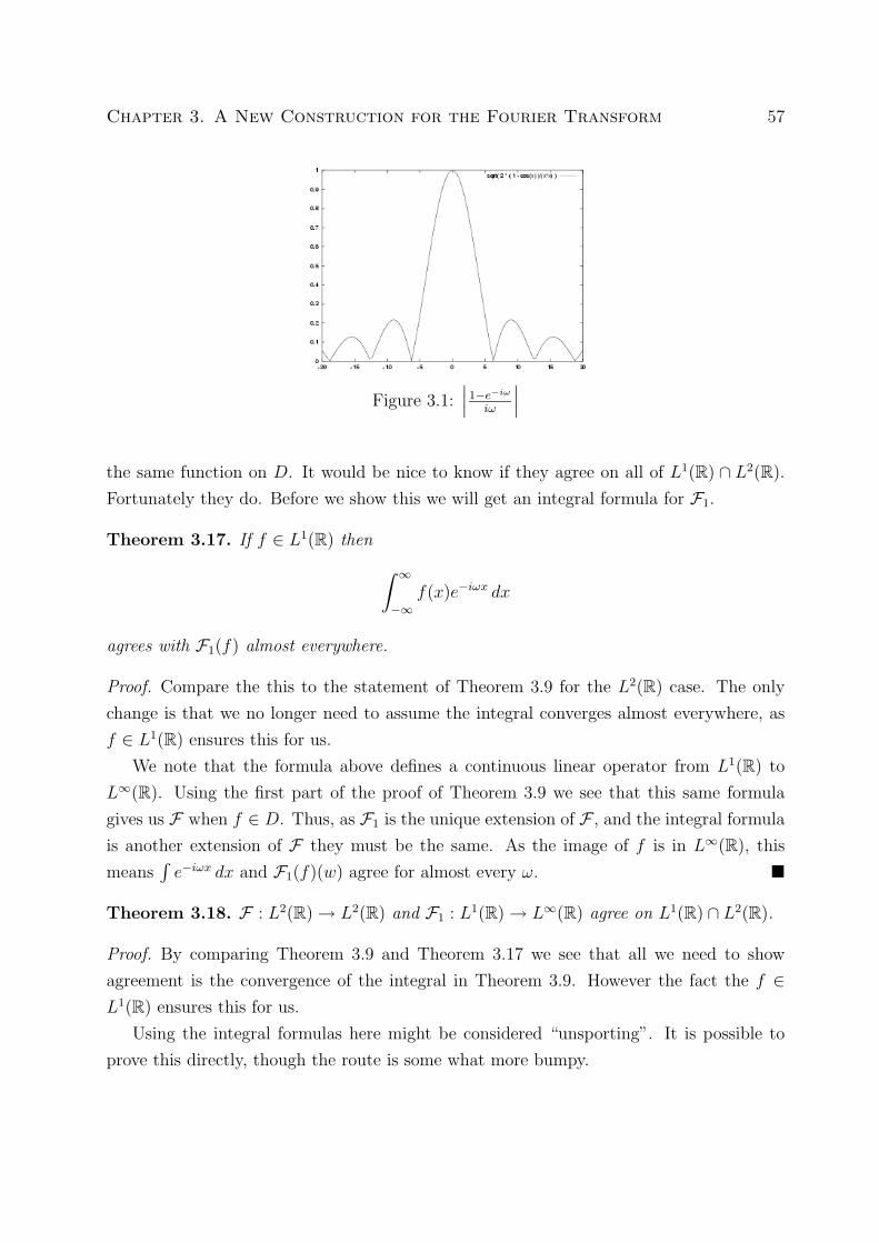
Chapter 3. A New Construction for the Fourier Transform 57
Figure 3.1:∣∣∣1−e−iωiω
∣∣∣the same function on D. It would be nice to know if they agree on all of L1(R) ∩ L2(R).
Fortunately they do. Before we show this we will get an integral formula for F1.
Theorem 3.17. If f ∈ L1(R) then ∫ ∞−∞
f(x)e−iωx dx
agrees with F1(f) almost everywhere.
Proof. Compare the this to the statement of Theorem 3.9 for the L2(R) case. The only
change is that we no longer need to assume the integral converges almost everywhere, as
f ∈ L1(R) ensures this for us.
We note that the formula above defines a continuous linear operator from L1(R) to
L∞(R). Using the first part of the proof of Theorem 3.9 we see that this same formula
gives us F when f ∈ D. Thus, as F1 is the unique extension of F , and the integral formula
is another extension of F they must be the same. As the image of f is in L∞(R), this
means∫e−iωx dx and F1(f)(w) agree for almost every ω.
Theorem 3.18. F : L2(R)→ L2(R) and F1 : L1(R)→ L∞(R) agree on L1(R) ∩ L2(R).
Proof. By comparing Theorem 3.9 and Theorem 3.17 we see that all we need to show
agreement is the convergence of the integral in Theorem 3.9. However the fact the f ∈L1(R) ensures this for us.
Using the integral formulas here might be considered “unsporting”. It is possible to
prove this directly, though the route is some what more bumpy.
Chapter 3. A New Construction for the Fourier Transform 58
1. If f ∈ L1(R) ∩ L2(R) has compact support then it is possible to choose fn in D so
that fn → f in L1(R) and fn → f in L2(R).
2. The definitions say Ff = limFfn in L2(R) , and F1f = limFfn in L∞(R).
3. Now we examine Ff and F1f in L2(R) and L∞(R) respectively. It can be shown
that these are the same almost everywhere.
4. Now we know F and F1 agree on compactly supported functions in L1(R) ∩ L2(R).
5. Now let g be any function in L1(R) ∩ L2(R). It is easy to show that gn = gχ[−n,n)
converges to g in both L1(R) and L2(R).
6. Again by the definitions Fg = limFgn in L2(R) and F1g = limF1gn in L∞(R).
7. Again we can show Fg = F1g because we now know Fgn = F1gn.
So, after some ado we have shown that we can define F on L1(R) and L2(R), and that
F agrees on the intersection. This is a large part of the hard work involved with defining
F on any Lp(R) (with 1 ≤ p ≤ 2) completed, due to the following lemma.
Lemma 3.19. Let f be in Lp(R) with 1 ≤ p ≤ 2. Then we can find f1 ∈ L1(R) and
f2 ∈ L2(R) so that f(x) = f1(x) + f2(x).
Proof. Define f1 as follows and set f2 = f − f1.
f1(x) =
f(x) |f(x)| ≥ 1
0 otherwise.
Then using p ≥ 1 and |y| ≥ 1 implies |y| ≤ |y|p we see that:
‖f1‖1 =
∫|f(x)|≥1
|f(x)| dx ≤∫
|f(x)|≥1
|f(x)|p dx ≤ ‖f‖pp,
so f1 ∈ L1(R). Similarly for f2 we note that p < 2 and |y| ≤ 1 implies |y|2 ≤ |y|p and so:
‖f2‖22 =
∫|f(x)|>1
|f(x)|2 dx ≤∫
|f(x)|>1
|f(x)|p dx ≤ ‖f‖pp, .
Chapter 3. A New Construction for the Fourier Transform 59
Thus f2 ∈ L2(R) as required.
Our final extension can now be performed in a straight forward manner.
Theorem 3.20. For each 1 ≤ p ≤ 2 we can extend F : D → (L2(R) ∩ L∞(R)) to
F : Lp(R)→ (L2(R) + L∞(R)) in a well defined manner.
Proof. For each f ∈ Lp(R) we write f = f1 + f2 where f1 ∈ L1(R) and f2 ∈ L2(R). Then
we define:
Ff = F1f1 + Ff2.
This definition is independent of the choice of f1 and f2, for suppose f = g1 + g2 with
g1 ∈ L1(R) and g2 ∈ L2(R) then:
f1 − g1 = f2 − g2.
So f1 − g1 is in both L1(R) and L2(R) so Theorem 3.18 tells us F1(f1 − g1) = F(f2 − g2).
Rearranging gives F1(f1) + F(f2) = F1(g1) + F(g2) as required.
We have not said if F defined in this manner is bounded, and what norm we should
use on the range. It seems that these calculations with the new construction are no easier
than with the original construction. For this reason it would seem acceptable to use some
general piece of operator interpolation theory which would tell us F : Lp(R)→ Lq(R) in a
bounded manner when 1p
+ 1q
= 1. Chapter 5 of [16] deals with this sort of interpolation in
detail.
3.10 Conclusions
This seems to be a new way of constructing the Fourier transform on L2(Rn). It is quite
straight forward, and doesn’t need many other complicated results (the main one might
be similar to Lusin’s theorem, which would be used to show the dyadic step functions are
dense in Lp(Rn)).
Traditional constructions of the Fourier transform (on L2(Rn)) usually begin with defin-
ing the Fourier transform on some dense subset, such as L2(Rn) ∩ L1(Rn) or the Schwartz
class S of C∞ functions which decay rapidly†. These spaces are chosen because the Fourier
†Rapidly here means that:
sup∣∣∣∣xα ∂|β|∂xβ
f(x)∣∣∣∣ <∞
Chapter 3. A New Construction for the Fourier Transform 60
transform will be well behaved there, for instance the integral formula is well defined on
L2(Rn)∩L1(Rn), and the Fourier transform is invertible on S and very well behaved there.
The approach we have used is similar in that we began by defining F on a dense subspace
— the dyadic step functions D.
The definition used on these subspaces is usually the integral formula. In our MRA
based construction we have used a set of desired properties to define Fourier transform, so
this is one place where this new construction differs.
Once the definition has been made, the extension to all of L2(Rn) is carried out in the
obvious way — by proving that the transform is bounded on the chosen dense subspace
and then extending it continuously. Here the MRA based method is, in spirit, the same
(we also extend F continuously) however the proof that F is bounded is quite different.
The usual demonstration that F is bounded uses the convolution result: F(f ∗ g) =
F(f)F(g) for the Fourier transform. This is applied to f and g(x) = f(−x) to get a h with
the property h = |f |2 and after some convergence, invertibility and continuity arguments
h(0) is examined to discover:∫|f |2 =
∫h = h(0) =
∫f(x)g(0− x) dx =
∫ff =
∫|f |2
The convergence issues surrounding this are usually tricky and involve some actual calcu-
lation of integrals. Even the slick treatment of this subject in Chapter 1 of [16] involves
some messy integration. In comparison the MRA method seems a relatively straight for-
ward piece of contour integration.
The other main result, the invertibility of F on L2(Rn), is usually obtained by noting
that it is invertible on the dense subspace and then extending continuously. Showing that
the transform is invertible on your dense subspace is not straight forward, but has usually
been dealt with on the way to showing that F is bounded. Here the MRA construction
involves a relatively simple piece of integration to show that a constructed operator is
actually the inverse of F .
The L1(Rn) case, in the MRA construction, is very similar to the case L2(Rn). Tradi-
tional constructions on L1(Rn) are more or less trivial, as the integral formula is as well
behaved as is needed on L1(Rn). The MRA construction does not seem to shed any light
on the Lp(R) case and so we resort to traditional techniques to form the Fourier transform
here.
for all non-negative n-tuples α, β.
Chapter 3. A New Construction for the Fourier Transform 61
There are disadvantages to the MRA based method — it doesn’t provide a nice link to
the Fourier transform of tempered distributions‡, as the dyadic step functions aren’t really
suitable as test functions. Neither does it easily provide access to the convolution results.
The reason no convolution result is easily forthcoming seems to be because the convolution
of two step functions is not a step function.
A possible way around these problems might be to use a different generating function.
Something like e−x2
might be quite suitable, first because it is a suitable test function
for distributions, and second because it is almost its own Fourier transform. The other
possible way around would be to use the integral formula, which we may as well use if the
proof using it is more straight forward.
In comparison the translation, dilation and rotation properties we used to define the
Fourier transform are easily derived from the integral formula, and so are not difficult to
obtain in any of the traditional constructions.
It should also be possible to use wavelets instead of MRA for the basis of these con-
structions. This would have advantages, as we should have fewer problems with checking
if things are well defined (this is as wavelets form a basis, and we will have uniqueness
of representation). On the other hand higher dimensional wavelets can be more irregular
than higher dimensional MRAs, so there could be a down side too.
A final note would be that it should be possible to do similar studies of other transforms
(Hilbert, Laplace?), and on other spaces (Heisenberg group?). I have looked at some
of these, but found that the integration is not as straight forward, and so reduces the
usefulness of the method. This, naturally, is not to say that such a study is impossible or
uninteresting.
‡The construction on S provides a strong link.
Chapter 4
A Uniqueness Result for the Fourier
Transform
4.1 Introduction
What we now aim to find out is: are dilation, translation and rotation conditions enough
to pin down the Fourier transform exactly? From the previous section it is apparent that
given rules about how a linear transform behaves when composed with translation and
dilation, we can make deductions about the image of functions satisfying certain dilation
equations.
If we consider a linear transform A : L2(R)→ L2(R) with:
ATnf = RnAf ∀n ∈ Z
ADλf =1
|λ|D 1
λAf ∀λ = 2n, n ∈ Z,
then by looking at the composition F−1A we would get an identity-like transform. More
specifically, the solution space of any dilation equation of the form:
f(x) =∑n
cnf(2x− n)
would be sent to itself under F−1A, because F−1 “undoes” the intertwining that A does.
For instance: we know χ[0,1) satisfies:
f(x) = f(2x) + f(2x− 1)
62

Chapter 4. A Uniqueness Result for the Fourier Transform 63
so F−1Aχ[0,1) also satisfies it. We can conclude that Aχ[0,1) = Ff , where f is a solution of
the above dilation equation. Now, if we know the image of some function (in this example
Aχ[0,1)) we could proceed as we did for F in Chapter 3 to try to determine this transform
on all of L2(R).
So looking for solutions of dilation equations, can be related to looking for transforms
A which have certain translation and dilation properties.
It would be more accurate to write the above dilation equations in the form:
f =∑n
cnD2Tnf
because we will be looking for L2(R) solutions, which may fail to satisfy the dilation
equation on some set of measure zero. We look for L2(R) solutions because we will want
the Fourier like transforms to be linear maps on L2(R).
We could look for solutions in other spaces of functions. The case where the Fourier
transform of the solution is continuous has been examined in some detail by those inter-
ested in wavelets. Here people are looking for compactly supported functions in Lp(R)
— Daubechies and Lagarias deal with L1(R) solutions of general dilation equations in [4].
When p ≥ 1 the compactly supported Lp(R) case is less general than the L1(R) case.
Others have dealt with this, for example [21].
4.2 A simple start
One beginning would be to solve dilation equations that hold everywhere. In looking for
solutions in L2(R) we will not have this option, but this search gives us a foothold.
We observe that by chopping χ[0,1) at α ∈ (0, 1) we get a two pieces χ[0,α) and χ[α,1) —
this means χ[0,1) satisfies the dilation equation:
χ[0,1)(x) = χ[0,1)
(xα
)+ χ[0,1)
(x− α1− α
)for any α ∈ (0, 1).
Theorem 4.1. Let g : R→ R be such that:
g(x) = g(xα
)+ g
(x− α1− α
)

Chapter 4. A Uniqueness Result for the Fourier Transform 64
∀α ∈ (0, 1). Then g is a constant multiple of χ[0,1) except at 0 and 1.
Proof. We prove this by varying the parameter α. Setting x = 0:
g(0) = g(0) + g
(−α
1− α
)0 = g
(−α
1− α
)As α ranges over (0, 1), −α
1−α ranges over (−∞, 0), thus g is supported on [0,∞). Setting
x = 1 leads to a similar cancelation giving:
0 = g
(1
α
)and as α ranges over (0, 1), 1/α goes from 1 to ∞. So now we know g is supported on
[0, 1]. Now to get the values in the middle we set x = 1/2:
g
(1
2
)= g
(1
2α
)+ g
(1− 2α
2(1− α)
)Now when α ∈ (0, 1
2), 1/2α > 1 and (1 − 2α)/2(1 − α) ranges over (0, 1
2). Similarly if
α ∈ (12, 1), (1 − 2α)/2(1 − α) < 0 and 1/2α ranges over (1
2, 1). Filling in to the above we
find that g(x) = g(1/2) for x ∈ (0, 1).
We also observe that by putting x = α = 1/2 gives that g(0) + g(1) = g(1/2).
Remark 4.1. It is worth noting that we have used a lot of dilation equations in the proof
of this theorem, one for each α ∈ (0, 1) — an uncountable number. This is the theorem’s
undoing in L2(R).
4.3 A useful counterexample
The unlikely looking function,
log
∣∣∣∣1− 1
x
∣∣∣∣ ,

Chapter 4. A Uniqueness Result for the Fourier Transform 65
Figure 4.1: φ(x)
is actually closely related to χ[0,1). It is the Hilbert transform∗ of χ[0,1), and so has Fourier
transform:
−i sign(ω)1− e−iω
iω.
While trying to weaken the definition of the Fourier transform in Section 3.5 we came
up with this type of function as a possible contender for the image of χ[0,1). To rule it out
we introduced the continuity at 0 clause. Another reason that this function is interesting
is because it only narrowly misses being in L1(R).
Lemma 4.2. Let φ(x) be given by:
φ(x) = log
∣∣∣∣1− 1
x
∣∣∣∣ .Then φ ∈ Lp(R) for 1 < p <∞.
Proof. A sketch of φ (Figure 4.1), shows we have two things to worry about. The tails of
the function, and the two points where it blows up. It does also show that the function is
symmetric (under reflection in (1/2, 0)), so at least we only have to do one tail and either
of the bad points.
∗The Hilbert transform H of a function f is usually given to be
(Hf)(x) =1π
∫f(t)x− t
dt.
This corresponds to multiplying the Fourier transform by −i sign(ω). The Hilbert transform is mentionedin most books dealing with the theory of Fourier transforms, for example [16].

Chapter 4. A Uniqueness Result for the Fourier Transform 66
The tails are easy to deal with. Looking at
dφ
dx=
1
x2 − x
we see that φ(x) behaves like − 1x
in the limit as |x| → ∞. To make this precise we compare
− 1x
with φ(x) on (2,∞). Since the limit of both is zero we can write (for a ≥ 2):
φ(a) +1
a=
∫ a
∞
d
dx
(φ(x) +
1
x
)dx
=
∫ a
∞
1
x2 − x− 1
x2dx
=
∫ a
∞
1
x2(x− 1)dx∣∣∣∣φ(a) +
1
a
∣∣∣∣ =
∫ ∞a
1
x2(x− 1)dx
≤∫ ∞a
1
(x− 1)3dx
=1
2(a− 1)2
If we look at this when x is large (say |x| > 2) we see the tails of 1a
and 12(a−1)2 are in Lp(R)
when p > 1, so the tails of φ are also in Lp(R).
Now we turn to the singularity at 0. We try to see how bad it is in the same way we
might examine a pole, by calculating:
limx→0
xnφ(x)
for n > 0. We will have to use L’Hopital’s rule here.
limx→0
log∣∣1− 1
x
∣∣x−n
= limx→0
1x2−x
−nx−(n+1)
= limx→0
xn+1
−n(x2 − x)
= limx→0
xn
−n(x− 1)= 0.
Chapter 4. A Uniqueness Result for the Fourier Transform 67
We may choose n so that np < 1, as p < ∞. So ∀ε > 0 ∃ δ > 0 so that when |x| < δ we
know: ∣∣∣∣xn log
∣∣∣∣1− 1
x
∣∣∣∣∣∣∣∣ < ε∣∣∣∣log
∣∣∣∣1− 1
x
∣∣∣∣∣∣∣∣ <ε
|x|n∫ δ
−δ
∣∣∣∣log
∣∣∣∣1− 1
x
∣∣∣∣∣∣∣∣p dx <
∫ δ
−δ
εp
|x|npdx
< ∞.
So now we know the tails and singularities contribute only a finite amount to the Lp(R)
norm, and the remaining bits are bounded and have compact support, so φ has finite Lp(R)
norm as required.
This example leads in to three useful pieces of information.
Remark 4.2. Examining its dilation properties we find φ satisfies all the criteria of Theo-
rem 4.1, except when φ is evaluated at 0 and 1. At x 6= 0, α, 1:
φ(xα
)+ φ
(x− α1− α
)= log
∣∣∣1− α
x
∣∣∣+ log
∣∣∣∣1− 1− αx− α
∣∣∣∣= log
∣∣∣∣(x− αx)(
x− α− 1 + α
x− α
)∣∣∣∣= log
∣∣∣∣1− 1
x
∣∣∣∣ = φ(x)
The fact that the set over which α ranges has non-zero measure causes a problem. When
we consider all the equations together, the set where at least one of the dilation equations
fails to hold is: ⋃α∈(0,1)
0, α, 1 = [0, 1],
which has non-zero measure. This is why we cannot try to use Theorem 4.1 when we want
solutions which hold almost everywhere.
Remark 4.3. The symmetries of φ are slightly different to those of χ[0,1). About the line
x = 1/2, φ is odd but χ[0,1) is even. Properties like odd and even can be expressed as

Chapter 4. A Uniqueness Result for the Fourier Transform 68
dilation type equations with negative scale factors. In this case:
χ[0,1)(x) = χ[0,1)(−x+ 1)
φ(x) = −φ(−x+ 1)
Remark 4.4. The fact that Fφ is Fχ[0,1) multiplied by some relatively uncomplicated
function is quite interesting. It will turn out to be profitable to look at the ratio of the
Fourier transforms of solutions to a given dilation equation.
4.4 How many solutions?
So we have found that χ[0,1) and φ both satisfy the simple dilation equation:
f(x) = f(2x) + f(2x− 1)
We might well suspect that the solution space of this equation is two dimensional, as it
has two terms, a dilation factor of two and its coefficients sum to two. If this were the case
all we would need to pin down the Fourier transform would be:
ATnf = RnAf ∀n ∈ Z
ADλf =1
|λ|D 1
λAf ∀λ = ±2n, n ∈ Z
because using the negative scales we could rule out φ by looking at the transformed versions
of the dilation equations in Remark 4.3.
Unfortunately, the solution space is not 2 dimensional, it is quite a lot bigger. To find
some more solutions we must go back to the way we found φ in the first place — by looking
at conditions on its transform.
Lemma 4.3. Let A : L2(R)→ L2(R) be a linear transform which satisfies:
ATnf = RnAf ∀n ∈ Z
ADλf =1
|λ|D 1
λAf ∀λ = ±2n, n ∈ Z
Chapter 4. A Uniqueness Result for the Fourier Transform 69
If we denote Aχ[0,1) by ψ, then ψ satisfies:
ψ(x) = e−ixψ(−x)
and:
ψ(x) =1
2
1− e−ix
1− e−ix2
ψ(x
2
)for almost all x ∈ R.
Proof. To get the first condition we rearrange the dilation equation:
χ[0,1)(x) = χ[0,1)(−x+ 1)
χ[0,1) = D−1T1χ[0,1)
Aχ[0,1) = AD−1T1χ[0,1)
= D−1AT1χ[0,1)
= D−1R1Aχ[0,1)
ψ(x) = D−1R1ψ(x) a.e. x ∈ R
ψ(x) = D−1eixψ(x) a.e. x ∈ R
ψ(x) = e−ixψ(−x) a.e. x ∈ R
To get the second we rearrange the dilation equation:
χ[0,1)(x) = χ[0,1)(2x) + χ[0,1)(2x− 1)
χ[0,1) = D2χ[0,1) +D2T−1χ[0,1)
Aχ[0,1) = AD2χ[0,1) +AD2T−1χ[0,1)
ψ =1
2D 1
2ψ +
1
2D 1
2AT−1χ[0,1)
ψ =1
2D 1
2ψ +
1
2D 1
2R−1ψ
ψ(x) =1
2ψ(x
2
)+
1
2e−i
x2ψ(x
2
)a.e. x ∈ R
ψ(x) =1
2
(1 + e−i
x2
)ψ(x
2
)a.e. x ∈ R
ψ(x) =1
2
1− e−ix
1− e−ix2ψ(x
2
)a.e. x ∈ R
Chapter 4. A Uniqueness Result for the Fourier Transform 70
Now to some extent we can see where we are going. Having a rule for dilation by 2n
tells us the relation between ψ(x) and ψ(2nx). Having a rule for dilation by −1 gives us a
relation between ψ(x) and ψ(−x).
It would even seem that these are the only constraints. We can use this to get some
results about solving general dilation equations. Indeed suppose that we have some solution
f0 to a dilation equation. When we take the Fourier† transform of this dilation equation
suppose we get:
f(x) = P (x)f(x
2
)Naturally we know f0 satisfies this. If we pick some function g so that g(x) = g(2x) for all
x ∈ R, then g(x)f0(x) will also satisfy this transformed dilation equation. If this g(x)f0(x)
is in L2(R) then we can take the inverse transform and we have a new solution to the
dilation equation.
This tells us that there are lots of solutions of our dilation equations. Daubechies and
Lagarias do write about this type of solution in [4], but the fact that they are looking for
f ∈ L1(R) means f is continuous. For this reason they reject these solutions in many cases
(the idea is that they only accept these solutions where either g is constant, or f0(x)→ 0
as x→ 0 and f0 and g are continuous).
They construct suitable g by choosing two period 1 functions g+ and g− and then define
g by:
g(x) =
g+ (log2 |x|) x > 0
g− (log2 |x|) x < 0
0 x = 0
.
The following lemma just makes a concrete case for our dilation equation:
f(x) = f(2x) + f(2x− 1).
Lemma 4.4. Let f0 = χ[0,1) and let E be a measurable subset of (1, 2). Define g on (1, 2)
so that g = χE, and extend g uniquely so that g(x) = g(−x) and g(x) = g(2x). Then:
f(x) = F−1 (gFf0) (x)
is a solution to f(x) = f(2x) + f(2x− 1).
†F would be a suitable A in Lemma 4.3

Chapter 4. A Uniqueness Result for the Fourier Transform 71
Proof. Since f0 is in L2(R), Ff0 ∈ L2(R). Let F =⋃n∈Z±2nE then:
∫R
|gFf0|2 dx =
∫F
|Ff0|2 dx
≤∫R
|Ff0|2 dx
< ∞
So gFf0 is in L2(R), so we can find F−1 of it.
Verifying it is a solution of the dilation equation is just a matter of working through
the algebra.
This more or less puts the last nail in the coffin of any attempt to try to uniquely
determine the Fourier transform using dilations by only powers of 2. Even with dilations
by negative factors we will still have a huge amount of freedom. Our only hope of success
is to introduce dilations by more scales.
4.5 Some more dilation equations
While proving Theorem 4.1 we used the fact that χ[0,1) was a solution of
f(x) = f(xα
)+ f
(x− α1− α
)for all α in (0, 1). Let’s see what happens if we have a transform A for which the dilation
property held for powers of both α and 1− α.
f = D 1αf + T−αD 1
1−αf
Note that we are going to need to use translation by many α now, and not just integers.
Af = AD 1αf +AT−αD 1
1−αf
Af = αDαAf +R−αAD 11−α
f
Af = αDαAf + (1− α)R−αD1−αAf
(Af)(x) = α(Af)(αx) + (1− α)e−iαx(Af)((1− α)x) a.e. x ∈ R

Chapter 4. A Uniqueness Result for the Fourier Transform 72
The first problem with this equation is that it is a three scale equation: 1, α and 1−α — this
means the equation can not easily be iterated. The equation that gave us the relationship
between x and 2x was a two scale equation, and this made it ideal for iteration. The second
problem is that we don’t have a good set to choose α from — if we take all the α ∈ (0, 1)
then we have a problem where we take the union of too many sets of measure 0, and end
up with a set of positive measure. We could try α ∈ Q∩ (0, 1) — but in Theorem 4.1 that
wouldn’t be good enough without an improved argument.
So we want a new set of dilation equations with the following properties:
• Each one should only contain 2 scales.
• There should be at most a countable number of them.
• They should be simple/regular enough that we can apply our translation and dilation
rules and see what happens.
Fortunately the next most obvious way of chopping up χ[0,1) provides us with exactly what
we need. All we do is chop χ[0,1) into n equal parts (n ∈ N).
χ[0,1)(x) = χ[0, 1n
)(x) + χ[ 1n, 2n
)(x) + · · ·+ χ[n−1n,1)(x)
= χ[0,1)(nx) + χ[0,1)(nx− 1) + · · ·+ χ[0,1)(nx− n+ 1)
Now we can prove a slightly more general version of Lemma 4.3.
Lemma 4.5. Suppose f satisfies:
f(x) =n−1∑r=0
f(nx− r)
for some n ∈ N and A is a linear transform with
ATmf = RmAf ∀m ∈ Z
ADλf =1
|λ|D 1
λAf ∀λ = ±nm, m ∈ Z
then Af denoted by f satisfies:
f(x) =1
n
1− e−ix
1− e−i xnf(xn
)
Chapter 4. A Uniqueness Result for the Fourier Transform 73
for almost all x ∈ R.
Proof. The proof is completely analogous to that of Lemma 4.3.
We can now see what effect having a rule for dilation by n has — it relates f(x) to
f(x/n). The next lemma shows that in Lp(R) the fact that this relation is true only almost
everywhere is not so important because we can redefine the function on a set of measure
zero so the relation between f(x) and f(x/n) is true everywhere.
Lemma 4.6. If f ∈ Lp(R) satisfies a finite non-zero dilation equation of scale α > 1, and
A : Lp(R) → Lq(R) has the dilation property for scale α and the translation property for
integers, then knowing f = Af on [αn, αn+1) determines f in Lq(R+).
Proof. We have supposed that f satisfies a dilation equation:
f =∑n
cnDαT−nf
Applying A and using the translation and dilation rules:
f =
(1
α
∑n
cne−ixn
α
)D 1
αf .
Or:
f(x) = P (x)f(xα
)a.e. x ∈ R.
P (x) is just a trigonometric polynomial and so is analytic, which means either P is iden-
tically 0 or P has a countable number of zeros. As the cn are not all zero P can not be 0,
so we conclude P (x) has a countable number of zeros.
If all things were well behaved we could iterate our relation to get (for n in N):
f( xαn
)=
f(x)n−1∏r=0
P(xαr
)f (xαn) =
n−1∏r=0
P (xαr) f(x).
Thus providing P (αnx) is nonzero and the original relation holds for αnx then given f(x)
we may find f(αnx)∀n ∈ Z. So if we know f on [αn, αn+1) and we want to know f at
Chapter 4. A Uniqueness Result for the Fourier Transform 74
x ∈ R+ we simply multiply x by some power of α until it lies in our interval [αn, αn+1) —
providing we avoid the bad points.
However, we can show that the set of these bad points is of measure zero. Let N be
the set of points where our original relation does not hold. Then the set of all bad points
is:
M =x ∈ R+ : P (αnx) = 0 or αnx ∈ N for some n ∈ Z
= αnx : P (x) = 0 and n ∈ Z ∪ αnx : x ∈ N and n ∈ Z
=⋃n∈Z
αnx : P (x) = 0 ∪⋃n∈Z
αnx : x ∈ N .
But this is the union of two countable unions of sets of measure zero, and so has measure
zero. Thus we can set f to be 0 on M without changing anything in Lq(R), and the relation
will then hold everywhere (as the relation will always hold if both f(x) and f(x/α) are
zero).
Remark 4.5. We should note that [0, ε] always contains an interval of the form [αn, αn+1)
for any ε > 0. This means knowing f on [0, ε] is enough to determine f on the whole
positive side.
Remark 4.6. We proved the lemma for α > 1, but the situation is essentially the same for
scales 0 < α < 1. Also, having a negative scale and related non-zero dilation equation lets
us determine f on R− from f on R+.
We can now see having a dilation rule and equation of scale n has more or less the same
effect as knowing one of scale 2. We know that allowing the scale to be 2 is not enough,
so for the moment let’s go to the other extreme and allow all n ∈ Z.
4.6 Pinning it down
We are now ready to present a way of pinning the Fourier transform down. To prove this
theorem we will need the following result:
Lemma 4.7. If g ∈ L1(R), and if
f(x) =
∫ x
−∞g(t) dt x ∈ (−∞,∞)
Chapter 4. A Uniqueness Result for the Fourier Transform 75
then f is continuous andd
dxf(x) = g(x) a.e. x ∈ R
Proof. This result is proved in [14], Theorem 8.17 page 176.
Theorem 4.8. Let A : L2(R)→ L2(R) be a bounded linear transform which satisfies:
ATnf = RnAf ∀n ∈ Z,
ADλf =1
|λ|D 1
λAf ∀λ ∈ Z \ 0.
If we denote Aχ[0,1) by f , then f is a constant multiple of Fχ[0,1) almost everywhere.
Proof. First let f0 be Fχ[0,1), then from Lemma 4.5 we know f and f0 satisfy:
f =1
n
1− e−ix
1− e−i xnD 1
nf
for n in Z \ 0. Or writing 1n
1−e−ix1−e−i
xn
as Pn(x):
f = Pn(x)D 1nf
Note that Pn(x) is non-zero on [0, 2π), and is bounded away from zero on [0, π] (for in-
stance). The same can be said for f0(x) = 1−e−ixix
, so it is safe to divide by both f0 and
Pn(x)D 1nf0 when x is in [0, π]. Doing this we get:
f
f0
=Pn(x)D 1
nf
Pn(x)D 1nf0
= D 1n
f
f0
,
as long as both sides are evaluated in [0, π]. We rewrite this in terms of g = f/f0:
g = D 1ng,
again as long as both sides are evaluated in [0, π].
We can chain some of these results together, and get a similar results for α ∈ Q \ 0,instead of just n ∈ Z \ 0. Indeed suppose α = n/m with n,m ∈ Z and m 6= 0 then:
D nmg = D 1
mDng = D 1
mg = g
Chapter 4. A Uniqueness Result for the Fourier Transform 76
as long as nx/m, x/m and x are all in [0, π] (and if x is in the correct range x/m certainly
is). So g = Dαg in our range.
Now we define G(x) =∫ x
0g(x′) dx′. Remember that f is in L2(R) which implies that
f∣∣∣[0,π]
is in L1(R). Combining this with the fact that f0 is bounded away from zero on this
interval we can conclude that g|[0,π] is in L1(R) also‡. So using Lemma 4.7 we conclude
G(x) is continuous on [0, π].
But we can actually work out G(x) on the rationals. Let α be in Q:
G(α) =
∫ α
0
g(x′) dx′
=
∫ α
0
D 1αg(x′) dx′
=
∫ α
0
g
(x′
α
)dx′
= α
∫ 1
0
g(y)dy
= αG(1)
So, as Q is dense, and G(α) = αG(1) for α ∈ Q ∩ [0, π] and G continuous on [0, π] we can
say G(x) = xG(1) for all x ∈ [0, π].
Now we apply the second part of Lemma 4.7 to conclude that G′ = g almost everywhere
on [0, π]. So:
g(x) = G(1) a.e. x ∈ [0, π]
f(x) = G(1)f0(x) a.e. x ∈ [0, π]
f(x) = G(1)f0(x) a.e. x ∈ R+ by Lemma 4.6
By using negative scales and the negative scale dilation equation in Remark 4.3 we also
find that f(x) = G(1)f0(x) for almost all negative x. Thus f = G(1)f0 in L2(R).
Remark 4.7. Examining the properties of the set of dilations (Z \ 0) which were used in
the proof, we see the only property we used was that the multiplicative group generated
by the set was dense in R. We don’t actually need that many scales in our set of dilations
‡What we really mean by g|[0,π] ∈ L1(R) is that gχ[0,π] ∈ L1(R)
Chapter 4. A Uniqueness Result for the Fourier Transform 77
to get this. Consider for instance −1, 2, 3. The multiplicative group generated by this
is:
S = ±2n3m : n,m ∈ Z
We can examine the positive part of this set this by taking log2, so we get n+mθ : n,m ∈Z, where θ is log2 3. As log2 : R+ → R is a homeomorphism, the original set is dense iff
this one is. But this new set is clearly invariant under translation by integers, so we just
need to decide if mθ mod 1 : m ∈ Z is dense in [0, 1]. But θ is irrational therefore the
set is dense in [0, 1], and so the original set S is dense in R.
We can see from this that when the set of dilations contains two scales which are not
rational powers of one another we get a set dense in R+. Including a negative scale then
gives us a set dense in all of R.
With this remark in mind, we could use our last theorem to show the following, which
really answers the question asked at the start of the section.
Theorem 4.9. Let A : L2(R)→ L2(R) be a bounded transform which satisfies:
1. A is linear.
2. ATnf = RnAf ∀n ∈ Z.
3. ADλf = 1|λ|D 1
λAf ∀λ ∈ Z ⊂ Z \ 0
4. The multiplicative group S generated by Z is dense in R.
Then A is a constant multiple of the Fourier transform.
Proof. By using essentially the same proof as in Theorem 4.8 we show that Aχ[0,1) is a
constant multiple of Fχ[0,1). Then using the MRA construction of the Fourier transform
from Chapter 3 we show that A must be that multiple of the Fourier transform.
We could actually recast this style of proof into a uniqueness result for simultaneous
dilation equations.
Theorem 4.10. Say f and g are L2(R) solutions to the integer scale dilation equations:
f(x) =∑n
cmnf(αmx− n)
Chapter 4. A Uniqueness Result for the Fourier Transform 78
(αm ∈ Z) for m = 0, 1, 2, . . . N . Further suppose that:
S = αn00 α
n11 . . . αnNN : n0, n1 . . . nN ∈ Z
is dense in R and that f(ω) = (Ff)(ω) is bounded away from zero on [0, ε] for some ε > 0,
then g is a constant multiple of f .
4.7 Conclusion
We have seen that a single dilation equation may have many solutions in L2(R). With
further restrictions we can actually get the solution to be unique up to multiplication by
a constant. The two restrictions we have encountered are:
• The function has compact support, and so is in L1(R), and has a continuous Fourier
transform.
• The function solves a set of dilation equations of varying scales, which generate a
multiplicative group that is dense in the reals.
In Chapter 3 we used the first of these restrictions to “weaken” our definition of the Fourier
transform. In this chapter we used the second to give a uniqueness result: we can now pin
down the Fourier transform as the only bounded transform with certain translation and
dilation properties.
It should be possible to generalise this proof to L2(Rn), but this would require more
complicated dilation structures and an Rn version of Theorem 4.7. This more complex
dilation would have to allow independent dilation in each direction in Rn.
We have still said only a little about producing solutions to a dilation equation. We
have, however, learned to produce new solutions from one which we have been given.

Chapter 5
Future Work
As Shelley claims Ozymandias said:
Look on my works, ye Mighty, and despair!
Which, as intended by Shelley, can be interpreted in several ways. The work presented
here is far from earth shattering (and perhaps sufficiently far from earth shattering that it
would make the mighty despair), but the aspect to be focused upon in this final section is
the fact that learning more only serves to highlight how little we really know. This work
has almost certainly raised more questions than it has answered in the author’s mind.
Even Chapter 1 and Chapter 2 leave some interesting questions. The Haar MRA and
band limited MRA are in some senses duals of one another — g for the Haar MRA is the
characteristic function of an interval as is g for the band limited MRA. This dual structure
of the MRA may warrant further investigation.
The examples in Chapter 1 which use music to demonstrate the usefulness of the CWT
raise the possibility of using the CWT to automatically produce sheet music from a record-
ing. This could be an extremely rewarding project requiring many diverse skills to com-
plete.
Our definition of the Fourier transform, when examined in another light, looks like
an intertwining of representations of the affine group on L2(R). The affine group can be
considered to be the set of first degree polynomials:
ax+ b : a, b ∈ R and a 6= 0 ,
with a group operation of composition. This may well allow group representation results
to be exploited in this definition.
79

Chapter 5. Future Work 80
Chapter 3 also offers several questions in its conclusion. Can we use this type of
construction for other transforms? Can we establish a convolution result using a different
MRA, or a structure linked with MRA?
Finally Chapter 4 shows how little is known about dilation equations — a subject
which looks remarkably similar to the familiar turf of difference equations and differential
equations. Even cataloging all the solutions of the most simple dilation equation:
f(x) = f(2x) + f(2x− 1),
does not seem to have been achieved! A more detailed study of dilation equations on a
variety of spaces might level the playing field a little. This study might even produce new
wavelets which are suitable for new situations.
Also dilation equations are only the first step in a chain where sums are replaced with
integrals, functions replaced with distributions, scalars are replaced with matrices and
single scales replaced with multiple scales. All in all there are not just many questions to
be answered, but also many questions still to be thought of.
Bibliography
[1] Murtaza Ali and Ahmed H. Tewfik, Multiscale difference equation signal models:
Part 1 — theory, IEEE Transactions on Signal Processing 43 (1995), no. 10, 2332–
2345.
[2] J. M. Ash (ed.), Studies in harmonic analysis, Mathematical Association of America,
1976.
[3] Ingrid Daubechies, Orthonormal bases of compactly supported wavelets, Communica-
tions on Pure and Applied Mathematics 41 (1988), 909–996.
[4] Ingrid Daubechies and Jeffrey C. Lagarias, Two-scale difference equations. 1: Exis-
tence and global regularity of solutions, SIAM Journal of Mathematical Analysis 22
(1991), no. 5, 1388–1410.
[5] , Two-scale difference equations. 2: Local regularity, infinite products of ma-
tricies and fractals, SIAM Journal of Mathematical Analysis 23 (1992), no. 4, 1031–
1079.
[6] Mathsoft Incorporated, Wavelet resources, http://www.mathsoft.com/wavelets.
[7] Ian Johnston, Measured tones, Institute of Physics, Bristol, 1993.
[8] Gerald Kaiser, A friendly guide to wavelets, Birkhauser, Boston, 1994.
[9] Tom Koornwinder (ed.), Wavelets: An elementry treatment of theory and applications,
World Scientific Publishing, Singapore, 1993.
[10] Erwin Kreysig, Advanced engineering mathematics, sixth ed., John Wiley & Sons,
New York, 1988.
[11] W. Christopher Lang, Orthogonal wavelets on the cantor dyadic group, SIAM Journal
of Mathematical Analysis 27 (1996), no. 1, 305–312.
81

BIBLIOGRAPHY 82
[12] Yves Meyer, Wavelets and operators, Cambridge University Press, Cambridge, 1992.
[13] William H. Press, Saul A. Teukolsky, William T. Vetterling, and Brian P. Flannery,
Numerical recipies in C, second ed., Cambridge University Press, Cambridge, 1992.
[14] Walter Rudin, Real and complex analysis, second ed., McGraw-Hill, New York, 1974.
[15] , Functional analysis, second ed., McGraw-Hill, New York, 1991.
[16] Elias M. Stein and Guido Weiss, Introduction to fourier analysis on euclidean spaces,
Princeton University Press, Princeton, 1971.
[17] Gilbert Strang, Wavelet transforms versus fourier transforms, Bulletin of the AMS
28 (1993), no. 2, 288–305.
[18] Gilbert Strang and Truong Nguyen, Wavelets and filter banks, Wellesley-Cambridge
Press, Massachusetts, 1996.
[19] A. H. Stroud, Numerical quadrature and solutions of ordinary differential equations,
Springer, 1974.
[20] Brani Vidakovic and Peter Muller, Wavelets for kids, ftp://ftp.isds.duke.edu/
pub/Users/brani/wav4kidsA.ps.Z.
[21] Lars F. Villemoes, Energy moments in time and frequency for two-scale difference
equation solutions and wavelets, SIAM Journal of Mathematical Analysis 23 (1992),
no. 6, 1519–1543.
[22] Alan Watt and Mark Watt, Advanced animation and rendering techniques, Addison-
Wesley, Wokingham, 1992.