Brigham Young University Brigham Young University

BYU ScholarsArchive BYU ScholarsArchive

Theses and Dissertations

2021-03-31

Fourier Decompositions of Graphs with Symmetries and Equitable Fourier Decompositions of Graphs with Symmetries and Equitable

Partitions Partitions

Darren Scott Lund Brigham Young University

Follow this and additional works at: https://scholarsarchive.byu.edu/etd

Part of the Physical Sciences and Mathematics Commons

BYU ScholarsArchive Citation BYU ScholarsArchive Citation Lund, Darren Scott, "Fourier Decompositions of Graphs with Symmetries and Equitable Partitions" (2021). Theses and Dissertations. 8925. https://scholarsarchive.byu.edu/etd/8925

This Thesis is brought to you for free and open access by BYU ScholarsArchive. It has been accepted for inclusion in Theses and Dissertations by an authorized administrator of BYU ScholarsArchive. For more information, please contact ellen_amatangelo@byu.edu.

Fourier Decompositions of Graphs with Symmetries and Equitable Partitions

Darren Scott Lund

A thesis submitted to the faculty ofBrigham Young University

in partial fulfillment of the requirements for the degree of

Master of Science

Benjamin Webb, ChairEmily Evans

Mark Kempton

Department of Mathematics

Brigham Young University

Copyright c© 2021 Darren Scott Lund

All Rights Reserved

abstract

Fourier Decompositions of Graphs with Symmetries and Equitable Partitions

Darren Scott LundDepartment of Mathematics, BYU

Master of Science

We show that equitable partitions, which are generalizations of graph symmetries, andFourier transforms are fundamentally related. For a partition of a graph’s vertices we definea Fourier similarity transform of the graph’s adjacency matrix built from the matrices usedto carryout discrete Fourier transformations. We show that the matrix (graph) decomposesinto a number of smaller matrices (graphs) under this transformation if and only if thepartition is an equitable partition. To extend this result to directed graphs we define twonew types of equitable partitions, equitable receiving and equitable transmitting partitions,and show that if a partition of a directed graph is both, then the graph’s adjacency matrixwill similarly decomposes under this transformation. Since the transformation we use is asimilarity transform the collective eigenvalues of the resulting matrices (graphs) is the sameas the eigenvalues of the original untransformed matrix (graph).

Keywords: Discrete Fourier Transform, graph, network, Fourier Similarity Transform, equi-table partition, graph similarity

Acknowledgements

In addition to Dr. Webb, special thanks to Joseph Drapeau and Reilly Bex for working

through the details on this with me.

Contents

Contents iv

List of Figures v

1 Introduction 1

2 Equitable Partitions 4

3 Fourier Transforms and Series 8

4 Proof of the Graph Decomposition Theorem 17

5 Generalization of Equitable Decompositions to Directed Graphs and Con-

sequences 22

6 Fourier Decompositions over Symmetries 32

7 Conclusion 35

Bibliography 37

iv

List of Figures

2.1 An example of an equitable partition and the corresponding adjacency matrix. 6

3.1 An example of the continuous Fourier decomposition. . . . . . . . . . . . . . 9

3.2 The Fourier Graph Decomposition of Figure 2.1 . . . . . . . . . . . . . . . . 14

3.3 The Paul Revere Network . . . . . . . . . . . . . . . . . . . . . . . . . . . . 16

3.4 The FST of the Paul Revere Network . . . . . . . . . . . . . . . . . . . . . . 17

5.1 A directed graph that is both an ERP and an ETP but whose undirected

version is not an EP . . . . . . . . . . . . . . . . . . . . . . . . . . . . . . . 29

6.1 The FST of Figure 2.1 but with a different partition π. . . . . . . . . . . . . 33

v

Chapter 1. Introduction

Graphs are used to represent many types of systems. This includes most networks studied

in the social, technological, and natural sciences [6, 15, 21, 26]. It also includes the data

structures used in computer science [5, 12], the structure of interaction within machine

learning algorithms [7, 16, 18, 20], and the physical structure of molecules in chemistry [1, 4]

to name a few.

The goal of spectral graph theory is to understand how this structure influences the

graph’s spectrum, i.e. the eigenvalues of an associated matrix, and conversely what these

eigenvalues say about the structure of the graph and the corresponding system. The par-

ticular type of structure we consider in this paper are graph symmetries or more generally

the equitable partitions of a graph. In a simple graph G = (V,E), which is an undirected

unweighted graph without self-loops, an equitable partition π = {V1, V2, . . . , Vk} of the graph

is a partition of the graph’s vertices V such that any vertex in Vi is a neighbor to the same

number of vertices in Vj irregardless of which vertex we choose.

Originally, interest in equitable partitions was due to the spectral properties preserved by

these partitions [9, 13]. More recently equitable partitions have been shown to be ubiquitous

in real-networks [19]. These partitions are also known to impact the dynamical processes that

take place in such systems, including the formation of synchronizing clusters in dynamical

network models [22, 25] etc. Additionally, and most related to the results of this paper, the

equitable partitions induced by graph symmetries have been used to decompose graphs into

a collection of smaller graphs while preserving the graph’s spectrum [2, 10, 11].

In what is typically considered a very separate part of mathematics, Fourier transforms

are used to take a periodic function or signal f : [0, T ] → R and decompose this function

into a sum of simple waves. In practice, the signal is first sampled then transformed via

a discrete Fourier transform (DFT). Since Fourier transforms are linear this amounts to

a matrix transformation of the discretized signal. Such transformations can be done very

1

efficiently and are useful in numerous applications including image processing, audio filtering,

magnetic resonance imaging, and many more [3, 17, 23, 28].

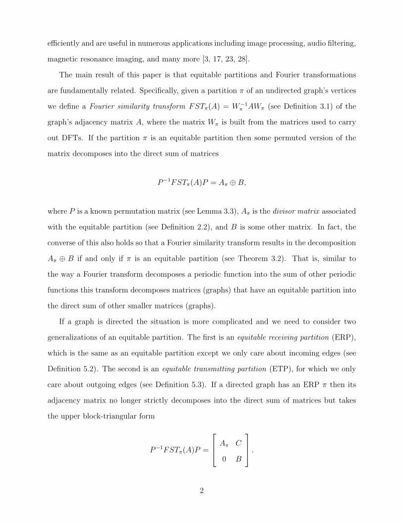
The main result of this paper is that equitable partitions and Fourier transformations

are fundamentally related. Specifically, given a partition π of an undirected graph’s vertices

we define a Fourier similarity transform FSTπ(A) = W−1π AWπ (see Definition 3.1) of the

graph’s adjacency matrix A, where the matrix Wπ is built from the matrices used to carry

out DFTs. If the partition π is an equitable partition then some permuted version of the

matrix decomposes into the direct sum of matrices

P−1FSTπ(A)P = Aπ ⊕B,

where P is a known permutation matrix (see Lemma 3.3), Aπ is the divisor matrix associated

with the equitable partition (see Definition 2.2), and B is some other matrix. In fact, the

converse of this also holds so that a Fourier similarity transform results in the decomposition

Aπ ⊕ B if and only if π is an equitable partition (see Theorem 3.2). That is, similar to

the way a Fourier transform decomposes a periodic function into the sum of other periodic

functions this transform decomposes matrices (graphs) that have an equitable partition into

the direct sum of other smaller matrices (graphs).

If a graph is directed the situation is more complicated and we need to consider two

generalizations of an equitable partition. The first is an equitable receiving partition (ERP),

which is the same as an equitable partition except we only care about incoming edges (see

Definition 5.2). The second is an equitable transmitting partition (ETP), for which we only

care about outgoing edges (see Definition 5.3). If a directed graph has an ERP π then its

adjacency matrix no longer strictly decomposes into the direct sum of matrices but takes

the upper block-triangular form

P−1FSTπ(A)P =

Aπ C

0 B

.

2

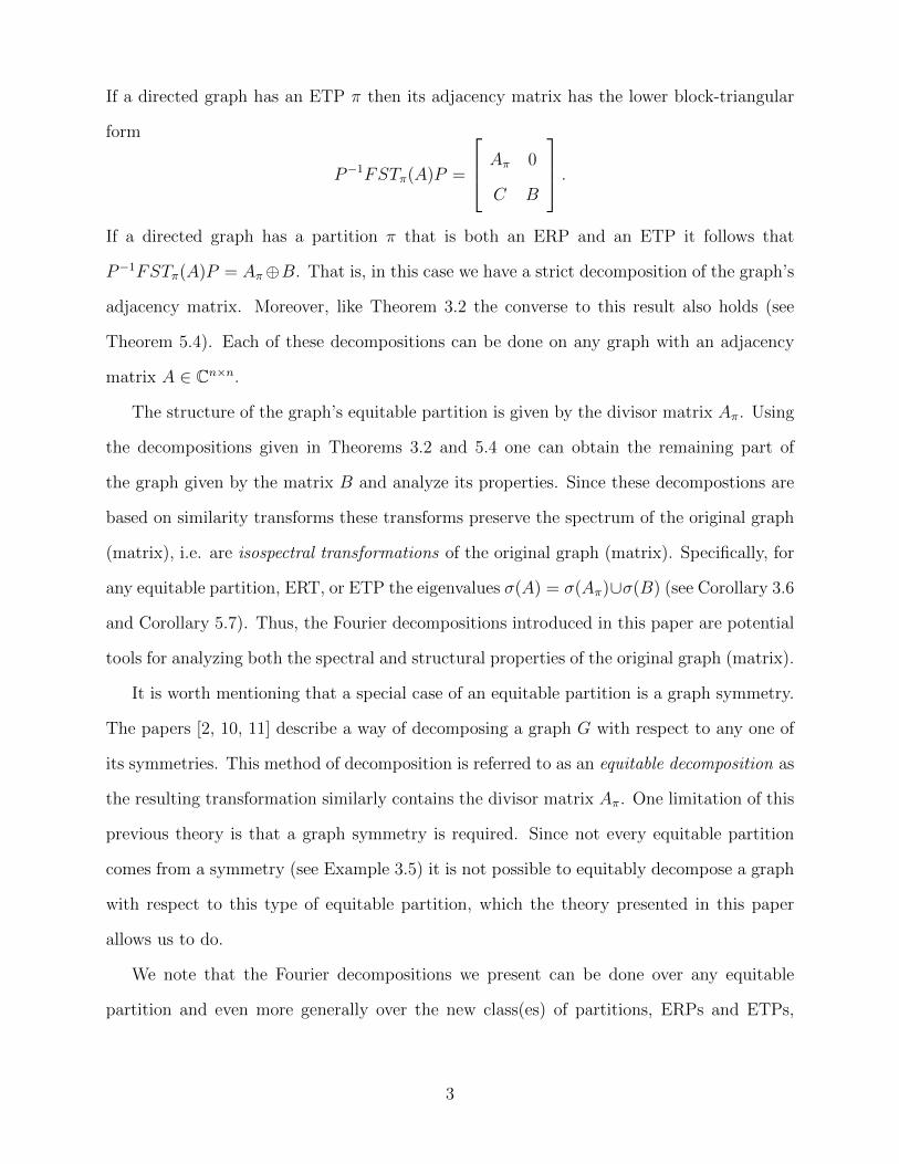
If a directed graph has an ETP π then its adjacency matrix has the lower block-triangular

form

P−1FSTπ(A)P =

Aπ 0

C B

.If a directed graph has a partition π that is both an ERP and an ETP it follows that

P−1FSTπ(A)P = Aπ⊕B. That is, in this case we have a strict decomposition of the graph’s

adjacency matrix. Moreover, like Theorem 3.2 the converse to this result also holds (see

Theorem 5.4). Each of these decompositions can be done on any graph with an adjacency

matrix A ∈ Cn×n.

The structure of the graph’s equitable partition is given by the divisor matrix Aπ. Using

the decompositions given in Theorems 3.2 and 5.4 one can obtain the remaining part of

the graph given by the matrix B and analyze its properties. Since these decompostions are

based on similarity transforms these transforms preserve the spectrum of the original graph

(matrix), i.e. are isospectral transformations of the original graph (matrix). Specifically, for

any equitable partition, ERT, or ETP the eigenvalues σ(A) = σ(Aπ)∪σ(B) (see Corollary 3.6

and Corollary 5.7). Thus, the Fourier decompositions introduced in this paper are potential

tools for analyzing both the spectral and structural properties of the original graph (matrix).

It is worth mentioning that a special case of an equitable partition is a graph symmetry.

The papers [2, 10, 11] describe a way of decomposing a graph G with respect to any one of

its symmetries. This method of decomposition is referred to as an equitable decomposition as

the resulting transformation similarly contains the divisor matrix Aπ. One limitation of this

previous theory is that a graph symmetry is required. Since not every equitable partition

comes from a symmetry (see Example 3.5) it is not possible to equitably decompose a graph

with respect to this type of equitable partition, which the theory presented in this paper

allows us to do.

We note that the Fourier decompositions we present can be done over any equitable

partition and even more generally over the new class(es) of partitions, ERPs and ETPs,

3

introduced here. Moreover, these decompositions are computationally quite simple when

compared to equitable decompositions as they require only a single similarity transform as

opposed to the multiple similarlity transforms required, in general, for an equitable decom-

position (for more details see [2, 10, 11].

In Chapter 2 we describe the basic ideas involving equitable partitions. In Chapter 3

we introduce the notion of a Fourier similarity transform and describe how this transform

can be used to decompose an undirected graph (symmetric matrix) if and only if it has an

equitable partition. In the following chapter we prove this result. In Chapter 5 we generalize

the results of Chapter 3 to directed graphs (general matrices) by introducing the concepts

of equitable receiving and transmitting partitions. In Chapter 6 we discuss the special case

of equitable partitions derived from graph symmetries and connections to the theory of

equitable decompositions. Chapter 7 concludes with a few closing remarks including open

questions regarding Fourier decompositions.

Chapter 2. Equitable Partitions

Graphs are used to represent many types of systems. The key idea that a graph captures

is the structure of relationships or interactions between a collection of objects. The rela-

tionships could be social relationships between individuals, the physical connections between

routers in the Internet, the synapses that couple neurons in the brain, or the interdepen-

dence of variables given by a function F : Rn → Rn. A graph G = (V,E, ω) is composed of

a vertex set V = {1, 2, . . . , n}, an edge set E, and a function ω : E → C used to weight the

edges E of the graph. The vertex set V represents the system’s collection of objects and the

edges E the links or interactions between these objects. The function ω can be though of as

measuring the strength of these interactions. For instance, if the graph represents a social

network the weights might be the frequency of interaction between individuals.

In some systems there is a sense of direction to the system’s set of interactions. For

example, in a citation network, citing a paper is not the same as being cited by a paper.

4

In the graph representing a citation network there is a directed edge from the paper to the

paper it is citing. In this case the graph is a directed graph as every edge has a clearly

defined direction. If the edges of the graph have no specified direction, i.e. are undirected,

then the graph is referred to as an undirected graph. We note that an undirected graph can

be considered to be a directed graph by replacing each of its undirected edges by two directed

edges: one that points from the first to the second vertex and the other that points from the

second back to the first. Hence, any graph can be considered to be a directed graph.

Using this coinvention, let G = (V,E, ω) be a graph on |V | = n vertices. Its adjacency

matrix, A = A(G) ∈ Cn×n has entries given by

Aij =

ω(eij) 6= 0 if eij ∈ E

0 otherwise(2.1)

where eij is the directed edge from vertex i to vertex j. Here an edge eii ∈ E is a loop of the

graph. The eigenvalues of the graph G are the eigenvalues σ(A) of its adjacency matrix. A

graph is undirected if and only if its adjacency matrix is symmetric.

Since ω(eij) ∈ C is the weight of the edge eij the matrix A = A(G) is, technically

speaking, the weighted adjacency matrix of a graph G = (V,E, ω). For simplicity we will

refer to A as the graph’s adjacency matrix. The reason for this is that an unweighted graph

G = (V,E) can be considered to be a special case of a weighted graph where the unweighted

edges of the graph are given unit weight. Without loss in generality then, Equation (2.1)

defines the adjacency matrix for any graph whether it is directed or undirected, weighted or

unweighted.

Despite the generality in which we have defined a graph a large fraction of real-world

systems are represented by simple graphs, which are unweighted, undirected graphs without

loops. This includes, for example, the large majority of networks studied in the social,

technological, and natural sciences [6, 21, 26]. The adjacency matrix of a simple graph

is a symmetric, zero-one matrix, that has an all-zero diagonal. For example, the graph

5

Out[220]=

G

1 2

5 4

7 8

3 6A =

0 0 1 0 1 0 1 00 0 0 1 0 1 0 11 0 0 0 0 1 0 00 1 0 0 0 0 0 11 0 0 0 0 0 1 00 1 1 0 0 0 0 01 0 0 0 1 0 0 00 1 0 1 0 0 0 0

Aπ =

[0 31 1

]Gπ

1 2

31

1

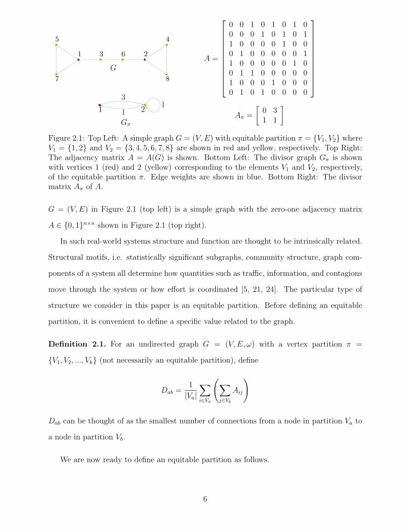
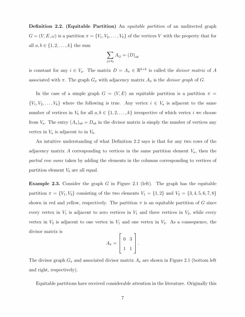
Figure 2.1: Top Left: A simple graph G = (V,E) with equitable partition π = {V1, V2} whereV1 = {1, 2} and V2 = {3, 4, 5, 6, 7, 8} are shown in red and yellow, respectively. Top Right:The adjacency matrix A = A(G) is shown. Bottom Left: The divisor graph Gπ is shownwith vertices 1 (red) and 2 (yellow) corresponding to the elements V1 and V2, respectively,of the equitable partition π. Edge weights are shown in blue. Bottom Right: The divisormatrix Aπ of A.

G = (V,E) in Figure 2.1 (top left) is a simple graph with the zero-one adjacency matrix

A ∈ {0, 1}n×n shown in Figure 2.1 (top right).

In such real-world systems structure and function are thought to be intrinsically related.

Structural motifs, i.e. statistically significant subgraphs, community structure, graph com-

ponents of a system all determine how quantities such as traffic, information, and contagions

move through the system or how effort is coordinated [5, 21, 24]. The particular type of

structure we consider in this paper is an equitable partition. Before defining an equitable

partition, it is convenient to define a specific value related to the graph.

Definition 2.1. For an undirected graph G = (V,E, ω) with a vertex partition π =

{V1, V2, ..., Vk} (not necessarily an equitable partition), define

Dab =1

|Va|∑i∈Va

(∑j∈Vb

Aij

)

Dab can be thought of as the smallest number of connections from a node in partition Va to

a node in partition Vb.

We are now ready to define an equitable partition as follows.

6

Definition 2.2. (Equitable Partition) An equitable partition of an undirected graph

G = (V,E, ω) is a partition π = {V1, V2, . . . , Vk} of the vertices V with the property that for

all a, b ∈ {1, 2, . . . , k} the sum ∑j∈Vb

Aij = (D)ab

is constant for any i ∈ Va. The matrix D = Aπ ∈ Rk×k is called the divisor matrix of A

associated with π. The graph Gπ with adjacency matrix Aπ is the divisor graph of G.

In the case of a simple graph G = (V,E) an equitable partition is a partition π =

{V1, V2, . . . , Vk} where the following is true. Any vertex i ∈ Va is adjacent to the same

number of vertices in Vb for all a, b ∈ {1, 2, . . . , k} irrespective of which vertex i we choose

from Va. The entry (Aπ)ab = Dab in the divisor matrix is simply the number of vertices any

vertex in Va is adjacent to in Vb.

An intuitive understanding of what Definition 2.2 says is that for any two rows of the

adjacency matrix A corresponding to vertices in the same partition element Va, then the

partial row sums taken by adding the elements in the columns corresponding to vertices of

partition element Vb are all equal.

Example 2.3. Consider the graph G in Figure 2.1 (left). The graph has the equitable

partition π = {V1, V2} consisting of the two elements V1 = {1, 2} and V2 = {3, 4, 5, 6, 7, 8}

shown in red and yellow, respectively. The partition π is an equitable partition of G since

every vertex in V1 is adjacent to zero vertices in V1 and three vertices in V2, while every

vertex in V2 is adjacent to one vertex in V1 and one vertex in V2. As a consequence, the

divisor matrix is

Aπ =

0 3

1 1

.The divisor graph Gπ and associated divisor matrix Aπ are shown in Figure 2.1 (bottom left

and right, respectively).

Equitable partitions have received considerable attention in the literature. Originally this

7

interest was due to the spectral properties preserved by these partitions. Likely the most

well-known of these is that if Aπ is a divisor matrix of A then σ(Aπ) ⊆ σ(A) [9, 13]. More

recently equitable partitions have been shown to be a hallmark of real-world networks [19].

Equitable partitions can also have an impact on the function and processes that can take

place on these networks. This includes the formation of synchronizing clusters in dynamical

network models [22, 27, 25]. Additionally, as discussed in Chapter 6, equitable partitions

have been used to decompose graphs with symmetries [2, 10, 11].

In the following chapter we describe how Fourier transformations can be used to decom-

pose a graph into a number of smaller graphs if the graph has an equitable partition.

Chapter 3. Fourier Transforms and Series

The standard use of a Fourier transform is to take a periodic function f : [0, T ] → R

with period T and decompose it into a sum of simple waves given by sines and cosines

or more generally complex exponentials [14]. In particular, it is possible to transform a

square-integrable function f ∈ L2([0, T ],R) into its Fourier series

f(t) =∞∑

k=−∞

cke2πi( k

T)t (3.1)

where

ck =1

T

∫ T

0

f(t)e−2πi(kT)tdt. (3.2)

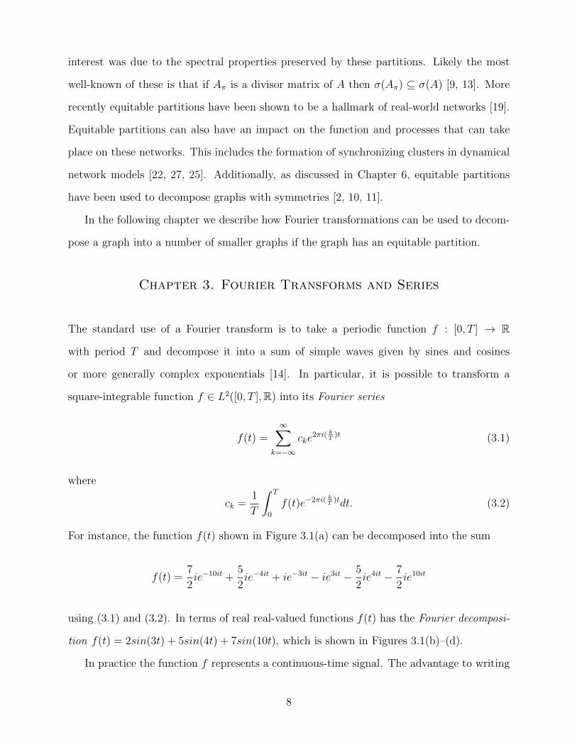
For instance, the function f(t) shown in Figure 3.1(a) can be decomposed into the sum

f(t) =7

2ie−10it +

5

2ie−4it + ie−3it − ie3it − 5

2ie4it − 7

2ie10it

using (3.1) and (3.2). In terms of real real-valued functions f(t) has the Fourier decomposi-

tion f(t) = 2sin(3t) + 5sin(4t) + 7sin(10t), which is shown in Figures 3.1(b)–(d).

In practice the function f represents a continuous-time signal. The advantage to writing

8

Out[1741]=1 2 3 4 5 6

-10

-5

5

10

1 2 3 4 5 6

-10

-5

5

10

1 2 3 4 5 6

-10

-5

5

10

1 2 3 4 5 6

-10

-5

5

10

(a) f(t) (b) f1(t) (c) f2(t) (d) f3(t)

Figure 3.1: The Fourier decomposition of the continuous time signal f(t) into the sumf(t) =

∑3i=1 fi(t) where f1(t) = 2 sin(3t), f2(t) = 5 sin(4t), and f3(t) = 7 sin(10t).

f as in Equation (3.1) is that this gives us an effective way to analyze, filter, and compress the

original signal. In any technological application signals are discrete rather than continuous.

In order to apply Fourier methods to these continuous signals, these signals are converted

to discrete signals via sampling. A sample of a continuous function f is an n-tuple

x = (f(t1), f(t2), . . . , f(tn)) ∈ Rn

where 0 = t1 < t2 < · · · < tn < tn+1 = T .

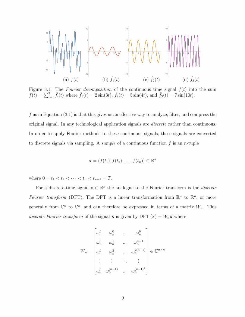
For a discrete-time signal x ∈ Rn the analogue to the Fourier transform is the discrete

Fourier transform (DFT). The DFT is a linear transformation from Rn to Rn, or more

generally from Cn to Cn, and can therefore be expressed in terms of a matrix Wn. This

discrete Fourier transform of the signal x is given by DFT (x) = Wnx where

Wn =

ω0n ω0

n ... ω0n

ω0n ω1

n ... ωn−1n

ω0n ω2

n ... ω2(n−1)n

......

. . ....

ω0n ω

(n−1)n ... ω

(n−1)2n

∈ Cn×n

9

in which ωn is the nth primitive root of unity ωn = e2πi/n. The inverse of this matrix is given

by W−1n = nWH

n = nW where WH is the conjugate transpose of W and W is its conjugate.

Because DFTs can be done efficiently using fast Fourier transforms (FFTs) they are use-

ful in numerous applications including image processing, audio filtering, magnetic resonance

imaging, and many more [3, 17, 23, 28]. To the best of the authors’ knowledge DFTs have

not, however, been used to decompose graphs or matrices. This is potentially because graphs

and matrices are static objects, at least as they are typically defined and there is no obvious

analogy between a sampled signal x ∈ Rn and a graph G with adjacency matrix A ∈ Rn×n.

In what follows, if a graph G = (V,E, ω) has an equitable partition π = {V1, V2, . . . , Vk}

then, without loss in generality, we assume that the vertices of G are numbered such that if

i ∈ Va and j ∈ Vb where a < b then i < j. This amounts to relabelling the vertices of G so

that vertices in the same element of π are labeled consecutively and the vertices in Va precede

those in Va+1 for a = 1, 2, . . . , k−1. For example, the graph G in Figure 2.1 has the equitable

partition π = {V1, V2} that respects this labeling as V1 = {1, 2} and V2 = {3, 4, 5, 6, 7, 8}.

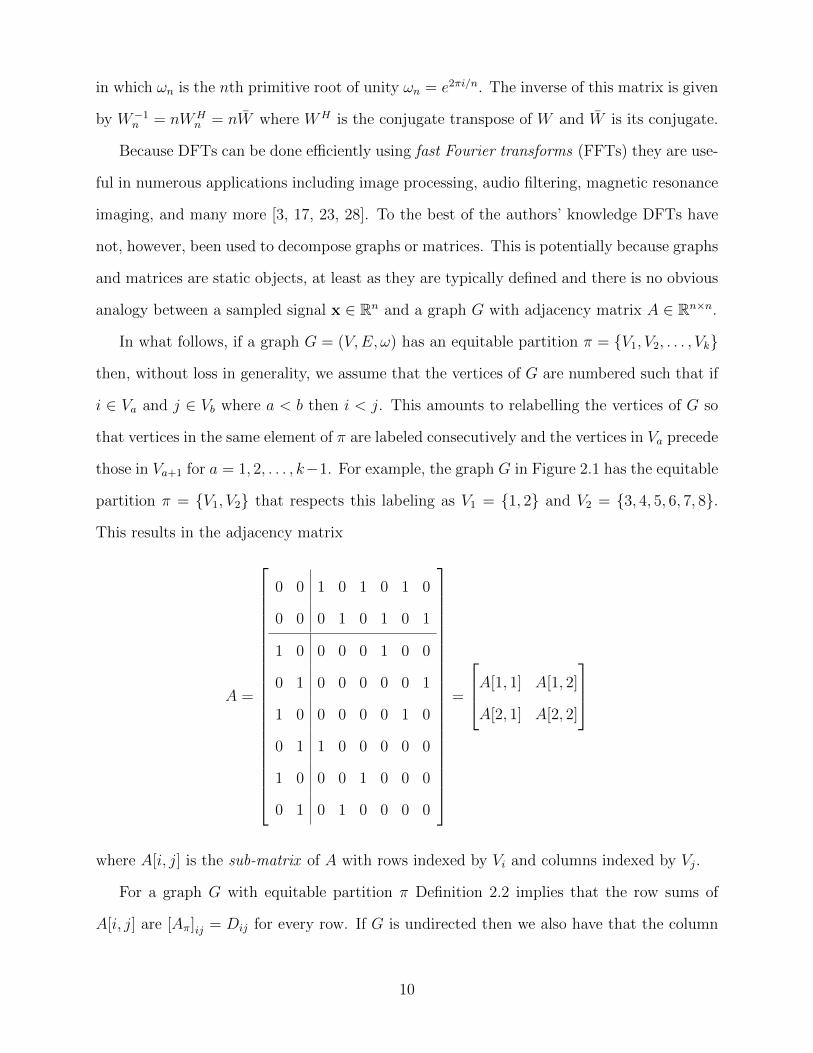
This results in the adjacency matrix

A =

0 0 1 0 1 0 1 0

0 0 0 1 0 1 0 1

1 0 0 0 0 1 0 0

0 1 0 0 0 0 0 1

1 0 0 0 0 0 1 0

0 1 1 0 0 0 0 0

1 0 0 0 1 0 0 0

0 1 0 1 0 0 0 0

=

A[1, 1] A[1, 2]

A[2, 1] A[2, 2]

where A[i, j] is the sub-matrix of A with rows indexed by Vi and columns indexed by Vj.

For a graph G with equitable partition π Definition 2.2 implies that the row sums of

A[i, j] are [Aπ]ij = Dij for every row. If G is undirected then we also have that the column

10

sums of A[i, j] are [Aπ]ji = Dji for every column. This observation will be important in using

Fourier transforms to decompose undirected graphs, i.e. graph whose adjacency matrix is

symmetric (see Theorem 3.2).

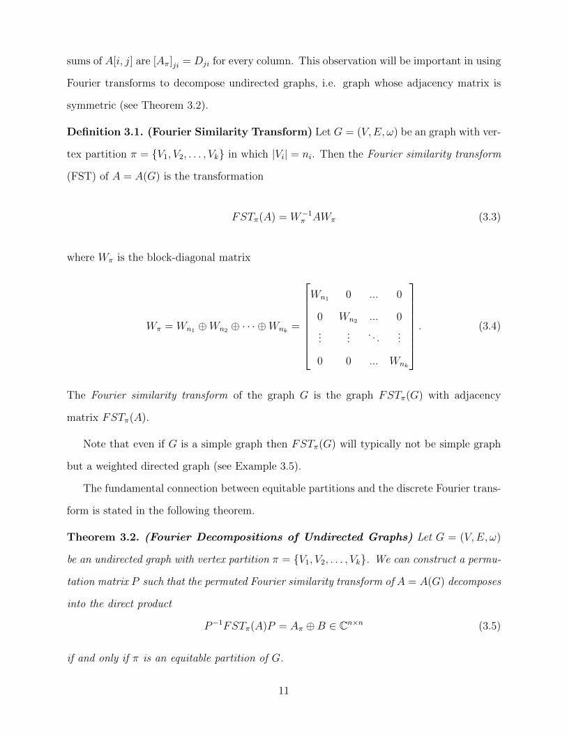
Definition 3.1. (Fourier Similarity Transform) Let G = (V,E, ω) be an graph with ver-

tex partition π = {V1, V2, . . . , Vk} in which |Vi| = ni. Then the Fourier similarity transform

(FST) of A = A(G) is the transformation

FSTπ(A) = W−1π AWπ (3.3)

where Wπ is the block-diagonal matrix

Wπ = Wn1 ⊕Wn2 ⊕ · · · ⊕Wnk=

Wn1 0 ... 0

0 Wn2 ... 0

......

. . ....

0 0 ... Wnk

. (3.4)

The Fourier similarity transform of the graph G is the graph FSTπ(G) with adjacency

matrix FSTπ(A).

Note that even if G is a simple graph then FSTπ(G) will typically not be simple graph

but a weighted directed graph (see Example 3.5).

The fundamental connection between equitable partitions and the discrete Fourier trans-

form is stated in the following theorem.

Theorem 3.2. (Fourier Decompositions of Undirected Graphs) Let G = (V,E, ω)

be an undirected graph with vertex partition π = {V1, V2, . . . , Vk}. We can construct a permu-

tation matrix P such that the permuted Fourier similarity transform of A = A(G) decomposes

into the direct product

P−1FSTπ(A)P = Aπ ⊕B ∈ Cn×n (3.5)

if and only if π is an equitable partition of G.

11

That is, a graph (matrix) can be decomposed into (the direct sum of) a number of smaller

graphs (matrices) via a Fourier similarity transform only in the case that it has an equitable

partition. The proof of Theorem 3.2 is given in the following chapter. To prove this theorem

we use the following lemma, which describes how to construct the permutation matrix P .

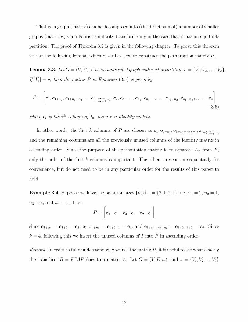
Lemma 3.3. Let G = (V,E, ω) be an undirected graph with vertex partition π = {V1, V2, . . . , Vk}.

If |Vi| = ni then the matrix P in Equation (3.5) is given by

P =

[e1, e1+n1 , e1+n1+n2 , ..., e1+∑k−1

i=1 ni, e2, e3, . . . , en1 , en1+2, . . . , en1+n2 , en1+n2+2, . . . , en

](3.6)

where ei is the ith column of In, the n× n identity matrix.

In other words, the first k columns of P are chosen as e1, e1+n1 , e1+n1+n2 , ..., e1+∑k−1

i=1 ni

and the remaining columns are all the previously unused columns of the identity matrix in

ascending order. Since the purpose of the permutation matrix is to separate Aπ from B,

only the order of the first k columns is important. The others are chosen sequentially for

convenience, but do not need to be in any particular order for the results of this paper to

hold.

Example 3.4. Suppose we have the partition sizes {ni}4i=1 = {2, 1, 2, 1}, i.e. n1 = 2, n2 = 1,

n3 = 2, and n4 = 1. Then

P =

[e1 e3 e4 e6 e2 e5

]since e1+n1 = e1+2 = e3, e1+n1+n2 = e1+2+1 = e4, and e1+n1+n2+n3 = e1+2+1+2 = e6. Since

k = 4, following this we insert the unused columns of I into P in ascending order.

Remark. In order to fully understand why we use the matrix P , it is useful to see what exactly

the transform B = P TAP does to a matrix A. Let G = (V,E, ω), and π = {V1, V2, ..., Vk}

12

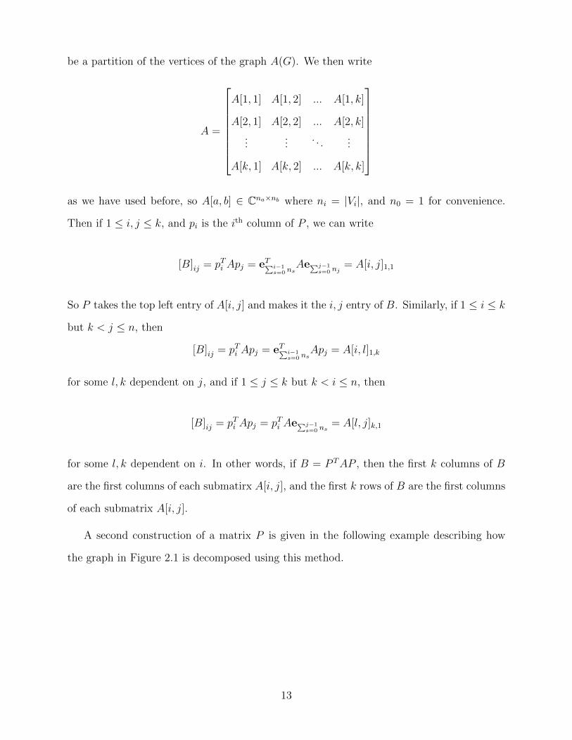
be a partition of the vertices of the graph A(G). We then write

A =

A[1, 1] A[1, 2] ... A[1, k]

A[2, 1] A[2, 2] ... A[2, k]

......

. . ....

A[k, 1] A[k, 2] ... A[k, k]

as we have used before, so A[a, b] ∈ Cna×nb where ni = |Vi|, and n0 = 1 for convenience.

Then if 1 ≤ i, j ≤ k, and pi is the ith column of P , we can write

[B]ij = pTi Apj = eT∑i−1s=0 ns

Ae∑j−1s=0 nj

= A[i, j]1,1

So P takes the top left entry of A[i, j] and makes it the i, j entry of B. Similarly, if 1 ≤ i ≤ k

but k < j ≤ n, then

[B]ij = pTi Apj = eT∑i−1s=0 ns

Apj = A[i, l]1,k

for some l, k dependent on j, and if 1 ≤ j ≤ k but k < i ≤ n, then

[B]ij = pTi Apj = pTi Ae∑j−1s=0 ns

= A[l, j]k,1

for some l, k dependent on i. In other words, if B = P TAP , then the first k columns of B

are the first columns of each submatirx A[i, j], and the first k rows of B are the first columns

of each submatrix A[i, j].

A second construction of a matrix P is given in the following example describing how

the graph in Figure 2.1 is decomposed using this method.

13

Out[262]=

1 2 3

4

56 78

3

11

FSTπ(G)

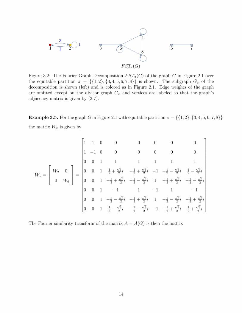
Figure 3.2: The Fourier Graph Decomposition FSTπ(G) of the graph G in Figure 2.1 overthe equitable partition π = {{1, 2}, {3, 4, 5, 6, 7, 8}} is shown. The subgraph Gπ of thedecomposition is shown (left) and is colored as in Figure 2.1. Edge weights of the graphare omitted except on the divisor graph Gπ and vertices are labeled so that the graph’sadjacency matrix is given by (3.7).

Example 3.5. For the graphG in Figure 2.1 with equitable partition π = {{1, 2}, {3, 4, 5, 6, 7, 8}}

the matrix Wπ is given by

Wπ =

W2 0

0 W6

=

1 1 0 0 0 0 0 0

1 −1 0 0 0 0 0 0

0 0 1 1 1 1 1 1

0 0 1 12

+√32i −1

2+√32i −1 −1

2−√32i 1

2−√32i

0 0 1 −12

+√32i −1

2−√32i 1 −1

2+√32i −1

2−√32i

0 0 1 −1 1 −1 1 −1

0 0 1 −12−√32i −1

2+√32i 1 −1

2−√32i −1

2+√32i

0 0 1 12−√32i −1

2−√32i −1 −1

2+√32i 1

2+√32i

The Fourier similarity transform of the matrix A = A(G) is then the matrix

14

FSTπ(A) =

0 0 3 0 0 0 0 0

0 0 0 0 0 3 0 0

1 0 1 0 0 0 0 0

0 0 0 −23

0 −23

0 13

0 0 0 0 0 0 1 0

0 1 0 −23

0 13

0 −23

0 0 0 0 1 0 0 0

0 0 0 13

0 −23

0 −23

and the permutation matrix P is

P =

[e1 e3 e2 e4 e5 e6 e7 e8

],

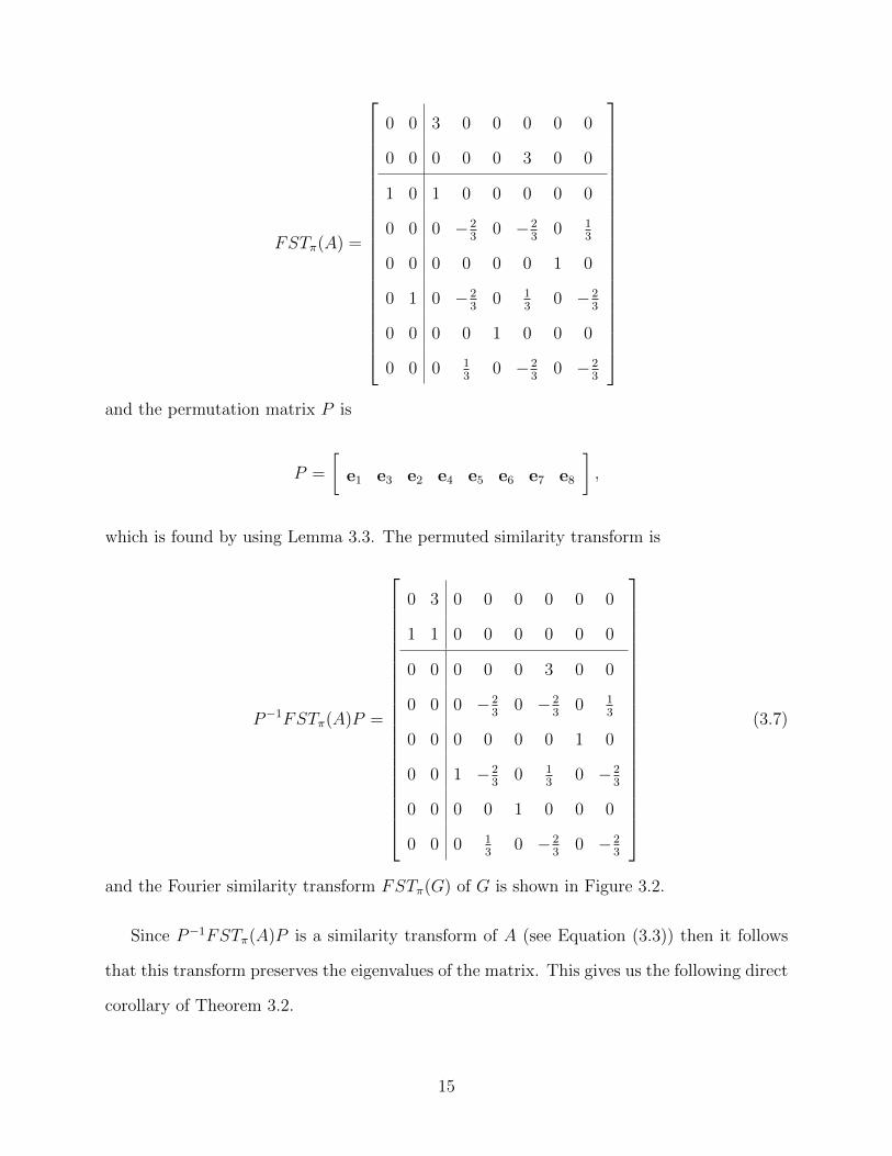
which is found by using Lemma 3.3. The permuted similarity transform is

P−1FSTπ(A)P =

0 3 0 0 0 0 0 0

1 1 0 0 0 0 0 0

0 0 0 0 0 3 0 0

0 0 0 −23

0 −23

0 13

0 0 0 0 0 0 1 0

0 0 1 −23

0 13

0 −23

0 0 0 0 1 0 0 0

0 0 0 13

0 −23

0 −23

(3.7)

and the Fourier similarity transform FSTπ(G) of G is shown in Figure 3.2.

Since P−1FSTπ(A)P is a similarity transform of A (see Equation (3.3)) then it follows

that this transform preserves the eigenvalues of the matrix. This gives us the following direct

corollary of Theorem 3.2.

15

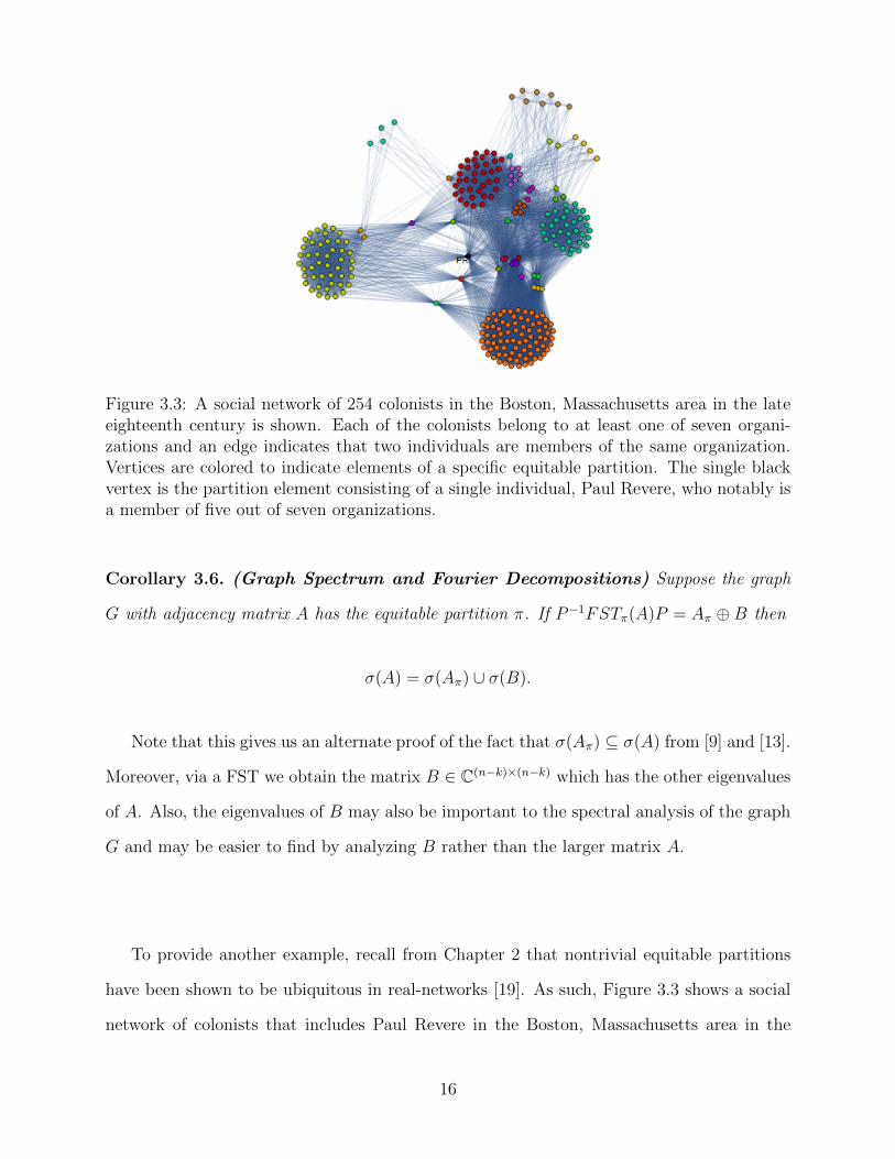
Figure 3.3: A social network of 254 colonists in the Boston, Massachusetts area in the lateeighteenth century is shown. Each of the colonists belong to at least one of seven organi-zations and an edge indicates that two individuals are members of the same organization.Vertices are colored to indicate elements of a specific equitable partition. The single blackvertex is the partition element consisting of a single individual, Paul Revere, who notably isa member of five out of seven organizations.

Corollary 3.6. (Graph Spectrum and Fourier Decompositions) Suppose the graph

G with adjacency matrix A has the equitable partition π. If P−1FSTπ(A)P = Aπ ⊕B then

σ(A) = σ(Aπ) ∪ σ(B).

Note that this gives us an alternate proof of the fact that σ(Aπ) ⊆ σ(A) from [9] and [13].

Moreover, via a FST we obtain the matrix B ∈ C(n−k)×(n−k) which has the other eigenvalues

of A. Also, the eigenvalues of B may also be important to the spectral analysis of the graph

G and may be easier to find by analyzing B rather than the larger matrix A.

To provide another example, recall from Chapter 2 that nontrivial equitable partitions

have been shown to be ubiquitous in real-networks [19]. As such, Figure 3.3 shows a social

network of colonists that includes Paul Revere in the Boston, Massachusetts area in the

16

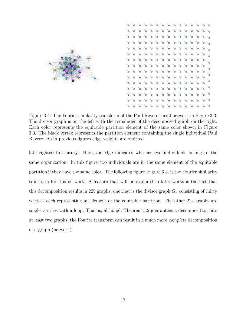
Figure 3.4: The Fourier similarity transform of the Paul Revere social network in Figure 3.3.The divisor graph is on the left with the remainder of the decomposed graph on the right.Each color represents the equitable partition element of the same color shown in Figure3.3. The black vertex represents the partition element containing the single individual PaulRevere. As in previous figures edge weights are omitted.

late eighteenth century. Here, an edge indicates whether two individuals belong to the

same organization. In this figure two individuals are in the same element of the equitable

partition if they have the same color. The following figure, Figure 3.4, is the Fourier similarity

transform for this network. A feature that will be explored in later works is the fact that

this decomposition results in 225 graphs, one that is the divisor graph Gπ consisting of thirty

vertices each representing an element of the equitable partition. The other 224 graphs are

single vertices with a loop. That is, although Theorem 3.2 guarantees a decomposition into

at least two graphs, the Fourier transform can result in a much more complete decomposition

of a graph (network).

17

Chapter 4. Proof of the Graph Decomposi-

tion Theorem

In this chapter we give a proof of Theorem 3.2. Before doing so we require the following

lemma.

Lemma 4.1. If an undirected graph G = (V,E, ω) has adjacency matrix A and an equitable

partition π = {V1, V2, . . . , Vk} such that∑

j∈Vb Aij = Dab for any i ∈ Va, then∑

i∈Va Aij =

Dba for any j ∈ Vb.

Proof. Since G is an undriected graph, then A = AT . Thus, for any j ∈ Vb

∑i∈Va

Aij =∑i∈Va

Aji = Dba.

A useful way to think about Lemma 4.1 is that in an undirected graph every connection

from a vertex in Va to a vertex in Vb is also a connection from a vertex in Vb to a vertex in Va.

If the partial row sums are equal, then, since A is symmetric, it must also be true that the

partial column sums are equal. This is because the partial column sums of A are the partial

row sums of AT = A. The reason for this lemma will become clear by comparing Theorem

3.2 with Theorem 5.4 where we extend the result of Theorem 3.2 to directed graphs.

With Lemma 4.1 in place we provide a proof of Theorem 3.2, which also gives a proof of

Lemma 3.3.

Proof. Let G = (V,E, ω) be an undirected graph with adjacency matrix A ∈ Cn×n. Also, let

π = {V1, ..., Vk} be a partition of the vertices V of the graph G. We also assume the labeling

of the graph verticies is consistent with our previous convention. Namely, that if vx ∈ Vi

and vy ∈ Vj with i < j, then x < y for all 1 ≤ x, y ≤ n and 1 ≤ i, j ≤ k. Finally, we also use

π and G to define P as in Lemma 3.3, and let |Vi| = ni.

18

Using the notation A[a, b], introduced in Chapter 3 we write A as

A =

A[1, 1] A[1, 2] A[1, 3] . . . A[1, k]

A[2, 1] A[2, 2] A[2, 3] . . . A[2, k]

A[3, 1] A[3, 2] A[3, 3] . . . A[3, k]

......

.... . .

...

A[k, 1] A[k, 2] A[k, 3] . . . A[k, k]

.

where A[a, b] ∈ Cna×nb corresponding to the partition π. We then have

FSTπ(A) = W−1π AWπ =

1n1WHn1A[1, 1]Wn1

1n1WHn1A[1, 2]Wn2 . . . 1

n1WHn1A[1, k]Wnk

1n2WHn2A[2, 1]Wn1

1n2WHn2A[2, 2]Wn2 . . . 1

n2WHn2A[2, k]Wnk

......

. . ....

1nkWHnkA[k, 1]Wn1

1nkWHnkA[k, 2]Wn2 . . . 1

nkWHnkA[k, k]Wnk

in which FSTπ(A)[a, b] = 1

naWHnaA[a, b]Wnb

.

Note that the permutation matrix P described in Lemma 3.3 takes the first row and

column of each block 1naWHnaA[a, b]Wnb

and moves it to the ath row and bth column (see

Remark 3). Hence, the statement

P−1FSTπ(A)P = A⊕B (4.1)

is equivalent to saying that for each block 1naWHnaA[a, b]Wnb

, the top left entry is some constant

(for now, we will use a placeholder value dependent on a and b, called aab), and every other

entry in either the first row or first column is 0. That is,

[1

naWHnaA[a, b]Wnb

]xy

=

aab for x = y = 1

0 for x 6= y = 1 or y 6= x = 1.

(4.2)

Our goal is to show that Equation (4.2) holds if and only if π is an equitable partition.

19

Assume then that π is an equitable partition. Then the partial row sum∑

j∈Vb Aij = Dab

is constant for any i ∈ Va with a fixed. Thus,

[1

naWHnaA[a, b]Wnb

]xy

=1

na

na∑s=1

nb∑t=1

cstω(x−1)(s−1)na

ω(y−1)(t−1)nb

where [A[a, b]]st = cst. When x = y = 1 we have

[1

naWHnaA[a, b]Wnb

]11

=1

na

na∑s=1

nb∑t=1

cstω0naω0nb

=1

na

na∑s=1

nb∑t=1

cst. (4.3)

Because π is an equitable partition, our labeling assumption gives us that every s involved

in this sum relates to a vertex vi ∈ Va. Thus,

nb∑t=1

cst =

nb∑t=1

[A[a, b]]st =∑j∈Vb

Aij = Dab

for every choice of i ∈ Va, or rather, for each s. Thus

[1

naWHnaA[a, b]Wnb

]11

=1

na

na∑s=1

(nb∑t=1

cst

)=

1

na

na∑s=1

Dab = Dab

so that Equation (4.2) holds in the case that x = y = 1.

In the case that x 6= 1, and y = 1 we have,

[1

naWHnaA[a, b]Wnb

]x1

=1

na

na∑s=1

nb∑t=1

cstω(x−1)(s−1)na

ω0nb

=1

na

na∑s=1

nb∑t=1

cstω(x−1)(s−1)na

=1

na

na∑s=1

ω(x−1)(s−1)na

(nb∑t=1

cst

)

=

(Dab

na

) na∑s=1

ω(x−1)(s−1)na

(by Definition 2.2)

=

(Dab

na

)(0)

= 0.

20

When we look at the x = 1 and y 6= 1 case, we get

[1

naWHnaA[a, b]Wnb

]1y

=1

na

na∑s=1

nb∑t=1

cstω0naω(y−1)(t−1)nb

=1

na

na∑s=1

nb∑t=1

cstω(y−1)(t−1)nb

=1

na

nb∑t=1

ω(y−1)(t−1)nb

(na∑s=1

cst

)

=

(Dba

na

) nb∑t=1

ω(y−1)(t−1)nb

(by Lemma 4.1)

=

(Dba

na

)(0)

= 0.

These cases together imply that Equation (4.2) holds when either x 6= 1 and y = 1 or x = 1

and y 6= 1. Hence, Equation (4.2) holds implying P−1FSTπ(A)P = Aπ ⊕B as desired.

Conversely, suppose now that P−1FSTπ(A)P = A ⊕ B for the vertex partition π, or

rather that the matrix FSTπ(A) = W−1π AWπ has the property that

[1

naWHnaA[a, b]Wnb

]xy

=

aab for x = y = 1

0 for x 6= y = 1 or y 6= x = 1.

where again, aab is some placeholder value dependent on a and b.

In order to consider the first column of this block of FSTπ(A), we calculate 1naWHnaA[a, b]1nb

,

where 1nbis the vector of all ones of length nb. This is the scalar 1

natimes the row

sums of WHnaA[a, b] = H. An arbitrary element of H is then calculated to be Hxy =∑na

s=1 ω(x−1)(s−1)na csy, and thus the xth row sum of H is

nb∑t=1

(na∑s=1

ω(x−1)(s−1)na

cst

)=

na∑s=1

[ω(x−1)(s−1)na

(nb∑t=1

cst

)]=

na∑s=1

[ω(x−1)(s−1)na

Rs

]where Rs =

∑nb

t=1 cst =∑

j∈Vb Aij for all i ∈ Va is the partial row sum of A. This is equivalent

21

to the statement thatnb∑t=1

Hxt =na∑s=1

[ω(x−1)(s−1)na

Rs

]= 0

for x = 2, ..., na, which can be written in matrix form as

Zc =

ω0na

ω−1na... ω

−(na−1)na

ω0na

ω−2na... ω

−2(na−1)na

......

. . ....

ω0na

ω−(na−1)na .. ω

−(na−1)2na

R1

R2

...

Rna

= 0.

Note that Z is the inverse of the na × na discrete Fourier transform Wna with the first

row removed. This means that the dimension of the row space of Z is na − 1 implying that

the null space of Z has dimension 1. Observe that c = 1na is in the null space of Z, and

as such Null(Z) = q1na for q ∈ R, implying Ri = Rj for all 1 ≤ i, j ≤ na, so∑

j∈Vb Aij is

constant ∀i ∈ VA. Hence, the partial row sums of the adjacency matrix corresponding to π

are equal and Dab = 1na

∑i∈Va

(∑j∈Vb Aij

)=∑

j∈Vb Aij = Rl for all 1 ≤ l ≤ na, making π

an equitable partition.

Remark. The fact that the first row of each A[a, b] block, except for the row’s first element,

is 0 is not explicitly used in either direction of the proof. However, since we are dealing with

only undirected graphs at this stage, our condition that the first column of A[a, b] (excepting

its first element) is 0 necessarily means that the first row of A[a, b] follow the same pattern.

This detail is explained further in Chapter 5 where Theorem 3.2 is extended to directed

graphs.

22

Chapter 5. Generalization of Equitable De-

compositions to Directed Graphs and

Consequences

Our previous definition of an equitable partition was specific to undirected graphs (see Def-

inition 2.2). To extend this concept to directed graphs we define two new types of equitable

partitions. Again, for convenience, we define two values to assist us.

Definition 5.1. Let G = (V,E, ω) be a directed graph with partition π = {V1, V2, ..., Vk} of

the vertices V . Define

Rab =1

na

∑i∈Va

(∑j∈Vb

Aij

)

and

Tab =1

nb

∑j∈Vb

(nbna

∑i∈Va

Aij

)=

1

na

∑j∈Vb

(∑i∈Va

Aij

)

Note that Rab and Tab are anologues to Dab but for directed graphs.

Definition 5.2 (Equitable Receiving Partition). An equitable receiving partition (ERP)

of a graphG = (V,E, ω) is a partition π = {V1, V2, . . . , Vk} of the vertices V with the property

that for all a, b ∈ {1, 2, . . . , k} the sum

∑j∈Vb

Aij = Rab

is constant for any i ∈ Va. The matrix Aπ = R is the (receiving) divisor matrix of A with

respect to π and Gπ is the (receiving) divisor graph with adjacency matrix Aπ.

Definition 5.2 is, in fact, the same as our original definition of an equitable partition with

the exception that an ERP is not restricted only to undirected graphs. If a graph G has

an ERP then the partial row sums of its adjacency matrix within each partition element is

constant. For the graph G this means that every vertex i ∈ Va receives the same total input,

i.e. sum of weights, from any other partition element Vb.

23

Definition 5.3 (Equitable Transmitting Partition). An equitable transmitting partition

(ETP) of a graph G = (V,E, ω) is a partition π = {V1, V2, . . . , Vk} of the vertices V with the

property that for all a, b ∈ {1, 2, . . . , k} the sum

∑i∈Va

Aij =nanbTab

is constant for any j ∈ Vb. The matrix Aπ = T is the (transmitting) divisor matrix of A

with respect to π and Gπ is the (transmitting) divisor graph with adjacency matrix Aπ.

The difference between an ETP and an ERP is that an ERP has constant partial row

sums within partition elements, while the ETP has constant partial column sums. For the

graph G this is equivalent to saying that every vertex j ∈ Vb sends the same total output,

i.e. sum of weights, to any other partition element Va.

We note that if an undirected graph G has an equitable partition π, as defined in Chapter

2, then π is both an ERP and an ETP if we consider G to be a directed graph, i.e. each of the

graphs edges is replaced with two directed edges oriented in opposite directions. However,

the converse is not always true. A partition can be both an ERP and an ETP but not an

equitable partition of an undirected graph (see Example 5.5).

24

Theorem 5.4. (Fourier Decompositions of Directed Graphs) Let G = (V,E, ω) be

a directed graph with vertex partition π = {V1, V2, . . . , Vk}. We can construct a permuta-

tion matrix P ∈ {0, 1}n×n such that the permuted discrete Fourier transform of A = A(G)

decomposes into the direct product

P−1FSTπ(A)P = Aπ ⊕B ∈ Cn×n

if and only if π is both an ERP and an ETP of G. Additionally, the matrix FSTπ(A) is

reducible if and only if π is either an ERP or an ETP. Specifically, we can construct a

permutation matrix P such that

P−1FSTπ(A)P =

Aπ C

0 B

(5.1)

if and only if π is an ERP, and

P−1FSTπ(A)P =

Aπ 0

C B

(5.2)

if and only if π is an ETP. We refer to this as a weak decomposition of A since the associated

graph has at least two weakly connected components corresponding to Aπ and B, respectively.

Remark. The permutation matrix P in Theorem 5.4 is the same permutation matrix con-

structed for Theorem 3.2, defined in Lemma 3.3.

Proof. First, we note that proving

P−1FSTπ(A)P =

Aπ C

0 B

25

if and only if π is an ERP and

P−1FSTπ(A)P =

Aπ 0

C B

if and only if π is an ETP necessarily proves that

P−1FSTπ(A)P = Aπ ⊕B

if and only if π is both an ERP and an ETP. As such, we focus on proving Equations (5.1)

and (5.2)

Suppose then that π is an ERP. Note that the definition of an ERP is the same as

the definition of an equitable partition for an undirected graph (see Definition 2.2) where

Rab = Dab for a directed graph. However, the proof of Theorem 3.2 in the specific case that

x 6= 1 and y = 1 does not rely on the fact that G is directed Hence, the argument in the

proof of Theorem 3.2 also proves that Equation (5.1) holds if and only if π is an ERP.

To prove Equation (5.2) holds if and only if π is an ETP we suppose for the moment that

π is an ETP. To prove Equation (5.2) holds we then need to show

[1

naWHnaA[a, b]Wnb

]xy

=

Tab for x = y = 1

0 y 6= x = 1.

If x = y = 1 then

[1

naWHnaA[a, b]Wnb

]11

=1

na

na∑s=1

nb∑t=1

cst =1

na

nb∑t=1

na∑s=1

cst

as in Equation (4.3). Since π is an ETP then

na∑s=1

cst =∑i∈Va

Aij =nanbTab,

26

so that

1

na

nb∑t=1

na∑s=1

cst =1

na

nb∑t=1

(nanbTab

)=

1

nb

nb∑t=1

Tab = Tab.

Now, we look specifically at the x = 1 and y 6= 1 case. The argument is exactly the one

presented in the proof of Theorem 3.2, except it utilizes Definition 5.3 instead of Lemma 4.1.

Thus, if π is an equitable partition then Equation (5.2) holds.

Now assume that Equation (5.2) holds, so that the FSTπ(A) is reducible via the per-

mutation matrix P defined in Lemma 3.3. The argument that π must be an ETP is very

similar to the one provided in the proof of Theorem 3.2. However, there are minor details

that are different. Specifically, in order to consider the first row of 1naWHnaA[a, b]Wnb

we can

look at 1na1TnaA[a, b]Wnb

, which is a scalar times the column sums of A[a, b]Wnb= F . Using

the same notation as before, an arbitrary element of F is calculated as

Fxy =

nb∑t=1

cxtω(t−1)(y−1)nb

,

and thus the yth column sum of F is

na∑s=1

(nb∑t=1

cstω(t−1)(y−1)nb

)=

nb∑t=1

[ω(t−1)(y−1)nb

(na∑s=1

cst

)]=

nb∑t=1

[ω(t−1)(y−1)nb

Ct]

where Ct =∑na

s=1 cst =∑

i∈Va Aij for all j ∈ Vb, or rather, for every t. Equation 5.2 then

givesna∑s=1

Fsy =

nb∑t=1

[ω(t−1)(y−1)nb

Ct]

= 0

for y = 2, ..., nb. Which we write as a system of equations in matrix form as

Zc =

ω0nb

ω1nb

... ωnb−1nb

ω0nb

ω2nb

... ω2(nb−1)nb

......

. . ....

ω0nb

ωnb−1nb

... ω(nb−1)2nb

C1

C2

...

Cnb

= 0.

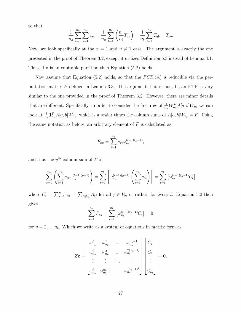
27

Similar to before, Z is the nb × nb discrete Fourier transform with the first row removed

so the rows of Z are linearly independent. Thus the row space of Z has dimension nb − 1

implying that the null space of Z has dimension 1. Once again, c = 1nb∈ Null(Z),

and so Null(Z) = q1m for q ∈ R, which implies that Ci = Cj for all 1 ≤ i, j ≤ nb, so∑i∈Va Aij is constant for all j ∈ Vb. Hence, the partial column sums of the adjacency matrix

corresponding to π are equal making π an equitable transmitting partition.

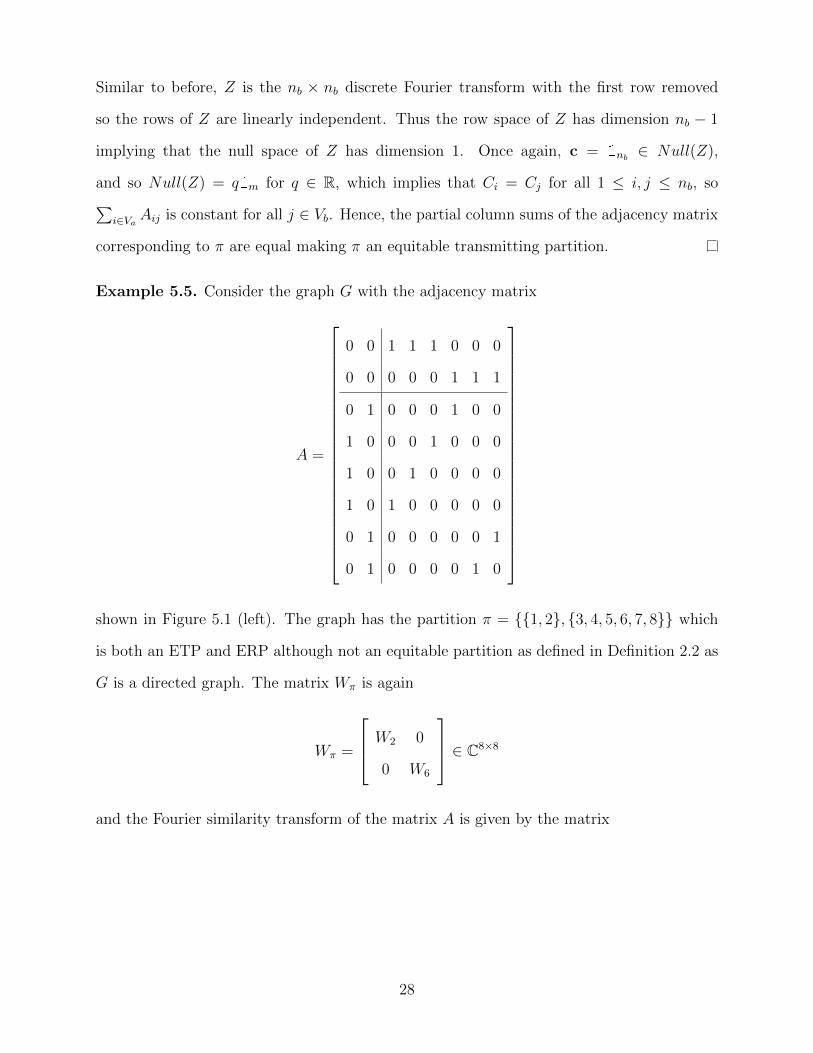
Example 5.5. Consider the graph G with the adjacency matrix

A =

0 0 1 1 1 0 0 0

0 0 0 0 0 1 1 1

0 1 0 0 0 1 0 0

1 0 0 0 1 0 0 0

1 0 0 1 0 0 0 0

1 0 1 0 0 0 0 0

0 1 0 0 0 0 0 1

0 1 0 0 0 0 1 0

shown in Figure 5.1 (left). The graph has the partition π = {{1, 2}, {3, 4, 5, 6, 7, 8}} which

is both an ETP and ERP although not an equitable partition as defined in Definition 2.2 as

G is a directed graph. The matrix Wπ is again

Wπ =

W2 0

0 W6

∈ C8×8

and the Fourier similarity transform of the matrix A is given by the matrix

28

Out[2897]=

3

11

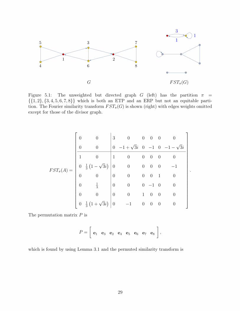
FSTπ(G)G

1 2

5

4

7

8

3

6

Figure 5.1: The unweighted but directed graph G (left) has the partition π ={{1, 2}, {3, 4, 5, 6, 7, 8}} which is both an ETP and an ERP but not an equitable parti-tion. The Fourier similarity transform FSTπ(G) is shown (right) with edges weights omittedexcept for those of the divisor graph.

FSTπ(A) =

0 0 3 0 0 0 0 0

0 0 0 −1 +√

3i 0 −1 0 −1−√

3i

1 0 1 0 0 0 0 0

0 13

(1−√

3i)

0 0 0 0 0 −1

0 0 0 0 0 0 1 0

0 13

0 0 0 −1 0 0

0 0 0 0 1 0 0 0

0 13

(1 +√

3i)

0 −1 0 0 0 0

.

The permutation matrix P is

P =

[e1 e3 e2 e4 e5 e6 e7 e8

],

which is found by using Lemma 3.1 and the permuted similarity transform is

29

P−1FSTπ(A)P =

0 3 0 0 0 0 0 0

1 1 0 0 0 0 0 0

0 0 0 −1 +√

3i 0 1 0 −1−√

3i

0 0 13

(1−√

3i)

0 0 0 0 −1

0 0 0 0 0 0 1 0

0 0 13

0 0 −1 0 0

0 0 0 0 1 0 0 0

0 0 13

(1 +√

3i)

−1 0 0 0 0

.

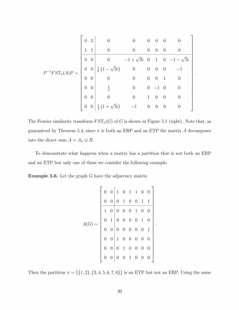
The Fourier similarity transform FSTπ(G) of G is shown in Figure 5.1 (right). Note that, as

guaranteed by Theorem 5.4, since π is both an ERP and an ETP the matrix A decomposes

into the direct sum A = Aπ ⊕B.

To demonstrate what happens when a matrix has a partition that is not both an ERP

and an ETP but only one of these we consider the following example.

Example 5.6. Let the graph G have the adjacency matrix

A(G) =

0 0 1 0 1 1 0 0

0 0 0 1 0 0 1 1

1 0 0 0 0 1 0 0

0 1 0 0 0 0 1 0

0 0 0 0 0 0 0 1

0 0 1 0 0 0 0 0

0 0 0 1 0 0 0 0

0 0 0 0 1 0 0 0

.

Then the partition π = {{1, 2}, {3, 4, 5, 6, 7, 8}} is an ETP but not an ERP. Using the same

30

permutation matrix P as in Example 5.5 the permuted similarity transform is

P−1FSTπ(A)P =

0 3 0 0 0 0 0 0

1 1 0 0 0 0 0 0

0 0 0 −12α−

12β− 1 0 1

112β− 0 1

12α+ −1 0 0 0 0

112α− 0 1

12β+ 0 1 0 0 0

0 0 13

0 0 −1 0 0

112β+ 0 1

12α− 0 0 0 0 −1

112β+

112α− 0 0 0 0 −1

where α± = 1 ±

√3i and β± = 3 ±

√3i, which is block lower-triangular as guaranteed by

Theorem 5.4.

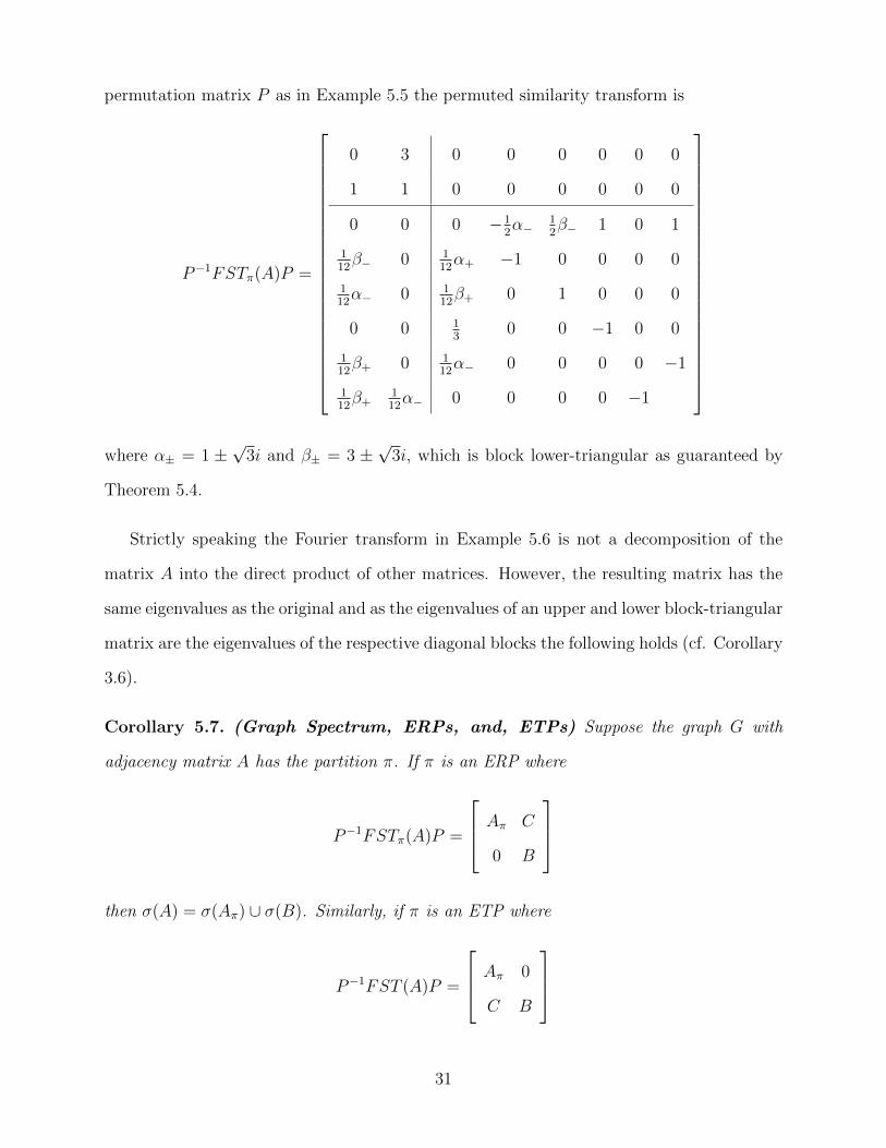
Strictly speaking the Fourier transform in Example 5.6 is not a decomposition of the

matrix A into the direct product of other matrices. However, the resulting matrix has the

same eigenvalues as the original and as the eigenvalues of an upper and lower block-triangular

matrix are the eigenvalues of the respective diagonal blocks the following holds (cf. Corollary

3.6).

Corollary 5.7. (Graph Spectrum, ERPs, and, ETPs) Suppose the graph G with

adjacency matrix A has the partition π. If π is an ERP where

P−1FSTπ(A)P =

Aπ C

0 B

then σ(A) = σ(Aπ) ∪ σ(B). Similarly, if π is an ETP where

P−1FST (A)P =

Aπ 0

C B

31

then σ(A) = σ(Aπ) ∪ σ(B).

Note that, as with standard equitable partitions, this shows that the eigenvalues of the

divisor matrix of an ERP and an ETP are a subset of the adjacency matrix A, i.e. σ(Aπ) ⊂

σ(A).

Chapter 6. Fourier Decompositions over

Symmetries

A special case of an equitable partition is a graph symmetry. In a simple graph G = (V,E) a

symmetry is a permutation φ : V → V of the graph’s vertices that preserves adjacencies, i.e.

preserves each vertex’ neighbors. The permutation φ is called an automorphism of G and

the symmetries of the graph G are the graph’s set of automorphisms. More intuitively, an

automorphism describes how parts of a graph can be interchanged in a way that preserves

the graph’s overall structure. In this sense these parts, i.e., subgraphs, are symmetrical and

together constitute a graph symmetry.

In general, an automorphism of a graph G = (V,E, ω) can be defined as follows.

Definition 6.1. (Graph Automorphism) An automorphism φ of a graph G = (V,E, ω)

is a permutation of V such that the adjacency matrix A = A(G) satisfies

Aij = Aφ(i)φ(j)

for each pair of vertices i and j. The set of all automorphisms of G is a group, denoted by

Aut(G). The order of φ is the smallest positive integer ` = |φ| such that φ` is the identity.

As it turns out, every graph symmetry gives us an equitable partition. The reason is

that given an automorphism φ of the graph the orbit of a vertex v ∈ V is the vertex set

O(v) = {φi(v) : i = 1, 2, . . . , ` for ` = |φ|}.

32

Out[313]=

1 23 45 6

7 8G

13

5

7

2 4

6

8Gπ

FSTπ(G)

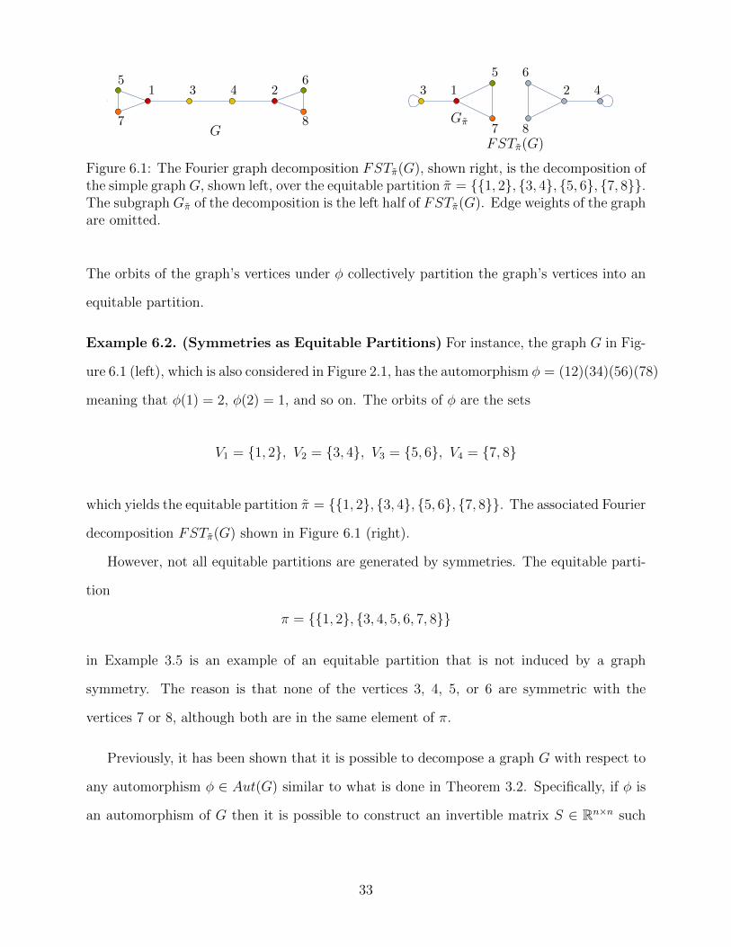
Figure 6.1: The Fourier graph decomposition FSTπ(G), shown right, is the decomposition ofthe simple graph G, shown left, over the equitable partition π = {{1, 2}, {3, 4}, {5, 6}, {7, 8}}.The subgraph Gπ of the decomposition is the left half of FSTπ(G). Edge weights of the graphare omitted.

The orbits of the graph’s vertices under φ collectively partition the graph’s vertices into an

equitable partition.

Example 6.2. (Symmetries as Equitable Partitions) For instance, the graph G in Fig-

ure 6.1 (left), which is also considered in Figure 2.1, has the automorphism φ = (12)(34)(56)(78)

meaning that φ(1) = 2, φ(2) = 1, and so on. The orbits of φ are the sets

V1 = {1, 2}, V2 = {3, 4}, V3 = {5, 6}, V4 = {7, 8}

which yields the equitable partition π = {{1, 2}, {3, 4}, {5, 6}, {7, 8}}. The associated Fourier

decomposition FSTπ(G) shown in Figure 6.1 (right).

However, not all equitable partitions are generated by symmetries. The equitable parti-

tion

π = {{1, 2}, {3, 4, 5, 6, 7, 8}}

in Example 3.5 is an example of an equitable partition that is not induced by a graph

symmetry. The reason is that none of the vertices 3, 4, 5, or 6 are symmetric with the

vertices 7 or 8, although both are in the same element of π.

Previously, it has been shown that it is possible to decompose a graph G with respect to

any automorphism φ ∈ Aut(G) similar to what is done in Theorem 3.2. Specifically, if φ is

an automorphism of G then it is possible to construct an invertible matrix S ∈ Rn×n such

33

that

SAS−1 = Aφ ⊕B (6.1)

where Aφ is the divisor matrix corresponding to the equitable partition induced by φ. The

decompositions given by (6.1) are referred to as equitable decompositions and are described

in a sequence of papers (see [2, 10, 11]).

Initially, the theory of equitable decompositions was limited to decompositions over uni-

form automorphisms or automorphisms in which each nontrivial orbit has the same fixed

size [2] (cf. Example 6.2). The second paper on equitable decompositions extends this to

basic automorphisms in which the order of the automorphism is the product of distinct

primes [10]. Most recently, the theory of equitable decompositions has been extended to any

automorphism φ ∈ Aut(G) of any order [11].

An equitable decomposition of a matrix A with respect to a general automorphism φ is

a more computationally expensive process than performing a FST. If the order of φ has the

prime decomposition

|φ| = p1p2 · · · p`

where each pi is a prime then the equitable decomposition over φ takes ` steps; one for every

prime in |φ|. At each step in the process we need to create a matrix Si ∈ Rn×n. This results

in an equitable decomposition given by a sequence of similarity transforms

S`(· · · (S2(S1AS−11 )S−12 · · · )S−1` = Aφ ⊕B ∈ Rn×n. (6.2)

Each step of the process involves a number of substeps for creating the matrix Si as well as

creating a new automorhpism φi used in the following step to create Si+1.

Although the process shown by Equation (6.2) results in a real decomposition of A,

which may be useful in certain applications, a single step in this process is typically more

complicated, both theoretically and computationally, than the whole of the FST method

introduced in Chapter 3. Moreover, the method of equitable decompositions is, in fact,

34

limited to decompositions over graph symmetries while the method presented in this paper

can be used on any graphs, directed or undirected, weighted or unweighted, that have either

an equitable partition, an ERP, or an ETP.

Chapter 7. Conclusion

As mentioned in Chapter 6, the FST method very much simplifies and otherwise improves

the theory of equitable decompositions. It does so by extending the method of equitable

decompositions that work only with graph symmetries to the more general case of equitable

partitions on directed and undirected graphs.

To handle the directed case we introduce in this paper two new kinds of equitable par-

titions. Namely, equitable receiving partitions and equitable transmitting partitions. We

show that a graph weakly decomposes under a Fourier similarity transform if and only if

the graph has at least one of these partitions, and completely decomposes if and only if it

has a partition that is both an ERP and an ETP simultaneously. We also show that this

method preserves the eigenvalues of the original adjacency matrix, and separates them into

two groups: those that are eigenvalues of the divisor graph, and those that are eigenvalues

of the remainder graph.

Though the Fourier transformations decompositions may not always result in the simplest

decomposition possible, e.g. the decomposition may be complex-valued while others may be

real, the simplicity of the method and the if and only if relationship between the FST and

graph decompositions suggest that there are more connections to be found and many of the

potential applications of the FST method are currently unexplored.

For instance, how thoroughly can a FST decompose a graph? We saw in Example 3.5

that the FST decomposed into two components with real weights, Example 5.5 into two

components with imaginary weights. The Paul Revere network in Figure 3.4 broke into the

divisor graph and 224 isolated vertices. A potentially interesting question is whether it is

possible that every graph can be decomposed as nicely, or will some graphs always have

35

imaginary edges under a Fourier similarity transform? When a graph is decomposed, we are

guaranteed two components (the divisor graph and some remainder) but can we guarantee

any further decomposition as in Figure 3.4?

Another line of questions are related to Fourier theory and signal analysis. What would

it mean for a graph to be decomposed into frequency space, which is a standard notion

in Fourier theory? Are there other applications of signal processing that can be applied

to graphs, such as Kalman Filtering? Could some aspect of signal processing be used to

generate a useful link prediction algorithm in real-world networks, etc.? These are the kind

of questions that we hope to considered in future studies on this topic.

36

Bibliography

[1] A. Balaban, Applications of Graph Theory in Chemistry. Journal of Chemical Informa-

tion and Computer Sciences, 25:334-343, 1985

[2] W. Barret, A. Francis, and B. Webb, Equitable decompositions of graphs with symmetry.

Linear Algebra and its Applications, 513:409 - 434, 2017.

[3] A. Boggess and F. J. Narcowich, A first Course in wavelets with Fourier analysis. John

Wiley & Sons, Hoboken, NJ, second edition, 2009.

[4] D. Bonchev and D.H. Rouvray (Eds.), Chemical Graph Theory: Introduction and Fun-

damentals. Abacus Press, 1991

[5] K.L. Calvert, M.B. Doar, and E.W. Zegura, Modeling Internet Topology. IEEE Commu-

nications Magazine, 35:160-163, 1997.

[6] P. Carrington, J. Scott, and S. Wasserman, Models and Methods in Social Network

Analysis. Cambridge University Press, 2005.

[7] C. Chen, W. Ye, Y. Zuo, C. Zheng, and S. Ping Ong, Graph Networks as a Univer-

sal Machine Learning Framework for Molecules and Crystals. Chemistry of Materials,

31(9):3564-3572, 2019

[8] T. Cormen, C. Leiserson, R. Rivest, C. Stein, Introduction to Algorithms. The MIT

Press, Cambridge, Massachusetts, third edition, 2009.

[9] D. Cvetkovic, P. Rowlinson, and S. Simic, An Introduction to the Theory of Graph

Spectra. London Mathematical Society Student Texts. Cambridge University Press, 2009.

[10] A. Francis, D. Smith, D. Sorensen, and B. Webb, Extensions and applications for graphs

with symmetries. Linear Algebra and its Applications, 532: 432 - 462, 2017

37

[11] A. Francis. D. Smith, and B. Webb, General equitable decompositions of graphs with

symmetries. Linear Algebra and its Applications, 577:287 - 316, 2018.

[12] G. Frederickson, Data Structures for On-Line Updating of Minimum Spanning Trees

with Applications. SIAM Journal of Computing, 14(4):781-798, 1985

[13] C. Godsil and G. F. Royle, Algebraic Graph Theory. Graduate Texts in Mathematics.

Springer New York, 2001.

[14] J. Gomes and L. Velho, From Fourier Analysis to Wavlets. Volume 3 of IMPA Mono-

graphs. Springer, Cham, 2015.

[15] A. Khazaee, A. Ebrahimzadeh and A. Babajani-Feremi, Identifying patients with

Alzheimer’s disease using resting-state fMRI and graph theory. Clinical Neurophysiol-

ogy, 126(11):2132-2141, 2015.

[16] D. Koller and N. Friedman, Probabilistic Graphical Models: Principles and Techniques.

The MIT Press, Cambridge, Massachusetts, 2009.

[17] A. Lerch, An Introduction to Audio Content Analysis: Applications in Signal Processing

and Music Informatics. John Wiley & Sons, Hoboken, NJ, 2012.

[18] Y. Lo, S. Rensi, W. Torng, and R. Altman, Machine learning in chemoinformatics and

drug discovery. Drug Discovery Today, 23:1538-1546, 2018

[19] B. MacArthur, R. Sanchez-Garcia, and J. Anderson. Symmetry in complex networks.

Discrete Applied Mathematics, 156(18):3525 - 3531, 2008.

[20] K. Murphy, Machine Learning: A Probabilistic Perspective. The MIT Press, Cambridge,

Massachusetts, 2012.

[21] M. Newman, Networks: An Introduction, Oxford University Press (2010).

38

[22] N. O’Clery, Y. Yuan, G. Stan, and M. Barahona, Observability and coarse graining of

consensus dynamics through the external equitable partition. Physical Review E, 88(4),

2013.

[23] M. Petrou and C. Petrou, Image Processing: The Fundamentals. John Wiley & Sons,

Hoboken, NJ, 2010.

[24] T. Riedel and U. Brunner, Traffic Control using Graph Theory. Control Engineering

Practice, 2(3):397-404, 1994

[25] M. Schaub, N. O’Clery, Y. Billeh, J. Delvenne, R. Lambiotte, and M. Barahona, Graph

partitions and cluster synchronization in networks of oscillators. Chaos: An Interdisci-

plinary Journal of Nonlinear Science, 26(9), 2016.

[26] S. Shrinivas, S. Vetrivel, and N. Elango, APPLICATIONS OF GRAPH THEORY IN

COMPUTER SCIENCE AN OVERVIEW. International Journal of Engineering Science

and Technology, 2(9):4610-4621, 2010.

[27] A. Siddique, L. Pecora, J. Hart, F. Sorrentino, Symmetry- and input-cluster synchro-

nization in networks. Physical Review E, 97(4), 2018.

[28] V. Wedeen, P. Hagmann, W. Tseng, T. Reese, and R. Weisskoff, Mapping complex tissue

architecture with diffusion spectrum magnetic resonance imaging. Magnetic Resonance

in Medicine, 54:1377-1386, 2005.

39