CHEM 411L

Instrumental Analysis Laboratory

Revision 1.0

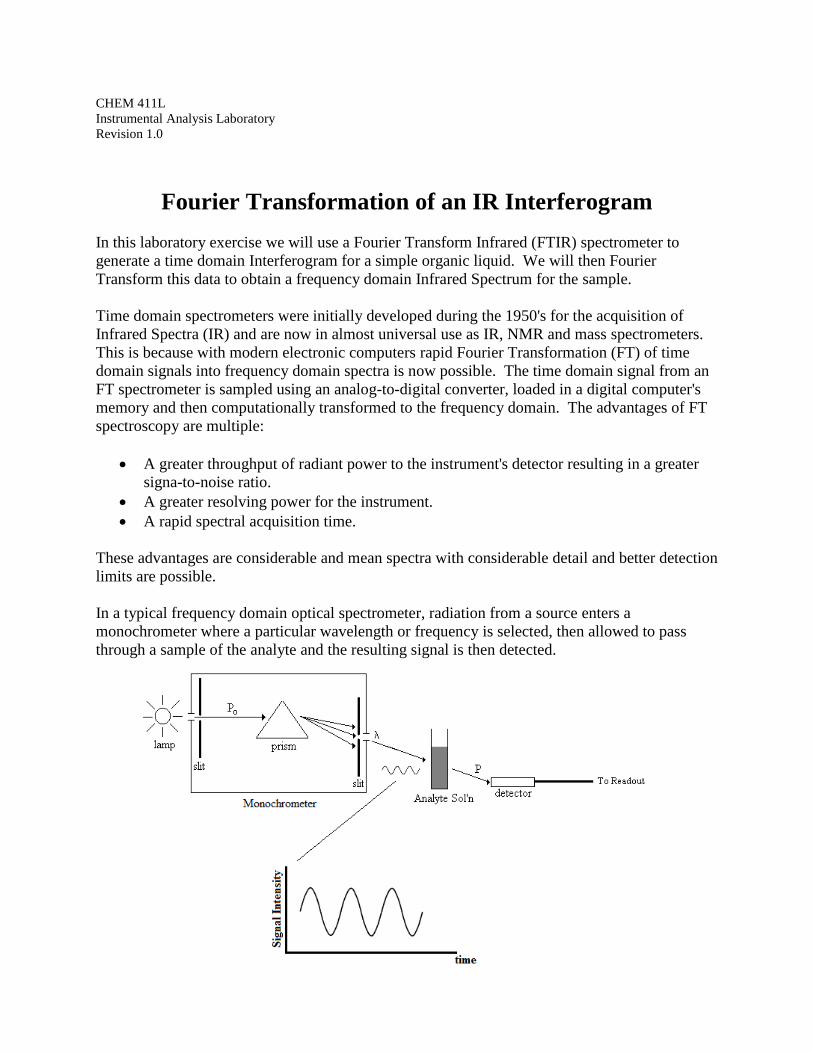
Fourier Transformation of an IR Interferogram

In this laboratory exercise we will use a Fourier Transform Infrared (FTIR) spectrometer to

generate a time domain Interferogram for a simple organic liquid. We will then Fourier

Transform this data to obtain a frequency domain Infrared Spectrum for the sample.

Time domain spectrometers were initially developed during the 1950's for the acquisition of

Infrared Spectra (IR) and are now in almost universal use as IR, NMR and mass spectrometers.

This is because with modern electronic computers rapid Fourier Transformation (FT) of time

domain signals into frequency domain spectra is now possible. The time domain signal from an

FT spectrometer is sampled using an analog-to-digital converter, loaded in a digital computer's

memory and then computationally transformed to the frequency domain. The advantages of FT

spectroscopy are multiple:

A greater throughput of radiant power to the instrument's detector resulting in a greater

signa-to-noise ratio.

A greater resolving power for the instrument.

A rapid spectral acquisition time.

These advantages are considerable and mean spectra with considerable detail and better detection

limits are possible.

In a typical frequency domain optical spectrometer, radiation from a source enters a

monochrometer where a particular wavelength or frequency is selected, then allowed to pass

through a sample of the analyte and the resulting signal is then detected.

P a g e | 2

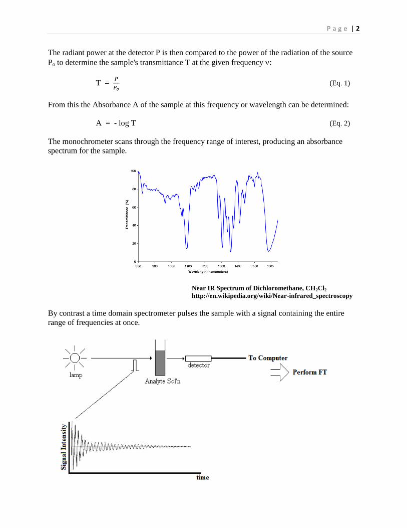
The radiant power at the detector P is then compared to the power of the radiation of the source

Po to determine the sample's transmittance T at the given frequency :

T =

(Eq. 1)

From this the Absorbance A of the sample at this frequency or wavelength can be determined:

A = - log T (Eq. 2)

The monochrometer scans through the frequency range of interest, producing an absorbance

spectrum for the sample.

Near IR Spectrum of Dichloromethane, CH2Cl2

http://en.wikipedia.org/wiki/Near-infrared_spectroscopy

By contrast a time domain spectrometer pulses the sample with a signal containing the entire

range of frequencies at once.

P a g e | 3

After the signal passes through the sample, it is detected and transformed such that it can input

into a digital computer and then Fourier Transformed to yield our usual frequency domain

spectrum.

The Fourier Transform G(f) of a time domain signal g(t) is determined according to:

G(f) =

(Eq. 3)

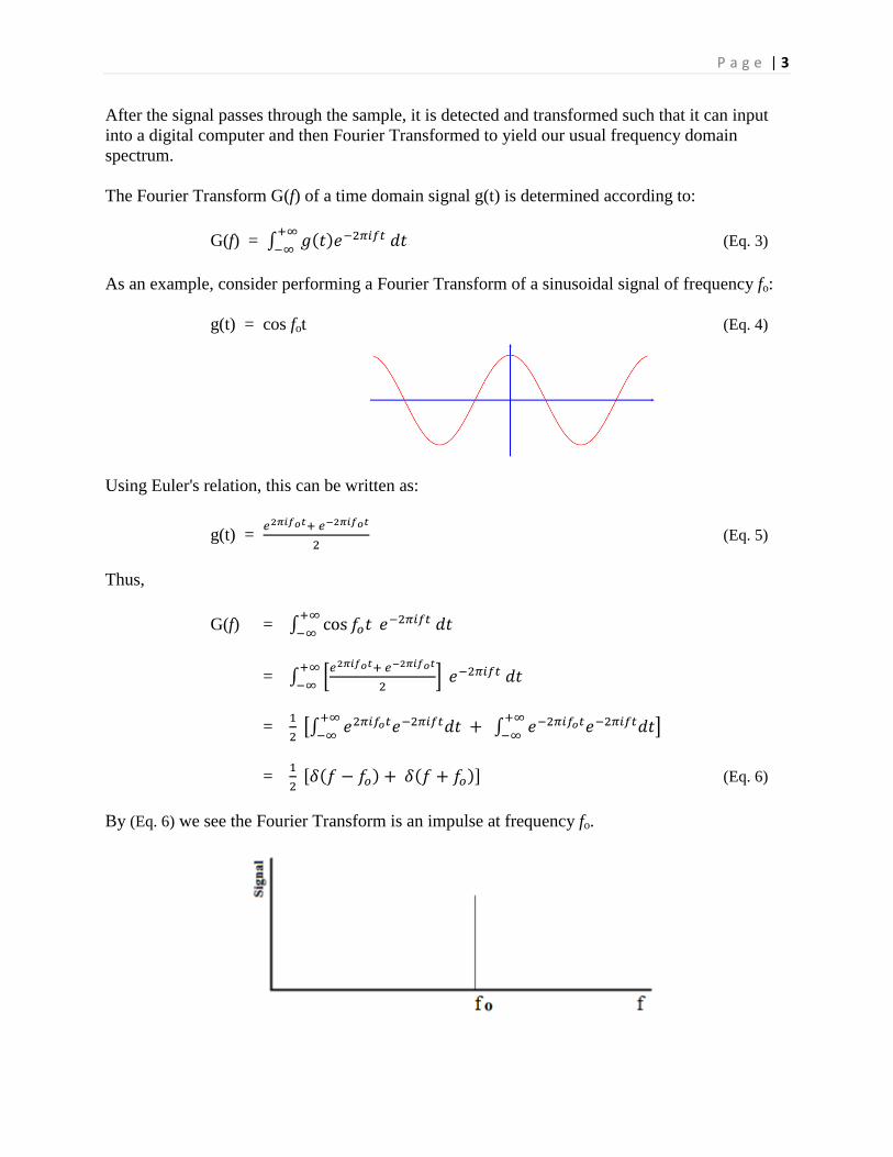
As an example, consider performing a Fourier Transform of a sinusoidal signal of frequency fo:

g(t) = cos fot (Eq. 4)

Using Euler's relation, this can be written as:

g(t) =

(Eq. 5)

Thus,

G(f) =

=

=

=

(Eq. 6)

By (Eq. 6) we see the Fourier Transform is an impulse at frequency fo.

P a g e | 4

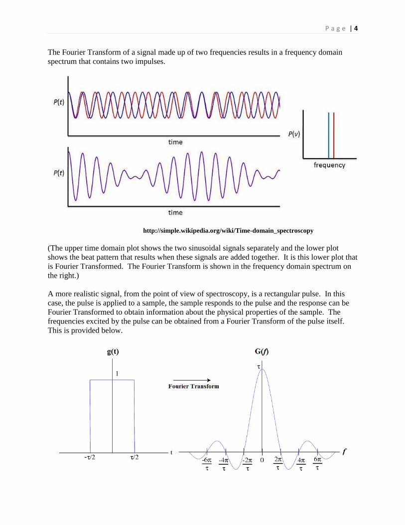
The Fourier Transform of a signal made up of two frequencies results in a frequency domain

spectrum that contains two impulses.

http://simple.wikipedia.org/wiki/Time-domain_spectroscopy

(The upper time domain plot shows the two sinusoidal signals separately and the lower plot

shows the beat pattern that results when these signals are added together. It is this lower plot that

is Fourier Transformed. The Fourier Transform is shown in the frequency domain spectrum on

the right.)

A more realistic signal, from the point of view of spectroscopy, is a rectangular pulse. In this

case, the pulse is applied to a sample, the sample responds to the pulse and the response can be

Fourier Transformed to obtain information about the physical properties of the sample. The

frequencies excited by the pulse can be obtained from a Fourier Transform of the pulse itself.

This is provided below.

P a g e | 5

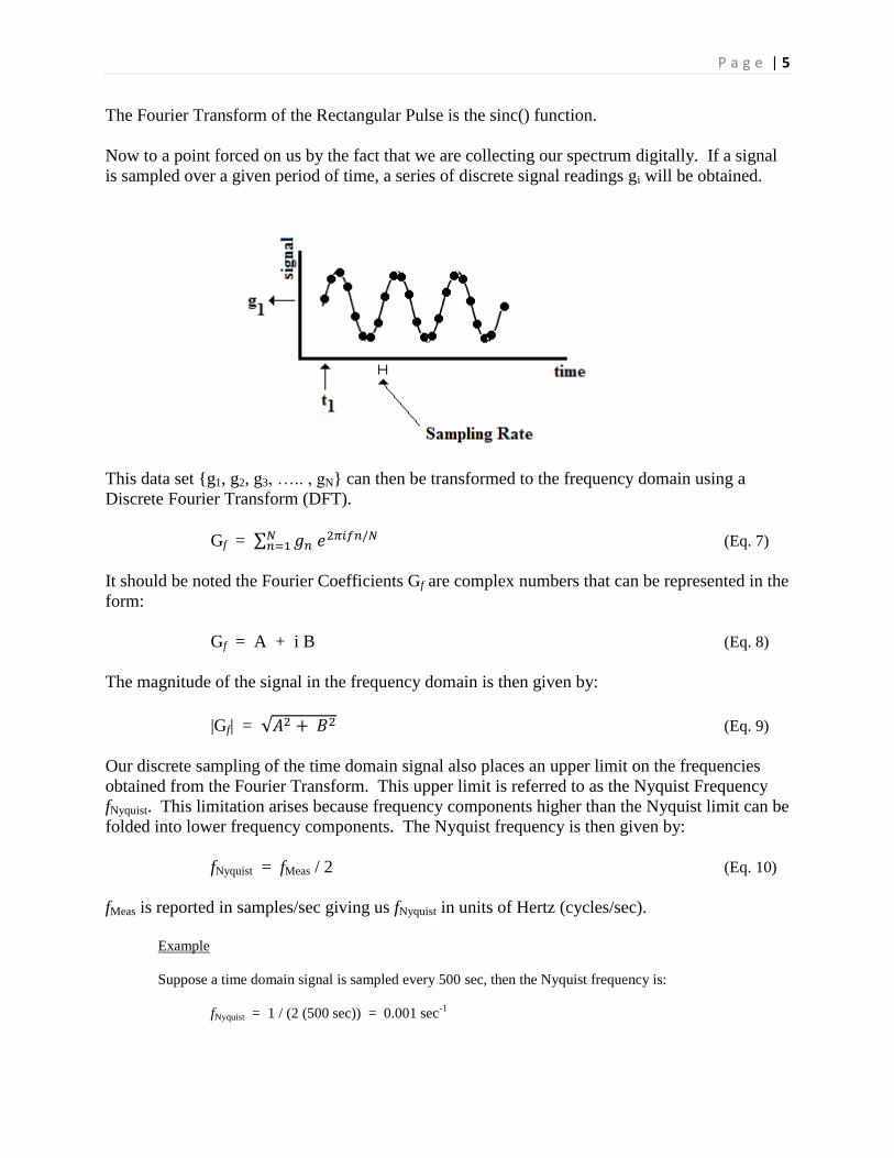
The Fourier Transform of the Rectangular Pulse is the sinc() function.

Now to a point forced on us by the fact that we are collecting our spectrum digitally. If a signal

is sampled over a given period of time, a series of discrete signal readings gi will be obtained.

This data set {g1, g2, g3, ….. , gN} can then be transformed to the frequency domain using a

Discrete Fourier Transform (DFT).

Gf =

(Eq. 7)

It should be noted the Fourier Coefficients Gf are complex numbers that can be represented in the

form:

Gf = A + i B (Eq. 8)

The magnitude of the signal in the frequency domain is then given by:

|Gf| = (Eq. 9)

Our discrete sampling of the time domain signal also places an upper limit on the frequencies

obtained from the Fourier Transform. This upper limit is referred to as the Nyquist Frequency

fNyquist. This limitation arises because frequency components higher than the Nyquist limit can be

folded into lower frequency components. The Nyquist frequency is then given by:

fNyquist = fMeas / 2 (Eq. 10)

fMeas is reported in samples/sec giving us fNyquist in units of Hertz (cycles/sec).

Example

Suppose a time domain signal is sampled every 500 sec, then the Nyquist frequency is:

fNyquist = 1 / (2 (500 sec)) = 0.001 sec-1

P a g e | 6

Calculation of the spectrum using a DFT as prescribed according to equation 7 is

computationally intensive. Note that the calculation of Gf for a single frequency f requires a full

pass through all N data points. If we wish to calculate the spectrum at roughly N different

frequencies, we need to pass through the data set N x N times; meaning the algorithm requires a

computational time proportional to N2. Many of these calculations are redundant. A Fast

Fourier Transform (FFT) algorithm can perform the same calculation at a much reduced

computational cost. FFT's employing a divide-and-conquer strategy reduce the maximum

computational effort to one requiring N log N calculations.

An analysis of FFT algorithms can be found in the Kincaid and Cormen texts of the references.

An implementation of the FFT routine of N.M. Brenner using FORTRAN 77 can be found in the

"Numerical Recipes in Fortran 77" text of the references.

Finally, we turn to a consideration of FT Infrared spectroscopy in particular.

Unfortunately, FTIR spectrometers are not able to employ the simple scheme outlined above to

obtain time domain spectra. This is because of limitations on the response time of the

transducers used to detect an IR signal. Skoog explains:

Time-domain signals, such as those shown [above] cannot be acquired experimentally with

radiation in the frequency range that is associated with optical spectroscopy (1012

to 1015

Hz)

because there are no transducers that will respond to radiant power variations at these high

frequencies. Thus, a typical transducer yields a signal that corresponds to the average power of a

high-frequency signal and not to its periodic variation. To obtain time-domain signals requires,

therefore, a method of converting (or modulating) a high-frequency signal to one of measurable

frequency without distorting the time relationships carried in the signal; that is, the frequencies in

the modulated signal must be directly proportional to those in the original.

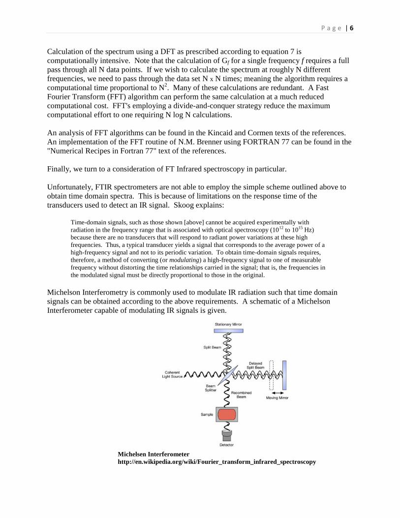
Michelson Interferometry is commonly used to modulate IR radiation such that time domain

signals can be obtained according to the above requirements. A schematic of a Michelson

Interferometer capable of modulating IR signals is given.

Michelsen Interferometer

http://en.wikipedia.org/wiki/Fourier_transform_infrared_spectroscopy

P a g e | 7

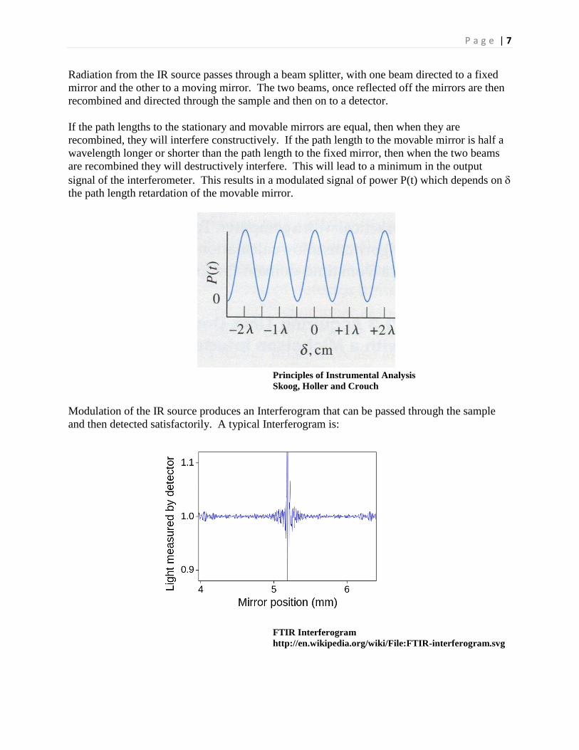
Radiation from the IR source passes through a beam splitter, with one beam directed to a fixed

mirror and the other to a moving mirror. The two beams, once reflected off the mirrors are then

recombined and directed through the sample and then on to a detector.

If the path lengths to the stationary and movable mirrors are equal, then when they are

recombined, they will interfere constructively. If the path length to the movable mirror is half a

wavelength longer or shorter than the path length to the fixed mirror, then when the two beams

are recombined they will destructively interfere. This will lead to a minimum in the output

signal of the interferometer. This results in a modulated signal of power P(t) which depends on

the path length retardation of the movable mirror.

Principles of Instrumental Analysis

Skoog, Holler and Crouch

Modulation of the IR source produces an Interferogram that can be passed through the sample

and then detected satisfactorily. A typical Interferogram is:

FTIR Interferogram

http://en.wikipedia.org/wiki/File:FTIR-interferogram.svg

P a g e | 8

The central peak in the interferogram is at Zero Path Difference (ZPD) and represents a mirror

position giving maximum radiant output power.

In modern FTIR spectrometers, this modulated signal is passed through the sample and is then

measured by a detector. Herres and Gronholz note "…the wings of the interferogram, which

contain most of the useful spectral information, have a very low amplitude. This illustrates the

need for ADC's of high dynamic range in FT-IR measurements. Typically, FT-IR spectrometers

are equipped with 15- or 16-bit ADC's."

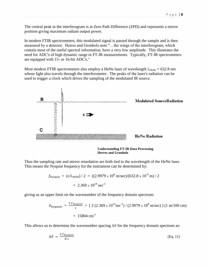
Most modern FTIR spectrometers also employ a HeNe laser of wavelength HeNe = 632.8 nm

whose light also travels through the interferometer. The peaks of the laser's radiation can be

used to trigger a clock which drives the sampling of the modulated IR source.

Understanding FT-IR Data Processing

Herres and Gronholz

Thus the sampling rate and mirror retardation are both tied to the wavelength of the HeNe laser.

This means the Nyquist frequency for the instrument can be determined by:

fNyuquist = (c/HeNe) / 2 = ((2.9979 x 108 m/sec)/(632.8 x 10

-9 m) / 2

= 2.369 x 1014

sec-1

giving us an upper limit on the wavenumber of the frequency domain spectrum:

=

= [ 2 (2.369 x 10

14sec

-1) / (2.9979 x 10

8 m/sec) ] (1 m/100 cm)

= 15804 cm-1

This allows us to determine the wavenumber spacing for the frequency domain spectrum as:

(Eq. 11)

P a g e | 9

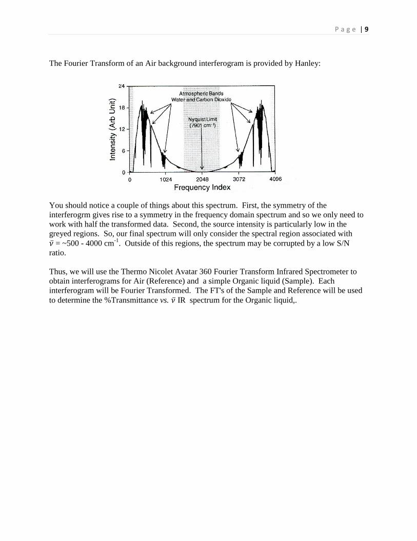
The Fourier Transform of an Air background interferogram is provided by Hanley:

You should notice a couple of things about this spectrum. First, the symmetry of the

interferogrm gives rise to a symmetry in the frequency domain spectrum and so we only need to

work with half the transformed data. Second, the source intensity is particularly low in the

greyed regions. So, our final spectrum will only consider the spectral region associated with

= ~500 - 4000 cm-1

. Outside of this regions, the spectrum may be corrupted by a low S/N

ratio.

Thus, we will use the Thermo Nicolet Avatar 360 Fourier Transform Infrared Spectrometer to

obtain interferograms for Air (Reference) and a simple Organic liquid (Sample). Each

interferogram will be Fourier Transformed. The FT's of the Sample and Reference will be used

to determine the %Transmittance vs. IR spectrum for the Organic liquid,.

P a g e | 10

Procedure

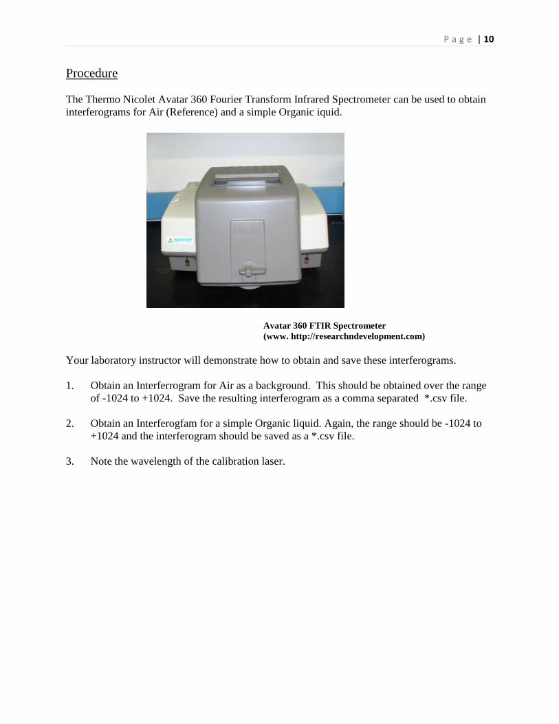
The Thermo Nicolet Avatar 360 Fourier Transform Infrared Spectrometer can be used to obtain

interferograms for Air (Reference) and a simple Organic iquid.

Avatar 360 FTIR Spectrometer

(www. http://researchndevelopment.com)

Your laboratory instructor will demonstrate how to obtain and save these interferograms.

1. Obtain an Interferrogram for Air as a background. This should be obtained over the range

of -1024 to +1024. Save the resulting interferogram as a comma separated *.csv file.

2. Obtain an Interferogfam for a simple Organic liquid. Again, the range should be -1024 to

+1024 and the interferogram should be saved as a *.csv file.

3. Note the wavelength of the calibration laser.

P a g e | 11

Data Analysis

1. Import both Interferograms into an Excel spreadsheet. (To import the *.csv data into Excel,

use the "Open File" dialog and use the "All Files *.*" option in the file type menu.)

2. Excel has a built in FFT feature. This feature can be found under the "Data" tab in the

"Data Analysis" box. Selecting Fourier Transform will open a dialog box that will allow

for the input of the data ranges containing the Iterferogram data and the FFT output. (This

feature must be "installed" as it is usually not part of the default configuration for Excel.)

It should be noted that Excel's FFT algorithm requires a data set of 2N data points. Your

data set will range from -1024 to +1024 and so will have 211

+ 1 data points because of the

"0". Simply select a data range for input into the FFT routine that has one less data points

than the full data set.

Fourier Transform both your Reference and Sample Interferograms. The output will be as

complex numbers.

3. Use Excel's IMABS() function to calculate the magnitude of the complex output. This

gives you data for Io (Reference) and I (Sample).

4. Use your Io and I data to determine the %T for you sample.

5. Calibrate the wavenumbers for each spectral data point using your knowledge of the

Nyquist frequency for the instrument.

6. Prepare a %T vs. for your organic sample. Remember, you should truncate this spectrum

to ~500 - 4000 cm-1

. It is customary to present the spectrum as ranging from 4000 cm-1

to

500 cm-1

; reversing the wavenumber axis.

You should submit a Memo Style report of the above findings. Be sure to include both

Interferograms, Fourier Transformed data for both samples and the final spectrum. What

is "Zero Padding" and how would this help improve your spectrum?

P a g e | 12

References

Cormen, Thomas H., Leiserson, Charles E. and Rivest, Ronald L. (1998) "Introduction to

Algorithms" The MIT Press, Cambridge, Massachusetts.

Introduction to FT-IR Spectroscopy. (2013) Retrieved September 26, 2013,

http://assets.newport.com/webDocuments-EN/images/FTIR_Spectroscopy.PDF

Herres, Werner and Gronholz, Joern; Understanding FT-IR Data Processing. (2013) Retrieved

September 26, 2013, http://www.lightsource.ca/files/download.php?id=2677&view=1

Kincaid, David and Cheney, Ward (2002) "Numerical Analysis: Mathematics of Scientific

Computing, 3rd

Ed." Brooks/Cole, Pacific Grove, California.

The Power of the Fourier Transform for Spectroscopists. (2013) Retrieved September 26, 2013,

from http://chemwiki.ucdavis.edu/Physical_Chemistry/Spectroscopy/Fundamentals/

The_Power_of_the_Fourier_Transform_for_Spectroscopists

Press, William H., Teukolsky, Saul A., Vetterling, William T. and Flannery, Brian P. (1986)

"Numerical Recipes in Fortran 77: The Art of Scientific Computing, 2nd

Ed." Cambridge

University Press, New York.

Skoog, Douglas A., Holler, F. James and Crouch, Stanley R. (2007) " Principles of Instrumental

Analysis, 6th

Ed." Thomson, Belmont, California.