Fractal Analysis of Cardiac

Dynamics: The Application of

Detrended Fluctuation Analysis

on Short-term Heart Rate

Variability

Pandelis Perakakis

Personality, Evaluation and Psychological Treatment

Granada University

A thesis submitted for the degree of

PhilosophiæDoctor (PhD)

2009 October

Editor: Editorial de la Universidad de GranadaAutor: Pandelis PerakakisD.L.: Gr. 156-2010ISBN: 978-84-692-8392-9

ii

SUPERVISOR REPORT

Dr. Jaime Vila Castellar, professor of psychology at the department of per-

sonality, evaluation and psychological treatment in the university of Granada,

Dr. Gustavo Reyes del Paso, professor of psychology at the department of per-

sonality, evaluation and psychological treatment in the university of Jaen,

Dr. Lourdes Anllo–Vento, professor of psychology at the department of per-

sonality, evaluation and psychological treatment in the university of Granada,

CERTIFY: that this doctoral dissertation entitled Fractal Analysis of Car-

diac Dynamics: The Application of Detrended Fluctuation Analysis

on Short-term Heart Rate Variability, was written by Pandelis Perakakis

under our supervision and fulfills the qualitative criteria required for its defense.

1st of October 2009

Jaime Vila Castellar

Gustavo Reyes del Paso

Lourdes Anllo–Vento

iii

iv

Στην Αγαπη�ένη �ου Γιαγιά

vi

Acknowledgements

The ideas and results presented in this doctoral dissertation represent the

Ithaca of an exciting four-year academic and personal adventure. Unfortu-

nately, there is no space here to describe the marvelous journey that lead

to this thesis. Perhaps, the only thing I can do is to remember a few of the

people that have accompanied and shared with me all the wonderful and

difficult moments.

First of all, I would like to acknowledge the guidance and support of my su-

pervisors Jaime Vila, Gustavo Reyes and Lourdes Anllo-Vento. Especially

Jaime has been a continuous motivation to stay on the academic track, pro-

viding an outstanding example both as a scientist and as a person. He is

the academic father of a wonderful family, the group of human psychophys-

iology in the University of Granada, of which I have been a member for the

last seven years. This thesis was only possible thanks to all of them.

The most interesting aspect of my academic life these past years has been

without doubt the opportunity it gave me to travel and meet exciting cul-

tures and remarkable people. In Madrid, I met my good friend and scientist

Michael Taylor with whom I started discussing about nature’s complexity

during our unforgettable gastronomical orgies at my regular weekend vis-

its. In Rio de Janeiro, “La Ciudad Maravillosa”, I had the opportunity

to meet and collaborate with professors Eliane Volchan, Walter Machado

Pinheiro and all the wonderful and talented people in their research groups.

In Moscow, I was kindly welcomed to the Buetyko clinic by Dr. Andrey

Novozhilov. Finally, in Boston I was warmly received by professor Eugene

Stanley in the Center of Polymer Studies at Boston University, where I

had the pleasure to enjoy interesting conversations with professor Plamen

Ivanov.

On a more personal note I wish to thank Chara Theologidou for being

always next to me in so many different ways throughout the years and

Michael Vousdouka for the “finals” and the innumerable discussions about

“Life, the Universe and Everything”. Along with them comes a long list of

beautiful people around the world with whom I laughed, cried, made love,

played music, travelled and talked for hours with a mind blurred from wine

or stimulated by a hot cup of coffee. They know who they are and I thank

them for the magic.

Last, I wish to dedicate this effort to my family, at my hometown Thessa-

loniki in Greece. Although I have spent all these years away from them, I

always recognize their presence in anything I do or feel. They are who I am

and I owe them everything.

Abstract

Fractal measures of heart rate variability have been proposed as comple-

mentary to time and frequency domain indices and, in many cases, have

proven to be valid predictors of cardiovascular disease. However, their re-

lationship with respiratory parameters and more common health indicators

such as vagal tone is still not clear. In this doctoral dissertation, we examine

the effect of breathing frequency, average heart period and pharmacological

parasympathetic blockade on the fractal properties of short-term cardiac

dynamics. Heart period analysis is performed with a mathematical soft-

ware (KARDIA) developed for the purpose of our studies, which is also

presented in this thesis. The results of our first study revealed that: 1)

the periodical properties of RSA produce a change of the correlation ex-

ponent in HRV at a scale corresponding to the respiratory period, 2) the

short-term DFA exponent is significantly reduced when breathing frequency

rises from 0.1Hz to 0.2Hz. In the second study atropine was administered

to six healthy males in a controlled laboratory setting. Parasympathetic

blockade produced a significant increase in the α1 scaling exponent assessed

by detrended fluctuation analysis. We showed that this was produced by

smooth local trends in the data, rather than an alteration in underlining

dynamics. Our results call attention to a methodological and conceptual

problem related to the application of fractal measures to a limited range of

scales in which single physiological control mechanisms exert a dominant

influence.

x

Contents

List of Figures xv

List of Tables xix

Glossary xxi

1 Introduction 1

2 Heart Rate Variability 5

2.1 Time Domain Measures . . . . . . . . . . . . . . . . . . . . . . . . . . . 5

2.2 Frequency Domain Measures . . . . . . . . . . . . . . . . . . . . . . . . 6

2.3 Nonlinear Measures . . . . . . . . . . . . . . . . . . . . . . . . . . . . . . 7

3 Fractal Variability 11

3.1 Fractals in Space and Time . . . . . . . . . . . . . . . . . . . . . . . . . 11

3.1.1 Geometrical Fractals . . . . . . . . . . . . . . . . . . . . . . . . . 11

3.1.2 Temporal Fractals . . . . . . . . . . . . . . . . . . . . . . . . . . 12

3.2 Fractal Analysis of Cardiac Dynamics . . . . . . . . . . . . . . . . . . . 17

4 KARDIA: a Matlab Software for the Analysis of Cardiac InterbeatIntervals 21

4.1 Introduction . . . . . . . . . . . . . . . . . . . . . . . . . . . . . . . . . . 21

4.2 Program Description . . . . . . . . . . . . . . . . . . . . . . . . . . . . . 22

4.2.1 The graphical user interface . . . . . . . . . . . . . . . . . . . . . 23

4.2.1.1 Load IBI data and event information panel . . . . . . . 24

4.2.1.2 PCR analysis panel . . . . . . . . . . . . . . . . . . . . 24

4.2.1.3 HRV analysis panel . . . . . . . . . . . . . . . . . . . . 25

xi

CONTENTS

4.2.1.4 Results panel . . . . . . . . . . . . . . . . . . . . . . . . 27

4.2.1.5 Toolbar buttons . . . . . . . . . . . . . . . . . . . . . . 28

4.2.2 System requirements . . . . . . . . . . . . . . . . . . . . . . . . . 28

4.2.3 Installation Procedure . . . . . . . . . . . . . . . . . . . . . . . . 29

4.2.4 Availability . . . . . . . . . . . . . . . . . . . . . . . . . . . . . . 29

4.3 Sample runs . . . . . . . . . . . . . . . . . . . . . . . . . . . . . . . . . . 29

4.4 Conclusion . . . . . . . . . . . . . . . . . . . . . . . . . . . . . . . . . . 31

5 Breathing Frequency Bias in Fractal Analysis of Heart Rate Variabil-ity 33

5.1 Introduction . . . . . . . . . . . . . . . . . . . . . . . . . . . . . . . . . . 33

5.1.1 Detrended Fluctuation Analysis . . . . . . . . . . . . . . . . . . . 35

5.1.2 Application to IBI records . . . . . . . . . . . . . . . . . . . . . . 35

5.1.3 Effects of sinusoidal trends on DFA . . . . . . . . . . . . . . . . . 36

5.2 Method . . . . . . . . . . . . . . . . . . . . . . . . . . . . . . . . . . . . 40

5.3 Results . . . . . . . . . . . . . . . . . . . . . . . . . . . . . . . . . . . . . 41

5.4 Discussion . . . . . . . . . . . . . . . . . . . . . . . . . . . . . . . . . . . 42

5.4.1 Re-interepreting results of previous studies . . . . . . . . . . . . 45

5.4.2 General conclusions and suggestions for further research . . . . . 46

6 The Effect of Parasympathetic Blockade on Fractal Analysis of HeartRate Variability 49

6.1 Introduction . . . . . . . . . . . . . . . . . . . . . . . . . . . . . . . . . . 49

6.2 Methods . . . . . . . . . . . . . . . . . . . . . . . . . . . . . . . . . . . . 51

6.2.1 Participants . . . . . . . . . . . . . . . . . . . . . . . . . . . . . . 51

6.2.2 Design . . . . . . . . . . . . . . . . . . . . . . . . . . . . . . . . . 51

6.2.3 Procedure . . . . . . . . . . . . . . . . . . . . . . . . . . . . . . . 52

6.2.4 Data reduction and analysis . . . . . . . . . . . . . . . . . . . . . 52

6.3 Results . . . . . . . . . . . . . . . . . . . . . . . . . . . . . . . . . . . . . 53

6.4 Discussion . . . . . . . . . . . . . . . . . . . . . . . . . . . . . . . . . . . 57

6.5 Conclusion . . . . . . . . . . . . . . . . . . . . . . . . . . . . . . . . . . 60

7 Discussion 61

Bibliography 67

xii

CONTENTS

Annex I 73

Annex II 77

xiii

CONTENTS

xiv

List of Figures

3.1 The Mandelbrot set. A mathematical fractal defined as a set of points in

the complex plane resulting by the iteration of the quadratic polynomial

zn+1 = z2n + c . . . . . . . . . . . . . . . . . . . . . . . . . . . . . . . . . 12

3.2 Schematic representations of self-similar structures and self-similar fluc-

tuations. The tree-like, spatial fractal (Left) has self-similar branchings,

such that the small-scale structure resembles the large-scale form. A

fractal temporal process, such as healthy heart rate regulation (Right),

may generate fluctuations at different time scales that are statistically

self-similar . . . . . . . . . . . . . . . . . . . . . . . . . . . . . . . . . . . 13

3.3 Types of noise. Three examples of signals h(t) plotted as functions of

time t: white noise (A), 1/f - or “pink” noise (B) and Brownian noise

(C) (1) . . . . . . . . . . . . . . . . . . . . . . . . . . . . . . . . . . . . . 14

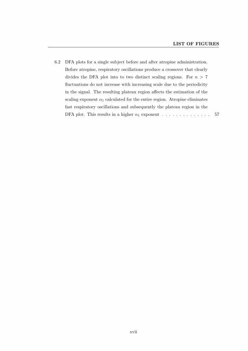
3.4 Power spectra of distinct types of noise. White noise (A), 1/f noise (B)

and Brownian noise. The lines fitted to the spectra have slopes of 0.01,

−1.31 and −1.9, respectively (1) . . . . . . . . . . . . . . . . . . . . . . 16

3.5 Comparing heart rate patterns. Recordings A and C are from patients in

sinus rhythm with severe congestive heart failure and D is from a subject

with atrial fibrillation, which produces an erratic heart rate. Recording

B exhibits fractal variability (2) . . . . . . . . . . . . . . . . . . . . . . . 18

4.1 The graphical user interface of KARDIA . . . . . . . . . . . . . . . . . . 23

4.2 The PCR results panel. The grand average over all subjects indicates a

potentiated bradycardia in the unpleasant picture condition (blue line)

compared to control (green line) . . . . . . . . . . . . . . . . . . . . . . 30

xv

LIST OF FIGURES

4.3 The HRV results panel. Figure 4.3(a) shows the spectral graph of a 5

min segment before atropine administration. In Figure 4.3(b), which

presents a spectral graph for the same subject after atropine administra-

tion, we observe the elimination of respiratory-related oscillations due to

parasympathetic blockade . . . . . . . . . . . . . . . . . . . . . . . . . . 31

5.1 Plot of log F (n) vs. log n from a healthy subject (circles) and from a sub-

ject with congestive heart failure (triangles). Arrows indicate crossovers

that divide the DFA plot into two distinct scaling regions . . . . . . . . 37

5.2 Crossover behavior of the fluctuation function F (n) for correlated noise

superimposed with a sinusoidal function with period T = 15. The fluc-

tuation function for noise and the fluctuation function for the sinusoidal

trend are shown separately for comparison. The arrow indicates the scal-

ing crossover at scale nx = 15 (log10(15) = 1.1761) corresponding to the

period of the sinusoidal trend . . . . . . . . . . . . . . . . . . . . . . . . 39

5.3 Crossover behavior of the F(n) function at different respiratory frequen-

cies in one subject. Changes in scaling exponents indicate the location

of the crossover. The crossover occurs at smaller scales as breathing

becomes more rapid . . . . . . . . . . . . . . . . . . . . . . . . . . . . . 43

5.4 Crossover behavior of the F(n) function in three subjects (A, B and C)

during spontaneous breathing. In the top row we observe a broad-band

RSA at progressively faster frequencies as we move from subject A to

subject C. Arrows on the DFA plots in the second row indicate scaling

crossovers that are encountered at smaller scales for faster breathing

frequencies . . . . . . . . . . . . . . . . . . . . . . . . . . . . . . . . . . 44

6.1 IBI series and power spectrum graphs for a single subject. IBI series

illustrate a short 50-sec segment obtained from the entire 5-min record.

The number of heartbeats in the two short segments indicates a heart

rate increase in the atropine condition. The spectral graphs clearly show

the elimination of fast respiratory oscillations just below 0.2 Hz after

atropine administration. Note the difference in the scale of the figures

before and after atropine . . . . . . . . . . . . . . . . . . . . . . . . . . . 55

xvi

LIST OF FIGURES

6.2 DFA plots for a single subject before and after atropine administration.

Before atropine, respiratory oscillations produce a crossover that clearly

divides the DFA plot into to two distinct scaling regions. For n > 7

fluctuations do not increase with increasing scale due to the periodicity

in the signal. The resulting plateau region affects the estimation of the

scaling exponent α1 calculated for the entire region. Atropine eliminates

fast respiratory oscillations and subsequently the plateau region in the

DFA plot. This results in a higher α1 exponent . . . . . . . . . . . . . . 57

xvii

LIST OF FIGURES

xviii

List of Tables

5.1 Results for 14 subjects breathing at frequencies of 0.1, 0.2, and 0.25 Hz.

IBI is the average cardiac interbeat interval, nx is the predicted scale

of the respiratory crossover, α1 and α2 are the exponents for the two

scaling regions defined by the crossover, and α4−16 is the exponent for

the region from 4 to 16 beats. There are data gaps at 0.25 Hz due to

the small value of nx in the fast breathing condition. . . . . . . . . . . . 42

6.1 Interbeat intervals (IBI), high-frequency HRV (HF), low-frequency HRV

(LF), and short-term HRV DFA scaling exponent (α1) before and after

administration of atropine or placebo. Standard deviations are given in

parentheses. . . . . . . . . . . . . . . . . . . . . . . . . . . . . . . . . . . 54

xix

GLOSSARY

xx

Glossary

α scaling exponent obtained by DFA

α1 short-term scaling exponent usually

calculated for the range between 4

and 16 heartbeats

α2 long-term scaling exponent usually

calculated for the range between 17

and 64 (or more) heartbeats

1/f noise also pink noise; a signal or pro-

cess with a frequency spectrum such

that the power spectral density is in-

versely proportional to the frequency

ANS Autonomous nervous system

DFA Detrended Fluctuation Analysis; al-

gorithm used to quantify long-term

correlations in nonstationary time se-

ries

DFT Discrete Fourier transform

ECG Electrocardiogram

ERP Event-related Potentials

Fractal a rough or fragmented geometric

shape that can be split into parts,

each of which is (at least approxi-

mately) a reduced-size copy of the

whole

HF High frequency spectral power

hr hours

HRV Heart rate variability; the variation

in the period between heartbeats

that is measured as an index of auto-

nomic control on the heart

IBI Interbeat interval

LF Low frequency spectral power

min minutes

ms milliseconds

N Normal heartbeat as opposed to ec-

topic beats or other artifacts

NN Time interval between normal heart-

beats

NN50 Absolute count of differences be-

tween successive NN intervals greater

than 50 ms

PCR Phasic cardiac responses

pNN50 Proportion of differences between

successive NN intervals greater than

50 ms

RMS Root mean square

RMSSD Root mean square of successive dif-

ferences

RSA Respiratory sinus arrhythmia; a nat-

urally occurring variation in heart

rate that occurs during a breathing

cycle

Scale invariance also Self-similarity; property

of objects (geometrical shapes or

fluctuating time series) that do not

change if length scales (or energy

scales) are multiplied by a common

factor

Scaling crossover Change in scaling proper-

ties of HRV correlations usually due

to persistent trends in the data

SDANN Standard deviation of sequential 5

min heartbeat interval means

SDNN Standard deviation of heartbeat in-

tervals

SOC Self-organized criticality; theory pro-

posed to explain why certain physical

and biological systems exhibit long-

range power-law correlations

xxi

GLOSSARY

ULF Ultra low frequency spectral power VLF Very low frequency spectral power

xxii

Chapter 1

Introduction

The variability in the heart rate signal (Heart Rate Variability; HRV) is extensively

being studied as an indirect index of autonomic regulation. In psychophysiological

experiments, measures of HRV in resting states are used to elucidate the relationship

between autonomic state and cognitive performance or emotional responses. Moreover,

HRV indices have repeatedly proven useful in distinguishing cardiovascular patients

from healthy populations. Despite their ample use in diverse fields, there are clear

methodological problems associated with the estimation and interpretation of HRV

measures. Available HRV metrics are continuously being refined and new techniques

introduced. In recent years, the study of HRV has attracted the interest of statistical

physicists who observed a resemblance of HRV fluctuations to complex signals deriving

from physical systems characterized by nonlinear dynamics.

This discovery of nonlinearities in HRV triggered a series of studies with remark-

able results. Various investigations confirmed that long-term HRV fluctuations are not

random, but exhibit long-term correlations that do not exhibit any characteristic scale,

but are rather “scale invariant”. This type of scale invariant variability is also known

as fractal and the methodology employed to evaluate it is often called fractal analy-

sis. It was discovered that the fractal organization of HRV fluctuations is distorted in

cardiovascular patients and elderly populations. One of the most popular algorithms

applied to HRV signals in order to reveal these complex fractal fluctuation patterns is

the Detrended Fluctuation Analysis (DFA). DFA was introduced in 1995 and has been

used since then in more than 700 HRV studies.

1

1. INTRODUCTION

One of the interesting findings resulting from the application of DFA to human HRV,

was the clear distinction between the characteristics of long and short-term HRV fluc-

tuation patterns. While long-term HRV shows similarities to critical physical systems,

short-term HRV fluctuations are characterized by strong correlations that indicate a

different organization of the underlining control mechanisms. It was hypothesized that

strong correlation patterns in short-term HRV are due to the smooth heart rate oscilla-

tions associated with breathing, a phenomenon known as Respiratory Sinus Arrhythmia

(RSA). Nevertheless, no experimental study properly addressed this hypothesis. On

the contrary, all published investigations reporting results on short-term DFA, attribute

their findings in the underlining organization of cardiac dynamics, without considering

RSA in their interpretations. Therefore, despite the important number of publications

examining short-term DFA exponents, the physiologic significance of this index remains

elusive.

In this dissertation we experimentally tested the hypothesis that short-term DFA

exponents are sensitive to RSA and therefore to breathing parameters. The findings

in our first study, confirmed this hypothesis and clarified the physiological significance

of this new HRV measure. In a second experiment, we tested our interpretation by

comparing subjects with impaired autonomic control induced by drug administration,

and control individuals. The results re-confirmed our hypotheses and further supported

the mathematical and physiological interpretation of the effects of RSA and generally

smooth systematic trends on the application of fractal measures to short-term HRV.

The conclusions drawn from our studies question the interpretation of results ob-

tained by the application of DFA to short-term HRV, based on underlining fractal

properties. On the contrary, we assert that DFA can be used to assess the fractal

properties of long-term HRV. We discuss the potential benefits of this line of research

for our theoretical understanding of physiologic control and for the clinical diagnosis

of cardiovascular disorders. In terms of theoretical understanding, fractal physiology

questions the paradigm of homeostasis that has been central to physiology in the last

century and which postulates that physiological systems normally operate to reduce

variability and maintain a constancy of internal function. Instead, fractal physiology

suggests that internal feedback mechanisms produce a complex variability that renders

the system more flexible and adaptive to external perturbations. In terms of clinical

diagnosis, small deviations from fractal organization in cardiac dynamics could prove a

2

sensitive index of impaired autonomic regulation, long before the actual cardiovascular

disorder manifests with clear symptoms.

We begin this thesis with a theoretical introduction of related concepts. In the

second chapter we introduce the concept of HRV and review some of the most common

measures. The third chapter presents the concept of fractal analysis applied to tempo-

ral processes. What follows are three articles that were submitted to highly-esteemed

academic journals. The fourth chapter presents KARDIA, a software program devel-

oped for the analysis of cardiac data used in this dissertation. This paper was accepted

for publication by the journal Computer Methods and Programs in Biomedicine. The

fifth chapter introduces the details of the Detrended Fluctuation Analysis algorithm

and describes our first study exposing the breathing frequency bias in the fractal anal-

ysis of short-term HRV. This article was published in Biological Psychology (vol.82,

pp.82–88). The sixth chapter is a presentation of our second study on the effects of

parasympathetic blockade on DFA, which further supports the findings and interpre-

tation of the first study. This paper was submitted to the Journal of Cardiovascular

Electrophysiology. We conclude with a discussion of our results and their implications

for future research.

3

1. INTRODUCTION

4

Chapter 2

Heart Rate Variability

In healthy individuals heart rate is neither constant nor periodic. Instead, the variabil-

ity in heart rate fluctuations is determined by the complex dynamics of the sympathetic

and the parasympathetic branches of the autonomic nervous system (ANS), which inter-

act at the impulse generating tissue located in the right atrium of the heart (sinoatrial

node). Generally, sympathetic stimulation increases heart rate, while parasympathetic

stimulation decreases it. Heart rate variability is a composite of numerous influences

reflecting physiological regulatory mechanisms. In the recent past there has been a

spurt of research efforts involving HRV, based on the conviction that disentangling

the sources of variation in cardiac dynamics will provide valuable information on the

cardiovascular autonomic regulation of the heart.

2.1 Time Domain Measures

In time domain analysis of HRV the intervals between successive normal R waves in the

electrocardiogram are measured over the period of recording (3). A variety of statistical

metrics can be calculated from the intervals directly and others can be derived from

the differences between intervals. The square root of variance (SDNN) is probably the

most popular time domain measurement of HRV. A significant part of the variance of

this measurement (30-40%) is attributed to day-night differences in the NN intervals (N

stands for normal heartbeat as opposed to ectopic beats or other artifacts). Therefore,

long ECG recordings (at least 18-hr) are required for its correct estimation (3). The

standard deviation of the 5-min average NN intervals (SDANN) is another version of

5

2. HEART RATE VARIABILITY

the same measurement, although it is much smoother and less sensitive to unedited

artifacts, missed beats and ectopic complexity (4). Both of these parameters are more

sensible to slow trends in the heart rate data and are therefore used to quantify long-

term fluctuations.

The square root of the mean squared differences of successive NN intervals (RMSSD),

the absolute count of differences between successive NN intervals greater than 50 ms

(NN50), and the proportion of differences greater than 50 ms (pNN50), are the most

common variables calculated as differences between normal R-R intervals. In general,

time domain measures derived from the differences between successive heartbeats have

shown to correlate well with vagal activity and are mostly used to quantify parasympa-

thetic modulation of cardiac dynamics (5). RMSSD is a metric that is sensitive to fast

frequency heart rate fluctuations (6). It correlates significantly with frequency domain

measures of HRV that quantify the power of rapid oscillations in the heart rate signal.

Pharmacological blockade studies further indicate that the RMSSD statistic is sensitive

to vagal cardiac control, and it has even been suggested to be superior to spectral meth-

ods as it may be less sensitive to variations in respiratory patterns (7). This notion,

however, has been criticized in a recent study which revealed that the RMSSD statistic

is biased by basal heart period and that between-subjects correlations of absolute lev-

els of RMSSD and high frequency spectral variability were higher than within-subjects

changes in these measures (6).

2.2 Frequency Domain Measures

Time domain indices of HRV provide statistical information on total variability over

a period of time, without resolving it further. Frequency domain indices on the other

hand provide information on the distribution of HRV power as a function of frequency.

Power spectral analysis of short segments (usually around 5 min) of beat-to-beat HRV,

either based on fast Fourier transformation or on autoregression techniques, is probably

the most common frequency domain measure. This type of short-segment analysis

usually reveals three peaks in distinct bands in the power spectra. The high frequency

(HF) band (0.15 to 0.4 Hz) reflects respiratory modulation via efferent impulses on

the cardiac vagus nerves and is abolished by parasympathetic blockade (8). It has

been shown that when breathing frequency changes, the center frequency of the HF

6

2.3 Nonlinear Measures

peak is displaced according to the respiratory rate. In addition, HF variability is

also completely abolished during breath holding tasks (9). The low frequency (LF)

spectral band (0.04 to 0.15 Hz) is modulated by baroreflexes with a combination of

sympathetic and parasympathetic efferent nerve traffic to the sinoatrial node (10; 11;

12; 13; 14; 15). Standing or head up tilt causes a modest increase in LF power and a

substantial decrease in HF power (14). Atropine almost abolishes the LF peak, and beta

blockade prevents the increase caused by standing up. Various manipulations of HF

and LF power or the use of LF/HF ratio have been pursued in an attempt to estimate

sympathetic activity. These manipulations are based in a simplistic understanding

of autonomic interactions and in most cases have not led to satisfying results (3).

Finally, the mechanism responsible for the very low frequency (VLF) spectral band (0

to 0.04 Hz) is a matter of dispute. VLF power is also abolished by atropine, suggesting

that it uses a parasympathetic efferent limp (15). It has also been suggested that

the VLF power reflects the activity partly of the renin-aldosterone system and partly

thermoregulation or vasomotor activity (16).

The spectral analysis of 24-hr heart rate recordings reveals information about much

slower oscillations than those observed in a 5-min recording. The lowest frequency band

in the 24-hr power spectrum is the ultra low frequency (ULF) band (0 to 0.003 Hz),

which quantifies fluctuations in R-R intervals with periods between 5 min and 24 hrs.

The physiological basis for these slow oscillations in the heart rate is less clear. ULF

indices, however, have proven to be powerful risk predictors in cardiovascular diseases

(17).

2.3 Nonlinear Measures

Time and frequency domain measures of HRV quantify the variability of heart rate

fluctuation in characteristic time scales. Nonlinear measures on the contrary attempt

to quantify the structure or complexity of the R-R interval time series. A common linear

measure, for example, would not be able to distinguish between a random, a periodic

and a normal series of R-R intervals if all three had the same standard deviation.

These three types of signals, however, have a totally different underlying organization,

which may be more informative about autonomic regulation than the variation in an

individual frequency band (3).

7

2. HEART RATE VARIABILITY

The interest in the nonlinear analysis of HRV was motivated by the demonstration

of nonlinearities in the R-R interval time series, resulting by the complex interactions

and the numerous feedback loops that ultimately determine the sympathetic and vagal

cardiac outflow. According to many researchers, the extraordinary complexity, non-

linearity and nonstationarity generated by living organisms and present in the cardiac

dynamics, as well as in many other physiological systems, defy traditional mechanis-

tic approaches based on homeostasis and conventional bio-statistical methodologies

(2; 18; 19; 20; 21; 22). It is already a widespread belief that physiological time series

contain more information than can be assessed by common statistical indices and that

applying concepts from statistical physics and complexity science to a wide range of

biomedical problems, from molecular to organismic levels, may provide us with impor-

tant insights on how physiological complex systems work (2).

A large number of nonlinear indices of HRV has been studied and new are developed

continuously. Only a few of them, however, have shown a clear clinical utility. One

of them is the power law slope which is obtained by the spectral power measured over

24 hrs. The spectral power will show a progressive exponential increase in amplitude

with decreasing frequency. This is the characteristic 1/f or “pink” noise observed in

complex biological systems which do not exhibit any characteristic scale (scale invariant

or fractal) (1; 23). This relationship can be also plotted as the log of power versus the

log of frequency, which transforms the exponential curve to a line whose slope can be

estimated. In a log-log plot, the power law function between 10−2 Hz and 10−4 Hz is

linear with a negative slope, and reflects the degree to which the structure of the R-R

interval time series is self similar over a scale of minutes to hours (3). Decreased power

law slope is a marker for increased risk of mortality after myocardial infarction (24).

Nonlinear measures of heart rate variability also include the analysis of the Poincare

plots, Lyapunov exponent, fractal dimension, approximate entropy, heart rate turbu-

lence and many others, but these indices have not been that broadly investigated or

correlated with other health measures (25).

Both linear and nonlinear measures of HRV have been used to quantify risk in a

wide variety of both cardiac and noncardiac disorders such as stroke, multiple sclerosis,

end stage renal disease, neonatal distress, diabetes mellitus, ischemic heart disease, my-

ocardial infarction, cardiomyopathy patients awaiting cardiac transplantation, valvular

heart disease, and congestive heart failure. HRV analysis has also been used to assess

8

2.3 Nonlinear Measures

the autonomic effects of drugs, including beta blockers, calcium blockers, psychotropic

agents, antiarrhythmics and cardiac glycosides (3).

9

2. HEART RATE VARIABILITY

10

Chapter 3

Fractal Variability

Contrary to the common notion that physiological systems, including the healthy heart-

beat, are regulated according to the classical principal of homeostasis, operating to re-

duce variability and to achieve an equilibrium-like state, it has been shown that, under

normal conditions, beat-to-beat heart rate fluctuations display the kind of fractal-like,

long-range correlations typically exhibited by complex nonlinear systems. On the other

hand, heart rate time signals of patients with severe congestive heart failure show a

breakdown of this long-range correlation behavior (26). In the next paragraphs we in-

troduce the concept of fractal variability as it is being applied both in spatial structures

and temporal processes.

3.1 Fractals in Space and Time

3.1.1 Geometrical Fractals

When applied to geometrical shapes, the term “fractal” describes objects consisting of

parts that are (at least approximately) reduced copies of the whole. This means that

same or similar patterns are observed under different magnifications of the original

object. In other words, a fractal object is “self-similar” because looking closely at

smaller regions reveals a scaled version of the whole object (23). Figure 3.1 shows

a famous mathematical fractal known as the Mandelbrot set, which results from the

iteration of the quadratic polynomial zn+1 = z2n + c. It can be clearly observed that

zooming in any of the smaller structures composing the set will reveal patterns similar

to the entire object.

11

3. FRACTAL VARIABILITY

One could argue that fractals are mathematical, abstract structures that have noth-

ing to do with reality. Nothing, however, could be further from truth. Nature is full

with shapes exhibiting self-similarity. Common examples are lighting discharges, trees,

coastlines, snow flakes, crystals, lungs (27), cell membranes (28), the Purkinje fibers in

the heart, pulmonary and blood vessels and more (1).

Figure 3.1: The Mandelbrot set. A mathematical fractal defined as a set of points in thecomplex plane resulting by the iteration of the quadratic polynomial zn+1 = z2

n + c

.

3.1.2 Temporal Fractals

The concept of self-similarity can be extended to fluctuating time series. Figure 3.2

shows how a temporal process, such as the healthy heart rate, can exhibit similar

statistical behavior at different time scales. In this case, similarity is not structural

or geometrical, but statistical. Signals demonstrating this type of temporal fractal

variability have been repeatedly observed and studied in physical systems near phase

transition. There is accumulating evidence, however, that biological systems also pro-

duce fractal time series, known as “scale invariant”, because they “look” the same at

different temporal scales. Typical examples are the healthy heart rate, the activity of

12

3.1 Fractals in Space and Time

neural networks, the evolution and extinction of ecosystems and more (1).

Figure 3.2: Schematic representations of self-similar structures and self-similar fluctua-tions. The tree-like, spatial fractal (Left) has self-similar branchings, such that the small-scale structure resembles the large-scale form. A fractal temporal process, such as healthyheart rate regulation (Right), may generate fluctuations at different time scales that arestatistically self-similar

Scale invariance is a characteristic property of power law distributions. Let us

consider the following function:

P (f) = Cfα (3.1)

Let us assume that this function represents the power spectrum of a signal as a function

of its frequency, where P is the power, C and α are real and constant (α being smaller

than zero) and f is a variable representing the frequency. This distribution is called

power law distribution because of the exponent α. In this type of functions, scale

invariance becomes evident if we change f for λf , where λ is some numerical constant.

Then, equation 3.1 becomes:

P (λf) = C(λf)α

= (Cλα)fα (3.2)

13

3. FRACTAL VARIABILITY

We observe that the general form of the function is the same as before, i.e. a power law

with exponent α. The only thing that changes is the proportionality constant from C

to Cλα. We can therefore “zoom in” or “zoom out” on the function by changing the

value of λ while its general shape stays the same. This characteristic gives the signal

whose power spectrum follows a power law distribution the property of looking the

same under any scale chosen, i.e. the property of scale invariance.

Although scale invariance is an interesting property of fluctuating signals by itself,

what is even more interesting is the value of the scaling exponent α, which depends on

the correlation properties of the signal. To show this, let us now consider a series of

measurements of any given quantity h at discrete times t0, t1, t2, ...tN . This time series,

which can also be called signal or noise, can be visualized by plotting h(t) as a function

of t.

Figure 3.3: Types of noise. Three examples of signals h(t) plotted as functions of time t:white noise (A), 1/f - or “pink” noise (B) and Brownian noise (C) (1)

14

3.1 Fractals in Space and Time

Figure 3.3 shows three types of signals h(t): white noise, “pink” or 1/f noise and

Brownian noise. The first signal (A) represents a random superposition of waves over

a wide range of frequencies. It can be interpreted as a completely uncorrelated sig-

nal, meaning that the value of h at a time t is totally independent of its value at any

other instant. The third signal (C) represents Brownian noise because it resembles

the Brownian motion of a particle in one dimension. This type of signal can be re-

produced by what is called a “random walk”: the position h of the particle at some

time tn is obtained by adding to its previous position (at time tn−1) a random number

representing the thermal effect of the fluid on the particle. Therefore, Brownian noise

practically results from the integration of white noise and is considered a strongly cor-

related signal, as the position of the particle at any given moment totally depends on

its previous steps. This is evident by the high content in low frequencies in this signal,

that demonstrate a strong “memory” effect.

The second signal (B) is different from the first two, but shares some of their

characteristics. It has a tendency towards large variations like the Brownian motion,

but it also exhibits high frequencies like white noise. This type of signal seems then to

lie somewhere between the two, and is called pink or 1/f noise.

Now let us consider the power spectra of the above signals as shown in Figure 3.4.

In the case of white noise, which is a superposition of waves of every wavelength, the

spectrum should demonstrate equal power P (f) at every frequency f . This could be

expressed as:

P (f) = fα (3.3)

where α is the slope of the line in Figure 3.4 since the power spectrum is expressed

in logarithmic axes. An equal distribution of power across frequencies should yield an

exponent of α = 0, i.e. P (f) = f0, which is indeed the case for the spectrum of white

noise where we find a slope of 0.01. The power spectrum of Brownian motion also

follows a straight line on a log-log plot with a slope equal to −2 (the line fitted to the

signal in Figure 3.4 gives α = −1.9), which corresponds to P (f) = 1/f2. The power

spectrum of a signal gives a quantitative measure of the importance of each frequency.

For Brownian motion, P (f) falls quickly to zero when f goes to infinity, illustrating

why h(t) has a small content in high frequencies, making it look smoother compared to

white noise. On the contrary the large oscillations, which correspond to low frequencies,

constitute the greatest part of the signal.

15

3. FRACTAL VARIABILITY

Figure 3.4: Power spectra of distinct types of noise. White noise (A), 1/f noise (B)and Brownian noise. The lines fitted to the spectra have slopes of 0.01, −1.31 and −1.9,respectively (1)

Pink or 1/f noise is defined by the power spectrum:

P (f) =1f

(3.4)

which is equivalent to P (f) = f−1 with slope −1 or generally within the range

[−0.5,−1.5]. The interest in 1/f noise is motivated by its strong content in both

small and large frequencies. P (f) diverges as f goes to zero, which suggests, as in the

case of Brownian motion, long-term correlations (or memory) in the signal. In addition,

P (f) goes to zero very slowly as f become larger. Pink noise is therefore a signal with a

power spectrum without any characteristic frequency or, equivalently, time scale: this

16

3.2 Fractal Analysis of Cardiac Dynamics

is reminiscent of the notion of fractals, but in time instead of space (1; 29).

Going back to cardiac dynamics, an homeostatic model would consider constant

or periodic heart rate patterns as healthy, resulting from efficient control mechanisms

which reduce variability arising from external noise. The discovery of fractal, 1/f

noise in the heart rate spectrum (30), however, suggests that healthy cardiac dynamics

should be characterized by complex variability with a significant content in both low

and fast frequencies, even in the absence of external stimulation. This intrinsic complex

variability permits the heart to rapidly adapt to the continuously changing metabolic

requirements dictated either by internal functioning or external factors at different

time scales. To illustrate this point, Figure 3.5 shows four heart rate patterns from

four different people, only one of whom is healthy. The test consists in identifying

the healthy pattern. Guided by an homeostatic principle, one would assume that

recordings A and C represent healthy patterns, while B and D seem too erratic and

random. Recording B, however, is the only one pertaining to a healthy individual. A

and C are from patients in sinus rhythm with severe congestive heart failure and D is

from a subject with atrial fibrillation, which produces an erratic heart rate. Recording

B shows the type of variability between periodicity and disorganized randomness that

is statistically self-similar under many different temporal scales (2).

3.2 Fractal Analysis of Cardiac Dynamics

Detrended Fluctuation Analysis was introduced in 1995 (26) as an algorithm to assess

the correlation properties of nonstationary signals. As we have seen, fractal, or self-

similar signals, exhibit long-term correlations that extend over many temporal scales.

However, physiologic control mechanisms producing fractal signals must be organized

in such way that correlations are not that strong and also permit fluctuations at a wide

range of scales. This is different from a periodic system with one or a few predominant

scales (frequencies). Such a system is considered to be “locked” to a specific mode

of functioning and finds it more difficult to adapt to a changing internal or external

environment. Fractal correlations also differ from erratic random noise where fluctua-

tions are also present at all scales, but equally distributed. This randomness indicates

the absence of any physiologic control and a non-responsive system. Fractal correla-

tions, on the other hand, indicate that all frequencies are present in the signal, but the

17

3. FRACTAL VARIABILITY

Figure 3.5: Comparing heart rate patterns. Recordings A and C are from patients in sinusrhythm with severe congestive heart failure and D is from a subject with atrial fibrillation,which produces an erratic heart rate. Recording B exhibits fractal variability (2)

distribution of the fluctuations follows an exact power-law that can be evidenced as

a straight line with −1 slope in a log-log power spectrum graph. This is why fractal

correlation patterns are also known as “1/f noise” (30).

DFA is an algorithm based on the statistical theory of random walk. According

to the theory, a walker starting from an initial point in space and making one step

at a time towards any direction, will cover a distance depending on time and the

correlations between the individual steps. If the direction of each step is decided by a

random process, for instance the throw of a dice, the walker will cover a distance of

D(s) = cs0.5 (3.5)

where D is the distance, c a proportionality constant, s the number of steps representing

18

3.2 Fractal Analysis of Cardiac Dynamics

time, and 0.5 an exponent corresponding to the random correlations in the direction

of the steps. If the direction of the steps is correlated (a step towards one direction

is more likely to be followed by a step towards the same direction), the exponent will

be larger. An exponent of 2 indicates absolute correlation, meaning that the walker

moves always towards one direction and covers the maximum possible distance. Values

smaller than 0.5 indicate anti-correlations (a step towards one direction is more likely

to be followed by a step towards the opposite direction). Fractal correlations give an

exponent of 1 and represent a balance between randomness and rigidity (26).

DFA applies the theory of random walk to the heart rate signal in order to assess

correlation patterns and explore exponents with values close to 1.0, indicative of scale

invariant, fractal variability. The details of the algorithm are presented in the articles

presented in chapters five and six. The next chapter presents the software that was

developed for the analysis of HRV parameters in this dissertation.

19

3. FRACTAL VARIABILITY

20

Chapter 4

KARDIA: a Matlab Software for

the Analysis of Cardiac Interbeat

Intervals

4.1 Introduction

Time intervals between successive heartbeats are obtained from electrocardiographical

(ECG) recordings and provide a way to measure heart rate patterns, either in resting

states (Heart Rate Variability; HRV) or as response to external stimuli (Phasic Car-

diac Responses; PCR). Many commercial data acquisition programs provide algorithms

to subtract interbeat intervals (IBIs) from ECG recordings and to calculate some of

the most common HRV parameters. The problem of PCR analysis, however, is not ad-

dressed by these programs and most researchers depend on custom software to calculate

heart rate changes in response to experimental stimuli. In addition, HRV analysis is a

field that has gained considerable interest in recent years and a significant number of

new metrics deriving from statistical physics have been proposed as complementary to

traditional time and frequency domain measures (31). At the same time, older algo-

rithms are continuously being refined, and advanced methods are being tested in order

to further improve the assessment of autonomic function in health and disease (32).

As an alternative to commercial software, several free HRV analysis programs are

also available to cardiovascular researchers. Two of the most sophisticated and user-

friendly are Ecglab (33) and POLYAN (34). Ecglab is a Matlab toolbox that performs

21

4. KARDIA: A MATLAB SOFTWARE FOR THE ANALYSIS OFCARDIAC INTERBEAT INTERVALS

not only HRV analysis, but also R-wave peak detection from raw ECG recordings.

HRV analysis functions calculate most common time domain measures, spectral anal-

ysis parameters and also present time-frequency graphs and metrics. Importantly, its

open source philosophy allows users to modify the existing algorithms according to

their specific needs. POLYAN is another open source Matlab software designed for the

simultaneous analysis of several recording signals for the assessment of autonomic regu-

lation. Its HRV analysis algorithms calculate both time and frequency domain metrics

and provide elaborate graphs that facilitate the understanding and interpretation of

numerical results. Another useful, and freely available HRV analysis program (35),

also provides common estimates of time and frequency domain measures.

In this article we present KARDIA (“heart” in Greek), a Matlab software designed

for the analysis of PCRs and HRV. Kardia is an open source project hosted by source-

forge, which means that it is subjected to continuous development by an increasing

number of researchers (36). Its main advantage compared to the programs presented

above is its capacity for simultaneous analysis of multiple datasets, calculation of grand

average statistics across subjects and experimental conditions and generation of ana-

lytic spreadsheets that can be directly subjected to further statistical analysis by related

software.

Furthermore, KARDIA performs PCR analysis based on event codes correspond-

ing to external stimuli presented under specific experimental conditions. These phasic

responses are calculated by coherent averaging which provides a valid estimation of

event-related changes as unrelated fluctuations are cancelled out. Results are com-

pared to a baseline period prior to the stimulation where nonspecific fluctuations are

expected (37). The assessment of phasic heart rate responses is a fundamental index of

emotional modulation during affective picture processing (38) or an important measure

of orienting and attention (39), just to cite two examples.

4.2 Program Description

KARDIA is intended to be a useful tool for researchers with no specific programming

skills and therefore all functionalities are directly available from an intuitive graphical

user interface (GUI).

22

4.2 Program Description

PCRs time-locked to specific events may be calculated using either weighted aver-

ages or a range of interpolation methods. Common time and frequency domain HRV

statistics are also estimated. The power spectrum is calculated using either fast Fourier

transform or parametric methods, and scaling exponents of IBI fluctuations are com-

puted using DFA (26). Individual subject results and grand average statistics can also

be exported to Excel spreadsheets for further statistical analysis.

KARDIA was entirely written in Matlab scripting language. All functions are con-

tained within a single m-file (kardia.m), although the complete software package in-

cludes the software logo, a matrix with GUI-related information, documentation and

sample data stored in different subfolders. The open access policy, guaranteed through

the General Public License (GPL), allows more experienced users to adapt the code to

address their own specific needs.

4.2.1 The graphical user interface

KARDIA’s GUI is divided into four different panels (Figure 4.1): the load data and

event information panel (top-left), the PCR analysis panel (bottom-left), the HRV

analysis panel (center) and the results panel (right). The interface allows the user to

load several data files simultaneously, manually set the analysis parameters and plot

graphs of the results. A toolbar with four icon buttons at the top of the main window

offers direct access to specific functionalities, such as save as, export to and help.

Figure 4.1: The graphical user interface of KARDIA

23

4. KARDIA: A MATLAB SOFTWARE FOR THE ANALYSIS OFCARDIAC INTERBEAT INTERVALS

4.2.1.1 Load IBI data and event information panel

IBI data must be provided as a numeric vector saved in a Matlab mat-file. Data from

several subjects may be imported simultaneously from different mat-files for analysis.

Working with mat-files guarantees compatibility with almost all R-wave detection pro-

grams since there are many freely available algorithms that convert from almost any

file format to Matlab mat-file. The IBI data vectors can either be in the form of time

intervals between adjacent R-waves (IBI series) or R-wave peak times relative to the

beginning of the recording (the cumulative sum of IBI series).

Event-related information for each subject needs to be saved in separate mat-files.

An event is defined by its onset time in seconds or milliseconds from the beginning

of the recording together with an identifying code specific to the type of the event.

Onset times are saved as a numeric vector and the codes are stored in a cell structure

as string variables. Hence, every event file must include two different variables of the

same length: the onset time variable and the event codes variable. According to the

experimental design the same event structure can be used for all subjects or different

event files can be imported and matched with each subject’s dataset. In the latter case,

different event structures must be imported individually for each subject.

4.2.1.2 PCR analysis panel

The first step in performing PCR analysis is to select the events (conditions) that

should be averaged. The user then needs to define a baseline period, before the event’s

onset as well as the event’s duration. A drop-down menu offers a choice of algorithms

that can be used to calculate the heart rate changes during the event: “mean”, “CDR”,

“constant”, “linear” and “spline”.

The “mean” algorithm applies the fractional cycle counts method described in (40)

whereby every IBI [t0, t1], [t1, t2] is taken as a cardiac cycle. For an analysis window with

onset time at T0 and duration T1−T0 the number of cycles within the window [T0, T1] is

counted. Cycle [ti−1, ti] is counted as one if T0 ≤ ti−1 < ti ≤ T1, as (ti− T0)/(ti− ti−1)

if ti−1 < T0 < ti ≤ T1, as (T1 − ti−1)/(ti − ti−1) if T0 ≤ ti−1 < T1 < ti and as

(T1 − T0)/(ti − ti−1) if ti−1 < T0 < T1 < ti. Having defined the cycle count within a

window, the mean heart rate is given by the ratio of this count to the total window

length (40). Reyes del Paso and Vila (41) showed that this fractional counting procedure

24

4.2 Program Description

is equivalent to the weighted averages method proposed by Graham in 1978 (42) which

is the standard procedure used in psychophysiological research.

The algorithm “CDR” can be used to calculate the Cardiac Defense Response,

according to the paradigm established by Vila et al (43). The heart response elicited

by an intense auditory stimulus is calculated during 80 seconds after the onset of the

stimulus and is expressed in terms of second-by-second heart rate changes compared

to a baseline of 15 seconds prior to the presentation of the stimulus. These second-

by-second heart rate values are subsequently averaged across a group of participants

based on 10 points corresponding to the medians of 10 progressively longer intervals: 2

of 3 sec, 2 of 5 sec, 3 of 7 sec and 3 of 13 sec. This simplified representation facilitates

statistical analysis without altering the topographic characteristics of the response (43).

KARDIA also includes algorithms to calculate instantaneous heart rate at a sample

rate defined by the user using a choice of three different interpolation methods: “con-

stant, “linear or “spline interpolation. The “constant” method assigns the same value

to every point between two IBIs. The “linear” method interpolates two adjacent IBIs

with a straight line and the “spline” method uses a cubic spline function to interpolate

the IBI series.

The user is further required to define the analysis window duration for the “mean”

method, or the sample rate for the interpolation algorithms. The option also exists to

calculate the heart period instead of heart rate changes and wether or not to subtract

the baseline heart rate (or heart period) value when graphically representing the results.

When all parameters are set, the program plots a grand average across all subjects for

the selected conditions as well as individual graphs for each subject. Clicking on any

of KARDIA’s embedded graphs opens a new figure with the same plot that can be

processed and saved in the same way as ordinary Matlab figures.

4.2.1.3 HRV analysis panel

HRV analysis is performed on a single epoch over the entire IBI series. The user is

asked to select one event code and set the epoch’s start and end time relative to the

onset of the selected event.

Spectral analysis

25

4. KARDIA: A MATLAB SOFTWARE FOR THE ANALYSIS OFCARDIAC INTERBEAT INTERVALS

Spectral analysis of HRV is used for the assessment of the variance of IBI fluctuations

in specific frequency bands that correspond to identifiable physiological processes such

as the vagally-mediated respiratory sinus arrhythmia (RSA) and the baroreflex. As a

first step, the IBI series is interpolated by cubic splines at a user-defined sample rate (2

or 4 Hz). The interpolated series is subsequently detrended, either by removing the best

straight-line fit, or by subtracting the mean value. Next, the signal is multiplied by a

window function (Hanning, Hamming, Blackman or Bartlett) to reduce artifacts on the

frequency spectrum due to signal truncation. The Discrete Fourier Transform (DFT)

is calculated by means of Fast Fourier Transform (FFT) algorithm for a number of

points defined by the user (the FFT algorithm requires that the number of data points

is a power of 2). The Fourier power spectral density (PSD) is then obtained from the

squared absolute value of the DFT which is multiplied by the sampling period and

divided by the number of samples in the signal. In addition, a coefficient described in

(44) is used to remove the effect of the window function from the total signal power.

Alternatively, Matlab’s arburg function that uses Burg method to fit an autoregres-

sive (AR) model of variable order to the IBI signal, can be applied (45). The power

spectrum is then calculated from the squared absolute value of the AR system param-

eters, multiplied by the sample period and the variance of the white noise input to the

AR model.

By default, the frequency spectrum is divided into 3 bands: VLF (0 to 0.04 Hz),

LF (0.04 to 0.15 Hz) and HF (0.15 to 0.5 Hz). It is relatively easy, however, to modify

these settings in the relevant part of the program code in kardia.m. The area under

the PSD curve represents the statistical variance and is calculated separately for each

frequency band by means of numerical integration. KARDIA graphically represents

the PSD for each subject and condition together with key time domain statistics and

the HF and LF variance.

Detrended fluctuation analysis

DFA is an algorithm introduced by Peng (26) that has proven to be very successful

in quantifying the correlation properties of nonstationary time series derived from bi-

ological, physical and social systems. DFA has been applied to diverse research fields

such as economics (46), climate change (47), DNA (48), neural networks (49) and car-

diac dynamics (26). In its application to HRV, the IBI series (of length N) is first

26

4.2 Program Description

integrated, to calculate the sum of the differences between the ith interbeat interval

B(i) and the mean interbeat interval B: y(k) =�k

i=1[B(i)−B]. Next, the integrated

series y(k) is divided into boxes of equal length n (measured in number of beats). Each

box is subsequently detrended by subtracting a least-squares linear fit, denoted yn(k).

The root-mean-square (RMS) fluctuation of this integrated and detrended time series

is calculated by

F (n) =

���� 1N

N�

k=1

[y(k)− yn(k)]2 (4.1)

The algorithm is then repeated over a range of box sizes to provide a relationship

between the average fluctuation F (n) as a function of box size n. Normally, F (n) will

increase as box size n becomes bigger. A linear relationship on a log-log graph indicates

the presence of fractal scaling whose exponent is given by the gradient (usually referred

to as the α exponent). For uncorrelated time series (white noise), the integrated y(k) is

a random walk, which yields an exponent of α = 0.5. A scaling exponent larger than 0.5

indicates the presence of positive correlations in the original time series such that a large

IBI is more likely to be followed by another large interval, while 0 < α < 0.5 indicates

anti-correlations such that large and small IBI values are more likely to alternate. The

special case of α = 1.5 is obtained by the integration of highly correlated Brown noise,

while α = 1 corresponds to 1/f noise that reflects a balance between the step by step

unpredictability of random signals and highly-correlated Brownian noise (50).

KARDIA allows the user to define the minimum and maximum box size for the

DFA analysis and whether or not to implement a sliding windows (overlapping) version

of the algorithm which increases precision, but is computationally more intensive.

4.2.1.4 Results panel

KARDIA’s results panel is further divided into three sub-panels. The top sub-panel

provides information on the number of subjects, event files and conditions imported.

After importing data, the IBI series for each subject are plotted in this sub-panel. Users

can use the arrow buttons to scroll through subjects or type the name of a subject to

directly see their IBI plot.

The second sub-panel corresponds to the PCR analysis. At any given moment,

users can see the conditions selected, the algorithm used as well as the analysis window

27

4. KARDIA: A MATLAB SOFTWARE FOR THE ANALYSIS OFCARDIAC INTERBEAT INTERVALS

defined. The graph plots the grand average for each condition, but also allows the user

to inspect individual subject’s results through the use of the arrows buttons.

The third sub-panel presents the results of the HRV analysis. HRV statistics are

instantly updated each time the user runs a new analysis of the data. The graph plots

the power spectrum and the DFA graphs for each subject and condition. Once again,

users can scroll through subjects by using the arrows or by typing the name of the

target subject. The same is also true for differing conditions.

4.2.1.5 Toolbar buttons

The first toolbar button allows the user to save a mat-file in the current directory

containing all the data and event information imported into KARDIA, as well as all

the parameter settings relevant to the current analysis. This allows a previously ongoing

analysis to be resumed and all the required information, including data and parameter

settings, to be saved in a single file thus facilitating data sharing.

The second toolbar button is used to export the numerical results of the last analysis

performed (PCR and HRV) to an excel file. The excel spreadsheet generated contains

five different tabs: a “General” tab with information about subjects and events, a

“PCR” tab with the heart rate (or heart period) estimates for each subject and condi-

tion, a “Grand Average PCR” tab with the grand average results for PCR analysis, an

“HRV” tab with the measures of all subjects and conditions, and a “Grand Average

HRV” tab with the grand average HRV statistics.

The last two toolbar buttons are for launching the “User’s Guide” in pdf format and

for opening a dialog window displaying the program’s copyright agreement, respectively.

4.2.2 System requirements

KARDIA requires less than 1 MB of free hard disk space. The program will run

on any operating system supporting Matlab 7.0 (The MathWorks Inc., MA) or later

that has the Matlab Signal Processing Toolbox (The MathWorks Inc., MA) installed.

The program’s current version (v.2.7) has been tested in Matlab R2007b on Mac OS

X, version 10.5 (Apple Inc., CA), Ubuntu 8.10 Linux, and Microsoft Windows XP

(Microsoft Inc., WA).

28

4.3 Sample runs

4.2.3 Installation Procedure

After downloading and unzipping the KARDIA package, the only step that needs to

be followed is to add the package’s folder and subfolders to Matlab’s path.

4.2.4 Availability

KARDIA is distributed free of charge under the terms of the GNU General Public

License as published by the Free Software Foundation (51). Users are free to redistribute

and modify it under the terms of the GNU license. KARDIA is freely available for

download at http://sourceforge.net/projects/mykardia/.

4.3 Sample runs

KARDIA’s PCR module was tested on IBI data obtained from 24 subjects (15 female;

21 yrs ±1.7) in a picture viewing paradigm. “Neutral” images (people) and “unpleas-

ant” images (mutilated bodies) drawn from the International Affective Picture System

(52) were presented to the subjects on a computer screen while continuous ECG was be-

ing recorded. Each picture presentation trial was initiated with a fixation cross lasting

from 500 to 900 ms. The picture (neutral or unpleasant) was subsequently presented

during 200 ms. A checkerboard mask was then projected during 3 sec, until the be-

ginning of the next trial. ECG was recorded from a bipolar chest lead, filtered with

a high pass filter (0.5 Hz cutoff frequency) and sampled at 240 Hz. R-wave detection

and artifact correction were performed with Ecglab (33).

IBI data for all 24 subjects was imported into KARDIA together with an event

file for each subject containing the onsets of the two types of events (neutral and

unpleasant picture presentation). In the PCR panel we first chose to analyze both

conditions (neutral and unpleasant) and then selected −0.5 sec for “epoch start” and 3

sec for “epoch end” boxes. The program then uses a 500 ms period before stimulus onset

to obtain the baseline heart rate and calculates heart rate changes compared to this

baseline value for 3 sec post-stimulus. We selected the “mean” option to implement

a weighted averages algorithm, “bpm” to obtain the results in heart rate instead of

heart period as well as the value 0.2 for the “Time window” to calculate a weighted

average heart rate value every 200 ms. We also checked the “Remove baseline” box to

29

4. KARDIA: A MATLAB SOFTWARE FOR THE ANALYSIS OFCARDIAC INTERBEAT INTERVALS

plot heart rate changes against the baseline instead of absolute heart rate values in the

results graph.

Figure 4.2 shows the result of the PCR analysis for the selected parameters as it

appears in KARDIA’s results panel. The grand average over all subjects is first plotted,

but users can use the arrows to scroll through the results for individual subjects. A

potentiated bradycardia is observed in the unpleasant picture condition (blue line)

compared to control (green line), as expected according to the literature on the orienting

reflex in humans (53). The embedded graph does not include a legend, but clicking it

with the mouse left-button opens the same plot in a new figure window that includes

a legend and can be editted and saved in various formats.

0 5 10 152

1.5

1

0.5

0

0.5Evoked Cardiac Potentials

Time (sec)

Card

iac

Resp

onse

(bpm

)

iapmutiapneu

Figure 4.2: The PCR results panel. The grand average over all subjects indicates apotentiated bradycardia in the unpleasant picture condition (blue line) compared to control(green line)

The HRV module was tested comparing a 5 min resting period before and after

atropine administration. First, in HRV’s “Epoch Data” panel, we chose the event code

named “before drug” and set “Epoch start” to 0 and “Epoch end” to 300. This defined a

specific epoch on the entire IBI record whose onset coincided with the event code named

“before drug” (time 0) and lasting 5 min (300 sec). Right after epoch selection, the

selected IBI epochs for each subject are displayed in the HRV sub-panel of the results

panel. The next step was to select the spectral analysis parameters in the corresponding

panel. For this example we selected the default values: 2 Hz for the sampling rate, 512

points for the DFT, a “constant” detrending method, Hanning as the window function

30

4.4 Conclusion

0 0.1 0.2 0.3 0.4 0.5 0.6 0.7 0.8 0.9 10

0.5

1

1.5

2

2.5

3x 104 Spectral Graph

Frequency (Hz)

PSD

(ms2 /H

z)

S1A1AL

(a) Before Atropine

0 0.1 0.2 0.3 0.4 0.5 0.6 0.7 0.8 0.9 10

2000

4000

6000

8000

10000

12000

14000

16000

18000Spectral Graph

Frequency (Hz)

PSD

(ms2 /H

z)

S1A1AT

(b) After Atropine

Figure 4.3: The HRV results panel. Figure 4.3(a) shows the spectral graph of a 5min segment before atropine administration. In Figure 4.3(b), which presents a spectralgraph for the same subject after atropine administration, we observe the elimination ofrespiratory-related oscillations due to parasympathetic blockade

and FFT for spectral estimation. We repeated the same procedure choosing the label

“after drug” as the event code in the “Epoch Data” panel. Figure 4.3 presents a

comparison between the two conditions. The absence of respiratory-related oscillations

due to parasympathetic blockade is obvious in the second condition. Once again users

can scroll through subjects to quickly review snapshots of individual spectrograms and

statistics.

Finally, the Excel toolbar button can be used to save a specially-formated excel file

with the results from all analyses (PCR and HRV) performed. This file provides grand

average as well as individual statistics that are then amenable to further processing

with statistical packages like R, SPSS etc.

4.4 Conclusion

KARDIA is currently in use by research laboratories at Harvard Medical School and

Boston University in the USA, at the Universities of Granada and Castellon in Spain,

and at the Federal University of Rio de Janeiro in Brasil. It has proven to be very

useful in a variety of psychophysiological experiments. Experienced and inexperienced

researchers have profited from its graphical user interface, reporting improved analysis

time and ease of data manipulation.

31

4. KARDIA: A MATLAB SOFTWARE FOR THE ANALYSIS OFCARDIAC INTERBEAT INTERVALS

One of KARDIA’s main advantages over other available software for IBI analysis

is its ability to load data from many subjects simultaneously through the GUI and to

calculate grand average PCRs and HRV statistics across all subjects. In addition, the

program saves all information about imported datasets and numerical results in a single

“mat” file that substitutes the numerous IBI and event information files and facilitates

data storage and sharing.

KARDIA is being actively maintained and developed. New functionality is expected

to be included in future versions, such as algorithms for automatic IBI artifact detection

and nonlinear HRV analysis.

32

Chapter 5

Breathing Frequency Bias in

Fractal Analysis of Heart Rate

Variability

5.1 Introduction

Extraordinary structural and functional complexity is a defining characteristic of living

organisms. This complexity gives rise to physiological signals that exhibit interesting

properties such as scale invariance and long-term correlations. Statistical physics has

only recently began to develop the appropriate mathematical tools to understand and

quantify these properties present in a wide variety of biological, physical and social

complex systems (54; 55; 56).

Generally, signals exhibiting fluctuations whose distribution obeys a power law over

a broad range of frequencies are scale invariant and usually referred to as fractal (23).

Fluctuations (F ) in these signals can be expressed as a function of the time interval

(n) over which they are observed according to the formula:

F (n) = pnα (5.1)

where p is a constant of proportionality and α is a scaling exponent that depends on

the signal correlation properties. The special case of α = 1 is frequently observed

in nature and is often called 1/f noise. Signals exhibiting 1/f noise are characteris-

tic of complex dynamical systems, composed of multiple interconnected elements and

33

5. BREATHING FREQUENCY BIAS IN FRACTAL ANALYSIS OFHEART RATE VARIABILITY

functioning in far from equilibrium conditions (57). These systems demonstrate opti-

mal stability, information transmission, informational storage and computational power

(58). Hence, 1/f fluctuations are commonly considered as an indicator of the efficacy

and adaptability of the system that produces them (59).

HRV has been extensively studied by psychophysiologists as an indirect index of au-

tonomic function in health and disease (32; 60). Common HRV measures include time

and frequency domain metrics. Time domain measures calculate the overall variance or

the variability between successive interbeat intervals (IBI) using linear statistics. Fre-

quency domain measures assess the variability of the power spectrum in predetermined

frequency bands. The rationale for the use of all these different HRV methods in psy-

chophysiological research is to identify and measure characteristic components of heart

rate fluctuations that can be associated with specific physiological control mechanisms

such as respiratory sinus arrhythmia (RSA) and baroreflex activity (61).

The power spectrum of 24-hr heart rate records, however, also reveals that the

proportion of the signal in different frequency bands is inversely proportional to the

frequency over a wide range of scales (30; 62). This evidence of fractal 1/f noise in

heart rate fluctuations may imply that cardiac regulation mechanisms are organized in

a critical state that allows maximum adaptability to internal and external stimulation

(55). More detailed aspects of this organization can be assessed by algorithms that

preserve the temporal information present in the signal. DFA is one of the algorithms

that has been widely used to quantify IBI correlation properties as a complementary

measure to more traditional HRV indices (63; 64). Initial results indicate that healthy

HRV is characterized by 1/f scaling, while deviations from this value are associated

with aging and disease (65; 66).

The aim of this study is twofold. Firstly, to introduce in a brief and concise manner

the DFA as an HRV measure that is rarely encountered in the biopsychological liter-

ature. We believe that scaling analysis of cardiac dynamics can be used effectively to

probe how complexity is generated in the cardiovascular system and also to improve our

understanding of how the heart responds to internal and external stimulation. With

this in mind, in the discussion section we include some specific suggestions for further

research. Our second objective is to call attention to an important methodological is-

sue in the fractal analysis of short-term HRV that has not been properly addressed in

34

5.1 Introduction

the literature. In our concluding remarks we will articulate our opinion regarding the

delicate issue of applying the DFA on short-term HRV.

5.1.1 Detrended Fluctuation Analysis

DFA was introduced by Peng (26) and has been successfully used to quantify correlation

properties in nonstationary time series derived from biological, physical, and social

systems. It has been applied in various research fields including economics (46), climate

temperature fluctuations (47), DNA (48), neural networks (49), and cardiac dynamics

(26). In the application of DFA to HRV, the IBI series B (of length N) is first integrated

in order to calculate the sum of the differences between the ith interbeat interval B(i)

and the mean interbeat interval Bave: y(k) =�k

i=1[B(i)−Bave]. Next, the integrated

series y(k) is divided into boxes of equal length n (measured in number of beats).

Each box is subsequently detrended by subtracting a least-squares linear fit, denoted

yn(k). The root-mean-square (RMS) F of this integrated and detrended time series is

calculated by

F (n) =

���� 1N

N�

k=1

[y(k)− yn(k)]2 (5.2)

This algorithm is repeated over a range of box sizes to provide a relationship between

the mean fluctuation F (n) as a function of box size n. Normally, F (n) will increase

as box size n becomes larger. According to equation 5.1, a linear relationship on a

log-log graph indicates the presence of scaling characterized by the scaling exponent α.

For uncorrelated time series (white noise), the integrated y(k) is a random walk that

yields an exponent of α = 0.5. A scaling exponent α > 0.5 indicates the presence of

correlations in the original series such that a large IBI is more likely to be followed by

another large interval, while 0 < α < 0.5 indicates anti-correlations such that large and

small IBI values are more likely to alternate. The special case α = 1.5 is obtained by the

integration of highly correlated Brown noise and α = 1 corresponds to 1/f noise which

can be interpreted as a balance between the complete step-by-step unpredictability of

random signals and highly-correlated Brownian noise (50).

5.1.2 Application to IBI records

Peng et al (26) applied the DFA algorithm to 24-hr IBI records obtained from healthy

subjects and patients with congestive heart failure, revealing two distinct scaling regions

35

5. BREATHING FREQUENCY BIAS IN FRACTAL ANALYSIS OFHEART RATE VARIABILITY

for both groups: one corresponding to short-term variability (smaller box sizes) and the

other associated with long-term variability (larger box sizes). Therefore two different

scaling exponents were obtained: a short-term exponent for 4 ≤ n ≤ 16 referred to as

α1 and a long-term exponent for n ≥ 16 referred to as α2.

Figure 5.1 plots log F (n) against log n (which we will refer to as the DFA plot)

for two subjects from the same database, which is freely available from the Physionet

website (67). It shows the two distinct scaling regions and their corresponding slopes.

The arrows indicate the box size where the scaling changes (the crossover point). In

healthy subjects, 1/f noise represented by α2 ≈ 1 is exhibited over a broad range of time

scales from mid to low frequencies (from n = 16 to n = 3400). Stronger correlations are

found at higher frequencies (from n = 4 to n = 16), reflected by α1 > 1. In patients with

congestive heart disease, long-term variability loses its fractal 1/f properties (α2 > 1),

while short-term variability approximates uncorrelated randomness (α1 ≈ 0.5).

5.1.3 Effects of sinusoidal trends on DFA

As noted above, scaling behavior is not constant throughout the IBI series, with

crossovers occurring at the changeover from one RMS fluctuation power law to an-

other. A crossover can arise either from a change in intrinsic IBI correlation properties

or from external trends in the data (26). Therefore, a correct interpretation of the

scaling exponent is necessary to distinguish between intrinsic heart rate fluctuations

and trend-like fluctuations arising from other systematic effects. Distinctions of this

kind are relevant because strong trends in the data can lead to a false detection of

long-range correlations if DFA results are not carefully interpreted (68; 69).

The DFA algorithm is capable of identifying and removing both linear and higher-

order polynomial trends and avoids the spurious detection of apparent long-range corre-

lations (68). However, this is not the case for exponential or sinusoidal trends (70; 71).

In Figure 5.2 we present the DFA plot of correlated noise with scaling exponent α = 0.8,

superimposed by a sinusoidal trend with period T = 15 samples. The same graph also

includes the DFA plot for the noise and sinusoidal trend separately. Constant scaling

is observed with α ≈ 0.8 for the noise. However, the sinusoidal trend shows a clear

crossover nx, dividing F (n) into two very distinct scaling regions. Hu et al (69) showed

that this crossover is found at a scale corresponding to the period of the sinusoid and

is independent of its amplitude. For n < nx, integration of the sinusoid produces a

36

5.1 Introduction

0 1 2 3 4

32

10

12

log n

log F

(n)

NormalCongestive Heart Failure

1 = 1.235

2 = 0.944

1 = 0.752

2 = 1.185

Figure 5.1: Plot of log F (n) vs. log n from a healthy subject (circles) and from a subjectwith congestive heart failure (triangles). Arrows indicate crossovers that divide the DFAplot into two distinct scaling regions

37

5. BREATHING FREQUENCY BIAS IN FRACTAL ANALYSIS OFHEART RATE VARIABILITY

quadratic background that is not filtered out by the linear detrending of the DFA al-

gorithm. Thus, in this region, F (n) is sensitive to the quadratic trend and the slope

of log F (n) increases steeply as box sizes become larger. For n > nx, the box size is

large enough to contain a whole cycle and, at these scales, fluctuations associated with

local gradient changes along the sine wave are not detectable. Hence, F (n) no longer

depends on n, leading to a flattening of the DFA plot.

The DFA plot of the noise and sinusoidal trend shows a scaling behavior produced

by competition between the two signals. To explain this effect analytically, Hu et al

demonstrated that for any two independent signals (s1 and s2), the RMS fluctuation

function for a third signal resulting from their superposition is given by

[Fs1s2(n)]2 = [Fs1(n)]2 + [Fs2(n)]2 (5.3)

This “superposition rule” allows a mathematical description of how the competition

between the contribution of the fluctuation function of the correlated noise Fnoise(n)

and the fluctuation function of the sinusoidal trend Fsinus(n) at different scales n leads

to the appearance of scaling crossovers (69). For n < nx, Fsinus(n) is dominant, leading

to a high DFA exponent (α = 1.328). For n > nx, however, the contribution of Fnoise(n)

increases, leading to a gradual decrease in the DFA exponent.

At high frequencies, HRV is dominated by rather smooth rhythmical oscillations

associated with breathing (RSA) (72). In the IBI power spectrum of healthy individ-

uals at rest, RSA is evidenced as a clearly distinct peak at the respiratory frequency

(3). We assumed therefore that RSA would produce a scaling behavior of short-term

HRV similar to that of a sinusoidal trend superimposed on correlated noise. It can

be argued that RSA is not always adequately approximated by a sinusoid since there

is significant variability in the inspiration/expiration ratio (73). However, it is clear

from our previous analysis that the strongly correlated region at scales smaller than

the crossover is caused by increases in the fluctuation function F (n) that are mostly

influenced by the local constant gradient of the periodic signal and not by the exact

form of the sinusoidal function.

To experimentally test the above assumption, we designed a study to explore the

effects of RSA on the DFA of IBI series and compared them with those observed when

a sinusoidal trend is superimposed on a correlated noise. We proposed two hypotheses:

38

5.1 Introduction

0.0 0.5 1.0 1.5 2.0 2.5 3.0

2.0

1.5

1.0

0.5

0.0

0.5

1.0

log n

log F

(n)

1.802

0.812

0.604

0.0311.328

nx = 15

Noise + Sinusoidal TrendSinusoidal TrendNoise

Figure 5.2: Crossover behavior of the fluctuation function F (n) for correlated noisesuperimposed with a sinusoidal function with period T = 15. The fluctuation functionfor noise and the fluctuation function for the sinusoidal trend are shown separately forcomparison. The arrow indicates the scaling crossover at scale nx = 15 (log10(15) = 1.1761)corresponding to the period of the sinusoidal trend

39

5. BREATHING FREQUENCY BIAS IN FRACTAL ANALYSIS OFHEART RATE VARIABILITY

1. Respiratory oscillations produce a crossover that divides the log F (n) plot into

two significantly different scaling regions.

2. Changes in breathing frequency B(f) affect the location of the crossover, pro-

ducing predictable alterations in the value of the short-term scaling exponent

obtained by the DFA algorithm.

5.2 Method

The hypotheses were tested in a physiological experiment involving 14 university stu-

dents (6 male) aged 20 − 23 yrs (mean = 21.79 ± 0.89 yrs), who were instructed to

breathe at specific frequencies (0.1Hz, 0.2Hz and 0.25Hz) following a sinusoidal tone

heard on headphones. Each breathing condition lasted for five minutes and was pre-

ceded by a training session to ensure participants were able to perform the task without

difficulties. At the end of each breathing condition, subjects were given the chance to

have a short break to relax before commencing with the next respiratory pattern. Prior

to the three breathing conditions, that were always performed in the same order, we

also recorded five minutes of spontaneous breathing. During each experimental session,

continuous ECG (at a sample rate of 1000 Hz) was recorded by a Powerlab data acqui-

sition system (4/25T ). R-wave detection and artifact correction were performed with

Ecglab (33).

The location of the crossover in the plot of log F (n) was calculated for each subject

using the relation,

nx =T

< IBI >(5.4)

where T is the respiratory period and < IBI > is the average heart period calculated

over the entire 5-min breathing period. Equation 5.4 therefore represents the box size

(number of beats) that contains a complete respiratory cycle dependent on the average

interbeat interval of each subject.

KARDIA (74), a Matlab Toolbox designed for IBI data analysis was used to obtain

scaling exponents, power spectrum graphs and DFA plots. Spectral analysis was per-

formed after interpolating the IBI series with cubic splines at 2Hz. The interpolated

series was subsequently detrended, by removing the best straight-line fit and multiplied

by a Hanning window function. The discrete Fourier transform (DFT) was calculated

40

5.3 Results

by means of fast Fourier transform with 512 points. Finally, the Fourier power spec-

tral density was obtained from the squared absolute value of the DFT, multiplied by

the sampling period and divided by the number of samples in the signal. The short-

term DFA exponent was calculated after implementing a first-order DFA algorithm

(as described in section 1.2) for box sizes ranging from 4 to 16 beats according to the

original suggestion by Peng et al (26). To avoid ambiguity, the designation α4−16 was

selected for this short-term DFA exponent, which is usually denoted α1 in the liter-

ature, because we will use the terms α1 and α2 to refer to the exponents of the two

scaling regions defined by the respiratory crossover. Statistical significance was tested

by paired Student’s t-test.

5.3 Results

Visual inspection of the power spectra revealed distinctive peaks at the expected fre-

quencies (0.1, 0.2 and 0.25 Hz) for all subjects and conditions. This was used as a

measure to assure that participants had followed the instructions correctly producing

the desired respiratory patterns. Table 5.1 shows the average IBI values, the predicted

box size at which the respiratory crossover should appear according to equation 5.4, the

scaling exponent for the two regions defined by the crossover, and the scaling exponent

obtained for 4 ≤ n ≤ 16.

To test our first hypothesis, we compared the scaling exponents obtained for the re-

gions before and after the location of the respiratory crossover (α1 and α2 respectively).

In all breathing conditions, the two exponents were significantly different, confirming

the hypothesis. In every case, α1 was significantly higher than α2 (Bf = 0.1 Hz:

t13 = 23.21, p < 0.001; Bf = 0.2 Hz: t13 = 16.65, p < 0.001; Bf = 0.25 Hz: t6 = 7.77,

p < 0.0011).

Our second hypothesis was tested by examining the effect of breathing frequency on

the α4−16 exponent. We found that α4−16 was significantly reduced when the breathing

frequency was increased from 0.1 to 0.2 Hz (t13 = 11.59, p < 0.001). The comparison

of α4−16 at 0.2 and 0.25 Hz revealed no significant differences (p = 0.487). The high α1

exponents in all breathing conditions are illustrated in the DFA plots for one subject

1For Bf = 0.25 Hz, the α1 exponent could only be calculated for the cases in which nx > 4.

41

5. BREATHING FREQUENCY BIAS IN FRACTAL ANALYSIS OFHEART RATE VARIABILITY

Table 5.1: Results for 14 subjects breathing at frequencies of 0.1, 0.2, and 0.25 Hz. IBI isthe average cardiac interbeat interval, nx is the predicted scale of the respiratory crossover,α1 and α2 are the exponents for the two scaling regions defined by the crossover, and α4−16

is the exponent for the region from 4 to 16 beats. There are data gaps at 0.25 Hz due tothe small value of nx in the fast breathing condition.

0.1 Hz 0.2 Hz 0.25 HzSubjects IBI nx α1 α2 α4−16 IBI nx α1 α2 α4−16 IBI nx α1 α2 α4−16

1 823 12 1.628 0.528 1.41 818 6 1.496 0.668 0.86 831 4 0.881 0.922 945 10 1.636 0.364 1.23 958 5 1.456 0.493 0.64 983 4 0.399 0.443 785 12 1.594 0.722 1.42 763 6 1.336 0.848 0.98 770 5 1.521 1.07 1.134 801 12 1.469 0.562 1.29 810 6 1.429 0.589 0.8 852 4 0.482 0.555 820 12 1.52 0.534 1.33 818 6 1.4 0.285 0.58 808 4 0.599 0.666 917 10 1.678 0.428 1.28 913 5 1.582 0.822 0.95 908 4 0.845 0.887 808 12 1.655 0.545 1.44 813 6 1.515 0.365 0.67 817 4 0.812 0.878 734 13 1.552 0.65 1.43 714 7 1.426 0.629 0.89 714 5 1.642 1.222 1.299 763 13 1.597 0.68 1.46 751 6 1.677 1.086 1.24 733 5 1.736 1.235 1.3210 858 11 1.655 0.503 1.36 848 5 1.518 0.521 0.71 859 4 0.768 0.8211 727 13 1.51 0.679 1.4 733 6 1.421 0.345 0.67 759 5 1.222 0.489 0.5912 776 12 1.387 0.593 1.24 724 6 1.506 0.426 0.74 727 5 1.5 0.472 0.6313 759 13 1.518 0.569 1.39 735 6 1.543 0.427 0.74 751 5 1.442 0.626 0.7514 765 13 1.349 0.537 1.24 723 6 1.577 0.714 0.96 775 5 1.536 0.932 1.03

Mean 1.553 0.564 1.351 1.492 0.587 0.816 1.514 0.774 0.849

(number 12) in Figure 5.3. We note that F (n) behavior strongly resembles the simulated

data shown in Figure 5.2.

In order to show that similar scaling behavior is observed during relaxed normal

breathing, in Figure 5.4 we compare DFA plots for three subjects during the sponta-

neous breathing session. Although RSA is not restricted to a narrow frequency band

(as in paced breathing paradigms), it is evident that faster breathing frequencies pro-

duce a respiratory crossover at smaller scales. According to our prediction, slopes are

always higher to the left of the crossover.

5.4 Discussion

In the original article introducing the DFA algorithm, Peng et al noted that the high

α4−16 exponents obtained from healthy subjects are: “. . . probably due to the fact that

on very short time scales, the physiologic interbeat interval fluctuation is dominated

by the relatively smooth heartbeat oscillation associated with respiration . . . (26). The

only systematic study on the effects of breathing frequency on the DFA short-term

exponent reported that a reduction in the respiration rate from 15 to 6 breaths per

42

5.4 Discussion

0.6 0.7 0.8 0.9 1.0 1.1 1.2

1.8

1.6

1.4

1.2

1.0

0.8

0.6

log n

log F

(n)

Bf=0.1 HzBf=0.2 HzBf=0.25 Hz

1 = 1.387

2 = 0.593

1 = 1.506

2 = 0.426

1 = 1.5

2 = 0.472

Figure 5.3: Crossover behavior of the F(n) function at different respiratory frequenciesin one subject. Changes in scaling exponents indicate the location of the crossover. Thecrossover occurs at smaller scales as breathing becomes more rapid

43

5. BREATHING FREQUENCY BIAS IN FRACTAL ANALYSIS OFHEART RATE VARIABILITY

00.

10.

20.

30.

4H

z

051015ms

2/Hz

A

00.

10.

20.

30.

4H

zB

00.

10.

20.

30.

4H

zC

0.6

0.7

0.8

0.9

11.

11.

2lo

g n

-1.8

-1.6

-1.4

-1.2-1

log F(n)

0.6

0.7

0.8

0.9

11.

11.

2lo

g n

-1.8

-1.6

-1.4

-1.2-1

0.6

0.7

0.8

0.9

11.

11.

2lo

g n

-1.8

-1.6

-1.4

-1.2-1

X103

Figure 5.4: Crossover behavior of the F(n) function in three subjects (A, B and C) duringspontaneous breathing. In the top row we observe a broad-band RSA at progressively fasterfrequencies as we move from subject A to subject C. Arrows on the DFA plots in the secondrow indicate scaling crossovers that are encountered at smaller scales for faster breathingfrequencies

44

5.4 Discussion

minute increased the scaling exponent from 0.83 ± 0.25 to 1.18 ± 0.27 (75). However,

the authors offered no explanation for this effect.

Our study confirms the original suggestion by Peng et al (26) that the crossover

at scales close to the respiratory period is caused by periodic breathing oscillations.

As shown in section 1.3, this scaling behavior is similar in signals produced by the

superposition of simulated correlated noise and sinusoidal trends. The superposition

rule described by equation 5.3 explains the appearance of changes in scaling as a result

of the competing contributions of the two signals at different time scales. Although, in

the case of real IBI data we do not have independent signals, the principle of competing

contributions can still be used to explain the scaling behavior of the F (n) function. At

short time scales (high frequencies), RSA is the dominant contribution in the IBI signal

and F (n) follows a constant local gradient with increasing n, leading to high scaling

exponents. However, at scales longer than the respiratory crossover (given by equation

5.4), box sizes contain a complete respiratory cycle and RSA no longer contributes to

the increases in F (n) with increasing box size.

The results also explain the effects of breathing frequency alterations on estimations

of the short-term DFA scaling exponent. In accordance with our second hypothesis,

we showed that the changes in F (n) scaling caused by changes in respiratory period,

affected the scaling exponent α4−16, which is usually considered to account for HRV

short-term correlations. We found that α4−16 was significantly higher in the slow

breathing condition when the α1 exponent extended over a time scale range of 4 to

approximately 12 beats, exerting a strong influence on the value of the α4−16 expo-

nent. Conversely, the α1 exponent extended over a shorter time scale range in the fast

breathing condition and α4−16 was closer to α2.

5.4.1 Re-interepreting results of previous studies

Our findings have important methodological implications for the interpretation of previ-

ous reports. The short-term DFA exponent has proven to be a more accurate predictor

of mortality in patients with depressed left ventricular function after an acute myocar-

dial infarction in comparison to the more common HRV measures (76). Thus, reduced

α4−16 predicted both arrhythmic and nonarrhythmic cardiac death (77). Other studies

showed that α4−16 was reduced in patients with dilated cardiomyopathy (78; 79), and

45

5. BREATHING FREQUENCY BIAS IN FRACTAL ANALYSIS OFHEART RATE VARIABILITY

that reductions in the short-term DFA exponent are observed before the spontaneous

onset of paroxysmal atrial fibrillation episodes (80).

In our study, however, we have shown that changes in breathing frequency produce

significant alterations in the short-term DFA exponent that were related to effects of

RSA behaving as a sinusoidal trend rather than to autonomic cardiac control. We

also predicted and confirmed the exact direction of these alterations as a function of

the breathing frequency and heart rate. In general, slow periodic breathing tends to

increase the scaling exponent, while faster breathing significantly reduces it. Therefore,

it is essential to consider both respiration and heart rate in order to correctly interpret

short-term HRV scaling behavior. For example, faster and more irregular breathing

(implying hyperventilation-related hypocapnia) may be responsible for the low scaling

exponents observed in patients with cardiovascular diseases (81; 82; 83).

5.4.2 General conclusions and suggestions for further research

Our research calls for a reevaluation of fractal analysis of short-term HRV. As we have

already noted, the use of scaling measures in physiological time series is interesting to

the extent that it reveals information about the complex organization of underlining

control mechanisms. Fractal long-term correlations in biological signals require the

antagonistic interaction of nonlinearly coupled subsystems functioning and producing

fluctuations at all scales (84). At high frequencies, however, HRV is dominated by

RSA, a well studied mechanism attributable to respiratory modulation of vagal effer-

ent outflow to the heart (85; 86). In addition, the time delays in sympathetic signal

transduction caused by the intervention of second messenger cAMP for the depolariza-

tion of pacemaker cells in the sinoatrial node (72; 87), further support the notion that

high-frequency HRV is driven by the parasympathetic system alone and is therefore

not the right place to look for a substrate of complex nonlinear interactions.

This leads to the conclusion that DFA (and generally scaling analysis), is not valid

when applied at small HRV scales. Alterations of the α1 exponent by experimental

manipulation or deviations from normal values in pathological populations cannot be

attributed to a breakdown of fractal properties since those require a nonlinear coupling

of multiple competing mechanisms functioning over a wide range of scales (88). We

suggest that a more detailed examination of breathing parameters and vagal cardiac

46

5.4 Discussion

influences would more adequately elucidate why the α1 exponent is a good prognostic

measure of various cardiovascular disorders.

Although we discourage the use of DFA for short-term HRV, we believe that it is

a powerful algorithm to assess the correlation properties of cardiac IBI fluctuations

at large scales. Ideally, long-term HRV scaling patterns are obtained by 24-hr ECG

recordings. Evidence suggests, however, that shorter data segments of approximately

8200 samples (≈2-hr recordings) do not significantly reduce the reliability of the DFA

algorithm (26; 63). This makes the use of DFA also suitable for behavioral experiments

in laboratory settings.

The fractal 1/f noise observed in long-term HRV is also encountered in a certain class

of physical systems which, for critical values of their parameters, exhibit complex or-

ganization characterized by long-term correlations among their individual components

(89). In addition, Bak et al have shown that for some physical systems, organization

at a critical state with fractal geometries, scale invariance and power law long-term

correlations, happens spontaneously without the need for any external adjustment of

parameters (90). Bak used the term Self-Organized Criticality (SOC) to describe this

phenomenon which has been proposed as an explanation for fractal scale invariance in

a wide variety of physical, biological and even social systems (91).

The characteristics of long-term correlations, scale invariance, and especially the

absence of any fine tuning, make SOC an attractive principle to explain the dynamics

of scale-free biological systems (1). The possibility of biological systems self-organizing

in a critical state questions the traditional paradigm of homeostasis which postulates

that in healthy organisms, physiologic control mechanisms operate to reduce variability

generated by external perturbations in order to achieve an equilibrium-like state (92).

SOC, on the contrary, suggests that the goal of physiologic control may be to maintain

a complex variability over a broad range of scales rather than a steady or periodic state,

even in resting conditions (93).

The advantages of SOC have been mostly investigated in computer models. It has

been shown that the capacity of scale-free networks to generate fluctuations at all scales

optimizes information transmission (94; 95), and information storage by maximizing the

number of repeating complex activation patterns (96). Increased variability also allows

a large number of different mappings between inputs and outputs which optimizes

computational power without compromising the network’s reliability (97). Finally,

47

5. BREATHING FREQUENCY BIAS IN FRACTAL ANALYSIS OFHEART RATE VARIABILITY

fractal networks generate parallel trajectories in phase space, which means that despite

increased variability, their dynamical evolution is still stable and controllable with minor

corrective inputs (95; 96). Remarkably, all these seemingly contradictory information

processing tasks are optimized simultaneously when a system operates near the critical

point (58). Extrapolating the above results to cardiac dynamics, we can hypothesize

that SOC in the cardiovascular system allows the heart to respond in a consistent

manner to specific internal or external stimulation, while maintaining at the same time

the flexibility to rapidly adjust to extreme perturbations.

The idea of complex variability is not new to psychophysiologists as the opposite

extremes of strict periodicity (rigidity) and uncorrelated randomness are considered to

contribute to inappropriate autonomic responses, characteristic of anxious and phobic

patients (98; 99). In addition, there is a large amount of knowledge accumulated

in the biopsychological literature regarding cardiac responsiveness to emotional and

attentional stimuli. We believe that the application of new tools for the study of

nonlinear dynamical systems may initiate a new line of psychophysiological research,

where phasic cardiac responses to external stimuli can be used to test and support

or reject the hypothesis of SOC in the cardiovascular system. In either case this will

undoubtedly improve our understanding of how the various cardiac control mechanisms

function as a whole in order to produce a fractal variability, and how this organization

is disturbed in psychologically disordered states.

48

Chapter 6

The Effect of Parasympathetic

Blockade on Fractal Analysis of

Heart Rate Variability

6.1 Introduction

Cardiac vagal tone has been identified as a major risk factor for cardiovascular disease

(100). Although efferent sympathetic traffic can be measured directly in conscious

humans, parasympathetic outflow must be inferred from changes in the function of

the effector organs (101). Thus, the variability in the heart rate signal (Heart Rate

Variability; HRV) is one of the most common indirect indices of cardiac vagal tone

(32). Decreased vagal function, implied by a reduced high-frequency HRV component,

has been repeatedly observed in patients with cardiovascular disease and is considered a

significant independent predictor of mortality in high-risk groups. For a detailed report

on the relationship between HRV and cardiovascular disease, the interested reader can

refer to the recent review by Thayer and Lane (100).

A relatively new area of research in cardiac physiology is the study of scaling char-

acteristics and long-term correlations in heart rate fluctuations (54; 55; 102). The com-

mon notion has been that physiological systems, including the healthy heartbeat, are

regulated according to the classical principal of homeostasis, operating to reduce vari-

ability and achieve an equilibrium-like state (92). However, under normal conditions,

beat-to-beat heart rate fluctuations have been found to display the type of fractal-like

49

6. THE EFFECT OF PARASYMPATHETIC BLOCKADE ONFRACTAL ANALYSIS OF HEART RATE VARIABILITY

long-range correlations typically exhibited by dynamical systems near phase transition

(26; 30; 62). The theory of Self-Organized Criticality (SOC) has been proposed to

explain this type of spontaneous organization, which is observed in many physical and

biological systems (57; 91). Interestingly, dynamical systems organized at a critical

state demonstrate optimum information processing and transmission (94; 95). In ad-

dition, critical systems generate parallel trajectories in phase space and consequently,

despite increased variability, their dynamical evolution remains stable and controllable

with minor corrective inputs (95; 96). All of these advantages of systems functioning

at a critical state are particularly significant for living organisms, which are constantly

processing large amounts of information and are required to adapt rapidly to external

perturbations while maintaining their internal consistency and function.

Various algorithms and methods have been proposed to assess the scaling character-

istics of biological signals (103), but Detrended Fluctuation Analysis (DFA) remains the

best-established algorithm to quantify correlation properties in nonstationary complex

time series(63; 104). It has been applied in various research fields to study economics

(46), climate temperature fluctuations (47), DNA (48), neural networks (49), and car-

diac dynamics (26). The algorithm calculates a scaling exponent, alpha (α), which

gives an estimate of the correlation properties of the time series.

The application of DFA to 24-hr interbeat interval (IBI) records of healthy indi-

viduals results in two frequency regions characterized by distinct scaling exponents.

At scales extending from 16 to 3400 heartbeats (regime of long-term HRV), the value

of the scaling exponent is approximately 1.0, indicating persistent, fractal long-term

correlations reminiscent of critical dynamical systems. However, at higher frequencies

of 4 to 16 heartbeats (regime of short-term HRV), the value of the α parameter is ap-

proximately 1.5, indicating stronger correlations (26). The scaling exponent relevant to

short-term HRV is usually denoted as α1 as opposed to α2, which quantifies long-term

HRV correlation behavior at lower frequencies.

Experimental applications of DFA to IBI data have largely focused on the short-

term exponent, α1. In their original article introducing the method, Peng et al found

a reduced α1 exponent (≈ 0.5) in patients with congestive heart failure (26). In a

later study, reduced α1 predicted both arrhythmic and non-arrhythmic cardiac death

(77). Furthermore, it has been reported that α1 is reduced in patients with dilated

cardiomyopathy (78; 79) and also before the spontaneous onset of paroxysmal atrial

50

6.2 Methods

fibrillation episodes (80). In a recent study, low α1 values proved to be a more accurate

predictor of mortality in comparison to other HRV measures for patients with depressed

left ventricular function after acute myocardial infarction (76).

Despite the use of the α1 parameter as a prognostic measure, its physiological

significance and specifically its relation to vagal tone, which is a major determinant of

HRV at fast-frequencies (the regime of the α1 exponent), remain poorly understood.

The few studies that have examined the effect of pharmacological parasympathetic

blockade on the α1 exponent in healthy individuals reported elevated α1 values, above

1.0, indicating strong correlations in the IBI signal after vagal abolishment (75; 105;

106). However, strong correlations at small time scales were also observed in healthy

individuals with unimpaired autonomic control (26). Hence, it appears that healthy

individuals and study participants under parasympathetic blockade both demonstrate

similar short-term scaling characteristics.

In this study, we examined the effect of atropine on the short-term DFA exponent in

nine healthy male subjects. Unlike previous studies, we attempt a coherent physiologic

interpretation of our results based on the known effects of sinusoidal trends and mean

heart rate on the DFA algorithm.

6.2 Methods

6.2.1 Participants

Nine healthy and physically fit male medicine students aged between 23 and 25 yrs

participated in the study. None of the participants were on psychotropic medications,

and no abnormalities were found in their history, physical examination, or baseline

ECG.

6.2.2 Design

Six subjects were investigated twice: They received either atropine (0.03 mg/kg body

weight i.v.) on day 1and metoprolol (up to 3X5 mg i.v.) on day 2 or the reverse

order of drugs. Three subjects were investigated only once, receiving 3 X 5 ml of

saline as a placebo condition. The latter individuals were informed that they received

a drug influencing the regulatory characteristics of the cardiovascular system with no

noticeable side effects. The study protocol was approved by the Ethical Committee of

51

6. THE EFFECT OF PARASYMPATHETIC BLOCKADE ONFRACTAL ANALYSIS OF HEART RATE VARIABILITY

the University of Bonn. A similar experimental design was previously used in various

studies (8; 107; 108; 109).

6.2.3 Procedure

Participants were fitted with a peripheral intravenous line at 1 hr before the examina-

tion. In the laboratory, participants sat in a comfortable armchair in a semirecumbent

position. After attaching and checking the electrodes and the measuring equipment,

initial baseline HR was recorded for 10 min. Then, atropine was injected for 5 min or

saline was injected for a maximum of 3 X 5 min. At 2 min after the injection, when

physiological variables reach a steady state and possible measurement error is avoided

(110), a second 10-min baseline recording was performed. HRV analysis was carried

out for the last 5 min of each baseline period.

6.2.4 Data reduction and analysis

Heart rate was recorded from lead II of the ECG using a Gould amplifier. KARDIA

Matlab software (74), designed for IBI data analysis, was used to obtain all HRV

parameters and DFA scaling exponents. The HRV power spectrum was obtained after

interpolating the IBI series with cubic splines at 2 Hz. The interpolated series was

subsequently detrended by removing the best straight-line fit and multiplying by a

Hanning window function. The discrete Fourier transform (DFT) was calculated by

means of fast Fourier transform with 512 points. Finally, the Fourier power spectral

density was obtained from the squared absolute value of the DFT, multiplied by the

sampling period and divided by the number of samples in the signal.

KARDIA software implements the first-order DFA-1 algorithm as described else-

where (26). In brief, the IBI series (of length N) is first integrated to calculate the

sum of the differences between the ith interbeat interval B(i) and the mean interbeat

interval B: y(i) =�j

i=1[B(i)−B]. Next, the integrated series y(i) is divided into boxes

of equal length n (measured in number of beats). Each box is subsequently detrended

by subtracting a least-squares linear fit1

Y (i) = y(i)− yfit(i) (6.1)1In the more general case of the DFA-m algorithm, detrending is performed by using order-m

polynomial fits. In this paper, however, we used DFA-1, which fits a linear trend and is the most

commonly used version of the algorithm

52

6.3 Results

For a given box size n, we calculate the root mean square fluctuation

F (n) =

���� 1N

N�

i=1

[Y (i)]2 (6.2)

and this calculation is repeated over a range of box-sizes (time-scales) n to build up

the relationship between fluctuations and time-scale (box size).

Normally, F (n) will increase with time-scale n. A linear relationship on a log-log

graph indicates the presence of scaling with an exponent quantified by the slope of the

line (usually referred to as the α exponent). In this study, we calculated the short-term

DFA exponent, α1, for the region between 4 and 16 heartbeats in accordance with the

original suggestion by Peng et al (26).

For uncorrelated time series (white noise), F (n) is indicative of a random walk and

the scaling exponent α = 0.5. A scaling exponent larger than 0.5 indicates the presence

of correlations in the original series (a large IBI is more likely to be followed by another

large interval), while 0 < α < 0.5 indicates anti-correlations (large and small IBI values

are more likely to alternate). Values of α > 1 represent non-stationary behavior and

specifically α = 1.5 corresponds to highly correlated Brown noise. α = 1 corresponds to

1/f pink noise, which can be interpreted as a balance between the complete step-by-step

unpredictability of random signals and highly-correlated Brownian noise (50).

The effect of atropine on HRV measures was analyzed by means of an ANOVA with

two repeated measures factors, before and after atropine.

6.3 Results

Table 6.1 shows the mean IBI, high-frequency HRV (HF), low-frequency HRV (LF),

and α1 scaling exponent values before and after atropine or placebo administration.

Parasympathetic blockade caused a significant increase in the α1 scaling exponent

(F(1,5) = 19.55, p < 0.05) and decreased the heart period (F(1,5) = 48, p < 0.05)

and HF power (F(1,5) = 7.29, p < 0.05). The reduction in LF power after atropine was

close to significant (F(1,5) = 6.212, p = 0.055). Placebo did not produce any significant

effects.

Figure 6.1 depicts the IBI records and power spectrum graphs for a single subject

before and after atropine. Power spectra are calculated for the entire 5-min analysis,

53

6. THE EFFECT OF PARASYMPATHETIC BLOCKADE ONFRACTAL ANALYSIS OF HEART RATE VARIABILITY

Table 6.1: Interbeat intervals (IBI), high-frequency HRV (HF), low-frequency HRV (LF),and short-term HRV DFA scaling exponent (α1) before and after administration of atropineor placebo. Standard deviations are given in parentheses.

Pre-administration Post-administrationIBI Atropine 938 (126) 562 (29)

Placebo 959 (214) 959 (147)

HF Atropine 362 (327) 0.7 (0.9)Placebo 475 (462) 342 (125)

LF Atropine 531 (599) 3 (0.4)Placebo 253 (161) 397 (230)

α1 Atropine 0.936 (0.17) 1.556 (0.202)Placebo 0.799 (0.243) 0.948 (0.173)

while the IBI series represent a shorter 50-sec data segment. The raw IBI data and

the spectral analysis clearly depict two principal effects of atropine administration:

a) an increase in heart rate, and b) elimination of fast parasympathetic-modulated

oscillations at the respiratory frequency.

Firstly, the increase in heart rate is demonstrated by the number of heartbeats

contained in a 50-sec segment: 54 heartbeats before atropine versus 89 heartbeats in the

atropine condition. In this subject, atropine increased the heart rate from 67.7 to 109.8

bpm. Secondly, after atropine administration, the dominant respiratory oscillations

just below 0.2Hz [Fig.6.1(C)] disappear completely, and the fastest frequency in the

signal now has a lower value of 0.1Hz [Fig.6.1(D)].

To understand how the effect of atropine on fast respiratory oscillations influences

the assessment of the DFA scaling exponent we need to look carefully at the properties

of the DFA algorithm. For each box size n DFA calculates F (n) fluctuations in the

integrated and detrended IBI signal. Signals dominated by periodic oscillations with

a period T were found to produce distinctive crossovers (changes of scaling) at a scale

corresponding to period T (69). This occurs because F (n) follows a constant local

gradient for box sizes smaller than T (n < T ) and increases steeply with increasing

box size due to the absence of faster fluctuations in the signal. However, when n > T ,

54

6.3 Results

0 10 20 30 40 50Beats

0.6

0.8

1

1.2

Sec

Before AtropineIBI

0 20 40 60 80Beats

0.52

0.54

0.56

0.58

Sec

After AtropineIBI

0 0.2 0.4Hz

0

5000

10000

15000

20000

25000

30000

ms2/Hz

Spectrogram

0 0.2 0.4Hz

0

500

1000

1500

2000

ms2/Hz

Spectrogram

A B

C D

Figure 6.1: IBI series and power spectrum graphs for a single subject. IBI series illustratea short 50-sec segment obtained from the entire 5-min record. The number of heartbeatsin the two short segments indicates a heart rate increase in the atropine condition. Thespectral graphs clearly show the elimination of fast respiratory oscillations just below 0.2Hz after atropine administration. Note the difference in the scale of the figures before andafter atropine

55

6. THE EFFECT OF PARASYMPATHETIC BLOCKADE ONFRACTAL ANALYSIS OF HEART RATE VARIABILITY

box sizes contain a complete period and repetitive oscillations no longer contribute to

increases in F (n) as box size becomes larger. This produces a characteristic plateau

in the DFA plot of sinusoidal signals or signals dominated by strong periodic trends

(69; 111).

Another way to conceptualize this effect is by analogy with a random walk, in which

root mean square fluctuations at a specific time scale are visualized as the displacement

of a random walker from his origin after taking a number of steps (equal to the number

of samples in the examined time scale). Fast periodic oscillations force the walker to

move continuously back and forth, ensuring that he remains at a short distance from

his initial point. In this case, the displacement of the random walker does not depend

on the number of steps or time scale (plateau region in the DFA plot). Slower non-

periodic trends, on the contrary, allow the walker to drift further from his/her origin

with the passage of time (high DFA slopes).

Figure 6.2 depicts the plot of log F (n) against log n for the subject in Figure

1 before (circles) and after (squares) atropine. The mean heartbeat of this individual

before atropine was 0.886 sec with RSA oscillations at around 0.2Hz, corresponding to a

period of approximately 5 sec. Since the DFA algorithm measures time scales in number

of heartbeats, the absolute time of each scale is determined by the average heartbeat

interval. Thus, in order to find the scale that includes a whole respiratory cycle we

divided the period of the cycle by the average heartbeat value, giving approximately

5/0.886 = 5.6 heartbeats, which is the number of heartbeats containing a respiratory

cycle. According to our previous analysis, DFA-assessed root mean square fluctuations

increase when box size becomes larger for scales smaller than this respiratory scale

(n < T ), due to constant local gradients in the signal. Beyond the respiratory scale

(n > T ), however, the IBI signal is dominated by rapid periodic oscillations, therefore

fluctuations do not tend to increase with increasing box size. We observe this effect

in Figure 6.2, where an arrow indicates the location of the respiratory scale at n = 6

heartbeats. Before this critical scale, F (n) increases steeply as n becomes bigger,

yielding a scaling exponent α = 1.41. For 7 < n < 16 however, respiratory fluctuations

dominate the IBI signal and F (n) is less influenced by increasing scale (n) resulting in

a significantly lower scaling exponent α = 0.54.

After atropine administration, the fastest frequencies in the signal were at 0.1Hz,

corresponding to a period of 10 sec. Given a mean heartbeat of 0.546 sec, the scale

56

6.4 Discussion

that included a whole cycle was 10/0.546 ≈ 18 heartbeats. Thus, for windows n < 18,

fluctuations F (n) increased steeply with increasing scale, explaining the high scaling

exponent α = 1.74 for the entire 4 < n < 16 region.

0.6 0.8 1 1.2log n

-3

-2.5

-2

log

Fn

Before AtropineAfter Atropine

α=1.41

α=0.54

α=1.74

n=6

Figure 6.2: DFA plots for a single subject before and after atropine administration.Before atropine, respiratory oscillations produce a crossover that clearly divides the DFAplot into to two distinct scaling regions. For n > 7 fluctuations do not increase withincreasing scale due to the periodicity in the signal. The resulting plateau region affects theestimation of the scaling exponent α1 calculated for the entire region. Atropine eliminatesfast respiratory oscillations and subsequently the plateau region in the DFA plot. Thisresults in a higher α1 exponent

6.4 Discussion

Our study addresses an important discrepancy in the literature on fractal properties

of HRV. Fractal measures have been proposed as complementary to the more common

time and frequency domain indices and, in many cases, have proven to be valid pre-

57

6. THE EFFECT OF PARASYMPATHETIC BLOCKADE ONFRACTAL ANALYSIS OF HEART RATE VARIABILITY

dictors of cardiovascular disease (76; 77; 78; 79; 80). In all previous studies, smaller

short-term HRV scaling exponents in clinical populations have been attributed to a

breakdown of fractal properties. Healthy individuals present larger short-term scaling

exponents, which are considered to be indicative of a robust balance between different

cardiac control mechanisms. The discrepancy arises from the confirmation by numerous

authors that parasympathetic blockade also increases fractal indices of short-term HRV

(75; 105; 106; 112; 113; 114; 115). It therefore appears that similar scaling properties

characterize both individuals with healthy autonomic balance and those completely

lacking parasympathetic cardiac control. On the contrary, given the importance of va-

gal tone for cardiovascular health, we would expect parasympathetic blockade to reduce

fractal HRV indices as it does with other linear measures of short-term HRV.

We believe that the failure of previous authors to address this discordance stems

from an incomplete understanding of the DFA algorithm and the way it is affected by

systematic trends in the data. At least two studies have rigorously examined these

effects using simulated signals (68; 69). Physiologists, however, have so far failed to

apply this knowledge to the interpretation of results from real physiological data. Our

present analysis explains how large scaling exponents in the atropine condition result

from the elimination of parasympathetic respiratory-induced oscillations and the in-

crease in heart rate. The combination of these two effects increases the range of scales

in which cardiac dynamics are dominated by slow oscillations. Fluctuations in this

range increase steeply as scales become larger, yielding high DFA exponents. A recent

study demonstrated that high α1 scaling exponents can also be produced by smooth

period-like oscillations associated with RSA (111). In healthy subjects, RSA can be

approximated by a sinusoidal trend whose period is given by the respiratory period.

Perakakis et al have shown that slow breathing patterns, characteristic of healthy in-

dividuals, increase the range of scales dominated by smooth respiratory oscillations,

resulting in higher α1 exponents. Hence, two very different physiological conditions

(high amplitude RSA at slow frequencies and parasympathetic blockade by pharmaco-

logical intervention) produce similar IBI correlation patterns at small time scales.

Another recent study showed how periodic IBI patterns associated with sleep apnea

also produce alterations in DFA-assessed scaling exponents (116). As in the present

case and in (111), these alterations do not necessarily reflect changes in autonomic

cardiac control that could lead to a loss of fractal physiological complexity. Rather, all

58

6.4 Discussion

three studies demonstrate that scaling parameters can be mere artifacts produced by

the application of DFA to scales in which cardiac dynamics are dominated by smooth

periodic trends associated either with respiration, sleep apnea, or even with the absence

of fast fluctuations, as in the present case of parasympathetic blockade.

In another recent study, Tan et al. correctly observed that there is no consensus in

the literature on what a “healthy” scaling exponent should be (117). This is not the case

with more common HRV metrics closely associated with vagal tone, since high values

are known to indicate a stronger parasympathetic influence on the heart. In contrast,

fractal indices are not clearly associated with specific physiologic mechanisms and their

relation to cardiovascular health is less understood. The use of fractal measures in car-

diovascular physiology was initially triggered by the assumption that healthy cardiac

dynamics resemble the dynamics of critical complex systems and therefore share their

properties of maximum information processing and adaptability. This is only true for

scaling exponents of around 1.0. Low exponents, closer to 0.5, indicate random fluctu-

ations, while high values above 1.0 indicate strong correlations and reduced flexibility.

As noted above, fractal HRV (α1 ≈ 1.0) is observed in healthy individuals only at

large scales (low frequencies). At small scales (fast frequencies), the heart rate signal is

strongly correlated due to the presence of periodic oscillations associated with regular

breathing.

Moreover, the very notion of applying fractal measures to a limited range of scales, in

which signals are dominated by a single or a few control mechanisms, does not concur

with the idea of investigating fractal correlations. It is well understood that fractal

long-term correlations in biological signals require the antagonistic interaction between

parasympathetic and sympathetic inputs together with a feedback of stochastic nature

(84). In a limited scale-range, however, scaling parameters are more sensitive to trends

associated with specific control mechanisms and cannot be attributed to an underlining

holistic fractal organization in the cardiovascular system. We therefore assert that

extreme caution is required in the interpretation of results on the scaling characteristics

of short-term HRV. In this study, we showed why parasympathetic blockade results in

large scaling exponents similar to those encountered in healthy individuals. This occurs

independently of any possible underlying fractal organization of cardiac dynamics which

could only be assessed for long-term HRV obtained from 24-hr recordings.

59

6. THE EFFECT OF PARASYMPATHETIC BLOCKADE ONFRACTAL ANALYSIS OF HEART RATE VARIABILITY

6.5 Conclusion

In this study, we have identified a serious methodological and mostly conceptual prob-

lem related to the application of fractal measures to short-term HRV. Although we

strongly support that DFA is not valid when applied at small scales, we still encourage

research on the fractal properties of long-term cardiac dynamics. If further research

confirms the hypothesis that the cardiovascular system is organized in a critical state,

this would open up the way to a new understanding of physiologic control and could

improve the diagnosis of disordered cardiac dynamics.

60

Chapter 7

Discussion

In this doctoral dissertation we explored in depth the conceptual and methodologi-

cal problems related to the application of fractal measures to short-term heart rate

variability. Fractal analysis of HRV is a relatively new field of research in cardiovascu-

lar physiology and a completely uncharted territory for psychophysiologists. Most of

the algorithms used for the assessment of fractal properties in biological signals were

elaborated by theoretical physicists in the early nineties and are continuously being

refined and improved both by physicists and engineers. Physiologists, and generally

researchers without a solid mathematical background, have started to include this new

type of analysis in their experiments and to report quantitative results that in many

cases show fractal measures to be valid predictors of cardiovascular health. The phys-

iological interpretation of these results, however, is usually extremely limited and is

based on theories developed by physicists investigating complex systems of inanimate

matter.

Collaboration between scientists is always positive, but particularly in this novel

area of research, it is fundamental. The articles presented in this dissertation were the

product of such collaboration between theoretical physicists and psychophysiologists.

They represent an attempt to explore the subject of fractal analysis of HRV, keep-

ing always in mind the physiological characteristics of the cardiovascular system, but

without simplifying the mathematical formality.

The interest in fractal analysis of HRV was triggered by the conceptual novelty that

this new type of analysis brings to physiological research. Homeostasis is one of the

oldest concepts in physiology. According to the homeostatic theory, physiologic control

61

7. DISCUSSION

mechanisms operate to reduce variability produced by external inputs to the organism.

The goal is to maintain a steady state that ensures the proper function of the entire

organism. In this context, erratic fluctuations observed in physiological signals are

considered as “noise” deriving from ongoing external stimulation. This noise is regarded

as irrelevant to the internal characteristics of the system and thus it does not provide any

useful information for researchers. These ideas are not only discussed on a theoretical

level, but also determine the methodologies used in physiological research. Averaging

signals over many trials and subjects in order to increase the “signal to noise” ratio is an

interesting example of how the theory of homeostasis pertains to experimental research.

Averaging signals is a prominent experimental paradigm both in cardiovascular and

brain research, where event-related potentials (ERPs) have monopolized the interest of

psychophysiologists for many decades.

The homeostatic theory is not the only reason why irregular fluctuations in bi-

ological signals are commonly regarded as uninteresting noise. The other reason is

the tendency to perceive physiological systems (and systems in general) as simple and

linear. The linearity in our every day thinking, where causes are directly related to

specific effects, permeates the way we view biological systems as well. When observing

fluctuations in a physiological variable, for example, it is natural to think that a sudden

increase in amplitude is directly associated to a specific event in the internal or external

environment of the organism. Moreover, large increases are naturally associated with

large scale events.

Although homeostatic control and linear interactions are undoubtedly important

for the understanding of physiological function, a new vision of how natural systems

work is beginning to surface in science. Starting from physics and expanding to other

areas, the remarkable complexity of nature is beginning to be acknowledged and inves-

tigated. While we tend to think of the experimental physicist as a scientist who tries

to isolate nature in a laboratory in order to control all irrelevant variables and create

simple linear interactions in the system of interest, we should also start to recognize

the physicist who lets nature behave freely in all its magnificent complexity, while he or

she observes general statistical characteristics and discovers remarkable commonalities

between seemingly unrelated systems.

Complexity is a new science, or a new way of making science that is complemen-

tary to reductionism. Reductionistic approaches have long defined our understanding

62

about how nature works. Complexity scientists view systems as wholes interacting in

nonlinear and complex manners with their individual parts and their environments.

Applied to physiology, this new approach is not treating signals as meaningful events

superimposed on background random noise. What was previously perceived as random

and trivial is now thought to contain valuable information about the functional organi-

zation of the system. Irregular fluctuations reflect an intrinsic variability arising from

the complex interactions between the system’s subparts. If properly quantified, these

fluctuations may reveal information at least as important as the information derived

from the examination of the system’s response to external stimuli.

Complexity scientists analyzing the statistical characteristics of fluctuating time

series were surprised to discover unexplainable similarities between different systems.

Perhaps the most distinguished property shared by many systems is self-similarity,

or scale invariance. When scale-invariant, fractal correlations were first observed in

the heart rate signal, researchers started to hypothesize on the advantages of such

organization: increased adaptability to external and internal stimuli and yet resistance

to random perturbations that could drive and lock the system to one or a few specific

frequencies, eliminating its flexibility to an unstable environment. However, a deviation

from this fractal temporal organization was observed at small scales. While fractal

correlations spanned the range from ultra-low to low-frequencies, fast-frequencies were

dominated by strong correlations that were associated with breathing-related smooth

oscillations.

At that point it would have been reasonable to assume that fractal correlations,

indicative of adaptive scale invariance in the cardiovascular system, are dominant at

low frequencies, while fluctuations at fast frequencies are mainly determined by the

parasympathetic-mediated respiratory sinus arrhythmia that produces a synchrony be-

tween respiration and heart rate. Curiously, instead of making this clear distinction

between low and fast frequencies, researchers continued to investigate the “fractal”

properties of heart rate variability at fast frequencies. Even worse, due to the fact that

less recording time is required to obtain valid estimates of short-term scaling exponents,

the vast majority of studies on fractal analysis of HRV have been so far concerned with

the fast frequencies regime.

A theoretical analysis of the concept of fractals in fluctuating time series, like the

one we attempted so far in this discussion, is sufficient to invalidate the use of fractal

63

7. DISCUSSION

measures in short-term HRV. In this dissertation, however, we went one step further

and conducted two experimental studies to clearly demonstrate the above point. In the

first study, we showed the exact relationship between respiration and scaling exponents

of short-term HRV. We proved that respiratory driven oscillations produce a clear

crossover on HRV scaling. This crossover depends on breathing frequency and mean

heart period and is independent of any possible underlining fractal organization in

the cardiovascular system. We also showed how the exact location of the respiratory

crossover affects the estimate of the short-term HRV scaling exponent. Slow breathing

tends to increase the α1 exponent, while faster breathing produces the opposite effect.

This again is independent of the intrinsic dynamics of the cardiovascular system and

solely depends on respiration rate. The results presented in this study were not only

statistically significant, but more important, they were consistent with a mathematical

explanation of how scaling analysis is influenced by periodic trends in the data.

In the second study, we used the same mathematical logic to interpret the effects

of parasympathetic blockade on fractal analysis of HRV. Again, we showed that the

increased correlations after vagal blockade that were observed in many previous studies,

are not related to any intrinsic properties of cardiac dynamics, but are a mere artifact

of local trends present in the data.

The inevitable conclusion after the theoretical and experimental analysis presented

in this dissertation is that fractal analysis of short-term HRV is both conceptually and

technically wrong. Conceptually, because at short time scales HRV is dominated by

breathing-related periodic oscillations, whereas fractal variability requires a complex

interaction between two or more control mechanisms, allowing a delicate balance at a

critical state and producing fluctuations at all scales (scale invariance). Technically,

because at short scales fractal measures are sensitive to systematic periodic and other

trends in the data.

There is, however, strong evidence of fractal correlations dominating long-term

HRV. New studies need to be designed to explore the advantages provided by this type

of temporal organization of cardiac dynamics and scientists from different fields need

to collaborate towards this goal. Psychophysiologists can actively participate in this

endeavor. Their firm background in cardiovascular physiology and extensive research

on cardiac responsiveness under different emotional and attentional states can signifi-

cantly enrich the quest for a better understanding of how and why autonomic control

64

produces long-term correlations and scale invariance in cardiac dynamics. Such under-

standing may also indicate new ways to diagnose perturbed autonomic organization in

psychologically and/or physiologically disordered states.

65

7. DISCUSSION

66

Bibliography

[1] T. Gisiger. Scale invariance in biology: coinci-

dence or footprint of a universal mechanism? Bi-

ological Reviews, 76(02):161–209, 2001. xv, 8, 12, 13,

14, 16, 17, 47

[2] A.L. Goldberger, L.A.N. Amaral, J.M. Hausdorff, P.C.

Ivanov, C.K. Peng, and H.E. Stanley. Fractal dynam-

ics in physiology: alterations with disease and

aging. Proceedings of the National Academy of Sciences,

99(90001):2466–2472, 2002. xv, 8, 17, 18, 73

[3] R.E. Kleiger, P.K. Stein, and J.T. Bigger. Heart rate

variability: measurement and clinical utility.

Annals of Noninvasive Electrocardiology, 10(1):88–101,

2005. 5, 7, 8, 9, 38

[4] J.T. Bigger Jr, R.E. Kleiger, J.L. Fleiss, L.M. Rolnitzky,

R.C. Steinman, and J.P. Miller. Components of heart

rate variability measured during healing of acute

myocardial infarction. The American journal of car-

diology, 61(4):208, 1988. 6

[5] T. Ritz, B. Dahme, and W.T. Roth. Behavioral inter-

ventions in asthma biofeedback techniques. Jour-

nal of psychosomatic research, 56(6):711–720, 2004. 6

[6] G.G. Berntson, D.L. Lozano, and Y.J. Chen. Filter

properties of root mean square successive differ-

ence (RMSSD) for heart rate. Psychophysiology,

42(2):246–252, 2005. 6

[7] J. Penttila, A. Helminen, T. Jartti, T. Kuusela, H.V.

Huikuri, M.P. Tulppo, R. Coffeng, and H. Scheinin. Time

domain, geometrical and frequency domain anal-

ysis of cardiac vagal outflow: effects of various

respiratory patterns. Clinical Physiology, 21(3):365–

376, 2001. 6

[8] S. Akselrod, D. Gordon, F.A. Ubel, D.C. Shannon, A.C.

Berger, and R.J. Cohen. Power spectrum analysis

of heart rate fluctuation: a quantitative probe

of beat-to-beat cardiovascular control. Science,

213(4504):220–222, 1981. 6, 52

[9] D.M. Bloomfield, A. Magnano, J.T. Bigger, H. Ri-

vadeneira, M. Parides, and R.C. Steinman. Comparison

of spontaneous vs. metronome-guided breathing

on assessment of vagal modulation using RR

variability. American Journal of Physiology- Heart and

Circulatory Physiology, 280(3):1145–1150, 2001. 7

[10] M.L. Appel, R.D. Berger, J.P. Saul, J.M. Smith, and R.J.

Cohen. Beat to beat variability in cardiovascular

variables: Noise or music? Journal of the American

College of Cardiology, 14(5):1139–1148, 1989. 7

[11] R. Furlan, S. Guzzetti, W. Crivellaro, S. Dassi,

M. Tinelli, G. Baselli, S. Cerutti, F. Lombardi, M. Pa-

gani, and A. Malliani. Continuous 24-hour assess-

ment of the neural regulation of systemic arte-

rial pressure and RR variabilities in ambulant

subjects. Circulation, 81(2):537–547, 1990. 7

[12] G.E. Billman and J.P. Dujardin. Dynamic changes in

cardiac vagal tone as measured by time-series

analysis. American Journal of Physiology- Heart and

Circulatory Physiology, 258(3):896–902, 1990. 7

[13] O. Odemuyiwa, M. Malik, T. Farrell, Y. Bashir,

J. Poloniecki, and J. Camm. Comparison of the pre-

dictive characteristics of heart rate variability

index and left ventricular ejection fraction for

all-cause mortality, arrhythmic events and sud-

den death after acute myocardial infarction. The

American journal of cardiology, 68(5):434, 1991. 7

[14] D.M. Bloomfield, E.S. Kaufman, and J.T. Bigger. Pas-

sive head-up tilt and actively standing up pro-

duce similar overall autonomic balance. Am Heart

J, 134:136, 1997. 7

[15] J.A. Taylor, D.L. Carr, C.W. Myers, and D.L. Eck-

berg. Mechanisms underlying very-low-frequency

RR-interval oscillations in humans. Circulation,

98(6):547–555, 1998. 7

[16] R.I. Kitney. An analysis of the thermoregulatory

influences on heart-rate variability. The Study of

Heart Rate Variability, pages 81–106, 1980. 7

[17] J.T. Bigger, J.L. Fleiss, R.C. Steinman, L.M. Rolnitzky,

R.E. Kleiger, and J.N. Rottman. Frequency domain

measures of heart period variability and mor-

tality after myocardial infarction. Circulation,

85(1):164–171, 1992. 7

[18] M. Barahona and C.S. Poon. Detection of Nonlinear

Dynamics in Short, Noisy Time-Series. Nature,

381(6579):215–217, 1996. 8

[19] G. Sugihara, W. Allan, D. Sobel, and K.D. Allan. Non-

linear control of heart rate variability in human

infants. Proceedings of the National Academy of Sci-

ences, 93(6):2608–2613, 1996. 8

[20] P.C. Ivanov, M.G. Rosenblum, C.K. Peng, J. Mietus,

S. Havlin, H.E. Stanley, and A.L. Goldberger. Scal-

ing behaviour of heartbeat intervals obtained

by wavelet-based time-series analysis. Nature,

383(6598):323, 1996. 8

[21] D. Hoyer, K. Schmidt, R. Bauer, U. Zwiener, M. Kohler,

B. Luthke, and M. Eiselt. Nonlinear analysis of heart

rate and respiratory dynamics. IEEE engineering in

medicine and biology magazine, 16(1):31–39, 1997. 8

[22] Y. Ashkenazy, P.C. Ivanov, S. Havlin, C.K. Peng, A.L.

Goldberger, and H.E. Stanley. Magnitude and sign

correlations in heartbeat fluctuations. Physical Re-

view Letters, 86(9):1900–1903, 2001. 8

[23] B.B. Mandelbrot. The fractal geometry of nature. WH

Freeman, New York, 1983. 8, 11, 33

67

BIBLIOGRAPHY

[24] J.T. Bigger, R.C. Steinman, L.M. Rolnitzky, J.L. Fleiss,

P. Albrecht, and R.J. Cohen. Power law behavior

of RR-interval variability in healthy middle-aged

persons, patients with recent acute myocardial

infarction, and patients with heart transplants.

Circulation, 93(12):2142–2151, 1996. 8

[25] A. Schumacher. Linear and nonlinear approaches to

the analysis of RR interval variability. Biological

Research for Nursing, 5(3):211, 2004. 8

[26] C.K. Peng, S. Havlin, H.E. Stanley, and A.L. Gold-

berger. Quantification of scaling exponents and

crossover phenomena in nonstationary heartbeat

time series. Chaos: An Interdisciplinary Journal of

Nonlinear Science, 5:82, 1995. 11, 17, 19, 23, 26, 35,

36, 41, 42, 45, 47, 50, 51, 52, 53, 73, 74

[27] J.E. McNamee. Fractal perspectives in pulmonary

physiology. Journal of Applied Physiology, 71(1):1,

1991. 12

[28] D. Paumgartner, G. Losa, and E.R. Weibel. Resolution

effect on the stereological estimation of surface

and volume and its interpretation in terms of

fractal dimensions. Journal of microscopy, 121(Pt

1):51, 1981. 12

[29] W.H. Press. Flicker noises in astronomy and else-

where. Comments on Modern Physics, 7(4):103–119,

1978. 17

[30] M. Kobayashi and T. Musha. 1/f fluctuation of heart-

beat period. IEEE Transactions on Biomedical Engi-

neering, 29(6):456–457, June 1982. 17, 18, 34, 50

[31] P. Mansier, J. Clairambault, N. Charlotte, C. Medigue,

C. Vermeiren, G. LePape, F. Carre, A. Gounaropoulou,

and B. Swynghedauw. Linear and non-linear analy-

ses of heart rate variability: a minireview. Car-

diovascular Research, 31(3):371, 1996. 21

[32] A.J. Camm, M. Malik, J.T. Bigger Jr, et al. Heart rate

variability: standards of measurement, physio-

logical interpretation and clinical use. Task force

of the European Society of Cardiology and the

North American Society of Pacing and Electro-

physiology. Circulation, 93:1043–1065, 1996. 21, 34,

49

[33] J.L.A. Carvalho, A.F. da Rocha, F.A.O. Nascimento,

J. Souza Neto, and L.F. Junqueira Jr. Development

of a Matlab software for analysis of heart rate

variability. In B. Yuan and X. Tang, editors, 6th In-

ternational Conference on Signal Processing, 2, pages

1488–1492, Beijing, China, 2002. Institute of Electrical

and Electronics Engineers, Inc. 21, 29, 40

[34] R. Maestri and G.D. Pinna. POLYAN: a computer

program for polyparametric analysis of cardio-

respiratory variability signals. Computer Methods

and Programs in Biomedicine, 56(1):37–48, 1998. 21

[35] J.P. Niskanen, M.P. Tarvainen, P.O. Ranta-aho, and P.A.

Karjalainen. Software for advanced HRV analy-

sis. Computer Methods and Programs in Biomedicine,

76(1):73–81, 2004. 22

[36] P. Perakakis, M. Joffily, and M. Taylor. KARDIA

project. https://sourceforge.net/projects/mykardia/,

accessed June 29, 2009. 22

[37] J.R. Jennings, W.K. Bberg, J.S. Hutcheson, P. Obrist,

S. Porges, and G. Turpin. Publication guidelines

for heart rate studies in man. Psychophysiology,

18(3):226–231, 1981. 22

[38] M.M. Bradley, M. Codispoti, B.N. Cuthbert, and P.J.

Lang. Emotion and motivation I: defensive and

appetitive reactions in picture processing. Emo-

tion, 1(3):276–298, 2001. 22

[39] A. Ohman, A. Hamm, and K. Hugdahl. Cognition and

the autonomic nervous system: orienting, antic-

ipation, and conditioning. Handbook of Psychophys-

iology, pages 533–575, 2000. 22

[40] T.P. Dinh, H. Perrault, P. Calabrese, A. Eberhard, and

G. Benchetrit. New statistical method for detec-

tion and quantification of respiratory sinus ar-

rhythmia. IEEE Transactions on Biomedical Engineer-

ing, 46(9):1161–1165, 1999. 24, 75

[41] G.A. Reyes del Paso and J. Vila. The continuing

problem of incorrect heart rate estimation in

psychophysiological studies: an off-line solution

for cardiotachometer users. Biological Psychology,

48(3):269–279, 1998. 24

[42] F.K. Graham. Constraints on measuring heart rate

and period sequentially through real and cardiac

time. Psychophysiology, 15(5):492–495, 1978. 25, 75

[43] J. Vila, P. Guerra, M.A. Munoz, C. Vico, M.I. Viedma-del

Jesus, L.C. Delgado, P. Perakakis, E. Kley, J.L. Mata,

and S. Rodrıguez. Cardiac defense: from attention

to action. International Journal of Psychophysiology,

66(3):169–182, 2007. 25, 75

[44] H. Jokinen, J. Ollila, and O. Aumala. On windowing

effects in estimating averaged periodograms of

noisy signals. Measurement, 28(3):197–207, 2000. 26

[45] P. Stoica and R.L. Moses. Introduction to Spectral Anal-

ysis. Prentice Hall Upper Saddle River, NJ, 1997. 26

[46] R. Weron. Estimating long-range dependence: Fi-

nite sample properties and confidence intervals.

Physica A, 312(1-2):285–299, 2002. 26, 35, 50

[47] D. Vjushin, R.B. Govindan, S. Brenner, A. Bunde,

S. Havlin, and H.J. Schellnhuber. Lack of scaling in

global climate models. Journal of Physics Condensed

Matter, 14(9):2275–2282, 2002. 26, 35, 50

[48] S.V. Buldyrev, N.V. Dokholyan, A.L. Goldberger,

S. Havlin, C.K. Peng, H.E. Stanley, and G.M.

Viswanathan. Analysis of DNA sequences us-

ing methods of statistical physics. Physica A,

249(1):430–438, 1998. 26, 35, 50

[49] C.J. Stam, T. Montez, B.F. Jones, S. Rombouts, Y. van der

Made, Y.A.L. Pijnenburg, and P. Scheltens. Disturbed

fluctuations of resting state EEG synchroniza-

tion in Alzheimer’s disease. Clinical Neurophysiol-

ogy, 116(3):708–715, 2005. 26, 35, 50

68

BIBLIOGRAPHY

[50] C.K. Peng, S.V. Buldyrev, A.L. Goldberger, S. Havlin,

F. Sciortino, M. Simons, and H.E. Stanley. Long-

range correlations in nucleotide sequences. Na-

ture, 356:168–170, 1992. 27, 35, 53

[51] Free Software Foundation. GNU General Public Li-

cense, 2007. 29

[52] P.J. Lang, M.M. Bradley, and B.N. Cuthbert. Interna-

tional affective picture system (IAPS): technical

manual and affective ratings. Gainesville, FL: The

Center for Research in Psychophysiology, University of

Florida, 1995. 29

[53] P.J. Lang, R.F. Simons, and M.T. Balaban. Atten-

tion and Orienting: Sensory and Motivational Processes.

Lawrence Erlbaum Associates, 1997. 30

[54] H.E. Stanley, L.A.N. Amaral, S.V. Buldyrev, A.L. Gold-

berger, S. Havlin, H. Leschhorn, P. Maass, H.A. Makse,

C.K. Peng, M.A. Salinger, et al. Scaling and univer-

sality in animate and inanimate systems. Physica

A, 231:20–48, 1996. 33, 49

[55] H.E. Stanley, L.A.N. Amaral, P. Gopikrishnan, P.C.

Ivanov, T.H. Keitt, and V. Plerou. Scale invariance

and universality: Organizing principles in com-

plex systems. Physica A, 281(1-4):60–68, 2000. 33,

34, 49, 73

[56] P.C. Ivanov, L.A.N. Amaral, A.L. Goldberger, S. Havlin,

M.G. Rosenblum, Z.R. Struzik, and H.E. Stanley. Multi-

fractality in human heartbeat dynamics. Nature,

399:461–465, 1999. 33

[57] P. Bak, C. Tang, and K. Wiesenfeld. Self-organized

criticality: An explanation of the 1/f noise. Phys-

ical Review Letters, 59(4):381–384, 1987. 34, 50

[58] J.M. Beggs. The criticality hypothesis: How lo-

cal cortical networks might optimize information

processing. Philosophical Transactions of the Royal So-

ciety A, 366(1864):329–343, 2008. 34, 48

[59] H.J. Jensen. Self-organized criticality: Emergent complex

behavior in physical and biological systems. Cambridge

University Press, London, 1998. 34

[60] G.G. Berntson, J. Thomas Bigger, D.L. Eckberg,

P. Grossman, P.G. Kaufmann, M. Malik, H.N. Nagaraja,

S.W. Porges, J.P. Saul, P.H. Stone, et al. Heart rate

variability: Origins, methods, and interpretive

caveats. Psychophysiology, 34(6):623–648, 1997. 34

[61] J.J.B. Allen, A.S. Chambers, and D.N. Towers. The

many metrics of cardiac chronotropy: A prag-

matic primer and a brief comparison of metrics.

Biological Psychology, 74(2):243–262, 2007. 34

[62] J.P. Saul, P. Albrecht, R.D. Berger, and R.J. Cohen.

Analysis of long term heart rate variability:

Methods, 1/f scaling and implications. Comput-

ers in Cardiology, 14:419–22, 1988. 34, 50

[63] A. Eke, P. Herman, L. Kocsis, and LR Kozak. Fractal

characterization of complexity in temporal phys-

iological signals. Physiological Measurement, 23(1):1–

38, 2002. 34, 47, 50

[64] H.V. Huikuri, T.H. Makikallio, and J. Perkiomaki. Mea-

surement of heart rate variability by methods

based on nonlinear dynamics. Journal of Electro-

cardiology, 36:95–99, 2003. 34

[65] C.K. Peng, J. Mietus, J.M. Hausdorff, S. Havlin, H.E.

Stanley, and A.L. Goldberger. Long-range anticorre-

lations and non-Gaussian behavior of the heart-

beat. Physical Review Letters, 70(9):1343–1346, 1993.

34

[66] A.L. Goldberger, C.K. Peng, and L.A. Lipsitz. What is

physiologic complexity and how does it change

with aging and disease? Neurobiology of Aging,

23:23–26, 2002. 34, 73

[67] A.L. Goldberger, L.A.N. Amaral, L. Glass, J.M. Haus-

dorff, P.Ch. Ivanov, R.G. Mark, J.E. Mietus, G.B. Moody,

C.K. Peng, and H.E. Stanley. PhysioBank, Phys-

ioToolkit, and PhysioNet: Components of a new

research resource for complex physiologic sig-

nals. Circulation, 101(23):215–220, 2000. 36

[68] J.W. Kantelhardt, E. Koscielny-Bunde, H.H.A. Rego,

S. Havlin, and A. Bunde. Detecting long-range corre-

lations with detrended fluctuation analysis. Phys-

ica A, 295(3-4):441–454, 2001. 36, 58, 74

[69] K. Hu, P.C. Ivanov, Z. Chen, P. Carpena, and H.E. Stan-

ley. Effect of trends on detrended fluctuation

analysis. Physical Review E, 64(1):011114–011119,

2001. 36, 38, 54, 56, 58, 74

[70] Z. Chen, K. Hu, P. Carpena, P. Bernaola-Galvan, H.E.

Stanley, and P.C. Ivanov. Effect of nonlinear filters

on detrended fluctuation analysis. Physical Review

E, 71(1):11104, 2005. 36

[71] Z. Chen, P.C. Ivanov, K. Hu, and H.E. Stanley. Effect of

nonstationarities on detrended fluctuation anal-

ysis. Physical Review E, 65(4):41107, 2002. 36

[72] G.G. Berntson, J.T. Cacioppo, and K.S. Quigley. Res-

piratory sinus arrhythmia: Autonomic origins,

physiological mechanisms, and psychophysiolog-

ical implications. Psychophysiology, 30(2):183–196,

1993. 38, 46, 74

[73] F.A. Boiten, N.H. Frijda, and C.J. Wientjes. Emotions

and respiratory patterns: Review and critical

analysis. International Journal of Psychophysiology,

17(2):103–128, 1994. 38

[74] P. Perakakis, P. Guerra, J.L. Mata-Martin, L. Anllo-

Vento, and J. Vila. KARDIA: An open source

graphic user interface for the analysis of

cardiac interbeat intervals. Psychophysiology,

45(s1):addendum, 2008. 40, 52, 75

[75] J. Penttila, A. Helminen, T. Jartti, T. Kuusela, H.V.

Huikuri, M.P. Tulppo, and H. Scheinin. Effect of car-

diac vagal outflow on complexity and fractal cor-

relation properties of heart rate dynamics. Auto-

nomic & Autacoid Pharmacology, 23(3):173, 2003. 45,

51, 58

[76] P.K. Stein, J.I. Barzilay, P.H. Chaves, S.Q. Mistretta,

P.P. Domitrovich, J.S. Gottdiener, M.W. Rich, and R.E.

Kleiger. Novel measures of heart rate vari-

ability predict cardiovascular mortality in older

69

BIBLIOGRAPHY

adults independent of traditional cardiovascular

risk factors: The cardiovascular health study

(CHS). Journal of Cardiovascular Electrophysiology,

19(11):1169–1174, 2008. 45, 51, 58

[77] H.V. Huikuri, T.H. Makikallio, C.K. Peng, A.L. Gold-

berger, U. Hintze, and M. Moller. Fractal correlation

properties of RR interval dynamics and mor-

tality in patients with depressed left ventricu-

lar function after an acute myocardial infarction.

Circulation, 101(1):47–53, 2000. 45, 50, 58

[78] N.G. Mahon, A.E. Hedman, M. Padula, Y. Gang,

I. Savelieva, J.E.P. Waktare, M.M. Malik, H.V. Huikuri,

and W.J. McKenna. Fractal correlation properties of

RR interval dynamics in asymptomatic relatives

of patients with dilated cardiomyopathy. Euro-

pean Journal of Heart Failure, 4(2):151–158, 2002. 45,

50, 58

[79] A. Voss, R. Schroeder, S. Truebner, M. Goernig, H.R.

Figulla, and A. Schirdewan. Comparison of nonlin-

ear methods symbolic dynamics, detrended fluc-

tuation, and Poincare plot analysis in risk strat-

ification in patients with dilated cardiomyopa-

thy. Chaos: An Interdisciplinary Journal of Nonlinear

Science, 17:015120, 2007. 45, 50, 58

[80] S. Vikman, T.H. Makikallio, S. Yli-Mayry, S. Pikkujamsa,

A.M. Koivisto, P. Reinikainen, K.E.J. Airaksinen, and

H.V. Huikuri. Altered complexity and correlation

properties of RR interval dynamics before the

spontaneous onset of paroxysmal atrial fibrilla-

tion. Circulation, 100(20):2079–2084, 1999. 46, 51,

58

[81] I. Dimopoulou, O.K. Tsintzas, P.A. Alivizatos, and G.E.

Tzelepis. Pattern of breathing during progressive

exercise in chronic heart failure. International Jour-

nal of Cardiology, 81(2-3):117–121, 2001. 46

[82] B.D. Johnson, K.C. Beck, L.J. Olson, K.A. O’Malley, T.G.

Allison, R.W. Squires, and G.T. Gau. Ventilatory con-

straints during exercise in patients with chronic

heart failure. Chest, 117(2):321–332, 2000. 46

[83] J.T. Mazzara, S.M. Ayres, and W.J. Grace. Extreme

hypocapnia in the critically ill patient. American

Journal of Medicine, 56(4):450–6, 1974. 46

[84] P.C. Ivanov, LA Nunes Amaral, AL Goldberger, and

HE Stanley. Stochastic feedback and the regu-

lation of biological rhythms. Europhysics Letters,

43(4):363–368, 1998. 46, 59, 76

[85] J.W. Denver, S.F. Reed, and S.W. Porges. Method-

ological issues in the quantification of respiratory

sinus arrhythmia. Biological Psychology, 74(2):286–

294, 2007. 46

[86] P. Grossman and E.W. Taylor. Toward understand-

ing respiratory sinus arrhythmia: Relations to

cardiac vagal tone, evolution and biobehavioral

functions. Biological Psychology, 74(2):263–285, 2007.

46

[87] J.R. Levick. An introduction to cardiovascular physiology.

Hodder Arnold, London, 2003. 46

[88] Z.R. Struzik, J. Hayano, S. Sakata, S. Kwak, and Y. Ya-

mamoto. 1/f scaling in heart rate requires an-

tagonistic autonomic control. Physical Review E,

70:050901, 2004. 46

[89] P.C. Ivanov, Z. Chen, K. Hu, and H.E. Stanley. Multi-

scale aspects of cardiac control. Physica A, 344(3-

4):685–704, 2004. 47

[90] P. Bak. Self-organized criticality. Physica A,

163(1):403–409, 1990. 47

[91] P. Bak. How nature works: The science of self-organized

criticality. Copernicus, New York, 1996. 47, 50

[92] W.B. Cannon. Organization for physiological home-

ostasis. Physiological Reviews, 9(3):399–431, 1929. 47,

49

[93] A.L. Goldberger. Is the normal heartbeat chaotic

or homeostatic? Physiology, 6(2):87–91, 1991. 47

[94] J.M. Beggs and D. Plenz. Neuronal avalanches are

diverse and precise activity patterns that are sta-

ble for many hours in cortical slice cultures. Jour-

nal of Neuroscience, 24(22):5216–5229, 2004. 47, 50

[95] N. Bertschinger and T. Natschlager. Real-time com-

putation at the edge of chaos in recurrent neu-

ral networks. Neural Computation, 16(7):1413–1436,

2004. 47, 48, 50

[96] C. Haldeman and J.M. Beggs. Critical branching cap-

tures activity in living neural networks and max-

imizes the number of metastable states. Physical

Review Letters, 94:058101, 1998. 47, 48, 50

[97] P.E. Latham and S. Nirenberg. Computing and sta-

bility in cortical networks. Neural Computation,

16(7):1385–1412, 2004. 47

[98] B.H. Friedman and J.F. Thayer. Anxiety and auto-

nomic flexibility: A cardiovascular approach. Bi-

ological Psychology, 47(3):243–263, 1998. 48

[99] B.H. Friedman. An autonomic flexibility–

neurovisceral integration model of anxiety

and cardiac vagal tone. Biological Psychology,

74(2):185–199, 2007. 48

[100] J.F. Thayer and R.D. Lane. The role of vagal func-

tion in the risk for cardiovascular disease and

mortality. Biological psychology, 74(2):224–242, 2007.

49, 73

[101] D.L. Eckberg. Parasympathetic cardiovascu-

lar control in human disease: a critical re-

view of methods and results. American Jour-

nal of Physiology- Heart and Circulatory Physiology,

239(5):581–593, 1980. 49

[102] H.E. Stanley, L.A.N. Amaral, A.L. Goldberger, S. Havlin,

P.C. Ivanov, and C.K. Peng. Statistical physics and

physiology: Monofractal and multifractal ap-

proaches. Physica A, 270(1-2):309–324, 1999. 49

[103] A. Bashan, R. Bartsch, J.W. Kantelhardt, and S. Havlin.

Comparison of detrending methods for fluctua-

tion analysis. Physica A, 387(21):5080–5090, 2008.

50

70

BIBLIOGRAPHY

[104] D. Delignieres, S. Ramdani, L. Lemoine, K. Torre,

M. Fortes, and G. Ninot. Fractal analyses for ‘short’

time series: a re-assessment of classical meth-

ods. Journal of Mathematical Psychology, 50(6):525–

544, 2006. 50

[105] J.S. Perkiomaki, W. Zareba, F. Badilini, and A.J. Moss.

Influence of Atropine on Fractal and Complex-

ity Measures of Heart Rate Variability. Annals of

Noninvasive Electrocardiology, 7(4):326–331, 2002. 51,

58

[106] M.P. Tulppo, T.H. Makikallio, T. Seppanen, K. Shoe-

maker, E. Tutungi, R.L. Hughson, and H.V. Huikuri. Ef-

fects of pharmacological adrenergic and vagal

modulation on fractal heart rate dynamics. Clin-

ical Physiology, 21(5):515–523, 2001. 51, 58

[107] S. Akselrod, D. Gordon, J.B. Madwed, N.C. Snidman,

D.C. Shannon, and R.J. Cohen. Hemodynamic regula-

tion: investigation by spectral analysis. American

Journal of Physiology- Heart and Circulatory Physiology,

249(4):867–875, 1985. 52

[108] R.B. Stephenson, O.A. Smith, and A.M. Scher. Barore-

ceptor regulation of heart rate in baboons dur-

ing different behavioral states. American Journal

of Physiology- Regulatory, Integrative and Comparative

Physiology, 241(5):277–285, 1981. 52

[109] B. Pomeranz, R.J. Macaulay, M.A. Caudill, I. Kutz,

D. Adam, D. Gordon, K.M. Kilborn, A.C. Barger, D.C.

Shannon, R.J. Cohen, et al. Assessment of autonomic

function in humans by heart rate spectral anal-

ysis. American Journal of Physiology- Heart and Circu-

latory Physiology, 248(1):151–153, 1985. 52

[110] E.A. Byrne and S.W. Porges. Data-dependent filter

characteristics of peak-valley respiratory sinus

arrhythmia estimation: A cautionary note. Psy-

chophysiology, 30(4):397–404, 1993. 52

[111] P. Perakakis, M. Taylor, E. Martinez-Nieto, I. Revithi,

and J. Vila. Breathing frequency bias in fractal

analysis of heart rate variability. Biological Psy-

chology, 82:82–88, 2009. 56, 58, 74

[112] L.A. Nunes Amaral, P.C. Ivanov, N. Aoyagi, I. Hidaka,

S. Tomono, A.L. Goldberger, H.E. Stanley, and Y. Ya-

mamoto. Behavioral-independent features of com-

plex heartbeat dynamics. Physical Review Letters,

86(26):6026–6029, 2001. 58

[113] L.Y.U. Lin, J.L.E.E. Lin, C.C. Du, L.P. Lai, Y.Z.U. Tseng,

and S.K.S. Huang. Reversal of Deteriorated Frac-

tal Behavior of Heart Rate Variability by Beta-

Blocker Therapy in Patients with Advanced Con-

gestive Heart Failure. Journal of Cardiovascular Elec-

trophysiology, 12(1):26–32, 2001. 58

[114] M. Ridha, T.H. Makikallio, G. Lopera, J. Pastor,

E. Marchena, S. Chakko, H.V. Huikuri, A. Castellanos,

and R.J. Myerburg. Effects of Carvedilol on Heart

Rate Dynamics in Patients with Congestive

Heart Failure. Annals of Noninvasive Electrocardiol-

ogy, 7(2):133–138, 2002. 58

[115] K.M. Chiu, H.L. Chan, S.H. Chu, and T.Y. Lin.

Carvedilol can restore the multifractal proper-

ties of heart beat dynamics in patients with ad-

vanced congestive heart failure. Autonomic Neuro-

science: Basic and Clinical, 132(1-2):76–80, 2007. 58

[116] D.T. Schmitt and P.C. Ivanov. Fractal scale-invariant

and nonlinear properties of cardiac dynamics re-

main stable with advanced age: a new mecha-

nistic picture of cardiac control in healthy el-

derly. AJP-Regulatory, Integrative and Comparative

Physiology, 293(5):R1923, 2007. 58

[117] C.O. Tan, M.A. Cohen, D.L. Eckberg, and J.A. Taylor.

Fractal properties of human heart period vari-

ability: physiological and methodological im-

plications. The Journal of physiology, 15:3929–3941,

2009. 59

71

BIBLIOGRAPHY

72

Annex I

Resumen en Espanol

Introduccion

La variabilidad en el ritmo cardiaco (HRV) esta siendo extensivamente estudiada comoındice indirecto de la regulacion autonomica. En experimentos de psicofisiologıa, me-didas de HRV en estados de reposo se utilizan para elucidar la relacion entre estadosautonomicos y respuestas emocionales o ejecucion de tareas cognitivas. Especialmentelas fluctuaciones del ritmo cardiaco en frecuencias rapidas en sincronıa con la respiracionsirven como ındice del tono vagal, cuya importancia para la salud cardiovascular se haresaltado en numerosos estudios (para un revision reciente vease (100)).La variabilidad cardiaca ha causado recientemente interes entre los expertos del campode la fısica estadıstica que descubrieron que se trataba de una senal compleja y no-lineal. Este descubrimiento provoco una serie de estudios que demostraron que lasfluctuaciones de la tasa cardiaca no son aleatorias sino que se caracterizan por cor-relaciones que se expanden a largo plazo y no presentan una escala dominante. Estapropiedad de invariabilidad de escala se considero indicativa de una alta flexibilidaddel sistema cardiovascular (2; 55; 66) y condujo al desarrollo de una serie de algorıtmospara cuantificar dicha propiedad. De estos algoritmos, el mas conocido e utilizado esel “Detrended Fluctuation Analysis” (DFA) que ha sido introducido por Peng y suscolaboradores en 1995, y que desde entonces se ha utilizado en mas de 700 estudios devariabilidad cardiaca (26).Uno de los hallazgos mas importantes del estudio de HRV con el metodo de DFA erala distincıon de la senal cardiaca en dos escalas temporales que presentan propiedades

73

. ANNEX I

bien distintas. La primera es la escala de frecuencias rapidas donde las fluctuacionesde la tasa cardiaca estan dominadas por las oscilaciones respiratorias, un fenomenodenominado sinus arrıtmia respiratorio (RSA) (72). En estas escalas cortas, laaplicacion del DFA resulta en exponentes altos, indicativos de altas correlaciones. Enfrecuencias mas lentas, sin embargo, las fluctuaciones de la tasa cardiaca demuestraninvariabilidad de escala (26). Aunque la relacion entre RSA y las correlaciones en lasenal cardiaca se indico desde el primer articulo de Peng, no existe hasta el presenteningun estudio que explore el efecto preciso de la respiracion sobre el “scaling” de lavariabilidad cardiaca.

Primer estudio

El primer experimento de la presente tesis investiga el efecto de varios patrones res-piratorios sobre los resultados del DFA aplicado a frecuencias rapidas. En el estudioparticiparon 14 estudiantes universitarios que fueron instruidos en la practica de trestipos de frecuencias respiratorias (0.1Hz, 0.2Hz and 0.25Hz), que debıan adoptar enel momento indicado. Basados en estudios con senales artificiales que demostraron elefecto de ondas sinusoidales sobre el DFA de senales correlacionadas (68; 69), habıamostrabajado previamente con la hipotesis de que el cambio de frecuencia respiratoria pro-ducirıa un cambio de “scaling” en una frecuencia correspondiente a la respiratoria.

Los resultados confirmaron la hipotesis y demostraron que la aplicacion del DFA enfrecuencias rapidas de la senal cardiaca esta sesgada por el RSA. Generalmente, unritmo respiratorio lento tiende a incrementar los valores del exponente de escalamiento,mientras que frecuencias respiratorias rapidas tienden a reducirlo (111). Comoconsecuencia, las correlaciones complejas encontradas en las altas frecuencias delas fluctuaciones cardiacas son un mero epifenomeno de los cambios de frecuenciaasociados a la respiracion, y deben ser distinguidas de las correlaciones intrınsecasde la senal cardiaca, ya que no se corresponden con ellas. Sin embargo, la frecuenciarespiratoria tan solo afecta a las correlaciones complejas a corto plazo en escalasmenores al ciclo respiratorio que ha provocado el cambio en el escalamiento. Losregistros de la tasa cardiaca en escalas mayores a la frecuencia respiratoria (obtenidosmediante registros de 8 horas o mas), pueden contener informacion fiable acerca de laorganizacion compleja del funcionamiento cardiaco.

Segundo estudio

El segundo estudio presentado en esta tesis examino el efecto del bloqueo parasimpaticosobre los exponentes de escalamiento obtenidos por el DFA. Previamente, varios estu-

74

dios habıan demostrado que la eliminacion de la influencia vagal sobre la dinamicacardiaca resulta en un aumento del ındice de correlaciones a largo plazo. Sin embargo,ningun estudio previo ofrecio una explicacion fisiologica para este efecto. Para eluci-dar la relacion entre el tono vagal y los ındices del DFA realizamos un experimentodonde participaron 9 adultos varones. De estos 9 participantes, 6 recibieron atropina ytres (grupo control) una solucion salina como condicion placebo. El electrocardiogramacontinuo se registro durante 10 minutos y los ultimos 5 minutos se utilizaron para hallarlos ındices de variabilidad cardiaca.

Los resultados replicaron las investigaciones previas que habıan encontrado un aumentoen el ındice de correlaciones despues de un bloqueo parasimpatico. Sin embargo, ennuestro estudio ofrecimos una nueva interpretacion basada en el conocimiento de losefectos de tendencias lineales y sinusoidales sobre el DFA. Nuestra interpretacionmuestra que el aumento de correlaciones despues de bloqueo parasimpatico no se debea alteraciones en las propiedades intrınsecas de la dinamica cardiaca sino que se tratade un artefacto producido por tendencias locales en la senal.

Programa de analisis

En esta tesis se presenta tambien un programa informatico de analisis de variabilidadcardiaca denominado “KARDIA” que se desarrollo especificamente para las necesi-dades de los estudios previamente descritos. KARDIA se escribio en lenguaje Matlaby esta disponible en codigo abierto a traves del repositorio de software libre llamado“SourceForge” (74). El programa incluye funciones tanto para el analisis de respuestascardiacas fasicas como para el analisis de variabilidad cardiaca en reposo.

Las respuestas fasicas se analizan mediante un promedio ponderado o varios tipos deinterpolaciones. El promedio ponderado se obtiene usando el algoritmo denominado“fractional cycle counts” que esta detalladamente descrito en (40). Este algoritmo esequivalente al metodo propuesto por Graham en 1978 que constituye el procedimientoestandar para el analisis de respuestas cardiacas en el campo de psicofisiologıa (42).KARDIA tambien incluye una opcion para calcular la respuesta cardiaca de defensa,definida y extensivamente investigada por el grupo de Jaime Vila en la Universidad deGranada (43).

El analisis de variabilidad cardiaca se aplica a segmentos concretos de la senal pre-viamente definidos por el usuario. El programa halla ındices comunes del dominio detiempo como el “root mean square of successive differences”. Ademas, aplica un analisisespectral para obtener medidas de variabilidad en el dominio de frecuencia. Finalmente,el programa incluye el algoritmo de DFA que se aplica en un rango de escalas definido

75

. ANNEX I

por el usuario.La gran ventaja del programa que se esta utilizando actualmente en varios labora-torios en Estados Unidos, Espana y Brasil, es la capacidad de importar e analizarsimultaneamente datos procedentes de varios sujetos. La informacion de eventosesta importada para cada sujeto individualmente y el programa separa las diferentescondiciones y exporta los grandes promedios para cada condicion en ficheros de Excel.Esta funcionalidad reduce significativamente el tiempo de analisis. Ademas, KARDIAdispone de varias figuras que se estan continuamente actualizando con cada funcionejecutada por el usuario, proporcionando un contacto directo con los datos en cadapaso del analisis.

Conclusion

La conclusion que se alcanza despues de los dos estudios presentados en esta tesis es quela aplicacion de ındices fractales (o de escalamiento) en un rango de escalas donde lasenal cardiaca esta dominada por un mecanismo de control concreto (como por ejemploel RSA), no es valida. Esta demostrado matematicamente que las correlaciones fractalesen senales biologicas requieren la interaccion antagonista entre los sistemas simpatico yparasimpatico sumando una entrada de naturaleza aleatoria (84). En un rango de es-calas limitado, sin embargo, los parametros de escalamiento son sensibles a tendenciasasociadas a mecanismos de control especıficos, y no se pueden atribuir a una subya-cente organizacion fractal del sistema cardiovascular. Por esta razon concluimos que laaplicacion del DFA a frecuencias rapidas de la senal cardiaca esta metodologicamentesesgada y es conceptualmente erronea. Sin embargo, la posibilidad de que el sistemacardiovascular presente una organizacion fractal en frecuencias mas lentas sigue abiertay merece ser investigada rigorosamente.

76

Annex II

KARDIA Source code: main analysisfunctions% KARDIA ("heart" in Greek) is a graphic user interface (GUI) designed

% for the analysis of cardiac interbeat interval (IBI) data. KARDIA allows

% interactive importing and visualization of both IBI data and event-related

% information. Available functions permit the analysis of phasic heart rate

% changes in response to specific visual or auditory stimuli, using either

% weighted averages or different interpolation methods (constant, linear,

% spline) at any user-defined sampling rate. KARDIA also provides the user

% with functions to calculate all commonly used time-domain statistics of

% heart rate variability and to perform spectral decomposition by using

% either Fast Fourier Transform or auto-regressive model. Scaling properties

% of the IBI series can also be assessed by means of Detrended Fluctuation

% Analysis. Quantitative results can be easily exported in Excel or MATLAB

% format for further statistical analysis.

%

% To start the GUI type "kardia" in the command window. For usage information

% launch the User’s Guide from the toolbox

%

% KARDIA is free software: you can redistribute it and/or modify

% it under the terms of the GNU General Public License as published by

% the Free Software Foundation, either version 3 of the License, or

% (at your option) any later version.

%

% KARDIA is distributed in the hope that it will be useful,

77

. ANNEX II

% but WITHOUT ANY WARRANTY; without even the implied warranty of

% MERCHANTABILITY or FITNESS FOR A PARTICULAR PURPOSE. See the

% GNU General Public License for more details.

%

% You should have received a copy of the GNU General Public License

% along with KARDIA. If not, see <http://www.gnu.org/licenses/>.

%

% This software is freely available at:

% www.ugr.es/~peraka/home/kardia.html

%

% Copyright (C) 2007 2008 Pandelis Perakakis,

% University of Granada

% email: peraka@ugr.es

%

% Update v2.3 - 16/09/2008 - New GUI

%

% Update v2.4 - 30/09/2008 - Unit option in ECP

%

% Update v2.5 - 12/10/2008 - Correct HRV variable order for Excel output

%

% Update v2.6 - 30/10/2008 - Fix concatenation problem in mean algorithm of

% ECP

%

% Update v2.7 - 8/2/2009 - Compatibility with Matlab version 7,

% ’Evoked Cardiac Potentials’ changed to ’Phasic Cardiac Responses’,

% ’Import’ changed to ’Load’

function main_figure = kardia(DATA)

if nargin <1

clearFcn

end

load gui_export.mat

78

—- PCR

————– Select Conditions GUI

function PCR_conditions_callback(src,eventdata)

% error when no imported event types are found

if isempty(DATA.Conditions)

errordlg(’No conditions found’,’PCR’)

return

end

% Callbacks

function select_conditions_PCR_callback(src,eventdata)

% get condition indexes

ind=get(list_conditions_PCR,’Value’);

% error message

if isempty (ind)

errordlg(’No conditions selected’,’Select Conditions’)

return

end

% clear previous results

DATA.GUI.PCRconditions=[];

DATA.GUI.PCRconditionsNum=[];

% update DATA structure

DATA.GUI.PCRconditionsNum=length(ind);

DATA.GUI.PCRconditions=DATA.Conditions(ind);

% update information

update_info_PCR(txt_info_PCR,[]);

delete(PCR_Conditions_Figure)

return

end

79

. ANNEX II

function cancel_conditions_PCR_callback(src,eventdata)

delete(PCR_Conditions_Figure)

end

end

function PCR_callback(src,eventdata)

% get variables

epochstart=str2num(get(edit_epochstart_PCR,’String’));

epochend=str2num(get(edit_epochend_PCR,’String’));

algorithm=get(pop_algorithm_PCR,’Value’);

unit=get(pop_unit_PCR,’String’);

unitvalue=get(pop_unit_PCR,’Value’);

unit=unit{unitvalue};

window=str2num(get(edit_timewindow_PCR,’String’));

baseline=get(check_removebsl_PCR,’Value’);

subs=DATA.GUI.SubjectsNum;

SelectedConds=DATA.GUI.PCRconditions;

% pass variables to DATA structure

DATA.GUI.PCR_EpochStart=mat2str(epochstart);

DATA.GUI.PCR_EpochEnd=mat2str(epochend);

switch algorithm

case 1

DATA.GUI.PCR_Algorithm=’mean’;

case 2

DATA.GUI.PCR_Algorithm=’CDR’;

DATA.GUI.PCR_EpochStart=mat2str(-15);

DATA.GUI.PCR_EpochEnd=mat2str(80);

case 3

DATA.GUI.PCR_Algorithm=’constant’;

case 4

DATA.GUI.PCR_Algorithm=’linear’;

case 5

DATA.GUI.PCR_Algorithm=’spline’;

end

DATA.GUI.PCR_TimeWindow=mat2str(window);

80

DATA.GUI.PCR_Unit=unit;

% error messages

if isempty (epochstart) && ...

algorithm~=2

errordlg(’Define epoch limits’,’PCR’)

return

end

if isempty (epochend) && ...

algorithm~=2

errordlg(’Define epoch limits’,’PCR’)

return

end

if isempty(DATA.GUI.PCRconditions)

errordlg (’Select conditions first’,’PCR’)

return

end

% clear previous results

DATA.PCR=[];

DATA.PCR_GrandAverage=[];

% use the same eventfile (first subject) for all subjects

if DATA.GUI.SubjectsNum>1 && ...

DATA.GUI.Eventfiles<DATA.GUI.SubjectsNum && ...

isempty(DATA.GUI.UseCommonEventfile);

quest = questdlg([’Do you want to use the first event file’...

’ for all subjects?’],’PCR’);

switch quest

case ’Yes’

if isempty(DATA.Events(1).Conditions)

errordlg(’Load event file for first subject’,...

’PCR’);

return

end

for i=2:DATA.GUI.SubjectsNum

81

. ANNEX II

DATA.Events(i).Conditions=...

DATA.Events(1).Conditions;

DATA.Events(i).Latencies=...

DATA.Events(1).Latencies;

end

DATA.GUI.UseCommonEventfile=1;

DATA.GUI.Eventfiles=1;

case ’No’

return

case ’Cancel’

return

end

end

for i=1:subs % get subject data

% get necessary variables

data=DATA.Events(i);

if subs==1

Rdata=DATA.R_events;

else

Rdata=DATA.R_events{i};

end

lats=data.Latencies;

conds=data.Conditions;

[hp,t]=ecg_hp(Rdata,’instantaneous’);

hr=60*hp.^-1;

for j=1:DATA.GUI.PCRconditionsNum % get condition

index=strcmp(SelectedConds(j),conds);

analysis_lats=lats(index);

HR=[];

BSL=[];

for k=1:length(analysis_lats) % get epoch

lat=analysis_lats(k);

switch algorithm

82

case 1 % mean

[HR_mean,HRbsl]=PCR(Rdata,...

lat,lat + epochstart,...

lat + epochend,...

window,unit);

case 2 % CDR

[HRbsl,HR_mean,values]=CDR(Rdata,...

lat,15);

case {3, 4, 5} % constant, linear, spline

% baseline

HRbsl=ecg_stat(t,lat+epochstart,...

lat,’mean’,unit);

% time vector

tt=lat:window:lat+epochend;

if strcmp(unit,’bpm’) % switch unit

xx=hr;

elseif strcmp(unit,’sec’)

xx=hp;

end

% case constant

if algorithm==3

HR_mean=ecg_interp(t,xx,tt,’constant’);

% case linear

elseif algorithm==4

HR_mean=ecg_interp(t,xx,...

tt,’linear’);

% case spline

elseif algorithm==5

HR_mean=ecg_interp(t,xx,...

tt,’spline’);

end

end

HR=[HR; HR_mean];

BSL=[BSL HRbsl];

83

. ANNEX II

if length(analysis_lats)>1 % average only when more than

% one epochs

HR_mean=mean(HR);

else

HR_mean=HR;

end

HRbsl=mean(BSL);

end

% save results structure

DATA.PCR(i).(SelectedConds{j}).BSL=HRbsl;

DATA.PCR(i).(SelectedConds{j}).HR=HR_mean;

DATA.GUI.PCRepochs(i).(SelectedConds{j})=k;

end

end

% create grand average and data matrix structure

datamatrix=[];

for j=1:DATA.GUI.PCRconditionsNum

baseline=[];

hr=[];

for i=1:subs

baseline=[baseline DATA.PCR(1,i).(SelectedConds{j}).BSL];

hr=[hr; DATA.PCR(1,i).(SelectedConds{j}).HR];

end

dmatrix=[baseline; hr’]; % data matrix for one condition

datamatrix=[datamatrix dmatrix]; % data matrix for all conditions

if subs>1

hr=mean(hr);

end

baseline=mean(baseline);

DATA.PCR_GrandAverage.(SelectedConds{j}).BSL=baseline;

DATA.PCR_GrandAverage.(SelectedConds{j}).HR=hr;

end

DATA.GUI.PCRdatamatrix=datamatrix;

84

% update plot

plot_PCR(axes_PCR,[]);

update_subjectname_PCR(edit_subjectname_PCR,[]);

% update information

update_info_PCR(txt_info_PCR,[]);

end

—- HRV

——– Spectral Analysis

function spectral_callback(src,eventdata)

% get variables

samplerate=get(pop_samplerate,’Value’);

points=get(pop_points,’Value’);

detrendmethod=get(pop_detrendmethod,’Value’);

Filter=get(pop_Filter,’Value’);

algorithm=get(pop_algorithm_spectral,’Value’);

ARorder=str2num(get(edit_ARorder,’String’));

scale=get(pop_scale,’Value’);

subs=DATA.GUI.SubjectsNum;

SelectedConds=DATA.GUI.HRVconditions;

switch samplerate

case 1

fs=2;

DATA.GUI.Spectral_SampleRate=’2’;

case 2

fs=4;

DATA.GUI.Spectral_SampleRate=’4’;

end

switch scale

case 1

DATA.GUI.Spectral_Scale=’normal’;

85

. ANNEX II

case 2

DATA.GUI.Spectral_Scale=’log’;

case 3

DATA.GUI.Spectral_Scale=’semilog’;

end

ARorder=round(ARorder);

if ARorder>30

errordlg(’Choose a smaller model order’,’Spectral Analysis’)

return

end

DATA.GUI.Spectral_ARorder=ARorder’;

% error messages

if isempty (DATA.Epochs)

errordlg(’Define epochs first’,’Spectral Analysis’)

return

end

% clear previous results

DATA.HRV.Spectral=[];

for i=1:subs % get subject data

% get necessary variables

data=DATA.Epochs(i);

for j=1:DATA.GUI.HRVconditionsNum % get condition

hp=data.(SelectedConds{j}).hp;

% get stats

avIBI=mean(hp*1000);

maxIBI=max(hp*1000);

minIBI=min(hp*1000);

RMS=RMSSD(hp*1000);

SDNN=std(hp*1000);

86

hp=hp*1000;

thp=data.(SelectedConds{j}).thp;

% spline interpolation

auxtime = thp(1):1/fs:thp(end);

hp2=(spline(thp,hp,auxtime))’;

% detrend hp

switch detrendmethod

case 1

hp3=detrend(hp2,’constant’);

DATA.GUI.Spectral_DetrendMethod=’constant’;

case 2

hp3=detrend(hp2,’linear’);

DATA.GUI.Spectral_DetrendMethod=’linear’;

end

% Filter method

switch Filter

case 1

wdw=hanning(length(hp3));

DATA.GUI.Spectral_Filter=’hanning’;

case 2

wdw=hamming(length(hp3));

DATA.GUI.Spectral_Filter=’hamming’;

case 3

wdw=blackman(length(hp3));

DATA.GUI.Spectral_Filter=’blackman’;

case 4

wdw=bartlett(length(hp3));

DATA.GUI.Spectral_Filter=’bartlett’;

end

hp4=hp3.*wdw;

% Calculate FFT points

87

. ANNEX II

switch points

case 1

N=512;

DATA.GUI.Spectral_Points=’512’;

case 2

N=1024;

DATA.GUI.Spectral_Points=’1024’;

case 3

N=2^nextpow2(length(hp));

DATA.GUI.Spectral_Points=[int2str(N) ’ (auto)’];

end

switch algorithm

case 1 % FFT

cw = (1/N) * sum(wdw.^2);

PSD=(abs(fft(hp4,N)).^2)/(N*fs*cw);

F=(0:fs/N:fs-fs/N)’;

PSD=2*PSD(1:ceil(length(PSD)/2));

F=F(1:ceil(length(F)/2));

DATA.GUI.Spectral_Algorithm=’FFT’;

case 2 % AR model

[A, variance] = arburg(hp4,ARorder);

[H,F] = freqz(sqrt(variance),A,N/2,fs);

cw = (1/length(hp4)) * sum(wdw.^2);

PSD= 2*(abs(H).^2)/(fs*cw);

DATA.GUI.Spectral_Algorithm=’AR model’;

end

% get power in different bands

hf=spPCRower(F,PSD,’hf’);

lf=spPCRower(F,PSD,’lf’);

vlf=spPCRower(F,PSD,’vlf’);

nhf=spPCRower(F,PSD,’nhf’);

nlf=spPCRower(F,PSD,’nlf’);

88

% save results structure

DATA.HRV.Spectral(i).(SelectedConds{j}).PSD=PSD;

DATA.HRV.Spectral(i).(SelectedConds{j}).F=F;

DATA.HRV.Spectral(i).(SelectedConds{j}).HF=hf;

DATA.HRV.Spectral(i).(SelectedConds{j}).LF=lf;

DATA.HRV.Spectral(i).(SelectedConds{j}).VLF=vlf;

DATA.HRV.Spectral(i).(SelectedConds{j}).NHF=nhf;

DATA.HRV.Spectral(i).(SelectedConds{j}).NLF=nlf;

DATA.HRV.Spectral(i).(SelectedConds{j}).avIBI=avIBI;

DATA.HRV.Spectral(i).(SelectedConds{j}).maxIBI=maxIBI;

DATA.HRV.Spectral(i).(SelectedConds{j}).minIBI=minIBI;

DATA.HRV.Spectral(i).(SelectedConds{j}).RMSSD=RMS;

DATA.HRV.Spectral(i).(SelectedConds{j}).SDNN=SDNN;

end

end

% update GUI structure

DATA.GUI.HRV2plot=’Spectral’;

% update plot

plot_HRV(axes_HRV,[]);

update_subjectname_HRV(edit_subjectname_HRV,[]);

update_condname_HRV(edit_condname_HRV,[]);

% update information

update_info1_HRV(txt_info1_HRV,[]);

end

——– DFA

function DFA_callback(src,eventdata)

% get variables

minbox=str2num(get(edit_minbox,’String’));

maxbox=str2num(get(edit_maxbox,’String’));

sliding=get(check_slidingwins,’Value’);

subs=DATA.GUI.SubjectsNum;

SelectedConds=DATA.GUI.HRVconditions;

89

. ANNEX II

% error messages

if isempty (DATA.Epochs)

errordlg(’Define epochs first’,’DFA’)

return

end

% box size restrictions

if ~isint(minbox) || ~isint(maxbox)

errordlg(’Box sizes must be integers’,’DFA’)

return

end

if minbox<4

errordlg(’Minimum box size is 4’,’DFA’)

return

end

% clear previous results

DATA.HRV.DFA=[];

for i=1:subs % get subject data

% get necessary variables

data=DATA.Epochs(i);

for j=1:DATA.GUI.HRVconditionsNum % get condition

hp=data.(SelectedConds{j}).hp;

% get stats

avIBI=mean(hp*1000);

maxIBI=max(hp*1000);

minIBI=min(hp*1000);

RMS=RMSSD(hp*1000);

SDNN=std(hp*1000);

switch sliding

90

case 1 % Use Sliding Windows

[a,n,Fn]=DFA(hp,minbox,maxbox,’s’,0);

DATA.GUI.DFA_sliding=’Yes’;

case 0 % Non sliding windows

[a,n,Fn]=DFA(hp,minbox,maxbox,0,0);

DATA.GUI.DFA_sliding=’No’;

end

% save results structure

DATA.HRV.DFA(i).(SelectedConds{j}).a=a;

DATA.HRV.DFA(i).(SelectedConds{j}).n=n;

DATA.HRV.DFA(i).(SelectedConds{j}).Fn=Fn;

DATA.HRV.DFA(i).(SelectedConds{j}).avIBI=avIBI;

DATA.HRV.DFA(i).(SelectedConds{j}).maxIBI=maxIBI;

DATA.HRV.DFA(i).(SelectedConds{j}).minIBI=minIBI;

DATA.HRV.DFA(i).(SelectedConds{j}).RMSSD=RMS;

DATA.HRV.DFA(i).(SelectedConds{j}).SDNN=SDNN;

end

end

% update GUI structure

DATA.GUI.HRV2plot=’DFA’;

DATA.GUI.DFA_minbox=mat2str(minbox);

DATA.GUI.DFA_maxbox=mat2str(maxbox);

% update plot

plot_HRV(axes_HRV,[]);

update_subjectname_HRV(edit_subjectname_HRV,[]);

update_condname_HRV(edit_condname_HRV,[]);

% update information

update_info1_HRV(txt_info1_HRV,[]);

end

91

. ANNEX II

———- AUXILARY FUNCTIONS ———–

—- CDR

function [baselineHR,medians,Vsec]=CDR(sig,TS,baseline)

% transpose data vector

if size(sig,1)>size(sig,2)

sig=sig’;

end

% create heart period vector

[hp,t]=ecg_hp(sig,’instantaneous’);

% define T0 to calculate baseline heart rate

T0=TS-baseline;

baselineHR=ecg_stat(t,T0,TS,’mean’,’bpm’); % baseline Heart Rate

% calculate mean heart rate sec by sec

Vsec=[];

count=0;

for i=1:80

V=ecg_stat(t,TS+count,TS+i,’mean’,’bpm’);

count=count+1;

Vsec=[Vsec V];

end

% calculate medians

medians=[median(Vsec(1:3)) median(Vsec(4:6)) median(Vsec(7:11)) ...

median(Vsec(12:16)) median(Vsec(17:23)) median(Vsec(24:30))...

median(Vsec(31:37)) median(Vsec(38:50)) median(Vsec(51:63))...

median(Vsec(64:76))];

end

—- PCR

function [HRmean,HRbsl]=PCR(t,TS,T0,T1,step,unit)

% get heart period

92

[hp,t]=ecg_hp(t,’instantaneous’);

% calculate baseline HR

HRbsl=ecg_stat(t,T0,TS,’mean’,unit); % call ecg_stat

% calculate mean HR changes in variable window sizes defined

% by step

window=round(T1-TS); % analysis window length

nboxes=floor(window/step); % number of boxes that fit in

% analysis window

HRmean=[];

count=0;

for i=1:nboxes

mhr=ecg_stat(t,TS+count*step,TS+step*i,’mean’,unit);

count=count+1;

HRmean=[HRmean mhr];

end

end

—- DFA

function [alpha,n,Fn]=DFA(y,varargin)

% set default values for input arguments

sliding=0;

graph=0;

minbox=4;

maxbox=floor(length(y)/4);

% check input arguments

nbIn = nargin;

if nbIn > 1

if ~ischar(varargin{1})

minbox = varargin{1};

if ~ischar(varargin{2})

maxbox = varargin{2};

else

error(’Input argument missing.’);

93

. ANNEX II

end

end

for i=1:nbIn-1

if isequal (varargin{i},’plot’), graph=’plot’;end

if isequal (varargin{i},’s’), sliding=’s’;end

end

end

if nbIn > 5

error(’Too many input arguments.’);

end

% initialize output variables

alpha=[];

n=NaN(1,maxbox-minbox+1);

Fn=NaN(1,maxbox-minbox+1);

% transpose data vector if necessary

s=size(y);

if s(1)>1

y=y’;

end

% substract mean

y=y-mean(y);

% integrate time series

y=cumsum(y);

N=length(y); % length of data vector

% error message when box size exceeds permited limits

if minbox<4 || maxbox>N/4

disp(...

[mfilename ’: either minbox too small or maxbox too large!’]);

return

94

end

% begin loop to change box size

count=1;

for n=minbox:maxbox;

i=1;

r=N;

m=[];

l=[];

% begin loop to create a new detrended time series using boxes

% of size n starting from the beginning of the original time

% series

while i+n-1<=N % create box size n

x=y(i:i+n-1);

x=detrend(x); % linear detrending

m=[m x];

if strcmp(sliding,’s’)

i=i+1; % sliding window

else

i=i+n; % non-overlapping windows

end

end

% begin loop to create a new detrended time series with

% boxes of size

% n starting from the end of the original time series

while r-n+1>=1

z=y(r:-1:r-n+1);

z=detrend(z);

l=[l z];

if strcmp(sliding,’s’)

r=r-1;

else

r=r-n;

end

95

. ANNEX II

end

% calculate the root-mean-square fluctuation of the new

% time series

k=[m l]; % concatenate the two detrended time series

k=k.^2;

k=mean(k);

k=sqrt(k);

Fn(count)=k;

count=count+1;

end

n=minbox:maxbox;

% plot the DFA

if strcmp (graph,’plot’);

figure;

plot(log10(n),log10(Fn))

xlabel(’log(n)’)

ylabel(’log(Fn)’)

title(’Detrended Fluctuation Analysis’)

end

% calculate scaling factor alpha

coeffs= polyfit(log10(n),log10(Fn),1);

alpha = coeffs(1);

end

—- RMSSD

function y=RMSSD(sig)

dsig=diff(sig);

y=dsig.^2;

y=sqrt(mean(y));

end

96

—- spPCRower

function power=spPCRower(F,PSD,freq)

% define frequency bands

vlf=0.04; % very low frequency band

lf=0.15; % low frequency band

hf=0.4; % high frequency band

% calculate number of points in the spectrum

N=length(PSD);

%calculate maximum frequency

maxF=F(2)*N;

if hf>F(end),

hf=F(end);

if lf>hf,

lf=F(end-1);

if vlf>lf,

vlf=F(end-2);

end

end

end

%calculate limiting points in each band

index_vlf=round(vlf*N/maxF)+1;

index_lf=round(lf*N/maxF)+1;

index_hf=round(hf*N/maxF)+1;

if index_hf>N,index_hf=N;end

switch freq

case {’total’}

% calculate total energy (from 0 to hf) in ms^2

total=F(2)*sum(PSD(1:index_hf-1));

power=total;

case {’vlf’}

%calculate energy of very low frequencies (from 0 to vlf2)

vlf=F(2)*sum(PSD(1:index_vlf-1));

97

. ANNEX II

power=vlf;

case {’lf’}

%calculate energy of low frequencies (from vlf2 to lf2)

lf=F(2)*sum(PSD(index_vlf:index_lf-1));

power=lf;

case {’hf’}

%calculate energy of high frequencies (from lf2 to hf2)

hf=F(2)*sum(PSD(index_lf:index_hf-1));

power=hf;

case {’nlf’}

%calculate normalized low frequency

lf=F(2)*sum(PSD(index_vlf:index_lf-1));

hf=F(2)*sum(PSD(index_lf:index_hf-1));

nlf=lf/(lf+hf);

power=nlf;

case {’nhf’}

%calculate normalized low frequency

lf=F(2)*sum(PSD(index_vlf:index_lf-1));

hf=F(2)*sum(PSD(index_lf:index_hf-1));

nhf=hf/(lf+hf);

power=nhf;

otherwise

disp(’Uknown frequency range selection’)

power=nan;

end

end

98

Declaration

I herewith declare that I have produced this paper without the prohibitedassistance of third parties and without making use of aids other than thosespecified; notions taken over directly or indirectly from other sources havebeen identified as such. This paper has not previously been presented inidentical or similar form to any other Spanish or foreign examination board.

The thesis work was conducted from 2006 to 2009 under the supervision ofJaime Vila Castellar, Gustavo Reyes del Paso and Lourdes Anllo-Vento atthe University of Granada.

Granada, 1 of October 2009