Embed Size (px)
Citation preview
. . , 2003, . 24, . 9, 1925–1947
Fractal approaches in texture analysis and classification of remotelysensed data: comparisons with spatial autocorrelation techniques andsimple descriptive statistics
S. W. MYINT
Department of Geography, 100 East Boyd Street, 684 Sarkeys Energy Center,University of Oklahoma, Norman, OK 73019-1007, USA; e-mail:[email protected]
(Received 23 October 2001; in final form 17 March 2002 )
Abstract. There has been growing interest in the application of fractal geometryto observe spatial complexity of natural features at different scales. This studyutilized three different fractal approaches—isarithm, triangular prism, andvariogram—to characterize texture features of urban land-cover classes in high-resolution image data. For comparison purpose and to better evaluate theefficiency of fractal approaches in image classification, spatial autocorrelationtechniques (Moran’s I and Geary’s C ), simple standard deviation, and mean ofthe selected features were also examined in this study. The discriminant analysiswas carried out to discriminate between classes of urban land cover on the basisof texture measures (variables). This study demonstrated that the spatial auto-correlation approach was superior to the fractal approaches. In some cases, simplestandard deviation and mean value of the samples gave better accuracy thanall or some of the fractal approaches. The results obtained from this analysissuggest that fractal-based textural discrimination methods are applicable butthese methods alone may be ineffective in extracting texture features or identifyingdifferent land-use and land-cover classes in remotely sensed images.
1. IntroductionFractal dimensions may be viewed as a measure of irregularity or heterogeneity
of spatial arrangements in many areas of studies or physical processes. There hasbeen growing interest in the application of fractal geometry to observe spatialcomplexity of natural features at different scales. The study of the relationshipbetween physical processes and the effects of scale has become increasingly importantin geographic information sciences. Lam (1990) noted that fractals offer significantpotential for improvement of measurement and analysis of spatially and spectrallycomplex remotely sensed images.
A number of studies have been carried out to evaluate the performance of fractalsin the characterization of texture features in remotely sensed images. Lovejoy andSchertzer (1990) studied the multi-fractal analyses of satellite and radar images ofcloud and rain fields. In their studies, the patterns of interest are distinguishablefrom the background, and there is only one (or at most a few) proposed pattern-forming process operating over the entire measurable range of scales. For example,
International Journal of Remote SensingISSN 0143-1161 print/ISSN 1366-5901 online © 2003 Taylor & Francis Ltd
http://www.tandf.co.uk/journalsDOI: 10.1080/01431160210155992
S. W. Myint1926
rain and cloud fields are thought to be formed by a random multiplicative cascadeprocess (Lovejoy and Schertzer 1990). Novikov and Raizer (1992) explored thequantification of ocean wave breaking patterns. Previous attempts at using the fractaldimension to quantify Landsat TM images of land resources were concerned withthe scaling characteristics of sets constructed from satellite images (De Cola 1989).Lam (1990) used the isarithm method to demonstrate that different land-use typespossess textures of different fractal dimension values. De Jong and Burrough (1995)used the fractal approach to classify vegetation types in remotely sensed images.Lam et al. (1998) demonstrated how fractal analysis could be applied to the character-ization of temporal differences in remote sensing images for environmental assessmentand measurement. They described the need for spatial indices, such as the fractaldimension, in revealing the spatial characteristics of the images. While these analysesdemonstrate the potential of fractal geometry in characterizing texture features inremotely sensed images, some researchers (e.g. Lovejoy and Schertzer 1990, Roachand Fung 1994, De Jong and Burrough 1995) argue that the fractal analyses ofconstructed sets do not provide a complete description of natural scaling phenomena.
Despite the lack of a neat and complete characterization of fractals (Mandelbrot1987), many studies have used fractal geometry as a basis to quantify previouslyintractable natural patterns. In most studies, the various fractal estimation techniquesare adapted to suit the goal of the research and the available data. The results areusually preceded by stating the limitations of the fractal estimation technique (Roachand Fung 1994). The fractional Brownian motion technique is incapable of distin-guishing between fractional Brownian increment noise and a fractal texture thatsteadily increases in roughness as a function of scale. The blind application of fractaltechniques to non-fractal anisotropic textures can result in characteristic fractal plotswhich can be falsely interpreted as fractal. It is important to realize that fractalgeometry yields only information on the average scaling properties of textures.Consequently, many visually different textures can yield similar fractal plots (Roachand Fung 1994).
Thus, the research presented in this paper attempts to answer the followingquestions. (1) Is the Brownian fractal geometry an effective means of characterizingurban features in high-resolution image data? (2) Which of the three methods—isarithm, triangular prism, and variogram—is most appropriate for image textureanalysis? (3) Do different fractal measurement techniques produce similar fractaldimensions of the same features/areas? (4) Do strikingly different textures share thesame fractal dimension? (5) Are natural features in remotely sensed images trulyfractals? (6) What are the possible limitations associated with fractal analysis inremote sensing applications? For comparison purposes and to better evaluate howfractal approaches perform in image texture analysis, spatial autocorrelation tech-niques (Moran’s I and Geary’s C ), simple standard deviation, and mean of theselected features were also examined in this study. Hence, this study also attemptsto answer one additional question: Which of the above approaches is most efficientin texture analysis and classification of remotely sensed images?
2. Data and study areaAdvanced Thermal Land Application Sensor (ATLAS) image data at 2.5m spatial
resolution acquired with 15 channels (0.45mm–12.2mm) were used for this research.The data were collected by a NASA Stennis LearJet 23 flying at 6600 feet overBaton Rouge, Louisiana, on 7 May 1999. A subset which contains the southern part
Fractal approaches in texture analysis and classification of RS data 1927
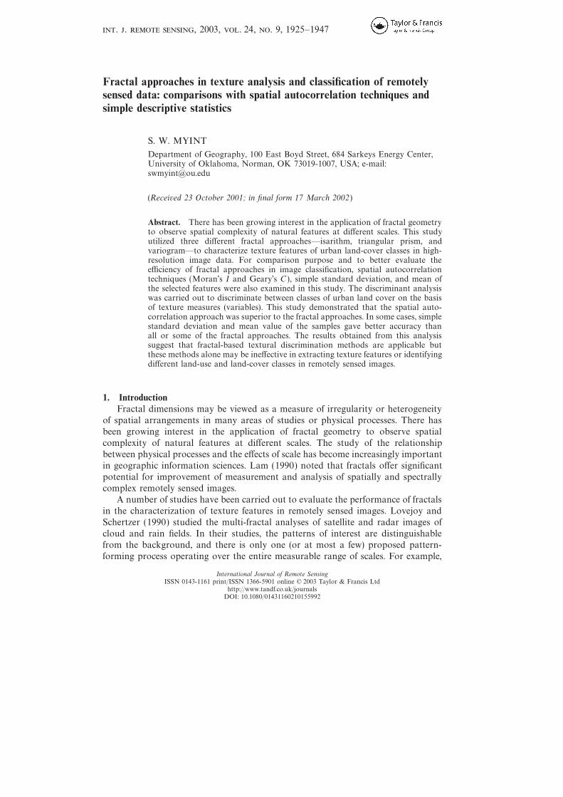
of Baton Rouge metropolitan area (southeast of Louisiana State University in thelower left part of the photo) is shown in band 2 (figure 1).
In this experiment, six urban land-cover features with different textural appear-ance were selected. It is often suggested that it would be preferable to choose trainingsites, where possible, according to some stratified random-sampling scheme. In thisstudy, a sample of 10 non-contiguous pixels was selected for each class from thesubset of Advanced Thermal Land Application Sensor (ATLAS) image data.
The selected land-cover classes in this research include single-family homes withless than 50% tree canopy (residential-1), single-family homes with more than 50%
Figure 1. A subset of the southern part of Baton Rouge metropolitan area (southeast ofLouisiana State University in the lower left part of the photo): band 2 (0.52–0.60 mm:visible green).
S. W. Myint1928
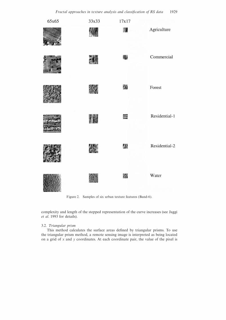
tree canopy (residential-2), commercial, woodland, agriculture, and water body. Twosegmented regions of each land-cover class were visually identified with the help oflocal area knowledge, ground information collection, and existing maps. Five trainingpixels were then randomly selected from each region, leading to a sample of 10pixels. Those pixels near class boundaries were not included in the random selectionprocess in order to avoid the problems associated with mixed class pixels andfeatures. The randomly selected samples were generated from relatively homogeneoustexture features. In this study, three different square window sizes centred at therandomly selected pixels in each region were used to generate training samples. Thewindow sizes include 17×17, 33×33, and 65×65. Criteria for the selection of windowsize are based on the resolution, minimum mapping unit size, classification specificity,and the nature of the classes (size of the regions, minimum number of pixels orminimum ground distance to cover a particular land-cover feature, directionality,and spatial periodicity) to be identified. It is understood that smaller window sizedoes not cover sufficient spatial/texture information to characterize land use types.However, if the window size is too large, too much information from other land-useand land-cover types could be included and hence the algorithm may not be effective.Samples of the classes generated from band-6 are shown in figure 2.
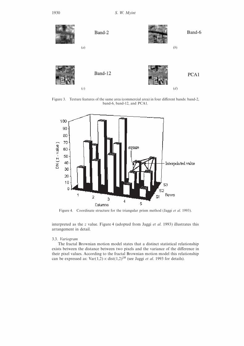
It was observed that textures of the same area in different bands (e.g. visible,reflected infrared, and thermal infrared) were different in terms of contrast, smooth-ness and coarseness, and spatial variation. Since different texture appearances of thesame area in different bands were observed, four different bands were selected andexamined in this study. Band-2 (0.52mm–0.60mm) was selected as it represents avisible band. Band-6 (0.76mm–0.90mm) was selected to represent a near infraredband, and band-12 (9.60mm–10.20mm) represents a thermal band. In addition tothese three bands, principal component analysis 1 (PCA1) was also examined in thisanalysis. Figure 3 shows the differences in texture features of the same area in fourdifferent bands: band-2, band-6, band-12, and PCA1 band.
3. Fractal measurementsThere have been numerous studies on the concepts and uses of fractals since
Mandelbrot coined the term in 1975 (Mandelbrot 1982). A potential use of fractalsis the analysis of image texture (De Cola 1989, De Jong and Burrough 1995). Inthese situations, it is commonly observed that the degree of roughness, or largebrightness differences in short spatial intervals, in an image or surface is a functionof scale and not of experimental technique. A number of fractal algorithms havebeen programmed into a software package known as the Image Characterizationand Modeling System (ICAMS) (Quattrochi et al. 1997, Lam et al. 1998) which wasused in this study to explore the texture features of the study area. ICAMS providesthe ability to calculate the fractal dimension of remotely sensed images using theisarithm method (Lam and De Cola 1993), the variogram (Mark and Aronson 1984),and the triangular prism methods (Clarke 1986).
3.1. IsarithmThe isarithm method is a two dimensional extension of the line divider method.
In the line divider method, the fractal dimension of a curve is measured usingdifferent step sizes that represent the segments necessary to traverse a curve (Lamand De Cola 1993). For an irregular curve, as step sizes become smaller, the
Fractal approaches in texture analysis and classification of RS data 1929
Figure 2. Samples of six urban texture features (Band-6).
complexity and length of the stepped representation of the curve increases (see Jaggiet al. 1993 for details).
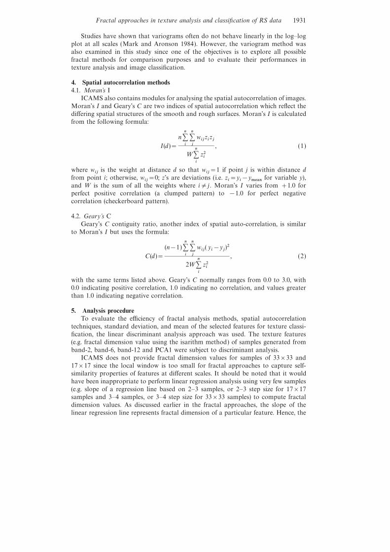
3.2. T riangular prismThis method calculates the surface areas defined by triangular prisms. To use
the triangular prism method, a remote sensing image is interpreted as being locatedon a grid of x and y coordinates. At each coordinate pair, the value of the pixel is
S. W. Myint1930
(a) (b)
(d)(c)
Figure 3. Texture features of the same area (commercial area) in four different bands: band-2,band-6, band-12, and PCA1.
Figure 4. Coordinate structure for the triangular prism method (Jaggi et al. 1993).
interpreted as the z value. Figure 4 (adopted from Jaggi et al. 1993) illustrates thisarrangement in detail.
3.3. VariogramThe fractal Brownian motion model states that a distinct statistical relationship
exists between the distance between two pixels and the variance of the difference intheir pixel values. According to the fractal Brownian motion model this relationshipcan be expressed as: Var(1,2)3dist(1,2)2H (see Jaggi et al. 1993 for details).
Fractal approaches in texture analysis and classification of RS data 1931
Studies have shown that variograms often do not behave linearly in the log–logplot at all scales (Mark and Aronson 1984). However, the variogram method wasalso examined in this study since one of the objectives is to explore all possiblefractal methods for comparison purposes and to evaluate their performances intexture analysis and image classification.
4. Spatial autocorrelation methods4.1. Moran’s I
ICAMS also contains modules for analysing the spatial autocorrelation of images.Moran’s I and Geary’s C are two indices of spatial autocorrelation which reflect thediffering spatial structures of the smooth and rough surfaces. Moran’s I is calculatedfrom the following formula:
I(d )=n∑n
i∑n
jwijzizj
W ∑n
iz2i
, (1)
where wij
is the weight at distance d so that wij=1 if point j is within distance d
from point i; otherwise, wij=0; z’s are deviations (i.e. z
i=yi−ymean for variable y),
and W is the sum of all the weights where i≠ j . Moran’s I varies from +1.0 forperfect positive correlation (a clumped pattern) to −1.0 for perfect negativecorrelation (checkerboard pattern).
4.2. Geary’s CGeary’s C contiguity ratio, another index of spatial auto-correlation, is similar
to Moran’s I but uses the formula:
C(d )=(n−1)∑
n
i∑n
jwij( yi−yj)2
2W ∑n
iz2i
, (2)
with the same terms listed above. Geary’s C normally ranges from 0.0 to 3.0, with0.0 indicating positive correlation, 1.0 indicating no correlation, and values greaterthan 1.0 indicating negative correlation.
5. Analysis procedureTo evaluate the efficiency of fractal analysis methods, spatial autocorrelation
techniques, standard deviation, and mean of the selected features for texture classi-fication, the linear discriminant analysis approach was used. The texture features(e.g. fractal dimension value using the isarithm method) of samples generated fromband-2, band-6, band-12 and PCA1 were subject to discriminant analysis.
ICAMS does not provide fractal dimension values for samples of 33×33 and17×17 since the local window is too small for fractal approaches to capture self-similarity properties of features at different scales. It should be noted that it wouldhave been inappropriate to perform linear regression analysis using very few samples(e.g. slope of a regression line based on 2–3 samples, or 2–3 step size for 17×17samples and 3–4 samples, or 3–4 step size for 33×33 samples) to compute fractaldimension values. As discussed earlier in the fractal approaches, the slope of thelinear regression line represents fractal dimension of a particular feature. Hence, the
S. W. Myint1932
accuracy of the fractal analysis for samples of 33×33 and 17×17 were not availablein this analysis. However, the results of spatial autocorrelation, simple standarddeviation, and mean value of the 33×33 and 17×17 samples are presented anddiscussed.
The discriminant analysis was carried out to discriminate between classes ofurban land cover on the basis of texture measures (variables). For example, thefractal dimension values of samples generated from band-6 were treated as variablesto identify features of urban land cover classes. Linear discriminant procedure in theMinitab software package was used to investigate the relative discriminatory powerof all variables and to determine classification accuracies for different variable com-binations. The discriminant analysis was carried out to discriminate between texturalfeatures of urban land cover on the basis of the values measured from the fractalmethods (isarithm, triangular prism, and variogram), spatial autocorrelation tech-niques (Moran’s I and Geary’s C ), simple descriptive statistics (mean and standarddeviation).
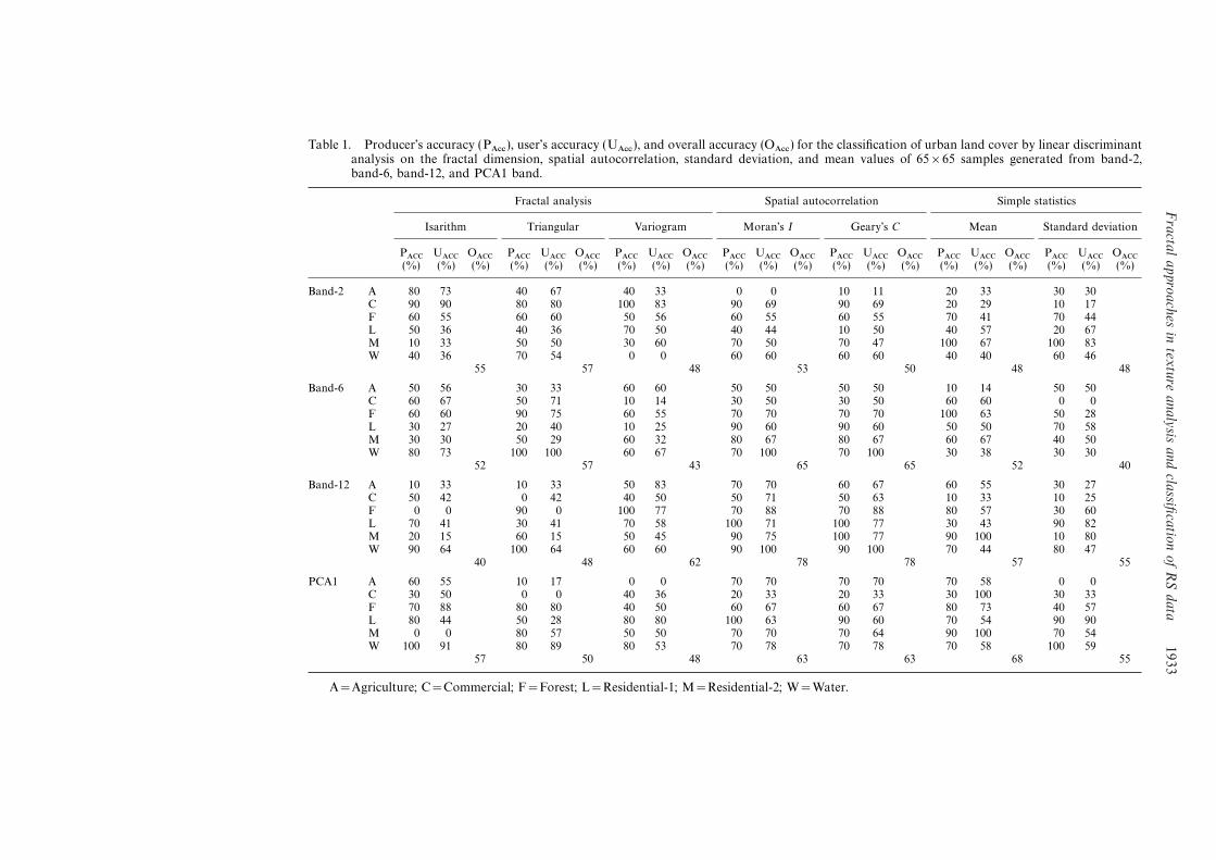
6. Results and discussionTable 1 shows the accuracies—producer’s accuracy (PAcc ), user’s accuracy (UAcc ),
and overall accuracy (OAcc)—for the discrimination of the classes of urban land coverby linear discriminant analysis on the fractal dimensions, spatial autocorrelation,standard deviation, and mean values of the samples of 65×65 derived from band-2,band-6, and band-12. It can be seen from table 1 that different classes reach theirmaximum producer’s, user’s, and overall accuracies with different techniques.
The highest accuracy of all methods for band-2 using 65×65 samples wasproduced by the triangular prism method (57%). It is observed that there is significantconfusion between residential-1 and residential-2. Geary’s C produced the lowestaccuracy (50%). Moreover, the lowest producer’s accuracy (0%) and user’s accuracy(0%) were also found with agriculture in Moran’s I method. In general, the overallclassification accuracy for isarithm, triangular prism, Moran’s I, Geary’s C, standarddeviation, and mean for band-2 were found to be 55%, 57%, 53%, 50%, 48%,and 48% respectively. The only highly reliable category associated with fractal andspatial autocorrelation technique is commercial in this analysis. However, it was notconsistent with what was found in standard deviation and mean of the samples.Residential-2 was the most highly reliable category in this case.
The highest accuracy of all methods for band-6 using 65×65 samples wasproduced by Moran’s I and Geary’s C (65%). Water body was found to be the mostreliable category for the isarithm, triangular prism, and variogram methods whereasresidential-1 produced the highest accuracy for Moran’s I and Geary’s C. The lowestproducer’s accuracy and user’s accuracy were produced by the isarithm and triangularprism methods associated with the residential-1 and residential-2 land-cover classes.There is some confusion among the commercial, residential-1, and residential-2 forthe fractal methods. There is also some confusion between agriculture and commercialfor the spatial autcorrelation methods. The overall classification accuracy for isar-ithm, triangular prism, variogram, Moran’s I, Geary’s C, standard deviation, andmean for band-6 were found to be 52%, 57%, 43%, 65%, 65%, 52%, and 40%,respectively. In general, the spatial autocorrelation techniques are more accuratethan the fractal methods with band-6 data.
The highest accuracy of all methods for band-12 using 65×65 samples was againproduced by Moran’s I and Geary’s C (78%). There is significant confusion between
FractalapproachesintextureanalysisandclassificationofRSdata
1933
Table 1. Producer’s accuracy (PAcc ), user’s accuracy (UAcc ), and overall accuracy (OAcc ) for the classification of urban land cover by linear discriminantanalysis on the fractal dimension, spatial autocorrelation, standard deviation, and mean values of 65×65 samples generated from band-2,band-6, band-12, and PCA1 band.
Fractal analysis Spatial autocorrelation Simple statistics
Isarithm Triangular Variogram Moran’s I Geary’s C Mean Standard deviation
PACC UACC OACC PACC UACC OACC PACC UACC OACC PACC UACC OACC PACC UACC OACC PACC UACC OACC PACC UACC OACC(%) (%) (%) (%) (%) (%) (%) (%) (%) (%) (%) (%) (%) (%) (%) (%) (%) (%) (%) (%) (%)
Band-2 A 80 73 40 67 40 33 0 0 10 11 20 33 30 30C 90 90 80 80 100 83 90 69 90 69 20 29 10 17F 60 55 60 60 50 56 60 55 60 55 70 41 70 44L 50 36 40 36 70 50 40 44 10 50 40 57 20 67M 10 33 50 50 30 60 70 50 70 47 100 67 100 83W 40 36 70 54 0 0 60 60 60 60 40 40 60 46
55 57 48 53 50 48 48
Band-6 A 50 56 30 33 60 60 50 50 50 50 10 14 50 50C 60 67 50 71 10 14 30 50 30 50 60 60 0 0F 60 60 90 75 60 55 70 70 70 70 100 63 50 28L 30 27 20 40 10 25 90 60 90 60 50 50 70 58M 30 30 50 29 60 32 80 67 80 67 60 67 40 50W 80 73 100 100 60 67 70 100 70 100 30 38 30 30
52 57 43 65 65 52 40
Band-12 A 10 33 10 33 50 83 70 70 60 67 60 55 30 27C 50 42 0 42 40 50 50 71 50 63 10 33 10 25F 0 0 90 0 100 77 70 88 70 88 80 57 30 60L 70 41 30 41 70 58 100 71 100 77 30 43 90 82M 20 15 60 15 50 45 90 75 100 77 90 100 10 80W 90 64 100 64 60 60 90 100 90 100 70 44 80 47
40 48 62 78 78 57 55
PCA1 A 60 55 10 17 0 0 70 70 70 70 70 58 0 0C 30 50 0 0 40 36 20 33 20 33 30 100 30 33F 70 88 80 80 40 50 60 67 60 67 80 73 40 57L 80 44 50 28 80 80 100 63 90 60 70 54 90 90M 0 0 80 57 50 50 70 70 70 64 90 100 70 54W 100 91 80 89 80 53 70 78 70 78 70 58 100 59
57 50 48 63 63 68 55
A=Agriculture; C=Commercial; F=Forest; L=Residential-1; M=Residential-2; W=Water.
S. W. Myint1934
agriculture and commercial. The isarithm method produced the lowest overall accu-racy (40%). The lowest producer’s accuracy (0%) and user’s accuracy (0%) wereproduced by the isarithm and triangular prism methods associated with the woodlandand commercial land cover. The variogram gave the highest accuracy (62%) amongall fractal approaches for all bands in this analysis. In general, the overall classificationaccuracy for isarithm, triangular prism, variogram, Moran’s I, Geary’s C, standarddeviation, and mean for band-12 were found to be 40%, 48%, 62%, 78%, 78%,57%, and 55%, respectively. Woodland was found to be one of the most reliablecategories (user’s accuracy=100%, producer’s accuracy=90%) in the triangularprism method. It was found to be the least efficient category (user’s accuracy=0%,producer’s accuracy=0%) in the isarithm method. It has been observed that a classthat gives the highest accuracy in one band may give the lowest accuracy in anotherband when using fractal approaches. Moreover, a category that seems to be mostreliable in one method could produce the lowest accuracy in another fractal methodusing the same band. In general, the spatial autocorrelation techniques are againmore efficient than the fractal methods with band-12 data. In contrast to the previousfindings with band-2 and band-6, overall accuracy produced by variogram methodwas found to be higher than isarithm and triangular prism methods.
The highest accuracy of all methods for PCA1 using 65×65 samples was pro-duced by the mean values of the samples of 65×65 (68%). The variogram methodproduced the lowest overall accuracy (48%). The lowest producer’s accuracies (0%)found in the analysis were produced by the isarithm method for residential-2 andthe triangular prism method for commercial. There are also similar situationsobserved for some other classes in fractal methods. This finding is disappointingsince no single individual class accuracy is consistent with the methods used. It ishard to make a conclusion on which category is most reliable and which categoryis most problematic since individual class performance in the classification variedgreatly by the methods used. It is also hard to determine the class confusion for thesame reason. However, residential-2 was found to be the most reliable category withthe highest producer’s accuracy (80%) in the triangular prism method. Residential-1produced the highest producer’s accuracy (100%) in Moran’s I method.
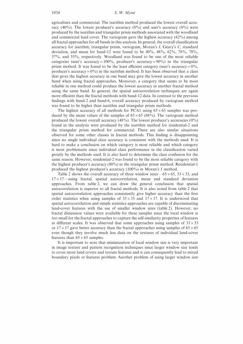
Table 2 shows the overall accuracy of three window sizes—65×65, 33×33, and17×17—using fractal, spatial autocorrelation, mean and standard deviationapproaches. From table 2, we can draw the general conclusion that spatialautocorrelation is superior to all fractal methods. It is also noted from table 2 thatspatial autocorrelation approaches consistently give higher accuracy than the firstorder statistics when using samples of 33×33 and 17×17. It is understood thatspatial autocorrelation and simple statistics approaches are capable of discriminatingland-cover features with the use of smaller window sizes (table 2). However, nofractal dimension values were available for these samples since the local window istoo small for the fractal approaches to capture the self-similarity properties of featuresat different scales. It was observed that some approaches using samples of 33×33or 17×17 gave better accuracy than the fractal approaches using samples of 65×65even though they involve much less data on the textures of individual land-coverfeatures than 65×65 samples.
It is important to note that minimization of local window size is very importantin image texture and pattern recognition techniques since larger window size tendsto cover more land covers and texture features and it can consequently lead to mixedboundary pixels or features problem. Another problem of using larger window size
Fractal approaches in texture analysis and classification of RS data 1935
Table 2. Overall accuracies for all bands for three window sizes: 65×65, 33×33, and 17×17using fractal, spatial autocorrelation, mean and standard deviation approaches.
Overall accuracy (%)
Sample Moran’s Geary’s Standardsize Band Isarithm Triangular Variogram I C Mean deviation
65×65 Band-2 55 57 48 53 50 48 48Band-6 52 57 43 65 65 52 41Band-12 40 48 62 78 78 57 55PCA1 57 50 48 65 63 68 55
33×33 Band-2 — — — 53 57 47 40Band-6 — — — 60 62 48 42Band-12 — — — 57 55 53 50PCA1 — — — 50 48 55 45
17×17 Band-2 — — — 47 42 25 28Band-6 — — — 52 53 25 27Band-12 — — — 55 58 38 32PCA1 — — — 45 45 33 33
is the fact that smaller land-cover features will not be identified in classification. Inother words the smaller the window size the larger the number of segmented regionsor land cover features extracted. It will also maximize missing pixels on the edgessuch as 15 missing pixels on the left, right, top and bottom of the image for 33×33window size (Gong and Howarth 1992, Kershaw and Fuller 1992, Gong 1994,Hodgson 1998, Pesaresi 2000, Myint 2001).
It was observed from table 1 that the lowest overall accuracy of all approachesfor all bands with the samples of 65×65 was produced by isarithm method (40%)and the highest overall accuracy was produced by two spatial autocorrelation tech-niques (78%) when using band-12. Variogram gave the highest accuracy (62%)among all fractal approaches for all bands in this analysis. This finding was notconsistent with what was noted by Lam (1990) in the description and measurementof Landsat TM images using fractals. However, variogram should not be recognizedas the most effective of all fractal approaches. It gave lower accuracies than otherapproaches when using other bands. It is hard to make a decision on which fractalmethod is most reliable and which category is most problematic since individualclass performance in the classification varied greatly by all fractal methods used. Theoverall accuracies for all bands also varied greatly by these methods.
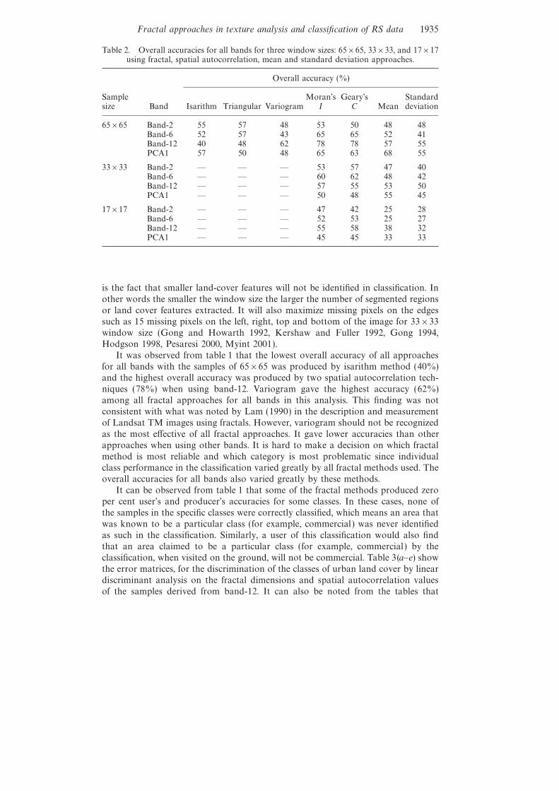
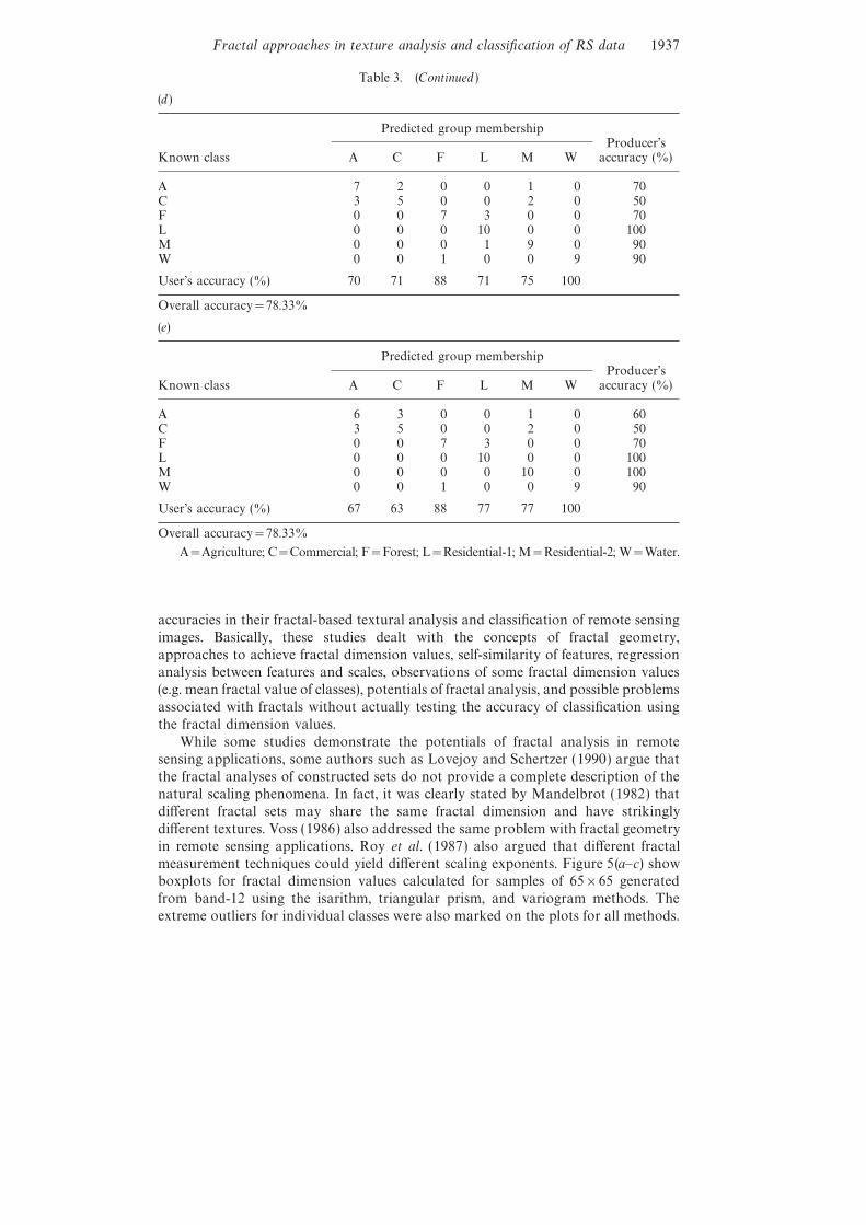
It can be observed from table 1 that some of the fractal methods produced zeroper cent user’s and producer’s accuracies for some classes. In these cases, none ofthe samples in the specific classes were correctly classified, which means an area thatwas known to be a particular class (for example, commercial ) was never identifiedas such in the classification. Similarly, a user of this classification would also findthat an area claimed to be a particular class (for example, commercial ) by theclassification, when visited on the ground, will not be commercial. Table 3(a–e) showthe error matrices, for the discrimination of the classes of urban land cover by lineardiscriminant analysis on the fractal dimensions and spatial autocorrelation valuesof the samples derived from band-12. It can also be noted from the tables that
S. W. Myint1936
Table 3. Error matrices for linear discriminant analysis of urban land cover features usingfractal dimensions and spatial autocorrelations of 65×65 samples generated fromband-12. (a) isarithm method, (b) triangular prism method, (c) variogram, (d) Moran’sI, (e) Geary’s C.
(a)
Predicted group membershipProducer’s
Known class A C F L M W accuracy (%)
A 1 5 0 1 3 0 10C 1 5 0 1 3 0 50F 0 0 0 3 2 5 0L 0 0 0 7 3 0 70M 1 2 1 4 2 0 20W 0 0 0 1 0 9 90
User’s accuracy (%) 33 42 0 41 15 64
Overall accuracy=40.00%
(b)
Predicted group membershipProducer’s
Known class A C F L M W accuracy (%)
A 1 2 0 6 1 0 10C 0 0 0 5 5 0 0F 0 0 9 1 0 0 90L 3 3 0 3 1 0 30M 0 4 0 0 6 0 60W 0 0 0 0 0 10 100
User’s accuracy (%) 25 0 100 20 46 100
Overall accuracy=48.33%
(c)
Predicted group membershipProducer’s
Known class A C F L M W accuracy (%)
A 5 0 3 0 0 2 50C 0 4 0 2 3 1 40F 0 0 10 0 0 0 100L 0 3 0 7 0 0 70M 0 1 0 3 5 1 50W 1 0 0 0 3 6 60
User’s accuracy (%) 83 50 77 58 45 60
Overall accuracy=61.67%
different land cover classes reach their maximum producer’s, user’s and overallclassification accuracies with different techniques.
As mentioned earlier, a number of studies have been carried out to examine theperformance of fractal geometry in applications of remotely sensed images. Most ofthe studies did not evaluate the performance and did not provide the classification
Fractal approaches in texture analysis and classification of RS data 1937
Table 3. (Continued )
(d )
Predicted group membershipProducer’s
Known class A C F L M W accuracy (%)
A 7 2 0 0 1 0 70C 3 5 0 0 2 0 50F 0 0 7 3 0 0 70L 0 0 0 10 0 0 100M 0 0 0 1 9 0 90W 0 0 1 0 0 9 90
User’s accuracy (%) 70 71 88 71 75 100
Overall accuracy=78.33%
(e)
Predicted group membershipProducer’s
Known class A C F L M W accuracy (%)
A 6 3 0 0 1 0 60C 3 5 0 0 2 0 50F 0 0 7 3 0 0 70L 0 0 0 10 0 0 100M 0 0 0 0 10 0 100W 0 0 1 0 0 9 90
User’s accuracy (%) 67 63 88 77 77 100
Overall accuracy=78.33%
A=Agriculture; C=Commercial; F=Forest; L=Residential-1; M=Residential-2; W=Water.
accuracies in their fractal-based textural analysis and classification of remote sensingimages. Basically, these studies dealt with the concepts of fractal geometry,approaches to achieve fractal dimension values, self-similarity of features, regressionanalysis between features and scales, observations of some fractal dimension values(e.g. mean fractal value of classes), potentials of fractal analysis, and possible problemsassociated with fractals without actually testing the accuracy of classification usingthe fractal dimension values.
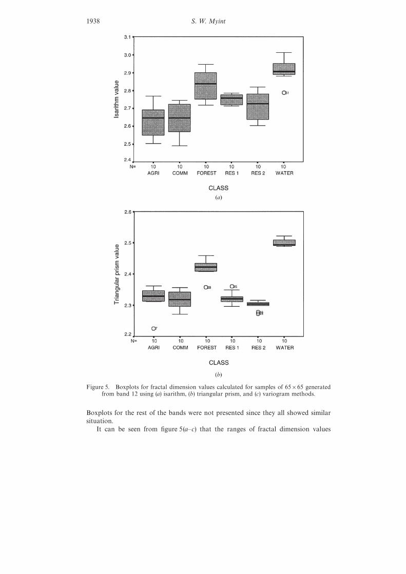
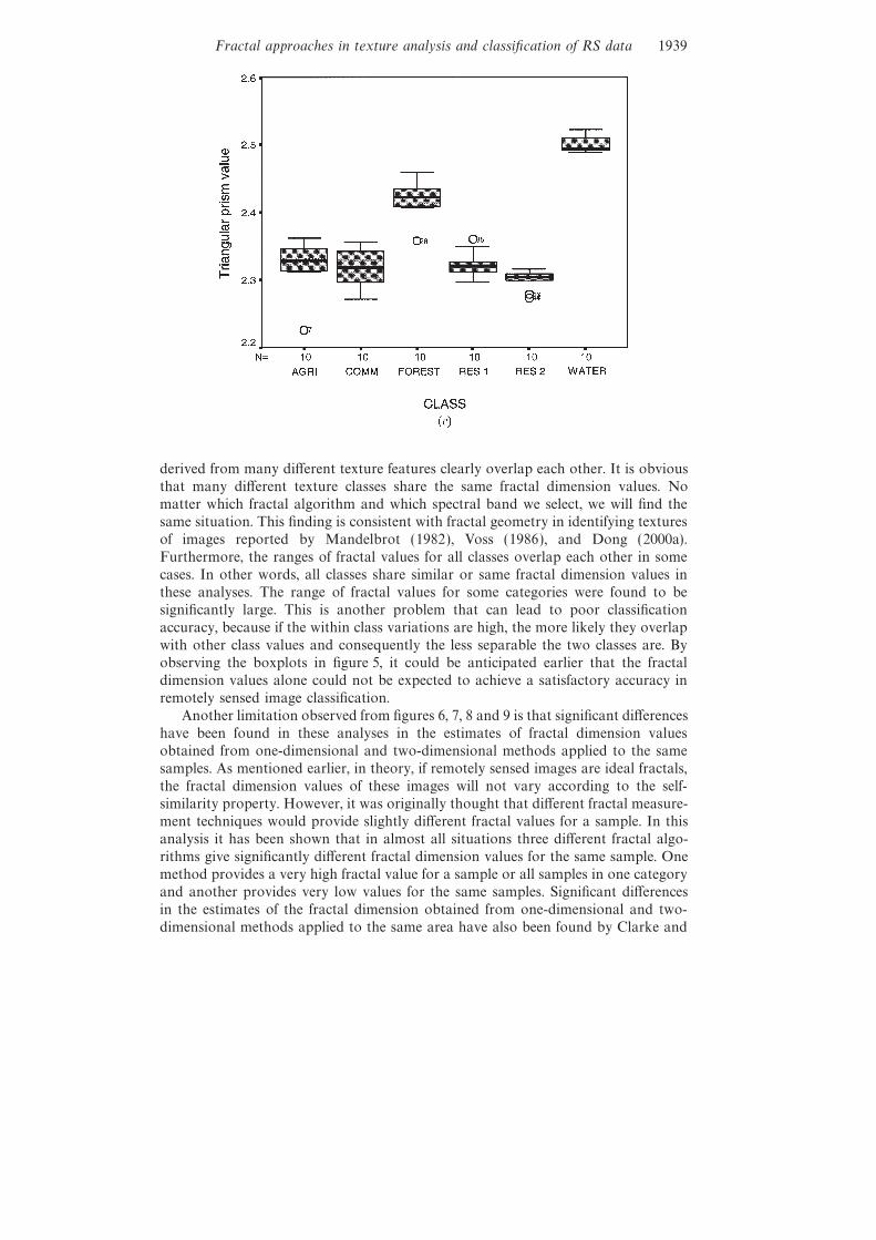
While some studies demonstrate the potentials of fractal analysis in remotesensing applications, some authors such as Lovejoy and Schertzer (1990) argue thatthe fractal analyses of constructed sets do not provide a complete description of thenatural scaling phenomena. In fact, it was clearly stated by Mandelbrot (1982) thatdifferent fractal sets may share the same fractal dimension and have strikinglydifferent textures. Voss (1986) also addressed the same problem with fractal geometryin remote sensing applications. Roy et al. (1987) also argued that different fractalmeasurement techniques could yield different scaling exponents. Figure 5(a–c) showboxplots for fractal dimension values calculated for samples of 65×65 generatedfrom band-12 using the isarithm, triangular prism, and variogram methods. Theextreme outliers for individual classes were also marked on the plots for all methods.
S. W. Myint1938
Figure 5. Boxplots for fractal dimension values calculated for samples of 65×65 generatedfrom band 12 using (a) isarithm, (b) triangular prism, and (c) variogram methods.
Boxplots for the rest of the bands were not presented since they all showed similarsituation.
It can be seen from figure 5(a–c) that the ranges of fractal dimension values
Fractal approaches in texture analysis and classification of RS data 1939
derived from many different texture features clearly overlap each other. It is obviousthat many different texture classes share the same fractal dimension values. Nomatter which fractal algorithm and which spectral band we select, we will find thesame situation. This finding is consistent with fractal geometry in identifying texturesof images reported by Mandelbrot (1982), Voss (1986), and Dong (2000a).Furthermore, the ranges of fractal values for all classes overlap each other in somecases. In other words, all classes share similar or same fractal dimension values inthese analyses. The range of fractal values for some categories were found to besignificantly large. This is another problem that can lead to poor classificationaccuracy, because if the within class variations are high, the more likely they overlapwith other class values and consequently the less separable the two classes are. Byobserving the boxplots in figure 5, it could be anticipated earlier that the fractaldimension values alone could not be expected to achieve a satisfactory accuracy inremotely sensed image classification.
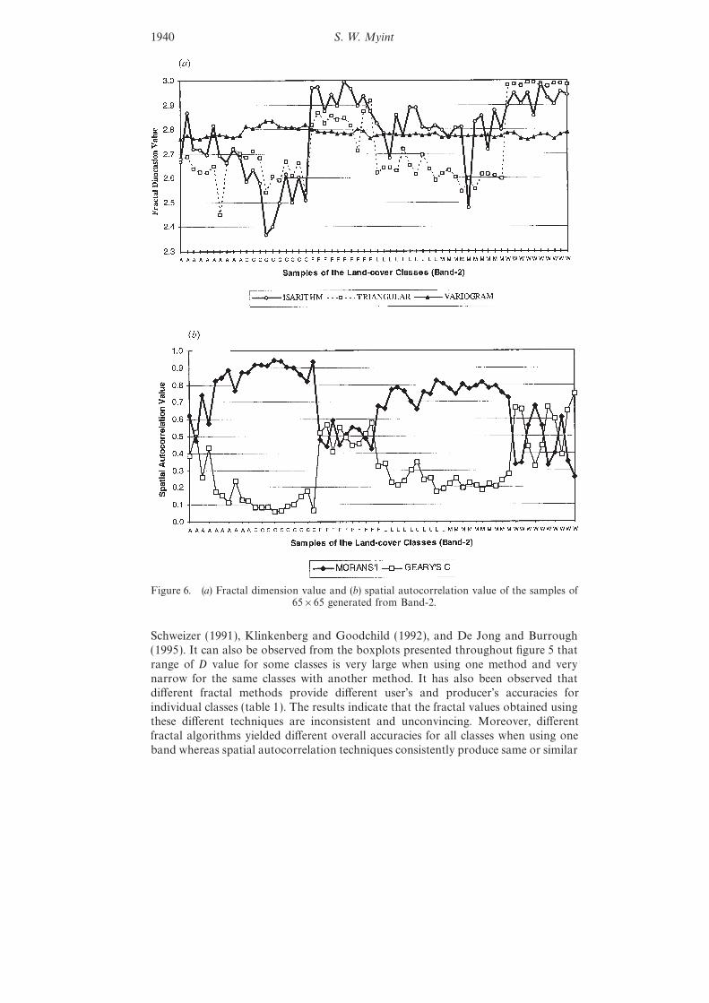
Another limitation observed from figures 6, 7, 8 and 9 is that significant differenceshave been found in these analyses in the estimates of fractal dimension valuesobtained from one-dimensional and two-dimensional methods applied to the samesamples. As mentioned earlier, in theory, if remotely sensed images are ideal fractals,the fractal dimension values of these images will not vary according to the self-similarity property. However, it was originally thought that different fractal measure-ment techniques would provide slightly different fractal values for a sample. In thisanalysis it has been shown that in almost all situations three different fractal algo-rithms give significantly different fractal dimension values for the same sample. Onemethod provides a very high fractal value for a sample or all samples in one categoryand another provides very low values for the same samples. Significant differencesin the estimates of the fractal dimension obtained from one-dimensional and two-dimensional methods applied to the same area have also been found by Clarke and
S. W. Myint1940
Figure 6. (a) Fractal dimension value and (b) spatial autocorrelation value of the samples of65×65 generated from Band-2.
Schweizer (1991), Klinkenberg and Goodchild (1992), and De Jong and Burrough(1995). It can also be observed from the boxplots presented throughout figure 5 thatrange of D value for some classes is very large when using one method and verynarrow for the same classes with another method. It has also been observed thatdifferent fractal methods provide different user’s and producer’s accuracies forindividual classes (table 1). The results indicate that the fractal values obtained usingthese different techniques are inconsistent and unconvincing. Moreover, differentfractal algorithms yielded different overall accuracies for all classes when using oneband whereas spatial autocorrelation techniques consistently produce same or similar
Fractal approaches in texture analysis and classification of RS data 1941
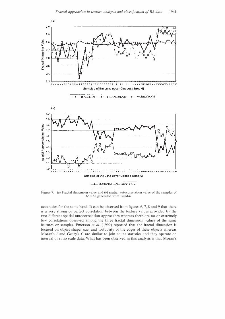
Figure 7. (a) Fractal dimension value and (b) spatial autocorrelation value of the samples of65×65 generated from Band-6.
accuracies for the same band. It can be observed from figures 6, 7, 8 and 9 that thereis a very strong or perfect correlation between the texture values provided by thetwo different spatial autocorrelation approaches whereas there are no or extremelylow correlations observed among the three fractal dimension values of the samefeatures or samples. Emerson et al. (1999) reported that the fractal dimension isfocused on object shape, size, and tortuosity of the edges of these objects whereasMoran’s I and Geary’s C are similar to join count statistics and they operate oninterval or ratio scale data. What has been observed in this analysis is that Moran’s
S. W. Myint1942
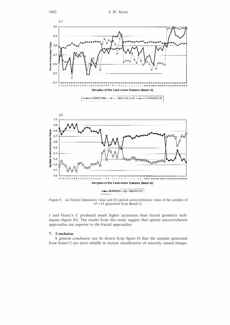
Figure 8. (a) Fractal dimension value and (b) spatial autocorrelation value of the samples of65×65 generated from Band-12.
I and Geary’s C produced much higher accuracies than fractal geometry tech-niques (figure 10). The results from this study suggest that spatial autocorrelationapproaches are superior to the fractal approaches.
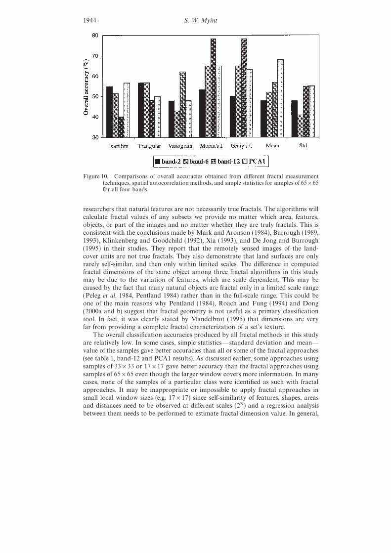
7. ConclusionA general conclusion can be drawn from figure 10 that the samples generated
from band-12 are most reliable in texture classification of remotely sensed images.
Fractal approaches in texture analysis and classification of RS data 1943
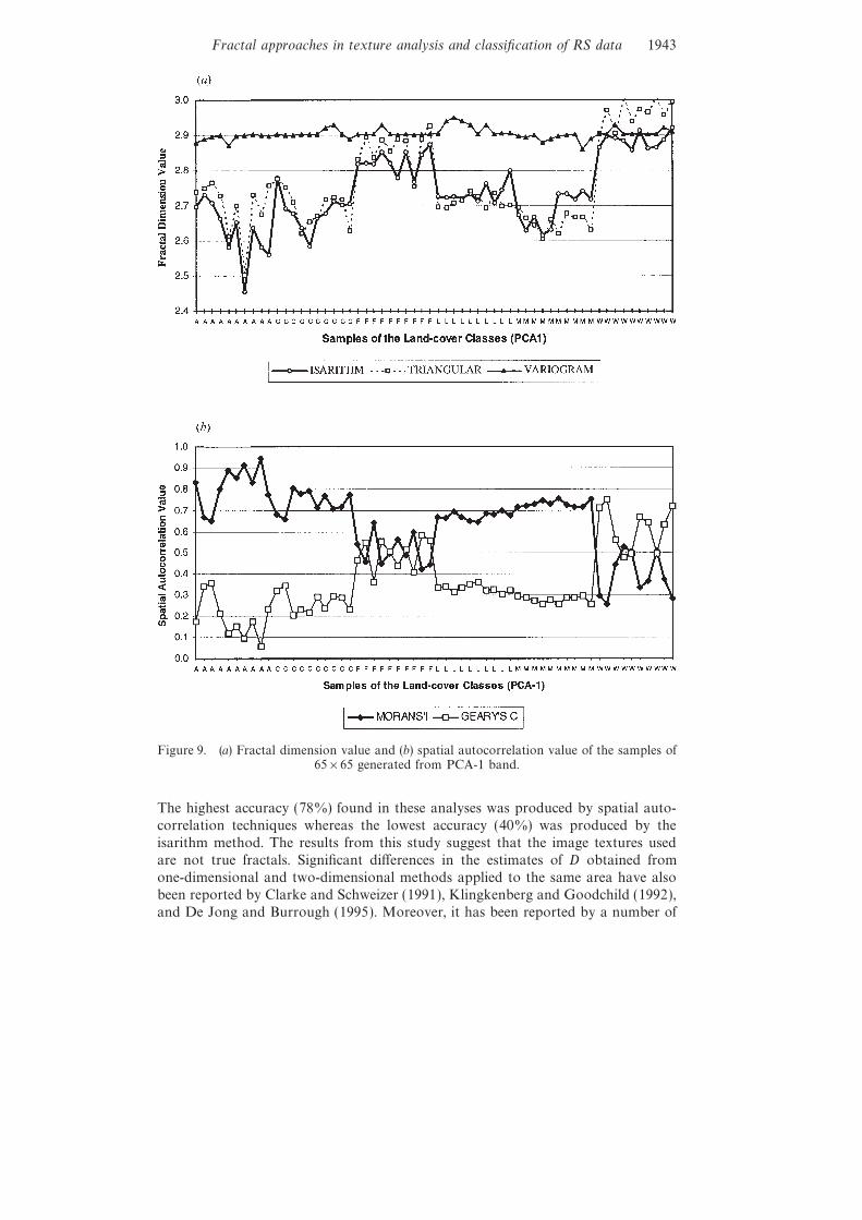
Figure 9. (a) Fractal dimension value and (b) spatial autocorrelation value of the samples of65×65 generated from PCA-1 band.
The highest accuracy (78%) found in these analyses was produced by spatial auto-correlation techniques whereas the lowest accuracy (40%) was produced by theisarithm method. The results from this study suggest that the image textures usedare not true fractals. Significant differences in the estimates of D obtained fromone-dimensional and two-dimensional methods applied to the same area have alsobeen reported by Clarke and Schweizer (1991), Klingkenberg and Goodchild (1992),and De Jong and Burrough (1995). Moreover, it has been reported by a number of
S. W. Myint1944
Figure 10. Comparisons of overall accuracies obtained from different fractal measurementtechniques, spatial autocorrelation methods, and simple statistics for samples of 65×65for all four bands.
researchers that natural features are not necessarily true fractals. The algorithms willcalculate fractal values of any subsets we provide no matter which area, features,objects, or part of the images and no matter whether they are truly fractals. This isconsistent with the conclusions made by Mark and Aronson (1984), Burrough (1989,1993), Klinkenberg and Goodchild (1992), Xia (1993), and De Jong and Burrough(1995) in their studies. They report that the remotely sensed images of the land-cover units are not true fractals. They also demonstrate that land surfaces are onlyrarely self-similar, and then only within limited scales. The difference in computedfractal dimensions of the same object among three fractal algorithms in this studymay be due to the variation of features, which are scale dependent. This may becaused by the fact that many natural objects are fractal only in a limited scale range(Peleg et al. 1984, Pentland 1984) rather than in the full-scale range. This could beone of the main reasons why Pentland (1984), Roach and Fung (1994) and Dong(2000a and b) suggest that fractal geometry is not useful as a primary classificationtool. In fact, it was clearly stated by Mandelbrot (1995) that dimensions are veryfar from providing a complete fractal characterization of a set’s texture.
The overall classification accuracies produced by all fractal methods in this studyare relatively low. In some cases, simple statistics—standard deviation and mean—value of the samples gave better accuracies than all or some of the fractal approaches(see table 1, band-12 and PCA1 results). As discussed earlier, some approaches usingsamples of 33×33 or 17×17 gave better accuracy than the fractal approaches usingsamples of 65×65 even though the larger window covers more information. In manycases, none of the samples of a particular class were identified as such with fractalapproaches. It may be inappropriate or impossible to apply fractal approaches insmall local window sizes (e.g. 17×17) since self-similarity of features, shapes, areasand distances need to be observed at different scales (2N ) and a regression analysisbetween them needs to be performed to estimate fractal dimension value. In general,
Fractal approaches in texture analysis and classification of RS data 1945
spatial autocorrelation methods were found to be more accurate than fractalapproaches. It is recommended that other widely accepted and well-known window-based techniques for incorporating spatial information in image classification(Franklin and Peddle 1987, Wang and He 1990, Gong et al. 1992, Pesaresi 2000) beexamined and compared.
From the preceding discussion and conclusion, a checklist of the sources oflimitation or uncertainty in the application of fractal based texture measures toremotely sensed image classification may be identified as follows.
$ Different fractal measurement techniques may yield different fractal dimensionsof the same object.
$ Different objects and land-cover features may share the same fractal dimensionvalue and have completely different textures.
$ A local window must be sufficiently large to perform a regression on thelogarithm of number of edges or total surface areas or variance against thelogarithm of the cell size/step size/scale (2N ). However, it should be noted thatminimization of local window size is required for better accuracy in imageclassification.
$ The remotely sensed images of the land-cover units may not be true fractalsand many natural objects are fractal only in a limited range. It has also beenreported that natural features and phenomena are not necessarily self-similar.
$ The application of fractal approaches to samples, subsets, and/or images with-out examining whether they are truly fractal may lead to poor results. However,if we are to check whether samples or features in local windows are true fractalsand apply the fractal approaches only to the features identified as true fractals,texture analysis and image classification would not be possible since no resultswill be available for those local windows or subsets identified as non-fractals.
$ The fractal dimension values may vary significantly for a feature/subsetdepending on parameter inputs specified within a method (e.g. steps, distance,interval, orientation, calculation techniques).
$ Fractal dimensions obtained for the samples of the same feature class may varysignificantly. The regression analysis between features/areas, and scales to obtainslope yields only information on the average scaling property of textures.
It is obvious from the above discussion that the fractal dimension describes onlypart of the information in the distribution of spatial features. Future research isrequired to evaluate other alternative approaches such as lacunarity (Voss 1986,Mandelbrot 1995, Dong 2000a, b), which could describe the characteristics of fractalsof the same dimension with different texture appearances.
AcknowledgmentsThis research was supported by the Otis Paul Starkey Fund (The Association of
American Geographers) under the AAG grants/awards and the Robert C. West fieldresearch grant (Department of Geography and Anthropology, LSU). This work wasmade possible by the help and inspiration of Nina Lam, Department of Geographyand Anthropology, LSU. The author thanks Nina Lam and Wei Zhao, Departmentof Geography and Anthropology, LSU for the ICAMS program. The author alsoexpresses his appreciation to DeWitt Braud, Department of Geography andAnthropology, LSU for providing the ATLAS data for this study and reviewing thedraft manuscript.
S. W. Myint1946
ReferencesB, P. A., 1989, Fractals and geochemistry. In T he Fractal Approaches to
Heterogeneous Chemistry, edited by D. Avnir (New York: Wiley & Sons Ltd),pp. 383–405.
B, P. A., 1993, Soil variability: a late 20th century view. Soils and Fertilizers, 56,529–562.
C, K. C., 1986, Computation of the fractal dimension of topographic surfaces using thetriangular prism surface area method. Computers and Geosciences, 12, 713–722.
C, K. C., and S, D. M., 1991, Measuring the fractal dimension of naturalsurfaces using a robust fractal estimator. Cartography and Geographic InformationSystems, 18, 37–47.
D C, L., 1989, Fractal analysis of a classified Landsat scene. Photogrammetric Engineeringand Remote Sensing, 55, 601–610.
D J, S. M., and B, P. A., 1995, A fractal approach to the classification ofMediterranean vegetation types in remotely sensed images. PhotogrammetricEngineering and Remote Sensing, 61, 1041–1053.
D, P., 2000a, Lacunarity for Spatial Heterogeneity Measurement in GIS. GeographicInformation Sciences, 6, 20–26.
D, P., 2000b, Test of a new lacunarity estimation method for image texture analysis.International Journal of Remote Sensing, 17, 3369–3373.
E, C. W., L, N. S. N., and Q, D. A., 1999, Multi-scale fractal analysis ofimage texture and pattern. Photogrammetric Engineering and Remote Sensing, 65, 51–61.
F, S. E., and P, D., 1987, Texture analysis of digital image data using spatialcooccurrence. Computer and Geosciences, 13, 293–311.
G, P., and H, P. J., 1992, Frequency based contextual classification and gray levelvector reduction for land use identification. Photogrammetric Engineering and RemoteSensing, 58, 423–437.
G, P., 1994, Reducing boundary effects in a kernel-based classifier. International Journalof Remote Sensing, 15, 1131–1139.
G, P., M, D. J., and H, P. J., 1992, A comparison of spatial featureextraction algorithms for land-use classification with SPOT HRV data. Remote Sensingof Environment, 40, 137–151.
H, M. E., 1998, What size window for image classification? A cognitive perspective.Photogrammetric Engineering and Remote Sensing, 64, 797–807.
J, S., Q, D. A., and L, N. S. N., 1993, Implementation and operation ofthree fractal measurement algorithms for analysis of remote-sensing data. Computerand Geosciiences, 19, 745–767.
K, C. D., and F, R. M., 1992, Statistical problems in the discrimination of landcover from satellite images: a case in lowland Britain. International Journal of RemoteSensing, 13, 3085–3104.
K, B., and G, M. F., 1992, The fractal properties of topography: acomparison of methods. Earth Surface Processes and L andforms, 17, 217–234.
L, N. S. N., 1990, Description and measurement of Landsat TM images using fractals.Photogrammetric Engineering and Remote Sensing, 56, 187–195.
L, N. S. N., and D C, L., 1993, Fractal simulation and interpolation. In Fractals inGeography, edited by N. S. N. Lam and L. De Cola (Englewood Cliffs, NJ: PrenticeHall ), pp. 56–74.
L, N. S. N, Q, D., Q, H., and Z, W., 1998, Environmental assessment andmonitoring with image characterization and modeling system using multiscale remotesensing data. Applied Geographic Studies, 2, 77–93.
L, S., and S, D., 1990, Multifractals, universality classes and satellite andradar measurements of cloud and rain fields. Journal of Geophysical Research, 95,2021–2034.
M, B., 1982, T he Fractal Geometry of Nature (New York, NY: Freeman and Co).M, B. B., 1987, Fractals. In Encyclopedia of Physical Science and T echnology, Vol. 5,
edited by Robert A. Meyers (San Diego, CA: Academic Press), pp. 579–593.M, B., 1995, Measures of fractal lacunarity: Minkowski content and alternatives.
Progress in Probability, 37, 15–42.
Fractal approaches in texture analysis and classification of RS data 1947
M, D. M., and A, P. B., 1984, Scale dependent fractal dimensions of topographicsurfaces: an empirical investigation with applications in geomorphology and computermapping. Mathematical Geology, 16, 671–683.
M, S. W., 2001a, Wavelet Analysis and Classification of Urban Environment Using High-resolution Multispectral Image Data. Ph.D. dissertation, Louisiana State University,329 pp.
N, V. M., and Y R, V., 1992, Fractal dimension of ocean wave-breaking fromoptical data. European Geophysical Society, Annales Geophysicae, Part II; Oceans,Atmospheres, Hydrology and Nonlinear Geophysics, supplement II to Vol. 10, p. C343.
P, S., N, J., H, R., and A, D. D., 1984, Multiple resolution texture analysisand classification. IEEE T ransactions on Pattern Analysis and Machine Intelligence,6, 518–528.
P, A., 1984, Fractal-based description of natural scenes. IEEE T ransactions on PatternAnalysis and Machine Intelligence, 6, 661–674.
P, M., 2000, Texture analysis for urban pattern recognition using fine-resolution pan-chromatic satellite imagery. Geographical and Environmental Modelling, 4, 43–63.
Q, D.A., L, N. S. N., Q, H., and Z, W., 1997, Image Characterization andModeling System (ICAMS): a geographic information system for the characterizationand modeling of multiscale remote sensing data. In Scale in Remote Sensing and GIS,edited by D. A. Quattrochi and M. F. Goodchild (Boca Raton, FL: CRC Press),pp. 295–308.
R, D., and F, K. B., 1994, Fractal-based textural descriptors for remotely sensedforestry data. Canadian Journal of Remote Sensing, 20, 59–70.
R, A. G., G, G., and G, C., 1987, Measuring the dimension of surfaces.Proceedings of the Eighth International Symposium on Computer-assisted Cartography(Auto-Carto8), Baltimore, edited by Nicholas R. Chrisman (ASPRS), pp. 68–77.
V, R., 1986, Random fractals: characterization and measurement. In Scaling Phenomena inDisordered Systems, edited by R. Pynn and A. Skjeltorp (New York: Plenum), pp. 1–11.
W, L., andH, D. C., 1990, A new statistical approach for texture analysis. PhotogrammetricEngineering and Remote Sensing, 56, 61–66.
X, Z., 1993, T he uses and limitations of fractal geometry in digital terrain modelling. Ph.D.Thesis, City University of New York, 252 p.


![Grid-based Visual Terrain Classification for Outdoor Robots ...II. TEXTURE DESCRIPTORS A. Local Binary Patterns Local Binary Patterns (LBP) [20] are very simple, yet powerful texture](https://img.pdfslide.net/doc/110x75/60844d02214aef5add43999c/grid-based-visual-terrain-classiication-for-outdoor-robots-ii-texture-descriptors.jpg)


![Extended Gaussian-Filtered Local Binary Patterns for ......LBP[17] as a powerful texture descriptor has been widely applied to texture classification, face recognition [5], and medical](https://img.pdfslide.net/doc/110x75/6141d7882035ff3bc7624942/extended-gaussian-filtered-local-binary-patterns-for-lbp17-as-a-powerful.jpg)