Fracture and Fatigue Analysis of Welded

Structures Using Finite Element Analysis

by

Denys Vodzyk

A thesis submitted to

the Faculty of Graduate and Postdoctoral Affairs

in partial fulfilment of

the requirements for the degree of

Master of Applied Science

in

Mechanical Engineering

Department of Mechanical and Aerospace Engineering

Carleton University

Ottawa, Ontario, Canada

December 2016

Copyright c©

2016 - Denys Vodzyk

The undersigned recommend to

the Faculty of Graduate and Postdoctural Affairs

acceptance of the thesis

Fracture and Fatigue Analysis of Welded Structures Using

Finite Element Analysis

Submitted by Denys Vodzyk

in partial fulfilment of the requirements for the degree of

Master of Applied Science

Dr. John A. Goldak, Thesis Supervisor

Dr. Ronald Miller, Department Chair

Carleton University

2016

ii

Abstract

Welded joints that are subjected to cyclic operational conditions tend to fail due to

fatigue failure. This type of failure can occur at a stress level below the yield strength

of the material. Design to resist such failures and the early detection of the internal

flaws are the basic components of the damage tolerance design philosophy, which have

significant impact in terms of saving time, money and people’s lives.

Computational analysis of welded structures has become a major tool in performing

fatigue analysis of welded structures and conducting conventional experimental tests.

With the help of an accurate FEA analysis one can estimate the fatigue life of a

structure and improve it by optimization.

Current thesis work focuses on an automated fracture and fatigue analysis of welded

components. Fracture and fatigue analysis in this research starts with a computation

of the transient temperature, microstructure, stress and displacement in welds. The set

of the Gauss points that have the largest tensile principal stresses are determined for

the purpose of locating candidate sites of cracks. The crack mesh, for computing the

stress intensity factor associated with the crack tip for a fracture mechanics analysis,

is created. Material force, J-integral, stress intensity factor and CTOA are computed

from the results of the stress analysis. Result of the SIF is compared with the fracture

toughness. The increment in the stress intensity factor, associated with the crack tip

for a fatigue load cycle, is computed. The rate of the crack growth per load cycle in

this work is calculated by solving the Paris-Erdogan equation, based on the increment

iii

in the stress intensity factor.

Verification of the VrWeld software is done by comparing the stress results with

an analytical solution. Recommendations are made based on the obtained results and

the directions of future work are suggested.

iv

I would like to dedicate this thesis to my parents, Inna and Petro Vodzyk, for their

love, encouragement and support.

v

Acknowledgments

I would like to express my sincere appreciation to my supervisor, Professor John

A. Goldak, for his continuous support and guidance throughout the journey of this

work. This thesis would not be accomplished without his constant involvement and

contribution into my research. No words exist to express the role he played in my life.

I wish to express my gratitude to Goldak Technologies Inc, especially to Mr.

Stanislav Tchernov and Mr. Jianguo Zhou for their patience while working on this

project and support with the software. I would like to thank my colleagues Hossein

Nimrouzi and Komeil Kazemi for their guidance and support.

Finally, I want to thank my wife, Valentyna Artemchuk for all the support and

encouragement she gave me during the period of this thesis.

vi

Contents

Abstract iii

Acknowledgments vi

Table of Contents vii

List of Figures x

List of Acronyms xi

1 Introduction 1

1.1 Background . . . . . . . . . . . . . . . . . . . . . . . . . . . . . . . . 1

1.2 Research Strategy . . . . . . . . . . . . . . . . . . . . . . . . . . . . . 3

1.3 Directional scope of this study . . . . . . . . . . . . . . . . . . . . . . 4

1.4 Objectives . . . . . . . . . . . . . . . . . . . . . . . . . . . . . . . . . 7

1.5 Scope and Organization of the Thesis . . . . . . . . . . . . . . . . . . 7

2 Fracture mechanics theory 9

2.1 Fracture mechanics concept . . . . . . . . . . . . . . . . . . . . . . . 9

2.2 Linear elastic fracture mechanics . . . . . . . . . . . . . . . . . . . . 10

2.3 Crack initiation . . . . . . . . . . . . . . . . . . . . . . . . . . . . . . 12

2.4 Crack tip plastic zone . . . . . . . . . . . . . . . . . . . . . . . . . . . 12

2.5 Stress intensity factor . . . . . . . . . . . . . . . . . . . . . . . . . . . 13

vii

2.6 Crack propagation and Paris-Erdogan equation . . . . . . . . . . . . 16

2.7 Energy release rate . . . . . . . . . . . . . . . . . . . . . . . . . . . . 17

2.8 Material force method . . . . . . . . . . . . . . . . . . . . . . . . . . 20

2.9 Calculation of the SIF from the Crack Tip Opening Angle near the

crack tip . . . . . . . . . . . . . . . . . . . . . . . . . . . . . . . . . . 22

3 Fatigue analysis assessment methods 24

3.1 Introduction . . . . . . . . . . . . . . . . . . . . . . . . . . . . . . . 24

3.2 Properties of S-N curve . . . . . . . . . . . . . . . . . . . . . . . . . . 26

3.2.1 Stress life . . . . . . . . . . . . . . . . . . . . . . . . . . . . . 26

3.2.2 Strain life . . . . . . . . . . . . . . . . . . . . . . . . . . . . . 27

4 Finite element analysis 28

4.1 Problem analysis . . . . . . . . . . . . . . . . . . . . . . . . . . . . . 28

4.1.1 Two-dimensional stress analysis of a plate with a hole . . . . . 28

4.1.1.1 Determination of the maximum stress . . . . . . . . 28

4.1.1.2 Determination of the material force vectors . . . . . 31

4.1.2 Stress analysis of an edge crack in a finite width sheet . . . . . 34

4.1.2.1 Procedure of a two dimensional manual crack analysis 34

4.1.2.2 Determination of the stress intensity factor . . . . . 36

4.1.2.3 Comparison of the stress at the crack tip . . . . . . . 40

4.1.2.4 Determination of the number of cycles for a fatigue

crack growth . . . . . . . . . . . . . . . . . . . . . . 42

4.2 Manual fatigue analysis of the laser weld . . . . . . . . . . . . . . . . 43

4.2.1 Problem geometry . . . . . . . . . . . . . . . . . . . . . . . . 43

4.2.2 Setup and analysis . . . . . . . . . . . . . . . . . . . . . . . . 44

4.3 Automation of the fatigue analysis process . . . . . . . . . . . . . . . 48

4.3.1 Description of the wizard for an automated analysis . . . . . . 50

viii

4.4 Automated analysis of the CTOA of the crack faces . . . . . . . . . . 55

4.5 Automated fatigue analysis of the WIC test and girth weld . . . . . . 60

4.5.1 Introduction and geometry of the specimens . . . . . . . . . . 60

4.5.2 Setup and analysis of the test cases . . . . . . . . . . . . . . . 62

5 Conclusion and possible future works 65

5.1 Future direction of work . . . . . . . . . . . . . . . . . . . . . . . . . 67

References 68

Appendix A Auto-report of the fracture analysis of the WIC test 72

Appendix B Auto-report of the fatigue analysis of the pipe girth weld

for the crack length of 4 mm 80

Appendix C Auto-report of the fatigue analysis of the pipe girth weld

for the crack length of 6 mm 88

ix

List of Figures

2.1 The three fracture modes [11]. . . . . . . . . . . . . . . . . . . . . . . 11

2.2 Plastic zone size [12]. . . . . . . . . . . . . . . . . . . . . . . . . . . . 11

2.3 Plots of ratios of asymptotic forms to full stresses, as functions of r/a,

adjacent to the tip of a buried crack in an elastic body, subjected to

tensile stress. Where σ22 at θ = 0 corresponds to the tensile stress

normal to the crack [16]. . . . . . . . . . . . . . . . . . . . . . . . . . 13

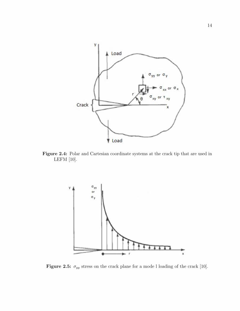
2.4 Polar and Cartesian coordinate systems at the crack tip that are used

in LEFM [10]. . . . . . . . . . . . . . . . . . . . . . . . . . . . . . . . 14

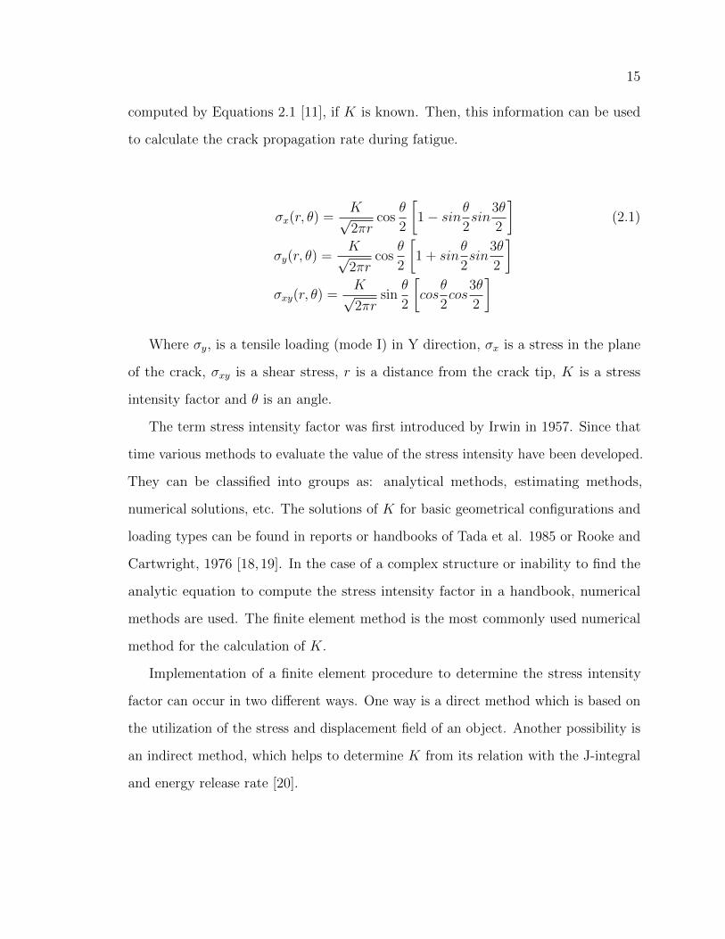
2.5 σyy stress on the crack plane for a mode l loading of the crack [10]. . . 14

2.6 Three stages of fatigue crack growth [27]. . . . . . . . . . . . . . . . . 18

2.7 Evaluation of the SIF from the the crack tip opening angle (CTOA) [38]. 23

3.1 Stress variation in a fatigue load cycle [41]. . . . . . . . . . . . . . . . 25

3.2 Typical S-N Curve [43]. . . . . . . . . . . . . . . . . . . . . . . . . . . 26

4.1 Two-dimensional model of the plate with following parameters: W =

0.1143 m, L = 0.1143 m, r = 0.003175 m. . . . . . . . . . . . . . . . . 29

4.2 Mesh used for FEA analysis. . . . . . . . . . . . . . . . . . . . . . . . 30

4.3 The result of the FEA stress analysis on a plate with a hole. . . . . . 31

4.4 a) Two-dimensional model of a plate with a hole and b) the result of

the material force vectors taken from the literature [46]. . . . . . . . . 32

4.5 Two-dimensional plate with a hole for FEA analysis . . . . . . . . . . 33

x

4.6 Material force vectors magnitude computed with VrSuite. . . . . . . . 33

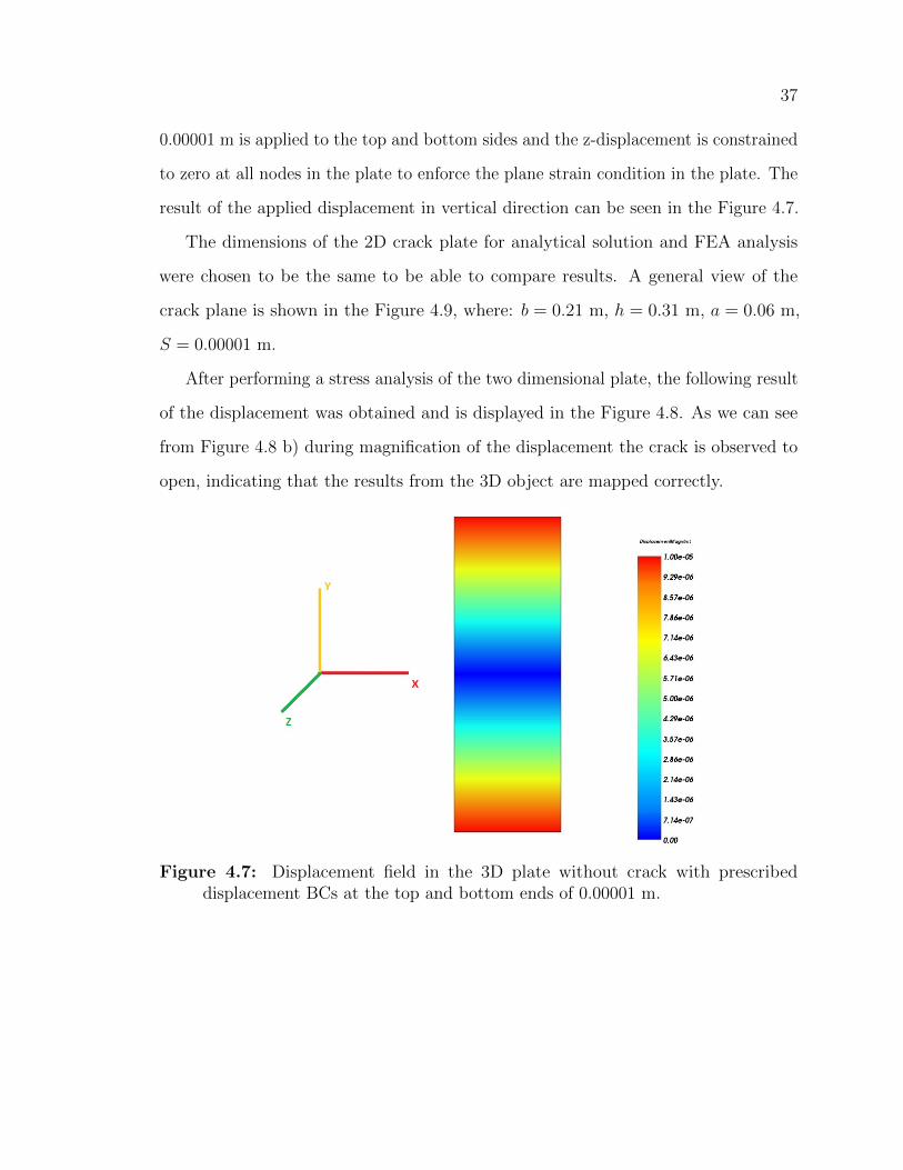
4.7 Displacement field in the 3D plate without crack with prescribed dis-

placement BCs at the top and bottom ends of 0.00001 m. . . . . . . . 37

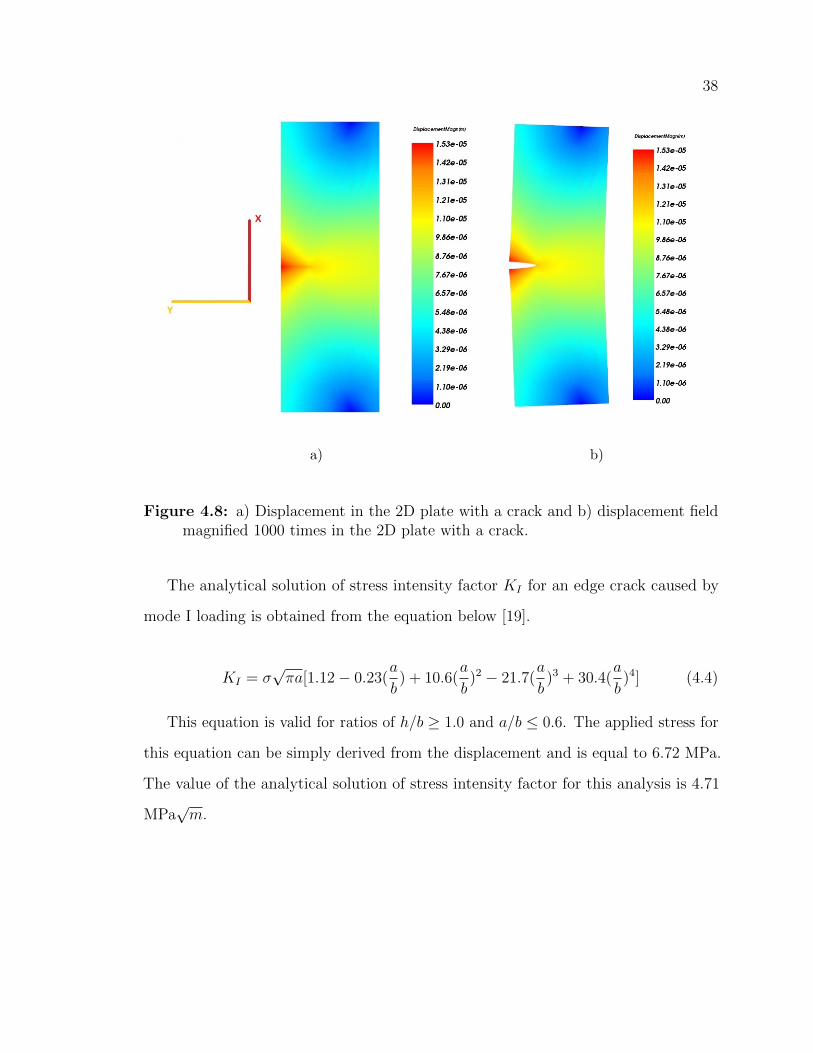
4.8 a) Displacement in the 2D plate with a crack and b) displacement field

magnified 1000 times in the 2D plate with a crack. . . . . . . . . . . . 38

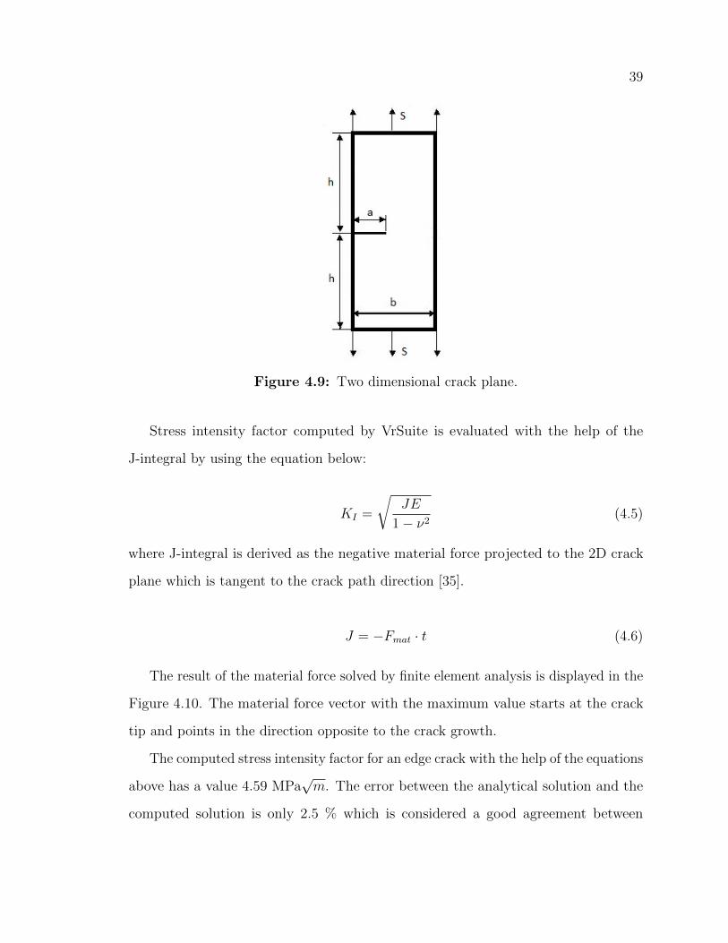
4.9 Two dimensional crack plane. . . . . . . . . . . . . . . . . . . . . . . 39

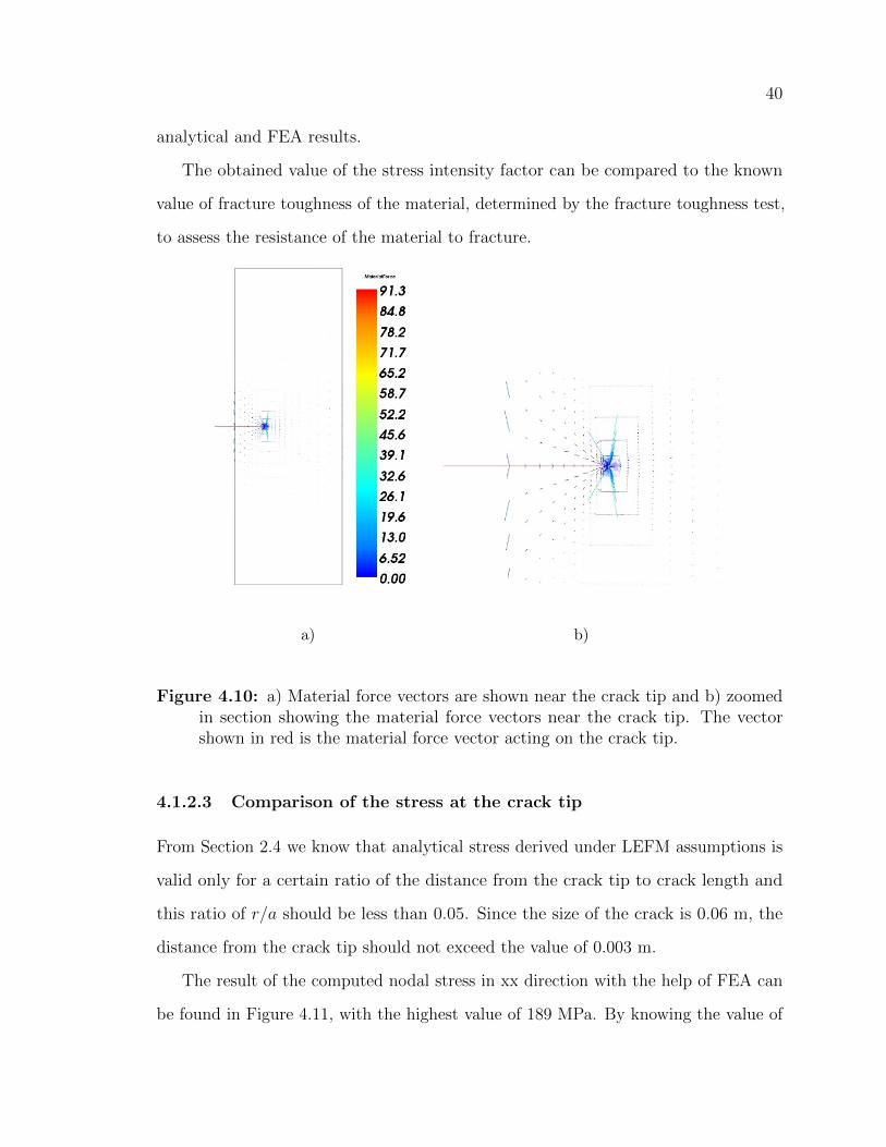
4.10 a) Material force vectors are shown near the crack tip and b) zoomed

in section showing the material force vectors near the crack tip. The

vector shown in red is the material force vector acting on the crack tip. 40

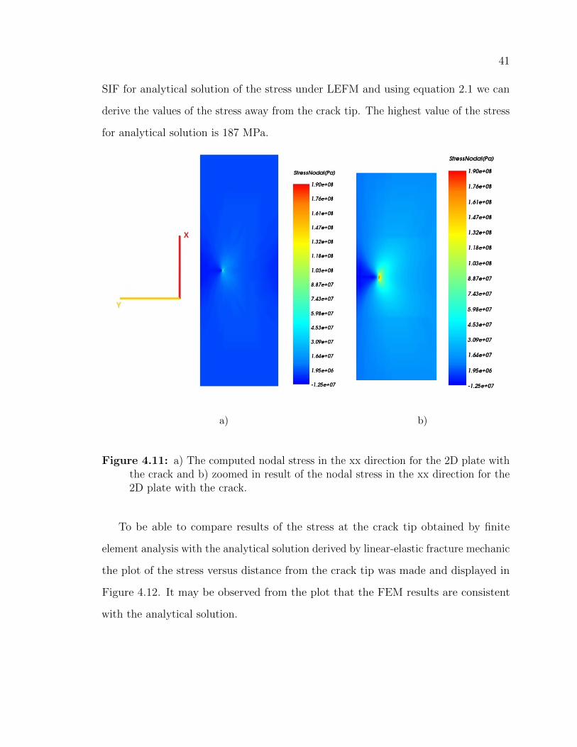
4.11 a) The computed nodal stress in the xx direction for the 2D plate with

the crack and b) zoomed in result of the nodal stress in the xx direction

for the 2D plate with the crack. . . . . . . . . . . . . . . . . . . . . . 41

4.12 Comparison of the stresses at the crack tip computed by FEA with

analytical solution derived by LEFM. . . . . . . . . . . . . . . . . . . 42

4.13 Geometry of the specimen. Triad axes: red is the X axis, yellow is the

Y axis, green is the Z axis. . . . . . . . . . . . . . . . . . . . . . . . . 44

4.14 a) Result of the Gauss points that show a principal stress in the

structure b) Zoomed in region of the Gauss points with narrow range

of the maximum values. . . . . . . . . . . . . . . . . . . . . . . . . . 45

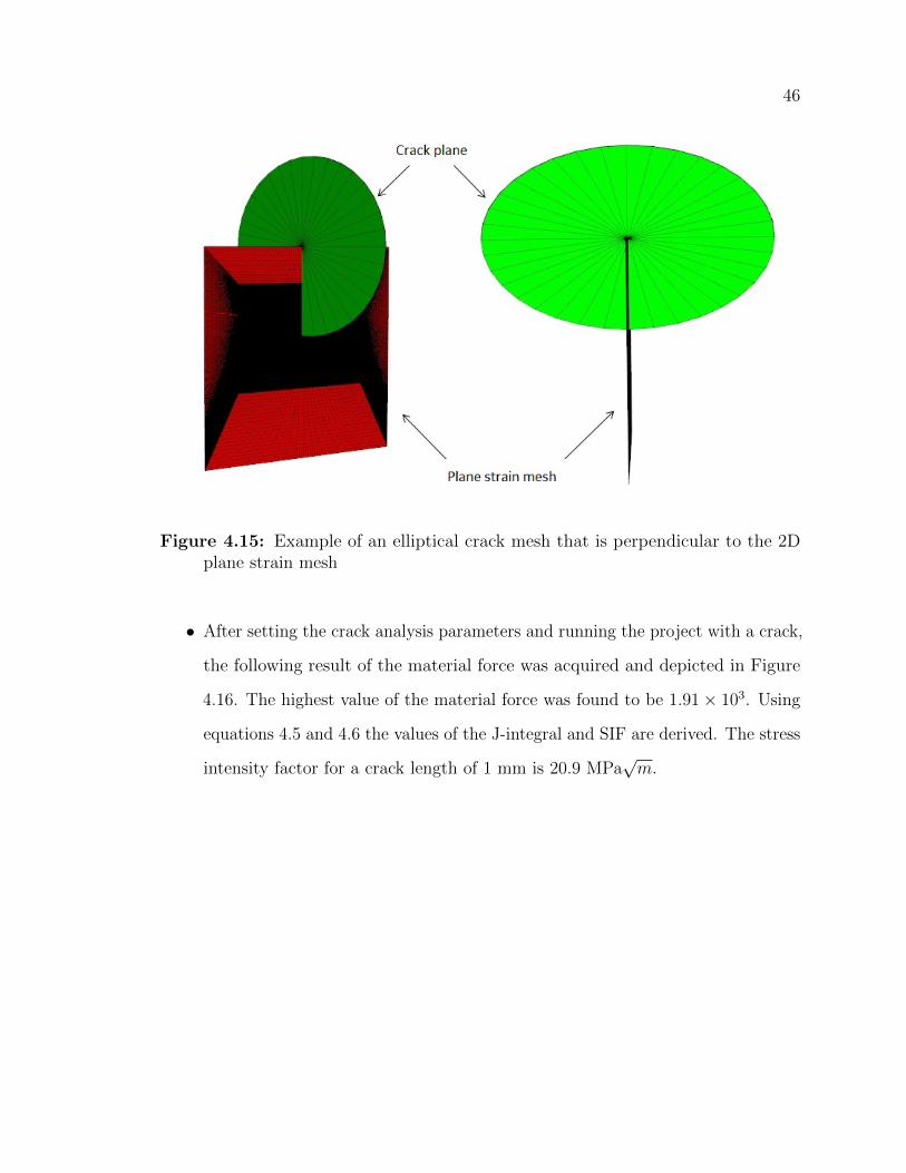
4.15 Example of an elliptical crack mesh that is perpendicular to the 2D

plane strain mesh . . . . . . . . . . . . . . . . . . . . . . . . . . . . . 46

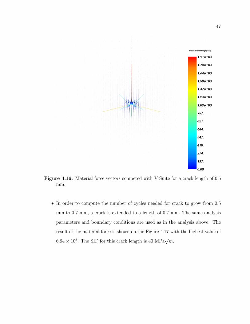
4.16 Material force vectors competed with VrSuite for a crack length of 0.5

mm. . . . . . . . . . . . . . . . . . . . . . . . . . . . . . . . . . . . . 47

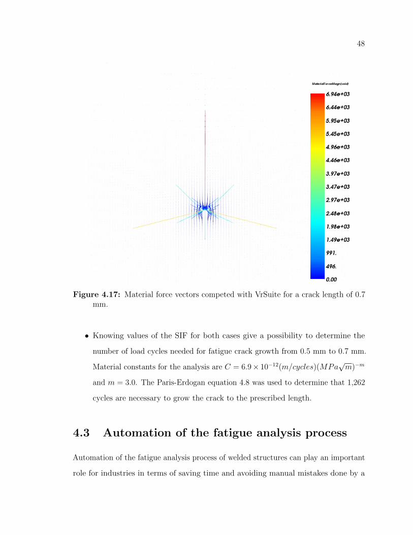
4.17 Material force vectors competed with VrSuite for a crack length of 0.7

mm. . . . . . . . . . . . . . . . . . . . . . . . . . . . . . . . . . . . . 48

4.18 First step of an automated crack wizard . . . . . . . . . . . . . . . . 52

4.19 Second step of an automated crack wizard . . . . . . . . . . . . . . . 53

xi

4.20 Third step of an automated crack wizard . . . . . . . . . . . . . . . . 54

4.21 Fourth step of an automated crack wizard . . . . . . . . . . . . . . . 55

4.22 Displacement at the crack tip of an analysis with an elastic material -

sharp crack and an analysis with an elastic-plastic material - blunting

crack. . . . . . . . . . . . . . . . . . . . . . . . . . . . . . . . . . . . 56

4.23 Geometry of the 3D object. . . . . . . . . . . . . . . . . . . . . . . . 57

4.24 a) Traction BC applied to the 3D object vs time step b) Displacement

vs time step for the 3D object. . . . . . . . . . . . . . . . . . . . . . . 57

4.25 Displacement vs Distance from the crack tip for the time step five

in Figure 4.24. See Figure 4.22 for a schematic of elastic and the

elastic-plastic displacement for given applied traction BC. . . . . . . . 58

4.26 The result of the crack tip blunting evolution is plotted vs the applied

stress for the load steps shown in Figure 4.24. . . . . . . . . . . . . . 60

4.27 a) Geometry of the WIC specimen with turned on mesh b) Cross-section

of the weld joint of the WIC specimen. . . . . . . . . . . . . . . . . . 61

4.28 a) a) Geometry of the pipe girth weld b) cross-section of the weld joint

of the pipe girth weld. . . . . . . . . . . . . . . . . . . . . . . . . . . 62

4.29 a) Location of the crack in the WIC test specimen b) An elliptical crack

mesh with perpendicular to it 2D crack plane in the WIC test specimen

with turned-off parts. . . . . . . . . . . . . . . . . . . . . . . . . . . . 63

4.30 a) Location of the crack in the pipe weld b) an elliptical crack mesh

shown in light green with the plane strain 2D mesh perpendicular to

the crack tip in the pipe girth weld. The pipe parts are made invisible

to show the crack and the plane strain 2D mesh. . . . . . . . . . . . . 64

A.1 The displacement field in a 2D plane strain mesh with a crack is shown. 74

A.2 The displacement field in a 2D plane strain mesh with a crack is shown.

Magnified 5 times. . . . . . . . . . . . . . . . . . . . . . . . . . . . . 75

xii

A.3 The xx stress is shown in a 2D plane strain mesh with a crack. . . . . 76

A.4 The computed material force vectors near the crack tip in a 2D plane

strain mesh. . . . . . . . . . . . . . . . . . . . . . . . . . . . . . . . . 77

A.5 Plot of the stress vs distance from the crack tip down in the plane of

the crack. . . . . . . . . . . . . . . . . . . . . . . . . . . . . . . . . . 78

A.6 Plot of the displacement vs distance from the crack tip to the distance

of one element in the crack opening direction. . . . . . . . . . . . . . 79

B.1 The displacement field in a 2D plane strain mesh with a crack is shown. 82

B.2 The displacement field in a 2D plane strain mesh with a crack is shown.

Magnified 5 times. . . . . . . . . . . . . . . . . . . . . . . . . . . . . 83

B.3 The xx stress is shown in a 2D plane strain mesh with a crack. . . . . 84

B.4 The computed material force vectors near the crack tip in a 2D plane

strain mesh. . . . . . . . . . . . . . . . . . . . . . . . . . . . . . . . . 85

B.5 Plot of the stress vs distance from the crack tip down in the plane of

the crack. . . . . . . . . . . . . . . . . . . . . . . . . . . . . . . . . . 86

B.6 Plot of the displacement vs distance from the crack tip to the distance

of one element in the crack opening direction. . . . . . . . . . . . . . 87

C.1 The displacement field in a 2D plane strain mesh with a crack is shown. 90

C.2 The displacement field in a 2D plane strain mesh with a crack is shown.

Magnified 5 times. . . . . . . . . . . . . . . . . . . . . . . . . . . . . 91

C.3 The xx stress is shown in a 2D plane strain mesh with a crack. . . . . 92

C.4 The computed material force vectors near the crack tip in a 2D plane

strain mesh. . . . . . . . . . . . . . . . . . . . . . . . . . . . . . . . . 93

C.5 Plot of the stress vs distance from the crack tip down in the plane of

the crack. . . . . . . . . . . . . . . . . . . . . . . . . . . . . . . . . . 94

C.6 Plot of the displacement vs distance from the crack tip to the distance

of one element in the crack opening direction. . . . . . . . . . . . . . 95

xiii

List of Acronyms

BC Boundary Condition

CTOA Crack Tip Opening Angle

CTOD Crack Tip Opening Displacement

EPFM Elastic Plastic Fracture Mechanics

FEA Finite Element Analysis

FEM Finite Element Method

GUI Graphical User Interface

LEFM Linear Elastic Fracture Mechanics

S-N Stress-Number of Cycles

SIF Stress Intensity Factor

WIC Welding Institute of Canada

xiv

Chapter 1

Introduction

1.1 Background

In the engineering world, the two most common and principal methods of joining

metal parts are welding and bolting. Considerations of aesthetic appearance as well as

the limited shear strength of bolts and resulting low endurance limit the application

of bolted joints in industry. In case of welding, the parts are joined together with

inter-atomic metallic bonds that ultimately form the weld joint. In many design

situations, welded joints are considered better than bolted ones because component

parts have nearly the same structural composition as the base material and the

strength is generally equal to or even higher than that of the constituent parts [1].

The critical area of a steel structure or a component is a welded joint. Material

properties at joints, such as ductility, ultimate strength, true stress vs strain relation-

ship, vary from one region to another around the weld. In fact, almost all failures of

welded structures occur because of the problems with welded joints. Failure depends

on the materials that are used, type of the environment and operating conditions.

The failure can be nucleated when the material approaches the limit of its strength,

which can cause fracture. The most common failure of welded structures is due to

fatigue which accounts for about 90% of failures [2]. Fatigue is a failure, which occurs

1

2

in structures when they are subjected to fluctuating and dynamic stresses less than

the yield stress of the material [3]. This type of failure can initiate at a stress level

considerably lower than the yield or tensile strength for a static load. Fatigue nucleates

cracks, that usually start at the surface. Once the crack is nucleated, it slowly grows

by the virtue of a repeated cyclic load. This leads to a progressive damage on a

reduced cross sectional area.

The loss of money or life when a structure fails due to fatigue failure can be large.

The necessity for research to improve the longevity and reliability of the welded joints

is therefore important. During the time of technical progress and computerization of

the world, the use of finite element method has played a large role in engineering. This

tool can help to assess the stresses caused by welding and in-service loading, as well as

estimate the fatigue life of the structure, prior to its actual failure. Another positive

side of computational weld mechanics for manufacturing is its time and money saving

aspect.

According to Jonsson (2011), ”Today, most programs, using finite element analysis

can easily calculate any stress field, but the stress intensity at the crack tip requires

more attention. Some programs can perform this type of analysis without putting

much effort, but when it approaches to the calculation of automatic crack growth, the

list of them narrows down only to a very few programs. It can be a complicated task

for three dimensional analysis, since the mesh around the growing crack has to be

remeshed for every step as well as moved in the right direction. To provide designers

with a tool for building optimised lightweight structures, a future trend would be

to build a software able to automatically calculate the crack path in a general three

dimensional structure without having to put a lot of work into the task, personal or

computational” [4].

3

1.2 Research Strategy

This thesis adopts the following research strategy.

1. An 3D transient non-linear analysis is done of welding a structure to compute

the final state after welding. Instead of welding, this analysis could be for any

manufacturing process that is capable of the computing the final state such as

deformation, microstructure and residual stress. Any solver that can output the

final state of the manufacturing process could be used.

2. Then, a 3D space-time analysis of a structure is done with in-service loads. The

initial state is the final state of the manufactured structure, system or component.

In this thesis, this is a quasi-steady state analysis of a welded structure with

in-service loads.

3. The first two analyses were macroscopic and assume the structure has no cracks.

The third analysis chooses locations that are considered to have a high risk of

cracks nucleating, growing and leading to failure. In this thesis, FEM Gauss

points with the highest values of principal tensile stress are considered to be

the points of highest risk. At chosen Gauss points considered to be high risk,

an elliptical crack is created that is normal to the principal tensile stress and

2D plane strain FEM meshes are created at points on the crack tip curve that

normal to the crack tip.

4. These plane strain FEM analyses of these 2D meshes are solved with boundary

tractions imported from the neighbourhood of this point in the second stress

analysis. The stress intensity is computed at the point that the 2D mesh

intersects the crack curve.

5. The number of load cycles to grow the fatigue crack a specified incremental

distance is computed by solving the Paris-Erdogan equation. Other rules to

4

choose the points of high risk of nucleating cracks could be used and other

attributes of the crack parameters such as length and width could be chosen.

6. In a design stage, this risk must be predicted and this strategy could be used

to optimize the design and reduce the risk of failure. In a structure operating

with in-service loads, the crack location and parameters might be observed from

NDT measurements. In this case, the observed data could be used to specify

the crack location, size, shape and this strategy could be used to estimate the

remaining life of the structure and to optimize the location and frequency of

NDT tests.

7. Each 2D plane strain problem solve takes less than a minute of CPU time to

solve with almost no effort to reduce CPU time. The solves are independent

and thus trivially parallelizable. It is likely that CPU time could be reduced

significantly. Parallel processing could be used to solve 1000’s of potential crack

locations for a given structure with given in-service loads.

One of the goals of this thesis is to demonstrate the capability to automate this

procedure to minimize user time and user expertise in setting up the analyses and

generating final reports.

1.3 Directional scope of this study

By investigation of works performed by other researchers, in the scope of fatigue

analysis, it was feasible to notice potential expansions of scope and new areas of study

that will be presented in this thesis. Some of the works will be described here.

Pyttel B., SchwerdtD., et al. [5] provides an overview of the current research on

high cyclic fatigue failure (Nf > 107). The study provides a list of test facilities

that are used for the research. Materials with typical S-N curves and affecting

5

factors like residual stresses and notches are stated. The research tries to explain

distinct failure mechanisms which occur while testing of the specimens. A double

S-N curve is recommended for the representation of the fatigue behaviour, to take

into account different failure mechanisms. One of the curves describes the surface

fatigue strength behaviour and another one describes the volume fatigue strength

behaviour. Recommendations about fatigue design of parts are given. Future scope

of work about fatigue assessment of polymer components that are subjected to high

number of loading cycles is established.

Myung Hyun Kima, Seong Min Kima, et al. [6] reveals a study of a fatigue strength

assessment with the help of the hot spot stress method and the structural stress method,

performed for a side shell connection of a container vessel. The study describes an

approach for calculating the extrapolated hot spot stress for design purposes built

on converged hot spot stresses. As a result, with the help of these two methods, hot

spot stress approach and structural stress approach the fatigue strength at hot spot

locations of a typical ship structure is predicted and compared. As a conclusion, it

is mentioned that structural stress approach can be used as a viable alternative for

the fatigue strength assessment of offshore structures and ships. Further directions of

investigation related to fatigue strength of offshore structures are proposed.

Tveiten B. W. & Moan T. [7] reviews the existing hot-spot stress methodology for

plate structures; develops and verifies general and modern method for the structural

stress extrapolation that can be used along with a hot-spot design S-N curve for

ship structures made of aluminium. The research of Tveiten is intended to refine the

analysis methodology built on the calculation of the structural stress and the selection

of the appropriate S-N curves. The proposed method is used for determining the

optimum location of points for stress extrapolation based on the asymptotic behaviour

of the stresses adjacent to an idealized notch. Description of test rigs which were used

for fatigue test is given. From the results of fatigue tests obtained in this research,

6

appropriate S-N curves along with a proposed extrapolation procedure can be used as

a suitable choice for determining the structural stress and the fatigue assessment.

Maddox S. J. [8] gives a revision of methods, codes and standards related to

the fatigue assessment of welded aluminium structures. Methods assessment for

fatigue analysis of welded aluminium structures is made based on an estimation of the

residual life of existing structures. Assessment of the methods includes information

obtained from a literature search, but is primarily referenced to data used in recent

fatigue design standards. Close attention is paid to recent fatigue data, acquired from

structural components representative of actual structures. The research states that

among the described fatigue assessment methods, the use of the nominal stress S-N

curves is the most standardized and developed. The author assumes that in future

the hot-spot stress approach will probably be the most valuable approach used for

structural design.

Poutiainen I. & Marquis G. [9] presents a method that is intended to expand

the feasibility of structural stress method for fatigue analysis in welded structures.

Conventional methods used for fatigue assessment are not able to take into account

the effect of the weld size. Current study suggests a linearization of the local stress

distribution through the thickness of the part in the plane of the weld toe, so the stress

distribution is dependent on the size of the weld, part thickness and applied load. The

paper covers equations used for calculating of the bilinear stress distribution. It is

mentioned that the method was applied only to fully load-carrying welds, however

it can also be used for partial load-carrying welds. The proposed stress distribution

can be treated as a modification of the structural stress and it can be used in the

same way as the conventional structural stress in the fatigue assessment of the welded

structures.

7

1.4 Objectives

This work is an attempt to evaluate the possibility and applicability of finite element

method for fatigue analysis and crack growth prediction of welded structures. The

aim of using the finite element method in fatigue analysis and design is to obtain a

more precise estimation of the loads and stresses produced in the welded structures

due to the welding process and in-service loadings. The fatigue analysis will be

performed using VrSuite Software. VrSuite Software is a finite element analysis

package, which can simulate welding processes, microstructural analysis and heat

treatment. Different test cases composed of various geometries, meshes and materials

are computed using VrSuite package to estimate the stress concentration and the stress

intensity factors. Ultimately, the results of the stress intensity factor, computed by the

finite element method, are compared to an analytical solutions used in linear-elastic

fracture mechanics.

1.5 Scope and Organization of the Thesis

This thesis is divided into five chapters. Chapter 1 is an introduction to the thesis.

It lists fatigue analysis studies that were conducted by other researchers. The basic

understanding of factors that lead author to choose this topic, the general concept of

the thesis, the outline of the research and objectives were also given in the Chapter

1. Chapter 2 gives insight into fracture mechanics theory, stress intensity factor

calculation, crack initiation and propagation processes. Chapter 3 summarizes the

theory used for fatigue life prediction which includes the fatigue analysis assessment

methods. Chapter 4 includes the problem geometry definition and set-up, the analysis

of the test cases based on the criteria of the stress concentration factor, the verification

of the VrSuite by comparing results obtained from the FEA with an analytical solutions

8

and discussion of the obtained results. The conclusion and recommendations for the

future work directions are given in Chapter 5.

Chapter 2

Fracture mechanics theory

2.1 Fracture mechanics concept

Since cracks cannot be entirely eliminated, and they can lower the strength of a product

below its expected strength, it is crucial to have the capability to quantify and predict

the lifetime of a cracked structure under service load conditions. Fracture mechanics

is the primary tool to analyse fatigue failures and brittle fracture in components.

The main principle of the fracture mechanics is to provide a method of assessing

the maximum service loading condition the component with a given crack size can

withstand. Fracture mechanics is used to provide information on the conditions that

lead a particular structure to failure and can also be used as a preventive measure for

the life assessment of future products that operate in the same conditions. Fracture

mechanics depend upon material properties, stresses induced by applied loads, defect

size, shape and location. The behaviour of cracks in fracture mechanics is based on

a stress analysis in the vicinity of the crack. Depending on the plastic region in the

vicinity of the crack tip, fracture mechanics can be divided into linear elastic fracture

mechanics (LEFM) and elastic plastic fracture mechanics (EPFM).

LEFM is associated with a small amount of plastic deformation at the vicinity of

the crack tip. The parameter, which characterizes behaviour of the crack in linear

9

10

elastic fracture mechanics, is defined by the value of the stress intensity factor (K).

Structures, used for LEFM evaluation require a high level of tensile strength along

with a relatively low level of fracture toughness. In turn, elastic plastic fracture

mechanics is used in cases when the plastic zone at the crack tip is slightly more

extensive. EPFM is commonly used for the lower-strength structures with higher level

of fracture toughness [10].

2.2 Linear elastic fracture mechanics

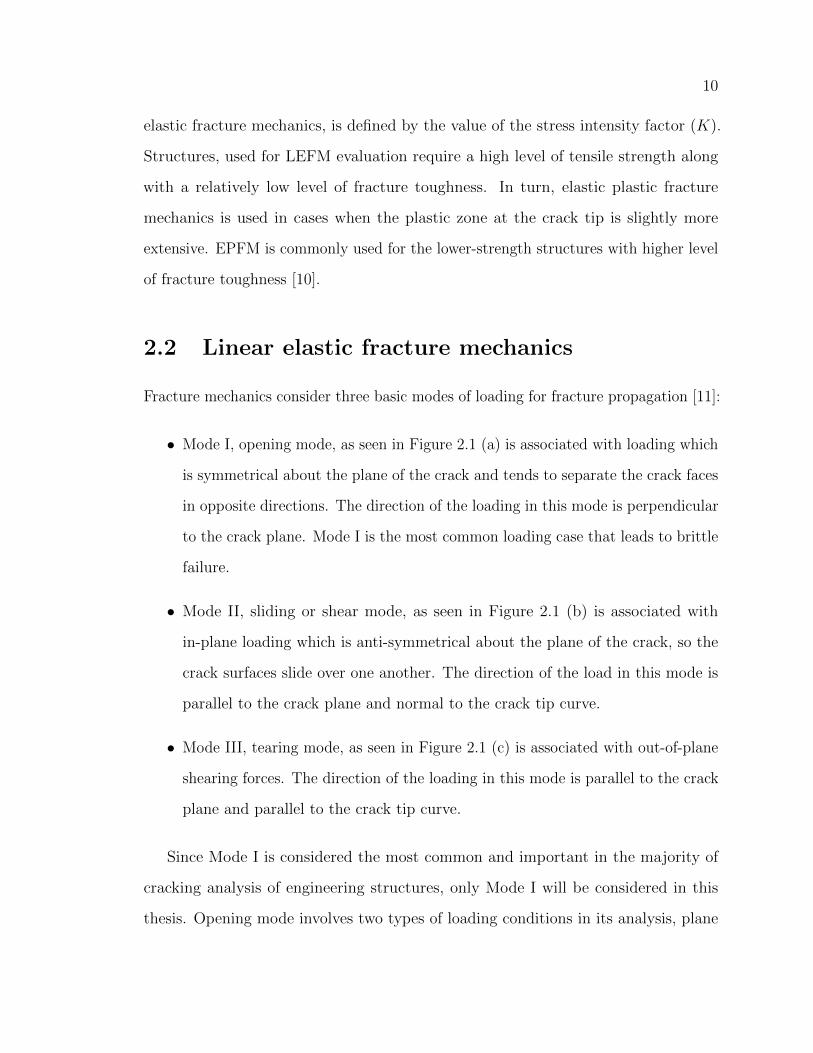
Fracture mechanics consider three basic modes of loading for fracture propagation [11]:

• Mode I, opening mode, as seen in Figure 2.1 (a) is associated with loading which

is symmetrical about the plane of the crack and tends to separate the crack faces

in opposite directions. The direction of the loading in this mode is perpendicular

to the crack plane. Mode I is the most common loading case that leads to brittle

failure.

• Mode II, sliding or shear mode, as seen in Figure 2.1 (b) is associated with

in-plane loading which is anti-symmetrical about the plane of the crack, so the

crack surfaces slide over one another. The direction of the load in this mode is

parallel to the crack plane and normal to the crack tip curve.

• Mode III, tearing mode, as seen in Figure 2.1 (c) is associated with out-of-plane

shearing forces. The direction of the loading in this mode is parallel to the crack

plane and parallel to the crack tip curve.

Since Mode I is considered the most common and important in the majority of

cracking analysis of engineering structures, only Mode I will be considered in this

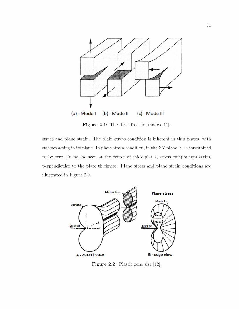
thesis. Opening mode involves two types of loading conditions in its analysis, plane

11

Figure 2.1: The three fracture modes [11].

stress and plane strain. The plain stress condition is inherent in thin plates, with

stresses acting in its plane. In plane strain condition, in the XY plane, εz is constrained

to be zero. It can be seen at the center of thick plates, stress components acting

perpendicular to the plate thickness. Plane stress and plane strain conditions are

illustrated in Figure 2.2.

Figure 2.2: Plastic zone size [12].

12

2.3 Crack initiation

Crack initiation in metals can be considered as the formation of a void due to irreversible

motion of dislocations under repeated deformation. The mechanism of void initiation

in a ductile material can be characterized as homogeneous or heterogeneous. In

case of a homogeneous crack nucleation, the voids initiate through the process of

vacancy mitigation and dislocation interactions. In turn, the main characteristic of

heterogeneous nucleation is interaction between dislocations and inclusions or other

structural discontinuities [13]. Fatigue crack growth is usually slow and in many cases

can be predicted by the use of fracture mechanics. Linear elastic fracture mechanics

assumes quasi-static behaviour of the crack growth and a small plastic zone region in

the vicinity of the crack tip.

2.4 Crack tip plastic zone

An important parameter that has to be taken into consideration while using linear

elastic fracture mechanics is that the plastic zone at the crack tip must be small

relative to the crack length and other size parameters of the part. Irwin noticed that if

the size of the plastic zone is small compared to the size of the crack, then the amount

of the energy for crack initiation can be computed from the elastic solution [14]. At

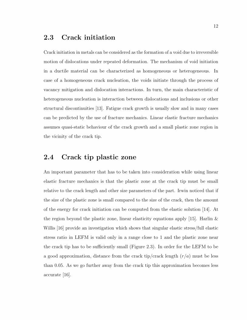
the region beyond the plastic zone, linear elasticity equations apply [15]. Harlin &

Willis [16] provide an investigation which shows that singular elastic stress/full elastic

stress ratio in LEFM is valid only in a range close to 1 and the plastic zone near

the crack tip has to be sufficiently small (Figure 2.3). In order for the LEFM to be

a good approximation, distance from the crack tip/crack length (r/a) must be less

than 0.05. As we go further away from the crack tip this approximation becomes less

accurate [16].

13

Figure 2.3: Plots of ratios of asymptotic forms to full stresses, as functions of r/a,adjacent to the tip of a buried crack in an elastic body, subjected to tensile stress.Where σ22 at θ = 0 corresponds to the tensile stress normal to the crack [16].

2.5 Stress intensity factor

During operational conditions of welded structures, macroscopic flaws can be formed

in a structure. Each of these flaws can be described as an infinitely sharp notch.

In LEFM the measure of the crack propagation can be characterized by a single

parameter called the stress intensity factor K. It characterizes the stress state in a

sufficiently small region in front of the crack tip caused by residual or remote stresses

and is illustrated in Figure 2.4. The value of this parameter depends on the crack size,

loading condition, the geometrical configuration of a crack and construction where the

crack is embedded [17]. The relationship between the stress state and the distance

from the crack tip is shown in Figure 2.5.

When the value of the stress intensity factor K reaches the value of the fracture

toughness, KC/IC , fracture in a structure will occur. The fracture toughness depends

on the thickness of the specimen.

The stress intensity factor describes the crack tip state. Components of the strain,

stress and displacement as a function of r and θ in the vicinity of the crack tip can be

14

Figure 2.4: Polar and Cartesian coordinate systems at the crack tip that are used inLEFM [10].

Figure 2.5: σyy stress on the crack plane for a mode l loading of the crack [10].

15

computed by Equations 2.1 [11], if K is known. Then, this information can be used

to calculate the crack propagation rate during fatigue.

σx(r, θ) =K√2πr

cosθ

2

[1− sinθ

2sin

3θ

2

](2.1)

σy(r, θ) =K√2πr

cosθ

2

[1 + sin

θ

2sin

3θ

2

]σxy(r, θ) =

K√2πr

sinθ

2

[cos

θ

2cos

3θ

2

]

Where σy, is a tensile loading (mode I) in Y direction, σx is a stress in the plane

of the crack, σxy is a shear stress, r is a distance from the crack tip, K is a stress

intensity factor and θ is an angle.

The term stress intensity factor was first introduced by Irwin in 1957. Since that

time various methods to evaluate the value of the stress intensity have been developed.

They can be classified into groups as: analytical methods, estimating methods,

numerical solutions, etc. The solutions of K for basic geometrical configurations and

loading types can be found in reports or handbooks of Tada et al. 1985 or Rooke and

Cartwright, 1976 [18,19]. In the case of a complex structure or inability to find the

analytic equation to compute the stress intensity factor in a handbook, numerical

methods are used. The finite element method is the most commonly used numerical

method for the calculation of K.

Implementation of a finite element procedure to determine the stress intensity

factor can occur in two different ways. One way is a direct method which is based on

the utilization of the stress and displacement field of an object. Another possibility is

an indirect method, which helps to determine K from its relation with the J-integral

and energy release rate [20].

16

2.6 Crack propagation and Paris-Erdogan equa-

tion

Cracks in isotropic material usually start to form in the opening mode and tend to

propagate in the direction perpendicular to the maximum tensile stress [21–23]. One of

the crucial parts of fracture mechanics approach is calculation of remaining component

life through prediction of the crack growth rate. The most common method which

is used for prediction of fatigue crack propagation is the Paris-Erdogan law. It was

long known that the rate of the crack propagation is not constant with time and

increases with larger stress amplitudes and larger cracks [24]. Paris et al. (1961)

was the first who proposed to use the stress intensity factor, developed by Irwin, for

characterization of the rate of crack growth per load cycle [25]. He pointed out that

fatigue crack growth increment per cycle relates to the increment in stress intensity

factor. The Paris-Erdogan equation has the following form:

da

dN= C(∆K)m (2.2)

The left side of the equation represents the crack growth per load cycle. It defines

the relation between the increment in the crack length with the number of load

cycles [24]. Where, a is the length of the crack, N is the number of load cycles, C

and m are material constants, ∆K is the increment in stress intensity factor in a load

cycle, that is expressed by the following equation:

∆K = Kmax −Kmin (2.3)

Where Kmax corresponds to the maximum value of stress intensity factor and Kmin

corresponds to the minimum value of the stress intensity factor in a load cycle.

In case of a known stress intensity factor, it is feasible to evaluate the fatigue crack

17

growth in any crack configuration by using the Equation 2.2.

The behaviour of fatigue crack propagation in metals can be assessed by the

increment in stress intensity factor per load cycle ∆K [26].

Paris-Erdogan equation is limited to:

1. Large enough crack size.

2. Small enough plastic zone compared to the size of the crack.

3. Constant amplitude load cycles

Generally, the rate of fatigue crack propagation can be divided into three distinct

regions as illustrated in Figure 2.6. In region I, where a threshold value of stress

intensity factor range is low, propagation of the crack usually is considered not to

occur under load fluctuation. This region is characterised by the small scale yielding

and a small plastic zone. Region II is characterized by the linear relation between a

crack growth rate and an increment in the stress intensity factor per load cycle. Crack

length in this region is large relative to the plastic zone size. Most of the concepts

that describe fatigue crack propagation behaviour in linear elastic fracture mechanics

are dealing with Region II. The Paris-Erdogan equation (Equation 2.2) is used to

represent this region. Region III is characterized by high and unstable fatigue crack

growth per cycle. The rate of the fatigue crack growth accelerates until the final

failure occurs [26].

2.7 Energy release rate

The process of crack formation and propagation involves conversion of energy [28].

Griffith was first to see the importance of energy variation during crack growth

in brittle solids [29]. He assumed that solids have a surface energy that must be

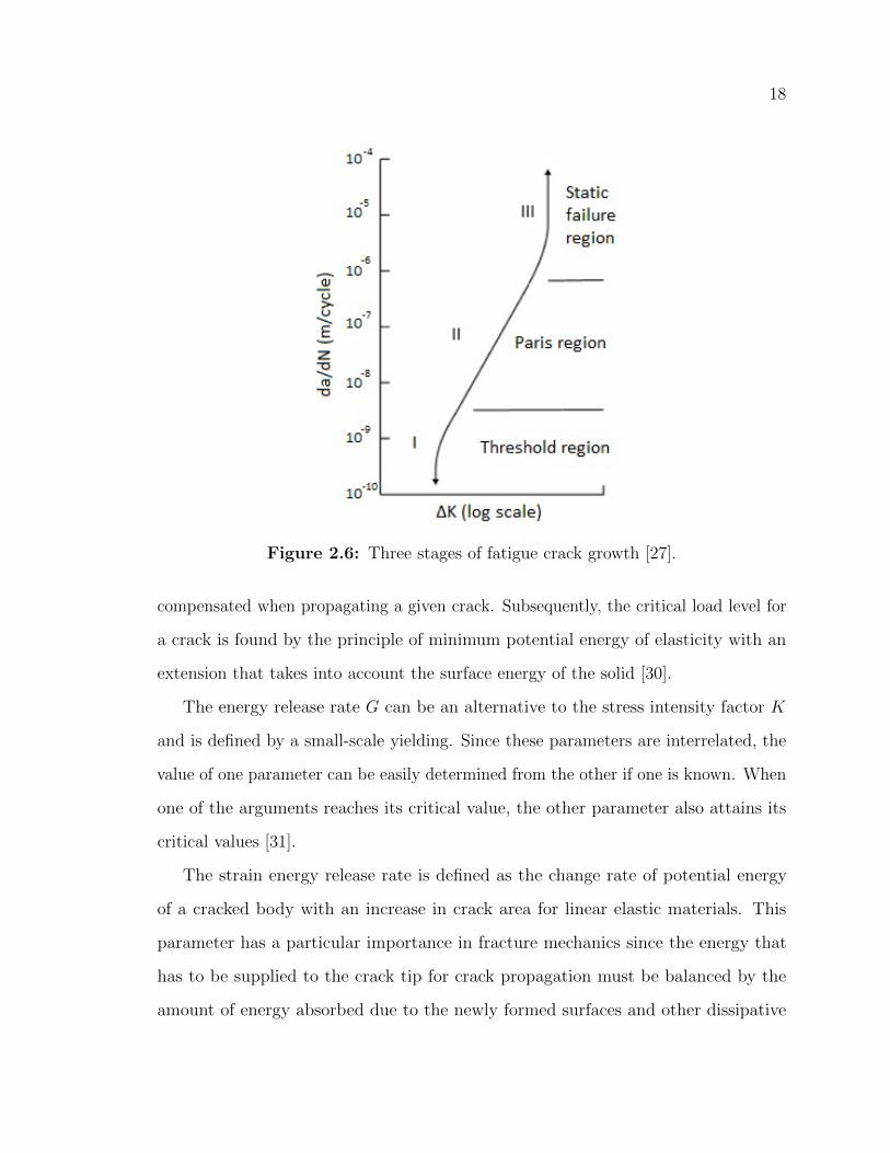
18

Figure 2.6: Three stages of fatigue crack growth [27].

compensated when propagating a given crack. Subsequently, the critical load level for

a crack is found by the principle of minimum potential energy of elasticity with an

extension that takes into account the surface energy of the solid [30].

The energy release rate G can be an alternative to the stress intensity factor K

and is defined by a small-scale yielding. Since these parameters are interrelated, the

value of one parameter can be easily determined from the other if one is known. When

one of the arguments reaches its critical value, the other parameter also attains its

critical values [31].

The strain energy release rate is defined as the change rate of potential energy

of a cracked body with an increase in crack area for linear elastic materials. This

parameter has a particular importance in fracture mechanics since the energy that

has to be supplied to the crack tip for crack propagation must be balanced by the

amount of energy absorbed due to the newly formed surfaces and other dissipative

19

processes such as plasticity [31]. Energy release rate can be defined as:

G = −dUdA

(2.4)

where, U is the potential energy available for crack growth, and A is the cracked

area. The energy release rate failure criterion says that a crack will continue to

propagate when the available G is equal to or greater than a critical value of energy

release rate Gc.

G ≥ Gc (2.5)

The value Gc is a brittle fracture energy that is considered to be a material property

and is independent of the applied loads and the body geometry [32].

In fracture mechanics J-integral and G energy release rate are energy based

parameters and directly related to stress intensity factor. Having either J-integral

or energy release rate can significantly help in defining the K. Irwin established the

following relation between fracture toughness and energy release rate [14]:

G =K2

IC

H(2.6)

where H is the general elastic modulus:

H = E (Plane stress) (2.7)

H =E

1− ν2(Plane strain) (2.8)

where E is a Modulus of Elasticity, and ν is the Poison’s ratio.

20

2.8 Material force method

The material force method is an essential feature for improving and verifying numerical

results computed with the Finite Element software. This concept provides clear and

physically proved parameters for fracture assessment and prediction of crack growth.

The method is based on the works of Eshelby [33] who used it to describe forces that

act on inhomogeneities and defects.

Fracture occurs when the crack driving force becomes sufficiently large and attains

the material’s fracture toughness value. Direction of the crack is opposite to the crack

driving force at the crack tip. Material force always appears at different types of

inclusions such as cracks, holes and slits in the structures. In case of FEA it will

appear at constrained nodes and boundary nodes [34].

In case of elasto-plastic and linear elastic material, material force and J-integral are

equivalent to the energy release rate. J-integral can be simply derived as a negative

material force projected on the 2D crack plane in the tangent to the crack path

direction t [35].

J = −Fmat · t (2.9)

Additional background on the theory of material forces is provided by the following

quotation from Steinmann [36].

The behavior of most materials (including composites, polycrystals,

granular media and soft tissues to name but a few) is known to be influenced

or even to be determined by inhomogeneities which those continua exhibit

at a microscopic level. In the past decades, considerable effort has thus been

concentrated on the development of extended continuum theories which are

designed to account for inherent microstructure in natural and engineering

materials. Existing extended continuum theories include among others

21

micromorphic and micropolar theories, generalized continuum formulations

based on order parameters and higher gradient formulations in either

internal variables, state variables or both. These approaches have, despite

their generally disparate nature, one thing in common: they are based on

what is known as the ”spatial setting” of continuum mechanics (alternatively

referred to as a ”direct-motion based formulation”).

However, it is also possible to take a different approach to the mod-

eling of microstructured continua suggested in essence in the mid-1950s

by Eshelby [37]: a material setting based continuum description which

gives rise to driving forces resulting from the material rearrangement of

inhomogeneities during the deformation of a solid-like continuum. These

driving forces essentially represent the tendency of general material defects

such as cracks, inclusions, phase boundaries, dislocations and the like to

move relative to the ambient material and are hence called material forces

or configurational forces. As such, they are complementing Newtonian

forces (regarded as physical driving forces for positional changes relative to

the ambient space) arising in the spatial setting. Material forces contribute

to the so-called balance of pseudomomentum, where they are balanced with

Eshelby’s stress tensor and the vector of pseudomomentum.

Examples of material forces are the PeachKoehler force acting on a

dislocation in a defective crystal, and, in the context of elastic fracture

mechanics, a vector-valued generalization of the classical J-integral, inte-

grating the normal projection of the Eshelby stress over a surface enclosing

the crack tip, namely

J = lim∂V r

0→0

∫∂V r

0

∑·Nda0 (2.10)

22

Here,∑

is the Eshelby stress tensor and N is the outward unit normal

vector on the regular part of the boundary, ∂V r0 .

The numerical analysis of material setting based continuum theories

has become known as the material force method. An appealing feature

of the latter is a straightforward and computationally cheap algorithmic

determination of the material forces: it reduces to a post-processing step

performed after the solution of the spatial motion problem has been deter-

mined and requires no additional data structures in addition to the usual

finite element structures.

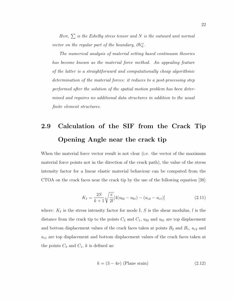
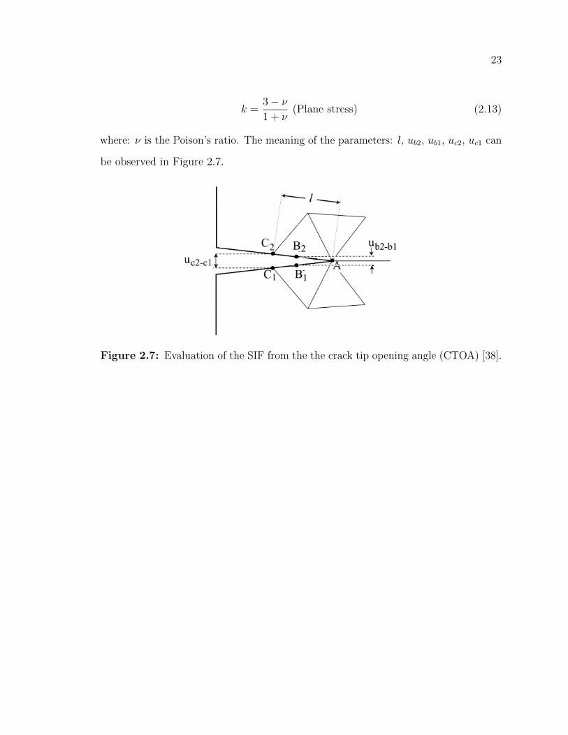
2.9 Calculation of the SIF from the Crack Tip

Opening Angle near the crack tip

When the material force vector result is not clear (i.e. the vector of the maximum

material force points not in the direction of the crack path), the value of the stress

intensity factor for a linear elastic material behaviour can be computed from the

CTOA on the crack faces near the crack tip by the use of the following equation [38]:

KI =2S

k + 1

√π

2l[4(ub2 − ub1)− (uc2 − uc1)] (2.11)

where: KI is the stress intensity factor for mode I, S is the shear modulus, l is the

distance from the crack tip to the points C2 and C1, ub2 and ub1 are top displacement

and bottom displacement values of the crack faces taken at points B2 and B1, uc2 and

uc1 are top displacement and bottom displacement values of the crack faces taken at

the points C2 and C1, k is defined as:

k = (3− 4ν) (Plane srain) (2.12)

23

k =3− ν1 + ν

(Plane stress) (2.13)

where: ν is the Poison’s ratio. The meaning of the parameters: l, ub2, ub1, uc2, uc1 can

be observed in Figure 2.7.

Figure 2.7: Evaluation of the SIF from the the crack tip opening angle (CTOA) [38].

Chapter 3

Fatigue analysis assessment methods

3.1 Introduction

Fatigue is a failure mechanism which occurs due to the action of dynamic and

fluctuating stresses that lead to loss of the structure’s nominal strength. Fatigue

analysis of welded structures is of a high practical interest for cyclic loaded engineering

structures such as bridges, cranes, vehicles, ships, offshore structures, etc. Fatigue

in welded structures is a complicated process. Fatigue failures in welded structures

mostly appear at the welds rather than in the base metal, even though the base metal

may contain preliminary notches or cracks. The effects of the heating process and

subsequent cooling of the weld as well as the fusion process create high residual stress

concentrations in the weld with different geometrical parameters. Furthermore, welds

usually contain cavities, pores, inclusions, undercuts, etc which act as stress raisers.

A parameter that affects the fatigue behaviour of a weld joint is the residual stress

and the distortion due to the welding process [39].

Fatigue failure always occurs at a stress level less than the tensile or yield strength

for a static load. When the number of load cycles for a given level of stress intensity

exceeds some tolerance threshold, microscopic cracks will initiate at the surface of the

structure. Material damage starts in the crystalline structure and grows slowly by

24

25

the cyclic plastic deformation as the stress cycles are repeated [40]. When the crack

reaches a critical size due to fatigue the structure will suddenly fail.

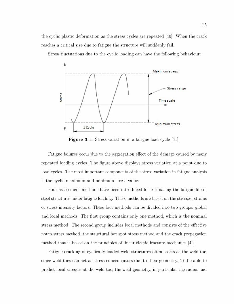
Stress fluctuations due to the cyclic loading can have the following behaviour:

Figure 3.1: Stress variation in a fatigue load cycle [41].

Fatigue failures occur due to the aggregation effect of the damage caused by many

repeated loading cycles. The figure above displays stress variation at a point due to

load cycles. The most important components of the stress variation in fatigue analysis

is the cyclic maximum and minimum stress value.

Four assessment methods have been introduced for estimating the fatigue life of

steel structures under fatigue loading. These methods are based on the stresses, strains

or stress intensity factors. These four methods can be divided into two groups: global

and local methods. The first group contains only one method, which is the nominal

stress method. The second group includes local methods and consists of the effective

notch stress method, the structural hot spot stress method and the crack propagation

method that is based on the principles of linear elastic fracture mechanics [42].

Fatigue cracking of cyclically loaded weld structures often starts at the weld toe,

since weld toes can act as stress concentrators due to their geometry. To be able to

predict local stresses at the weld toe, the weld geometry, in particular the radius and

26

angle of a toe must be taken into account.

3.2 Properties of S-N curve

Generally, fatigue assessment tests can be divided into two types. The first type

focuses on the nominal stress which cause fatigue failures for a definite number of

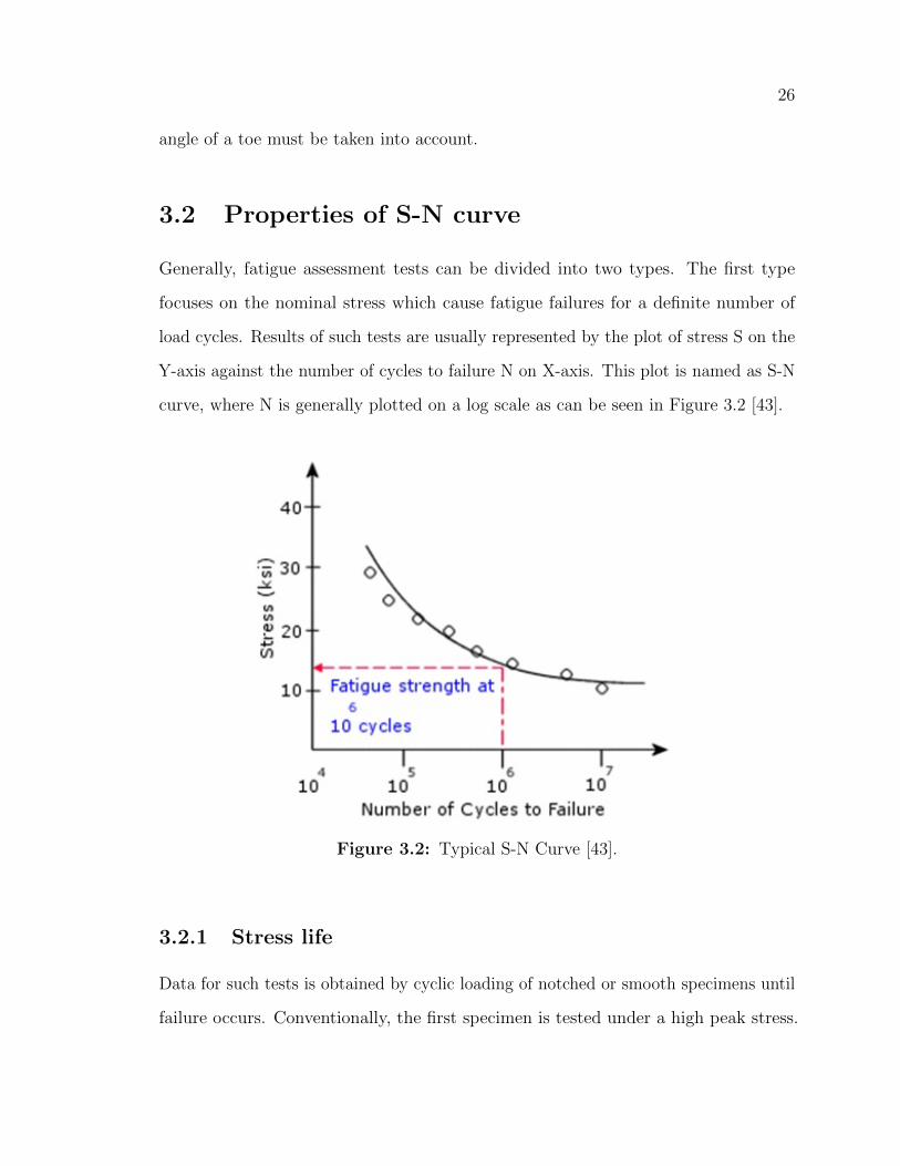
load cycles. Results of such tests are usually represented by the plot of stress S on the

Y-axis against the number of cycles to failure N on X-axis. This plot is named as S-N

curve, where N is generally plotted on a log scale as can be seen in Figure 3.2 [43].

Figure 3.2: Typical S-N Curve [43].

3.2.1 Stress life

Data for such tests is obtained by cyclic loading of notched or smooth specimens until

failure occurs. Conventionally, the first specimen is tested under a high peak stress.

27

Further tests are performed with decreasing levels of stress until the specimens do not

fail in a given number of cycles. Usually the maximum number of cycles are equal to

107. Fatigue threshold stress is determined as the maximum stress at which run-out

appears [44].

3.2.2 Strain life

Another type of fatigue test is the cyclic strain controlled test. While operating this

test the strain amplitude is kept constant during the cyclic loading. This type of

test is more typical for loading found during thermal cycling, wherein the specimen

contracts and expands due to oscillation in the operating temperature [43].

Chapter 4

Finite element analysis

4.1 Problem analysis

4.1.1 Two-dimensional stress analysis of a plate with a hole

The following analysis evaluates accuracy and correspondence of the stress state of

two-dimensional objects done by a finite element analysis with analytical solutions.

The plate has a central hole and is subjected to tensile loading. The current analysis:

- Compares the maximum stress in the structure to the one derived from the

analytical solution.

- Compares the calculated direction and magnitude of the material force vector to

the one obtained from the literature.

4.1.1.1 Determination of the maximum stress

The analysis consists of a two dimensional plate with a hole in its center. Material

that is used for this analysis is BABAnderson steel. The mesh type is 4 node quads.

A tensile load is applied to the opposite sides of the plate. The plate has the following

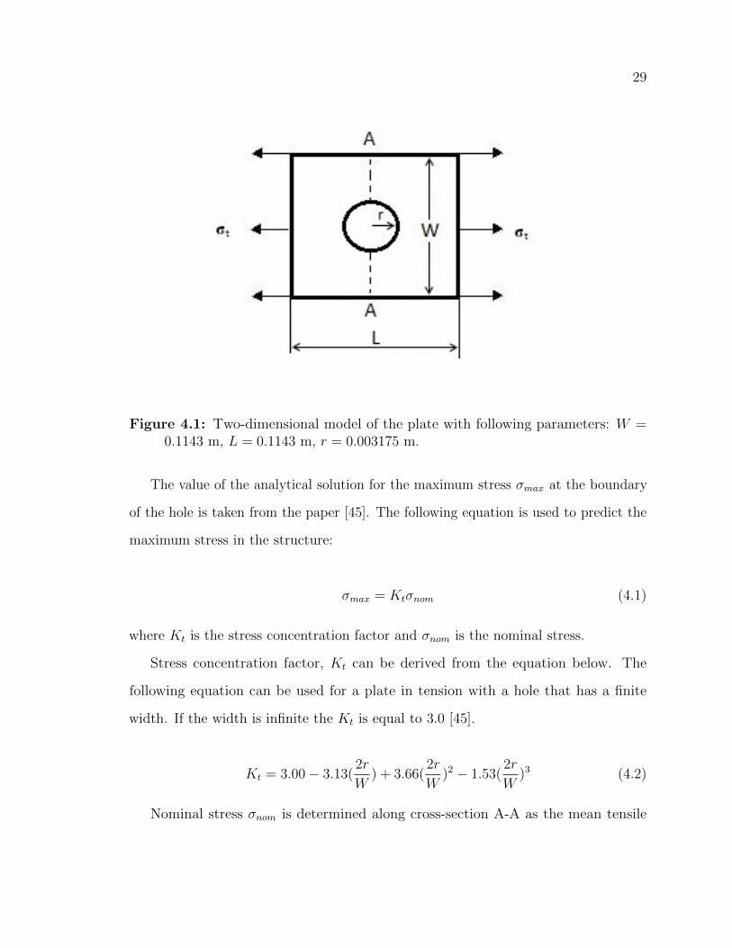
parameters: W = 0.1143 m, r = 0.003175 m and an applied tensile load, σt = 3.78

MPa. An example of the problem geometry can be seen on the Figure 4.1.

28

29

Figure 4.1: Two-dimensional model of the plate with following parameters: W =0.1143 m, L = 0.1143 m, r = 0.003175 m.

The value of the analytical solution for the maximum stress σmax at the boundary

of the hole is taken from the paper [45]. The following equation is used to predict the

maximum stress in the structure:

σmax = Ktσnom (4.1)

where Kt is the stress concentration factor and σnom is the nominal stress.

Stress concentration factor, Kt can be derived from the equation below. The

following equation can be used for a plate in tension with a hole that has a finite

width. If the width is infinite the Kt is equal to 3.0 [45].

Kt = 3.00− 3.13(2r

W) + 3.66(

2r

W)2 − 1.53(

2r

W)3 (4.2)

Nominal stress σnom is determined along cross-section A-A as the mean tensile

30

stress by the following equation:

σnom =W

W − 2rσt (4.3)

From the analytical equations above, the following results are obtained: nominal

stress σnom = 4.0 MPa, stress concentration factor Kt = 2.8 and maximum stress

σmax = 11.4 MPa.

The finite element analysis consists of a two dimensional stress analysis of the

plate with a hole that has the same geometry as the case for an analytical solution. A

plane strain condition is applied. In order to have accurate results for the analysis,

the mesh around the hole was refined. The element size of the refined mesh is 0.7 mm.

An example of the mesh can be seen on the Figure 4.2.

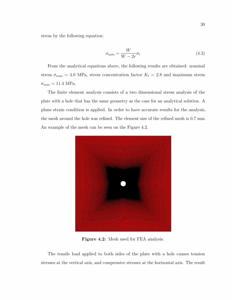
Figure 4.2: Mesh used for FEA analysis.

The tensile load applied to both sides of the plate with a hole causes tension

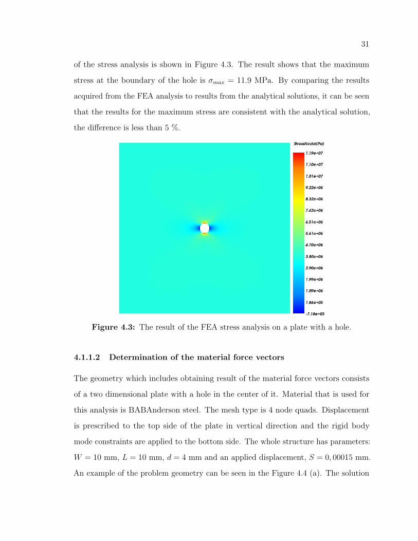
stresses at the vertical axis, and compressive stresses at the horizontal axis. The result

31

of the stress analysis is shown in Figure 4.3. The result shows that the maximum

stress at the boundary of the hole is σmax = 11.9 MPa. By comparing the results

acquired from the FEA analysis to results from the analytical solutions, it can be seen

that the results for the maximum stress are consistent with the analytical solution,

the difference is less than 5 %.

Figure 4.3: The result of the FEA stress analysis on a plate with a hole.

4.1.1.2 Determination of the material force vectors

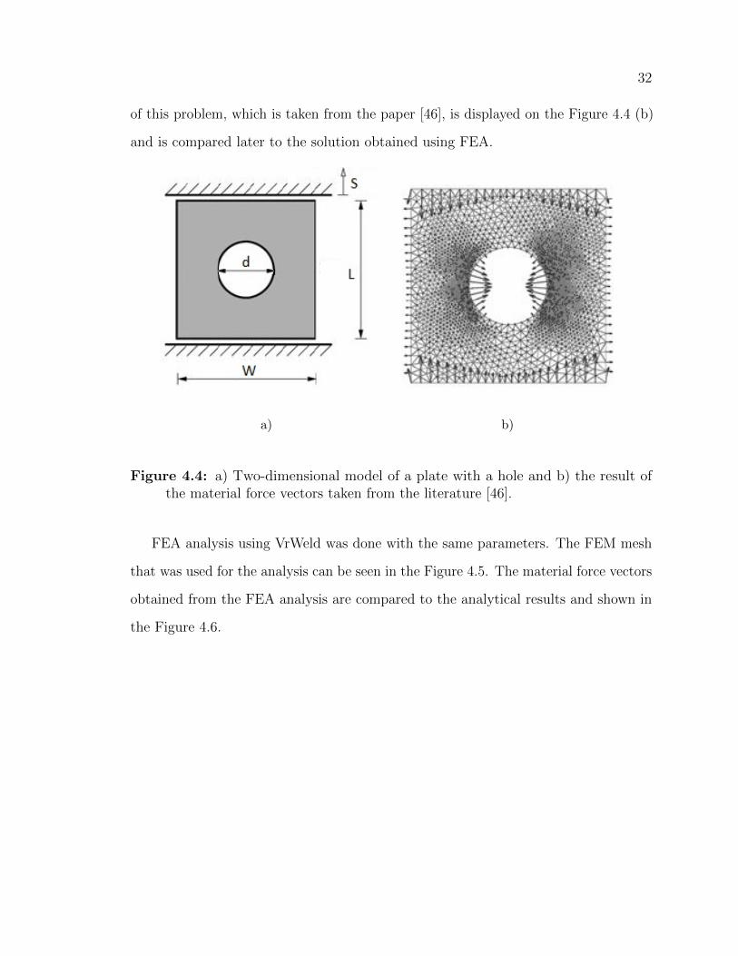
The geometry which includes obtaining result of the material force vectors consists

of a two dimensional plate with a hole in the center of it. Material that is used for

this analysis is BABAnderson steel. The mesh type is 4 node quads. Displacement

is prescribed to the top side of the plate in vertical direction and the rigid body

mode constraints are applied to the bottom side. The whole structure has parameters:

W = 10 mm, L = 10 mm, d = 4 mm and an applied displacement, S = 0, 00015 mm.

An example of the problem geometry can be seen in the Figure 4.4 (a). The solution

32

of this problem, which is taken from the paper [46], is displayed on the Figure 4.4 (b)

and is compared later to the solution obtained using FEA.

a) b)

Figure 4.4: a) Two-dimensional model of a plate with a hole and b) the result ofthe material force vectors taken from the literature [46].

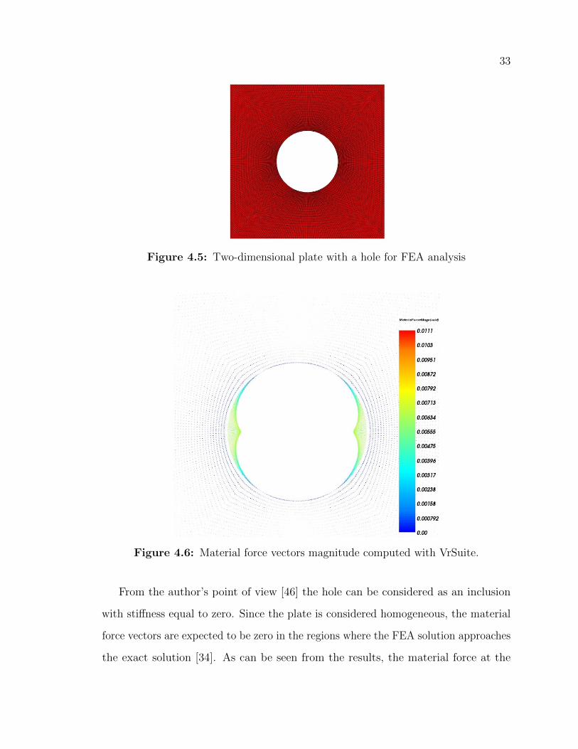
FEA analysis using VrWeld was done with the same parameters. The FEM mesh

that was used for the analysis can be seen in the Figure 4.5. The material force vectors

obtained from the FEA analysis are compared to the analytical results and shown in

the Figure 4.6.

33

Figure 4.5: Two-dimensional plate with a hole for FEA analysis

Figure 4.6: Material force vectors magnitude computed with VrSuite.

From the author’s point of view [46] the hole can be considered as an inclusion

with stiffness equal to zero. Since the plate is considered homogeneous, the material

force vectors are expected to be zero in the regions where the FEA solution approaches

the exact solution [34]. As can be seen from the results, the material force at the

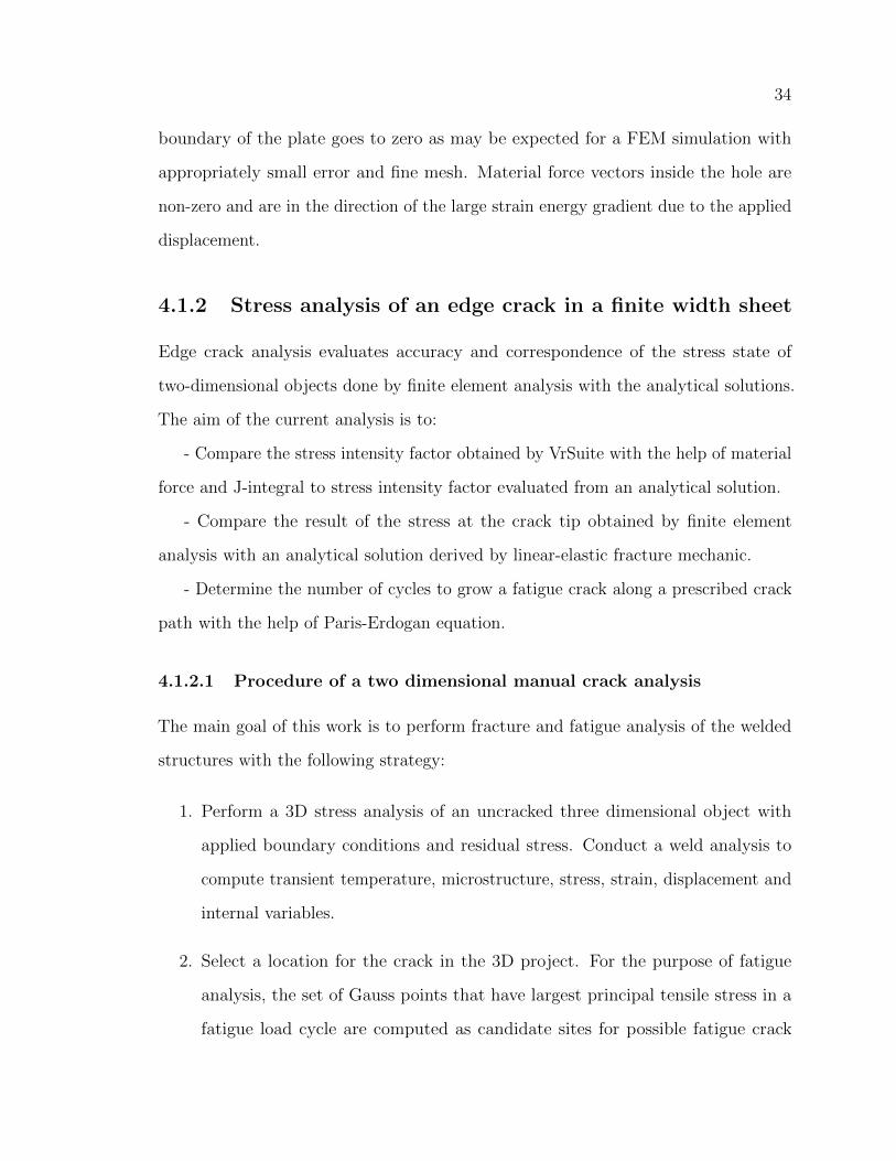
34

boundary of the plate goes to zero as may be expected for a FEM simulation with

appropriately small error and fine mesh. Material force vectors inside the hole are

non-zero and are in the direction of the large strain energy gradient due to the applied

displacement.

4.1.2 Stress analysis of an edge crack in a finite width sheet

Edge crack analysis evaluates accuracy and correspondence of the stress state of

two-dimensional objects done by finite element analysis with the analytical solutions.

The aim of the current analysis is to:

- Compare the stress intensity factor obtained by VrSuite with the help of material

force and J-integral to stress intensity factor evaluated from an analytical solution.

- Compare the result of the stress at the crack tip obtained by finite element

analysis with an analytical solution derived by linear-elastic fracture mechanic.

- Determine the number of cycles to grow a fatigue crack along a prescribed crack

path with the help of Paris-Erdogan equation.

4.1.2.1 Procedure of a two dimensional manual crack analysis

The main goal of this work is to perform fracture and fatigue analysis of the welded

structures with the following strategy:

1. Perform a 3D stress analysis of an uncracked three dimensional object with

applied boundary conditions and residual stress. Conduct a weld analysis to

compute transient temperature, microstructure, stress, strain, displacement and

internal variables.

2. Select a location for the crack in the 3D project. For the purpose of fatigue

analysis, the set of Gauss points that have largest principal tensile stress in a

fatigue load cycle are computed as candidate sites for possible fatigue crack

35

nucleation. In terms of fracture analysis, possible fracture locations are chosen

based on the Gauss points with highest principal stress and residual stresses.

3. In the current version, fracture and fatigue analysis are implemented for the

surface cracks, therefore the Gauss points that have the highest principal stress

values at the surface are selected. At the selected position, an elliptical crack

is placed with its center at the Gauss point and a crack plane normal to the

principal tensile stress. The width and depth of the elliptical crack are chosen

to be independent parameters.

4. Furthermore, a two dimensional fine plane strain mesh that is perpendicular to

the crack tip and normal to the crack surface is created. The position of the 2D

plane strain mesh can have different angles relatively to the crack. This plane

contains results of the stresses from the 3D analysis with no crack projected into

the face of the crack.

5. In each 2D mesh created, as described above, stresses are mapped from the

3D object with no crack to the mid-point of the corresponding face element on

the crack surface. Given the coordinates of the mid-point of face element on

the crack surface, the outward normal of the mid-point of face element on the

crack surface, the 3D stress tensor multiplies as a 3D matrix times the outward

normal to compute the tractions acting on the mid-point of each face element

on the crack surface. This traction is used to compute the Neumann boundary

conditions of the tractions acting on the crack faces of elements. In addition

Dirichlet boundary conditions are applied to constrain rigid body modes of the

two dimensional plane to zero. At the two bottom corners, the y-displacement is

constrained to zero and at the mid-point of the bottom edge, the x-displacement

is constrained to zero.

36

6. With this state and boundary conditions, the two dimensional plane strain

analysis of the fine crack mesh for one point on the crack tip is performed.

7. A plane strain analysis determines the material force at the crack tip that is

used for calculating of the J-integral and the stress intensity factor.

8. When the result of the material force vector is not clear, the value of the SIF is

computed from the CTOA on the crack faces near the crack tip.

9. Once the value of the stress intensity factor associated with each point on the

crack tip is known, it can be compared to the value of fracture toughness of the

structure in terms of fracture mechanics analysis.

10. For the purpose of fatigue analysis, (i.e. calculating the number of cycles to grow

for a crack), a crack with a new length has to be introduced. The location of

the crack, boundary conditions and parameters of the crack analysis remain the

same, as the crack length increases. This will allow to compute the increment of

the stress intensity factor of a new crack.

11. From the increment in the stress intensity factor, the rate of crack growth per

load cycle can be computed by solving the Paris-Erdogan equation.

12. An auto-report for fracture and fatigue analysis can be generated.

4.1.2.2 Determination of the stress intensity factor

The three dimensional plate, shown in Figure 4.7, with displacement applied to both

top and bottom of the plate in the vertical direction was created. The width of the

plate is 0.21 m, the length is 0.62 m and the thickness is 0.001 m. Material that is used

for this analysis is BABAnderson steel. The 3D FEM mesh consists of 8 node brick

elements and a mesh for a fine 2D crack analysis uses 4 node quads. A displacement of

37

0.00001 m is applied to the top and bottom sides and the z-displacement is constrained

to zero at all nodes in the plate to enforce the plane strain condition in the plate. The

result of the applied displacement in vertical direction can be seen in the Figure 4.7.

The dimensions of the 2D crack plate for analytical solution and FEA analysis

were chosen to be the same to be able to compare results. A general view of the

crack plane is shown in the Figure 4.9, where: b = 0.21 m, h = 0.31 m, a = 0.06 m,

S = 0.00001 m.

After performing a stress analysis of the two dimensional plate, the following result

of the displacement was obtained and is displayed in the Figure 4.8. As we can see

from Figure 4.8 b) during magnification of the displacement the crack is observed to

open, indicating that the results from the 3D object are mapped correctly.

Figure 4.7: Displacement field in the 3D plate without crack with prescribeddisplacement BCs at the top and bottom ends of 0.00001 m.

38

a) b)

Figure 4.8: a) Displacement in the 2D plate with a crack and b) displacement fieldmagnified 1000 times in the 2D plate with a crack.

The analytical solution of stress intensity factor KI for an edge crack caused by

mode I loading is obtained from the equation below [19].

KI = σ√πa[1.12− 0.23(

a

b) + 10.6(

a

b)2 − 21.7(

a

b)3 + 30.4(

a

b)4] (4.4)

This equation is valid for ratios of h/b ≥ 1.0 and a/b ≤ 0.6. The applied stress for

this equation can be simply derived from the displacement and is equal to 6.72 MPa.

The value of the analytical solution of stress intensity factor for this analysis is 4.71

MPa√m.

39

Figure 4.9: Two dimensional crack plane.

Stress intensity factor computed by VrSuite is evaluated with the help of the

J-integral by using the equation below:

KI =

√JE

1− ν2(4.5)

where J-integral is derived as the negative material force projected to the 2D crack

plane which is tangent to the crack path direction [35].

J = −Fmat · t (4.6)

The result of the material force solved by finite element analysis is displayed in the

Figure 4.10. The material force vector with the maximum value starts at the crack

tip and points in the direction opposite to the crack growth.

The computed stress intensity factor for an edge crack with the help of the equations

above has a value 4.59 MPa√m. The error between the analytical solution and the

computed solution is only 2.5 % which is considered a good agreement between

40

analytical and FEA results.

The obtained value of the stress intensity factor can be compared to the known

value of fracture toughness of the material, determined by the fracture toughness test,

to assess the resistance of the material to fracture.

a) b)

Figure 4.10: a) Material force vectors are shown near the crack tip and b) zoomedin section showing the material force vectors near the crack tip. The vectorshown in red is the material force vector acting on the crack tip.

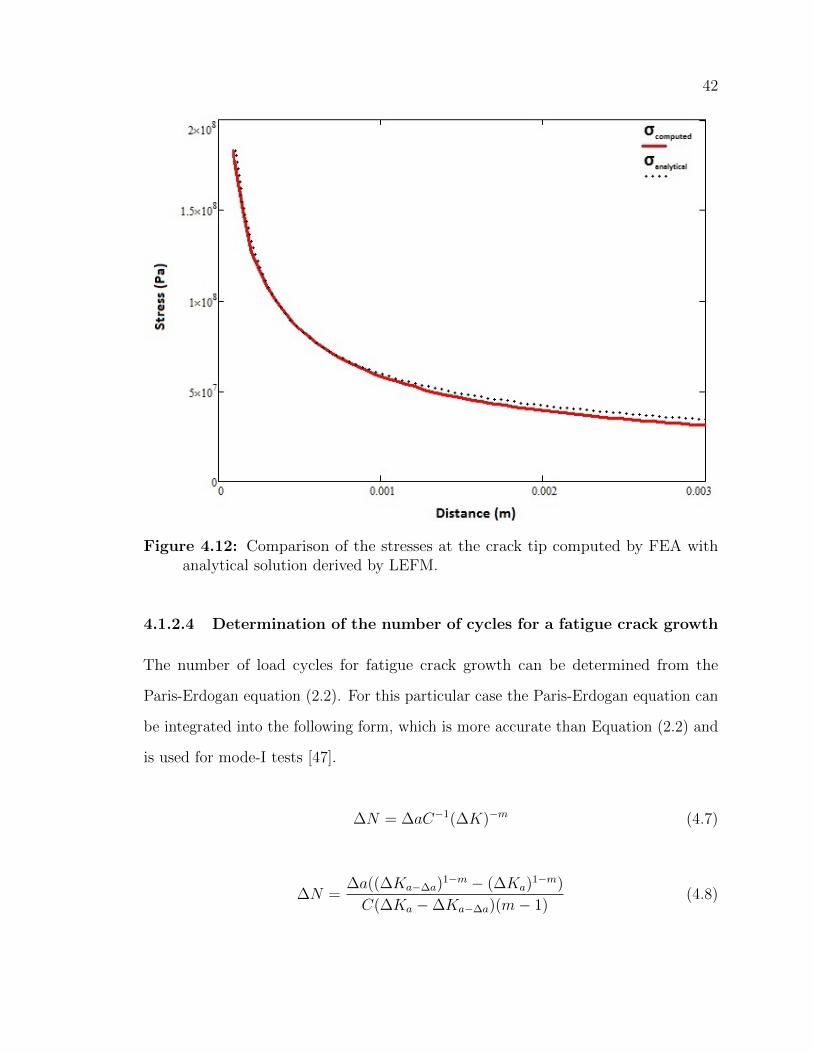
4.1.2.3 Comparison of the stress at the crack tip

From Section 2.4 we know that analytical stress derived under LEFM assumptions is

valid only for a certain ratio of the distance from the crack tip to crack length and

this ratio of r/a should be less than 0.05. Since the size of the crack is 0.06 m, the

distance from the crack tip should not exceed the value of 0.003 m.

The result of the computed nodal stress in xx direction with the help of FEA can

be found in Figure 4.11, with the highest value of 189 MPa. By knowing the value of

41

SIF for analytical solution of the stress under LEFM and using equation 2.1 we can

derive the values of the stress away from the crack tip. The highest value of the stress

for analytical solution is 187 MPa.

a) b)

Figure 4.11: a) The computed nodal stress in the xx direction for the 2D plate withthe crack and b) zoomed in result of the nodal stress in the xx direction for the2D plate with the crack.

To be able to compare results of the stress at the crack tip obtained by finite

element analysis with the analytical solution derived by linear-elastic fracture mechanic

the plot of the stress versus distance from the crack tip was made and displayed in

Figure 4.12. It may be observed from the plot that the FEM results are consistent

with the analytical solution.

42

Figure 4.12: Comparison of the stresses at the crack tip computed by FEA withanalytical solution derived by LEFM.

4.1.2.4 Determination of the number of cycles for a fatigue crack growth

The number of load cycles for fatigue crack growth can be determined from the

Paris-Erdogan equation (2.2). For this particular case the Paris-Erdogan equation can

be integrated into the following form, which is more accurate than Equation (2.2) and

is used for mode-I tests [47].

∆N = ∆aC−1(∆K)−m (4.7)

∆N =∆a((∆Ka−∆a)

1−m − (∆Ka)1−m)

C(∆Ka −∆Ka−∆a)(m− 1)(4.8)

43

Where ∆a is an increment in crack length in the load cycles; ∆Ka equals to the value

of ∆K when the crack length is a; ∆Ka−∆a is equal to the value of ∆K when the

crack length is a−∆a.

The following analysis was done with the same value of applied displacement,

geometry and parameters as for calculation of the stress intensity factor. Initial crack

length equal to 0.06 m. The crack increment for this case is 0.01 m. The crack was

grown from the value of 0.06 m to 0.07 m. The value of the stress intensity factor

for the final crack is 5.84 MPa. The values of the Paris-Erdogan constants for the

analysis are chosen to be C = 6.9× 10−12(m/cycles)(MPa√m)−m and m = 3.0.

Equation 4.8 was used to determine that the number of cycles to grow the fatigue

crack from 0.06 m to 0.07 m for the given material is equal to 10,508,142 cycles.

4.2 Manual fatigue analysis of the laser weld

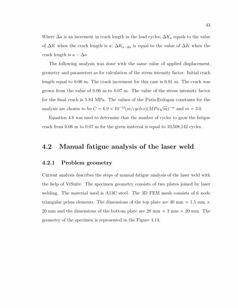
4.2.1 Problem geometry

Current analysis describes the steps of manual fatigue analysis of the laser weld with

the help of VrSuite. The specimen geometry consists of two plates joined by laser

welding. The material used is A13C steel. The 3D FEM mesh consists of 6 node

triangular prism elements. The dimensions of the top plate are 40 mm × 1.5 mm ×

20 mm and the dimensions of the bottom plate are 28 mm × 3 mm × 20 mm. The

geometry of the specimen is represented in the Figure 4.13.

44

Figure 4.13: Geometry of the specimen. Triad axes: red is the X axis, yellow is theY axis, green is the Z axis.

4.2.2 Setup and analysis

Once the mesh is created and the welding is simulated the following steps are done in

order to manually analyse the laser weld specimen:

• A tensile load of 100 MPa is applied to the top right and bottom left parts of the

sample and rigid body modes are constrained. A weld analysis that computes

transient temperature, microstructure and stress is performed.

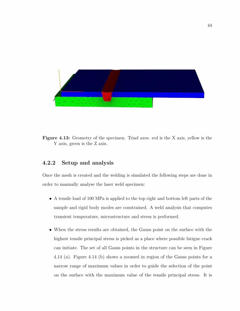
• When the stress results are obtained, the Gauss point on the surface with the

highest tensile principal stress is picked as a place where possible fatigue crack

can initiate. The set of all Gauss points in the structure can be seen in Figure

4.14 (a). Figure 4.14 (b) shows a zoomed in region of the Gauss points for a

narrow range of maximum values in order to guide the selection of the point

on the surface with the maximum value of the tensile principal stress. It is

45

assumed that the structure doesn’t have a crack due to the welding and crack

nucleates because of the residual stresses after welding and in-service loading of

the specimen.

a) b)

Figure 4.14: a) Result of the Gauss points that show a principal stress in thestructure b) Zoomed in region of the Gauss points with narrow range of themaximum values.

• Once the node is picked, an elliptical crack is created with the center at the

chosen Gauss point. The length of the ellipse for current analysis is set to 1.6

mm and the width is 1 mm. The 2D crack plane is created normal to an elliptical

crack and in plane with the applied tensile load. The crack length is set to 0.5

mm. The mesh of an elliptical crack with perpendicular to it 2D crack plane is

shown in Figure 4.15.

46

Figure 4.15: Example of an elliptical crack mesh that is perpendicular to the 2Dplane strain mesh

• After setting the crack analysis parameters and running the project with a crack,

the following result of the material force was acquired and depicted in Figure

4.16. The highest value of the material force was found to be 1.91× 103. Using

equations 4.5 and 4.6 the values of the J-integral and SIF are derived. The stress

intensity factor for a crack length of 1 mm is 20.9 MPa√m.

47

Figure 4.16: Material force vectors competed with VrSuite for a crack length of 0.5mm.

• In order to compute the number of cycles needed for crack to grow from 0.5

mm to 0.7 mm, a crack is extended to a length of 0.7 mm. The same analysis

parameters and boundary conditions are used as in the analysis above. The

result of the material force is shown on the Figure 4.17 with the highest value of

6.94× 103. The SIF for this crack length is 40 MPa√m.

48

Figure 4.17: Material force vectors competed with VrSuite for a crack length of 0.7mm.

• Knowing values of the SIF for both cases give a possibility to determine the

number of load cycles needed for fatigue crack growth from 0.5 mm to 0.7 mm.

Material constants for the analysis are C = 6.9× 10−12(m/cycles)(MPa√m)−m

and m = 3.0. The Paris-Erdogan equation 4.8 was used to determine that 1,262

cycles are necessary to grow the crack to the prescribed length.

4.3 Automation of the fatigue analysis process

Automation of the fatigue analysis process of welded structures can play an important

role for industries in terms of saving time and avoiding manual mistakes done by a

49

user while setting an analysis. Automation of the algorithm above for fracture and

fatigue analysis can also help a user to analyse more structures at the same time.

The following steps have been done in order to simplify and automate the process

of fracture analysis for a user:

1. Instead of the user’s manual picking of a Gauss point with a highest value of

the principal stress for possible location of fatigue crack, a set of Gauss points is

chosen automatically, based on the value of highest principal stress. A set of

points can have 1, 2 or 10 possible locations of cracks.

2. A fine crack mesh with a center at the Gauss point is created automatically at

each chosen point. The user can then set desired value for the radius of the

crack.

3. A plain strain crack mesh that is perpendicular to the crack mesh is created

automatically for each Gauss point. The user is prompted to set an angle for a

plane strain mesh with respect to a crack mesh.

4. For each specified point on the crack tip curve, a plane strain analysis is done

with result values of the stress, displacement and material force.

5. From the result of material force at each point on the crack tip, the stress

intensity factor is calculated automatically.

6. If the result of the material force vector is not clear, the value of the SIF is

computed automatically from the CTOA.

7. In terms of fracture analysis, the stress intensity factor is compared to the

fracture toughness of the material to predict the risk of fracture.

8. The obtained results of stress intensity factor increment would allow the Paris-

Erdogan equation to be solved automatically to determine the number of cycles

50

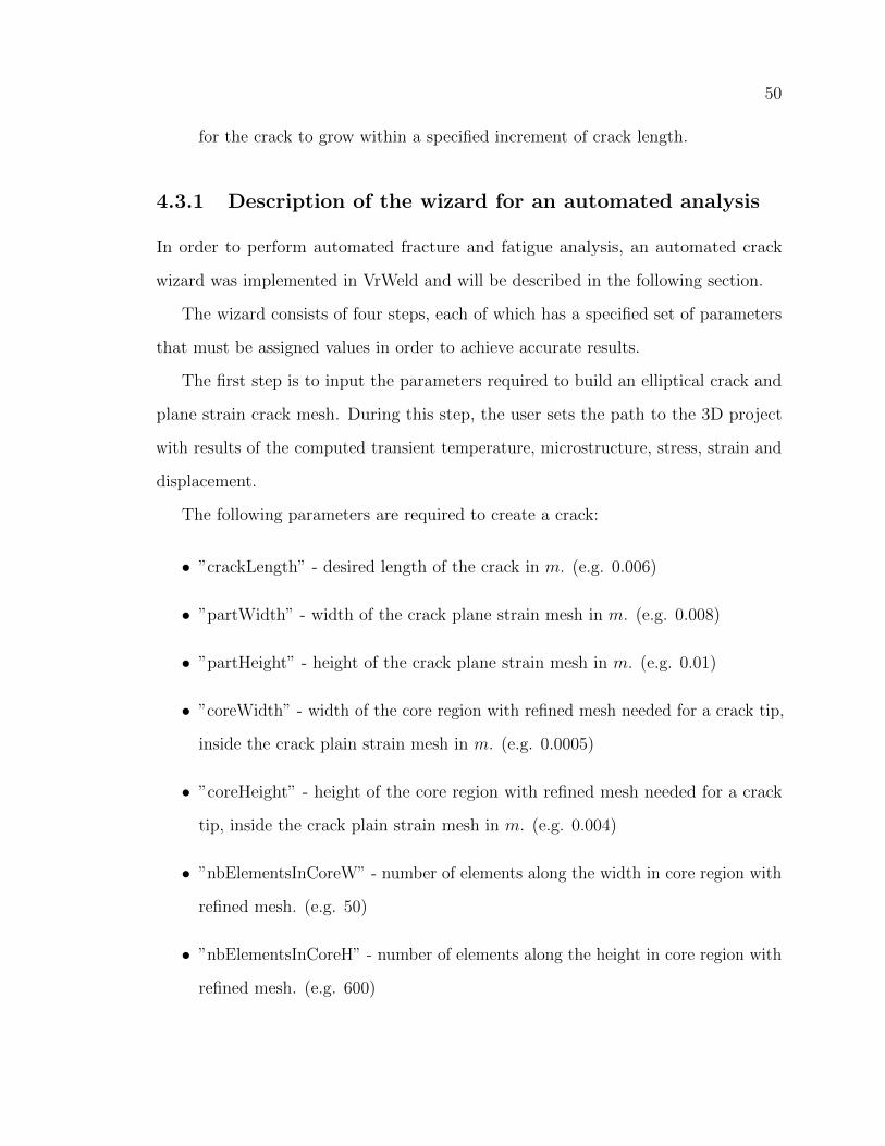
for the crack to grow within a specified increment of crack length.

4.3.1 Description of the wizard for an automated analysis

In order to perform automated fracture and fatigue analysis, an automated crack

wizard was implemented in VrWeld and will be described in the following section.

The wizard consists of four steps, each of which has a specified set of parameters

that must be assigned values in order to achieve accurate results.

The first step is to input the parameters required to build an elliptical crack and

plane strain crack mesh. During this step, the user sets the path to the 3D project

with results of the computed transient temperature, microstructure, stress, strain and

displacement.

The following parameters are required to create a crack:

• ”crackLength” - desired length of the crack in m. (e.g. 0.006)

• ”partWidth” - width of the crack plane strain mesh in m. (e.g. 0.008)

• ”partHeight” - height of the crack plane strain mesh in m. (e.g. 0.01)

• ”coreWidth” - width of the core region with refined mesh needed for a crack tip,

inside the crack plain strain mesh in m. (e.g. 0.0005)

• ”coreHeight” - height of the core region with refined mesh needed for a crack

tip, inside the crack plain strain mesh in m. (e.g. 0.004)

• ”nbElementsInCoreW” - number of elements along the width in core region with

refined mesh. (e.g. 50)

• ”nbElementsInCoreH” - number of elements along the height in core region with

refined mesh. (e.g. 600)

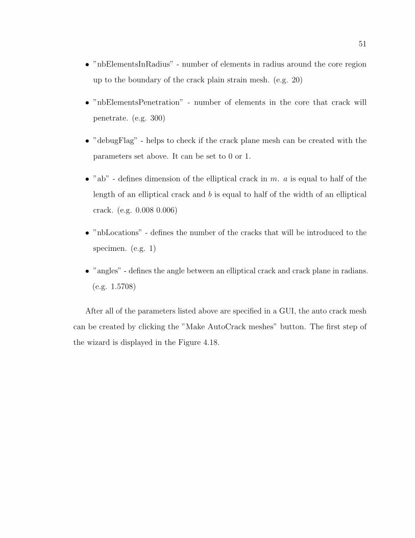
51

• ”nbElementsInRadius” - number of elements in radius around the core region

up to the boundary of the crack plain strain mesh. (e.g. 20)

• ”nbElementsPenetration” - number of elements in the core that crack will

penetrate. (e.g. 300)

• ”debugFlag” - helps to check if the crack plane mesh can be created with the

parameters set above. It can be set to 0 or 1.

• ”ab” - defines dimension of the elliptical crack in m. a is equal to half of the

length of an elliptical crack and b is equal to half of the width of an elliptical

crack. (e.g. 0.008 0.006)

• ”nbLocations” - defines the number of the cracks that will be introduced to the

specimen. (e.g. 1)

• ”angles” - defines the angle between an elliptical crack and crack plane in radians.

(e.g. 1.5708)

After all of the parameters listed above are specified in a GUI, the auto crack mesh

can be created by clicking the ”Make AutoCrack meshes” button. The first step of

the wizard is displayed in the Figure 4.18.

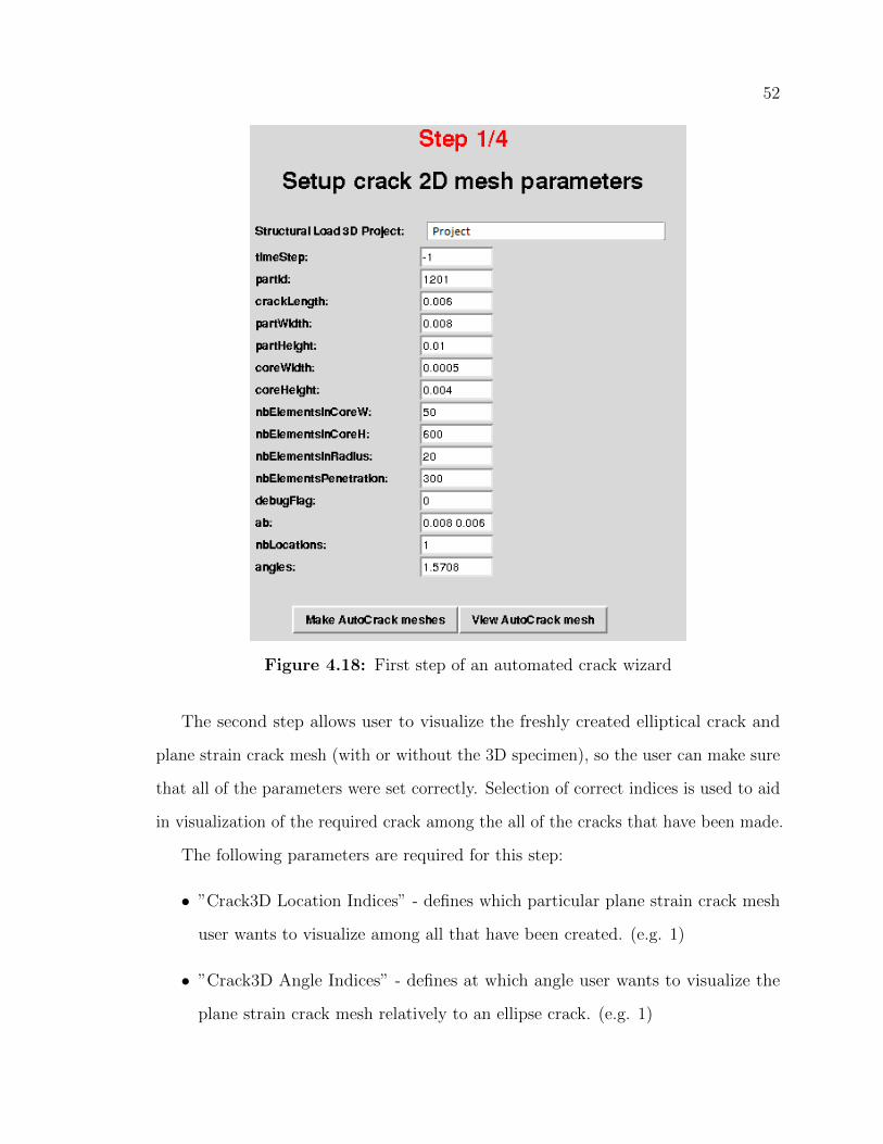
52

Figure 4.18: First step of an automated crack wizard

The second step allows user to visualize the freshly created elliptical crack and

plane strain crack mesh (with or without the 3D specimen), so the user can make sure

that all of the parameters were set correctly. Selection of correct indices is used to aid

in visualization of the required crack among the all of the cracks that have been made.

The following parameters are required for this step:

• ”Crack3D Location Indices” - defines which particular plane strain crack mesh

user wants to visualize among all that have been created. (e.g. 1)

• ”Crack3D Angle Indices” - defines at which angle user wants to visualize the

plane strain crack mesh relatively to an ellipse crack. (e.g. 1)

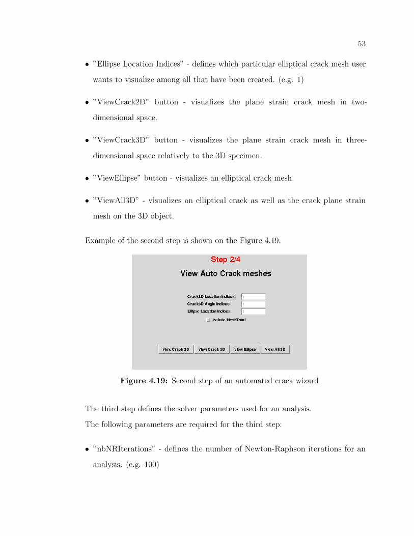
53

• ”Ellipse Location Indices” - defines which particular elliptical crack mesh user

wants to visualize among all that have been created. (e.g. 1)

• ”ViewCrack2D” button - visualizes the plane strain crack mesh in two-

dimensional space.

• ”ViewCrack3D” button - visualizes the plane strain crack mesh in three-

dimensional space relatively to the 3D specimen.

• ”ViewEllipse” button - visualizes an elliptical crack mesh.

• ”ViewAll3D” - visualizes an elliptical crack as well as the crack plane strain

mesh on the 3D object.

Example of the second step is shown on the Figure 4.19.

Figure 4.19: Second step of an automated crack wizard

The third step defines the solver parameters used for an analysis.

The following parameters are required for the third step:

• ”nbNRIterations” - defines the number of Newton-Raphson iterations for an

analysis. (e.g. 100)

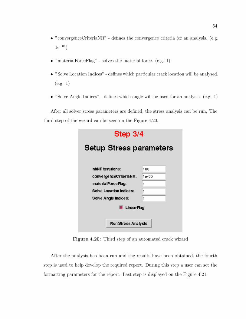
54

• ”convergenceCriteriaNR” - defines the convergence criteria for an analysis. (e.g.

1e−05)

• ”materialForceFlag” - solves the material force. (e.g. 1)

• ”Solve Location Indices” - defines which particular crack location will be analysed.

(e.g. 1)

• ”Solve Angle Indices” - defines which angle will be used for an analysis. (e.g. 1)

After all solver stress parameters are defined, the stress analysis can be run. The

third step of the wizard can be seen on the Figure 4.20.

Figure 4.20: Third step of an automated crack wizard

After the analysis has been run and the results have been obtained, the fourth

step is used to help develop the required report. During this step a user can set the

formatting parameters for the report. Last step is displayed on the Figure 4.21.

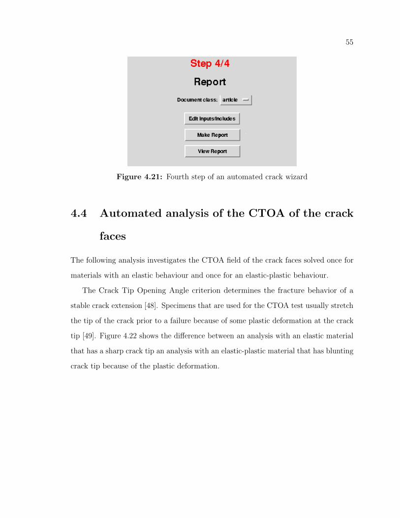
55

Figure 4.21: Fourth step of an automated crack wizard

4.4 Automated analysis of the CTOA of the crack

faces

The following analysis investigates the CTOA field of the crack faces solved once for

materials with an elastic behaviour and once for an elastic-plastic behaviour.

The Crack Tip Opening Angle criterion determines the fracture behavior of a

stable crack extension [48]. Specimens that are used for the CTOA test usually stretch

the tip of the crack prior to a failure because of some plastic deformation at the crack

tip [49]. Figure 4.22 shows the difference between an analysis with an elastic material

that has a sharp crack tip an analysis with an elastic-plastic material that has blunting

crack tip because of the plastic deformation.

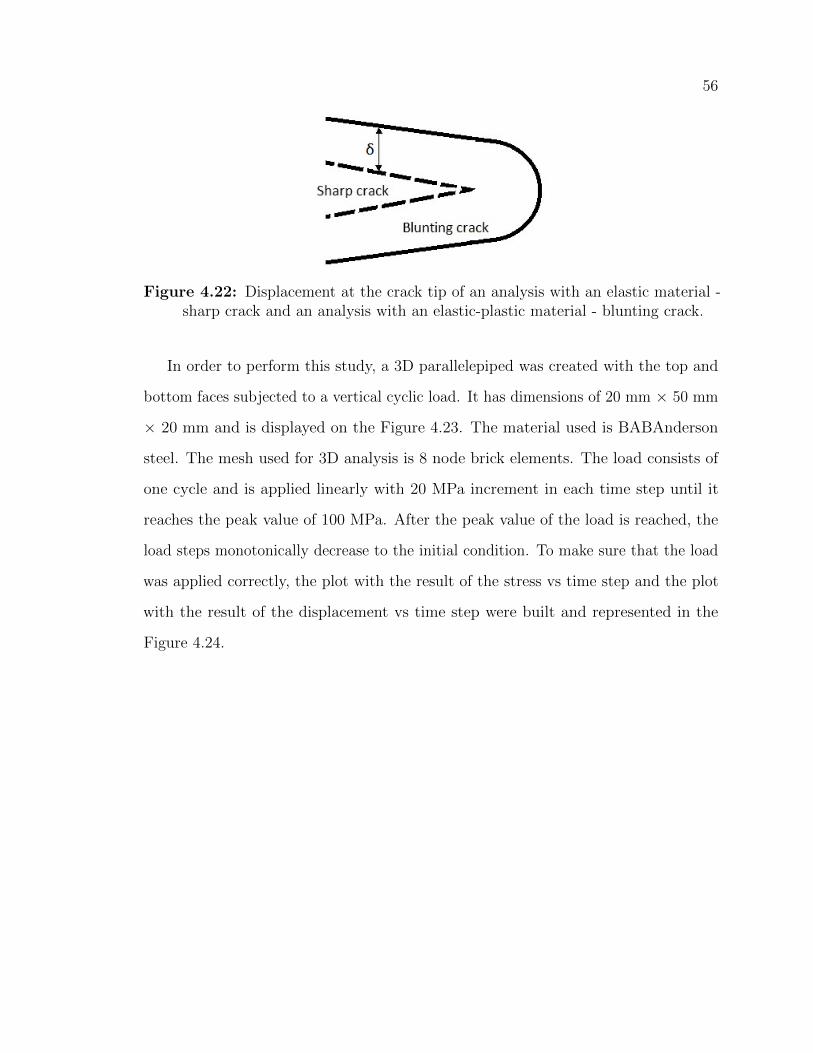
56

Figure 4.22: Displacement at the crack tip of an analysis with an elastic material -sharp crack and an analysis with an elastic-plastic material - blunting crack.

In order to perform this study, a 3D parallelepiped was created with the top and

bottom faces subjected to a vertical cyclic load. It has dimensions of 20 mm × 50 mm

× 20 mm and is displayed on the Figure 4.23. The material used is BABAnderson

steel. The mesh used for 3D analysis is 8 node brick elements. The load consists of

one cycle and is applied linearly with 20 MPa increment in each time step until it

reaches the peak value of 100 MPa. After the peak value of the load is reached, the

load steps monotonically decrease to the initial condition. To make sure that the load

was applied correctly, the plot with the result of the stress vs time step and the plot

with the result of the displacement vs time step were built and represented in the

Figure 4.24.

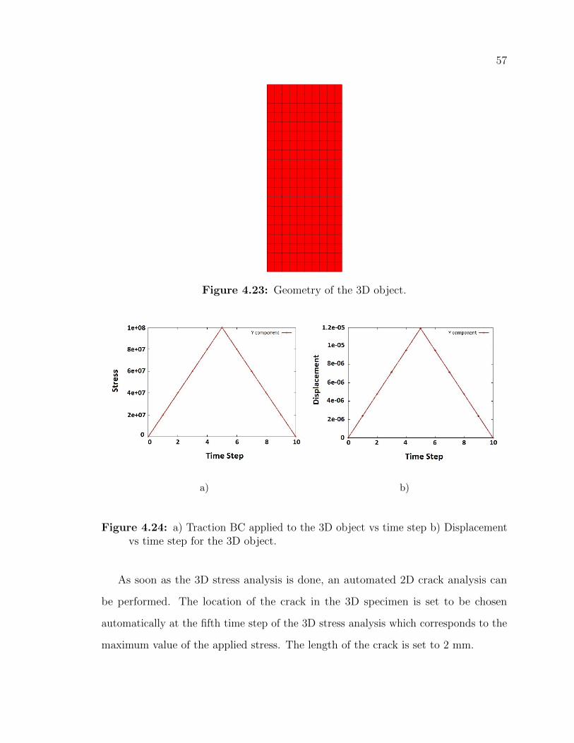
57

Figure 4.23: Geometry of the 3D object.

a) b)

Figure 4.24: a) Traction BC applied to the 3D object vs time step b) Displacementvs time step for the 3D object.

As soon as the 3D stress analysis is done, an automated 2D crack analysis can

be performed. The location of the crack in the 3D specimen is set to be chosen

automatically at the fifth time step of the 3D stress analysis which corresponds to the

maximum value of the applied stress. The length of the crack is set to 2 mm.

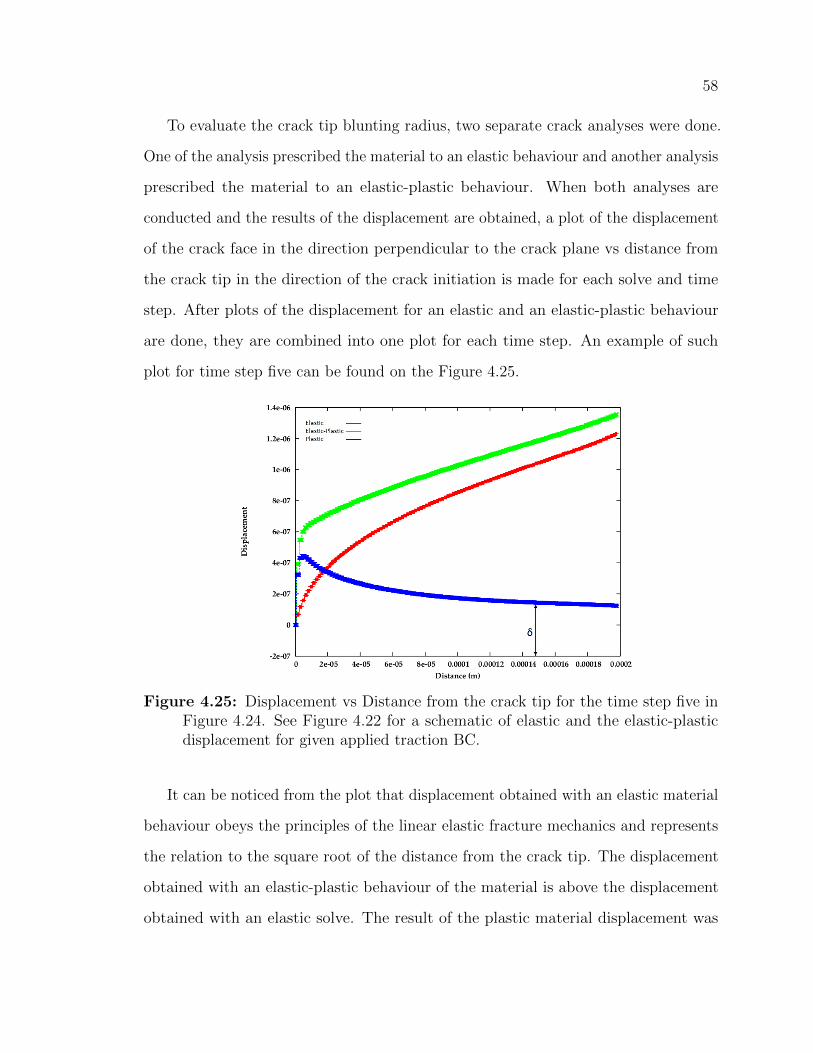
58

To evaluate the crack tip blunting radius, two separate crack analyses were done.

One of the analysis prescribed the material to an elastic behaviour and another analysis

prescribed the material to an elastic-plastic behaviour. When both analyses are

conducted and the results of the displacement are obtained, a plot of the displacement

of the crack face in the direction perpendicular to the crack plane vs distance from

the crack tip in the direction of the crack initiation is made for each solve and time

step. After plots of the displacement for an elastic and an elastic-plastic behaviour

are done, they are combined into one plot for each time step. An example of such

plot for time step five can be found on the Figure 4.25.

Figure 4.25: Displacement vs Distance from the crack tip for the time step five inFigure 4.24. See Figure 4.22 for a schematic of elastic and the elastic-plasticdisplacement for given applied traction BC.

It can be noticed from the plot that displacement obtained with an elastic material

behaviour obeys the principles of the linear elastic fracture mechanics and represents

the relation to the square root of the distance from the crack tip. The displacement

obtained with an elastic-plastic behaviour of the material is above the displacement

obtained with an elastic solve. The result of the plastic material displacement was

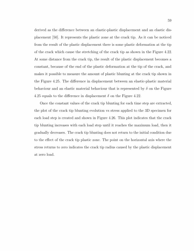
59

derived as the difference between an elastic-plastic displacement and an elastic dis-

placement [50]. It represents the plastic zone at the crack tip. As it can be noticed

from the result of the plastic displacement there is some plastic deformation at the tip

of the crack which cause the stretching of the crack tip as shown in the Figure 4.22.

At some distance from the crack tip, the result of the plastic displacement becomes a

constant, because of the end of the plastic deformation at the tip of the crack, and

makes it possible to measure the amount of plastic blunting at the crack tip shown in

the Figure 4.25. The difference in displacement between an elastic-plastic material

behaviour and an elastic material behaviour that is represented by δ on the Figure

4.25 equals to the difference in displacement δ on the Figure 4.22.

Once the constant values of the crack tip blunting for each time step are extracted,

the plot of the crack tip blunting evolution vs stress applied to the 3D specimen for

each load step is created and shown in Figure 4.26. This plot indicates that the crack

tip blunting increases with each load step until it reaches the maximum load, then it

gradually decreases. The crack tip blunting does not return to the initial condition due

to the effect of the crack tip plastic zone. The point on the horizontal axis where the

stress returns to zero indicates the crack tip radius caused by the plastic displacement

at zero load.

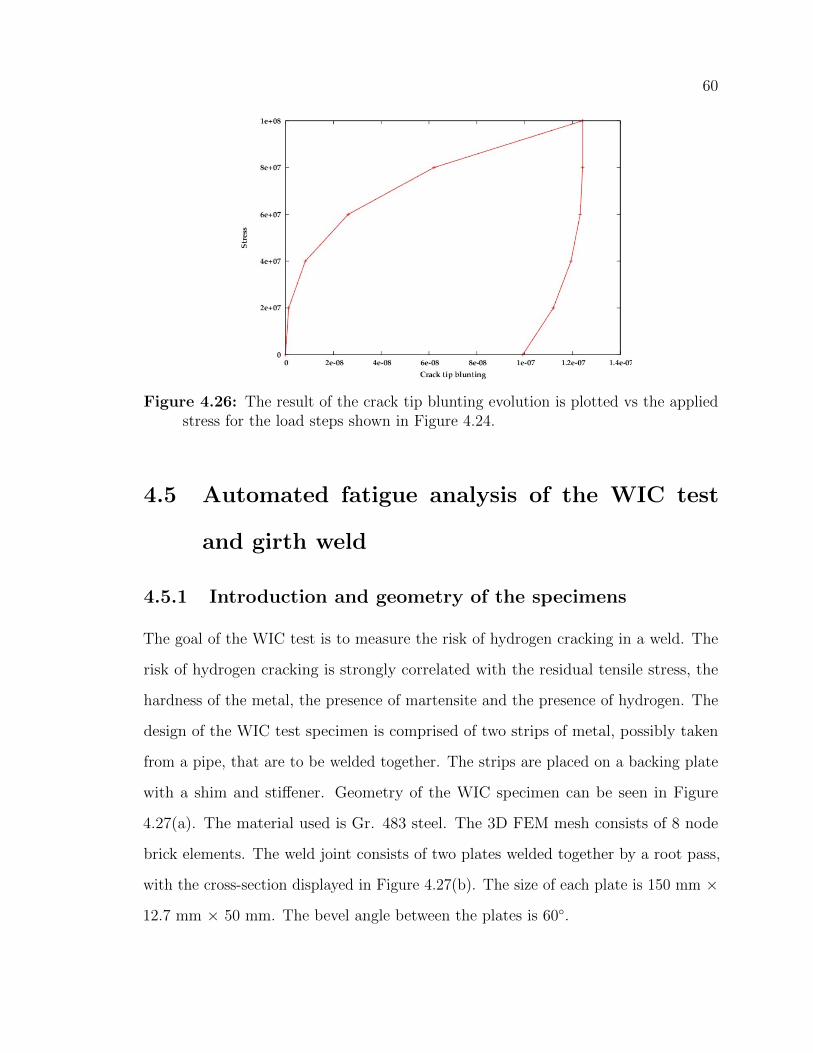
60

Figure 4.26: The result of the crack tip blunting evolution is plotted vs the appliedstress for the load steps shown in Figure 4.24.

4.5 Automated fatigue analysis of the WIC test

and girth weld

4.5.1 Introduction and geometry of the specimens

The goal of the WIC test is to measure the risk of hydrogen cracking in a weld. The

risk of hydrogen cracking is strongly correlated with the residual tensile stress, the

hardness of the metal, the presence of martensite and the presence of hydrogen. The

design of the WIC test specimen is comprised of two strips of metal, possibly taken

from a pipe, that are to be welded together. The strips are placed on a backing plate

with a shim and stiffener. Geometry of the WIC specimen can be seen in Figure

4.27(a). The material used is Gr. 483 steel. The 3D FEM mesh consists of 8 node

brick elements. The weld joint consists of two plates welded together by a root pass,

with the cross-section displayed in Figure 4.27(b). The size of each plate is 150 mm ×

12.7 mm × 50 mm. The bevel angle between the plates is 60◦.

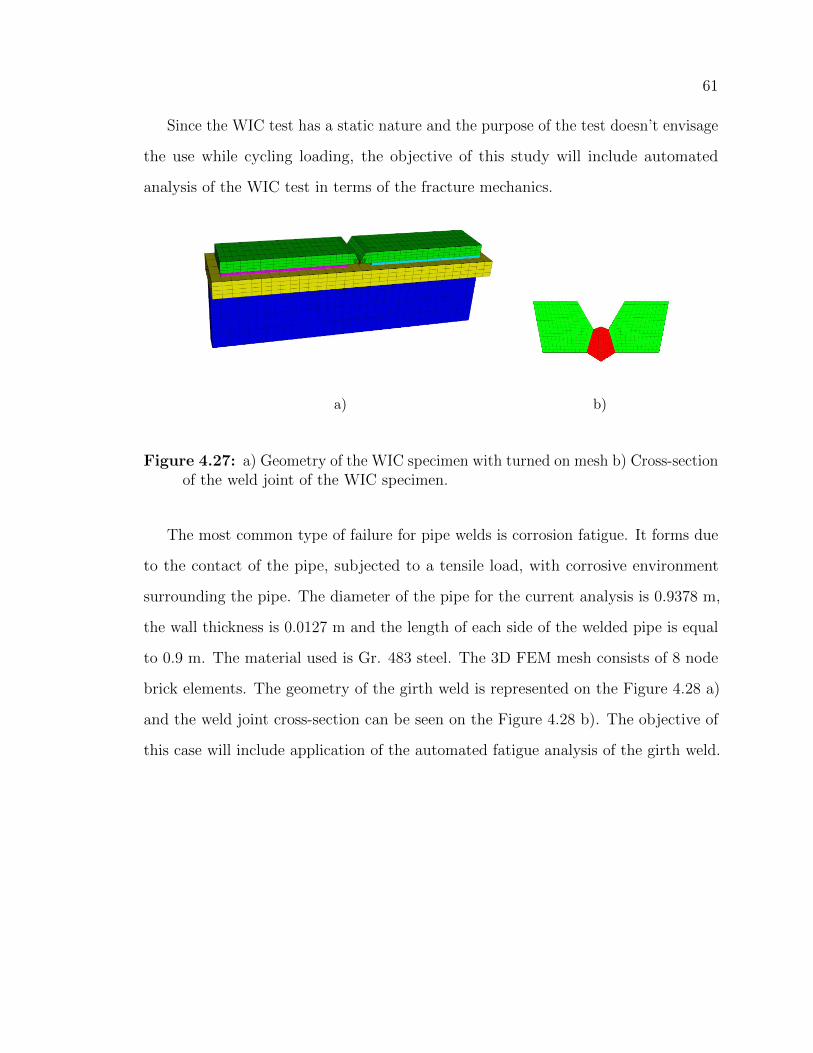
61

Since the WIC test has a static nature and the purpose of the test doesn’t envisage

the use while cycling loading, the objective of this study will include automated

analysis of the WIC test in terms of the fracture mechanics.

a) b)

Figure 4.27: a) Geometry of the WIC specimen with turned on mesh b) Cross-sectionof the weld joint of the WIC specimen.

The most common type of failure for pipe welds is corrosion fatigue. It forms due

to the contact of the pipe, subjected to a tensile load, with corrosive environment

surrounding the pipe. The diameter of the pipe for the current analysis is 0.9378 m,

the wall thickness is 0.0127 m and the length of each side of the welded pipe is equal

to 0.9 m. The material used is Gr. 483 steel. The 3D FEM mesh consists of 8 node

brick elements. The geometry of the girth weld is represented on the Figure 4.28 a)

and the weld joint cross-section can be seen on the Figure 4.28 b). The objective of

this case will include application of the automated fatigue analysis of the girth weld.

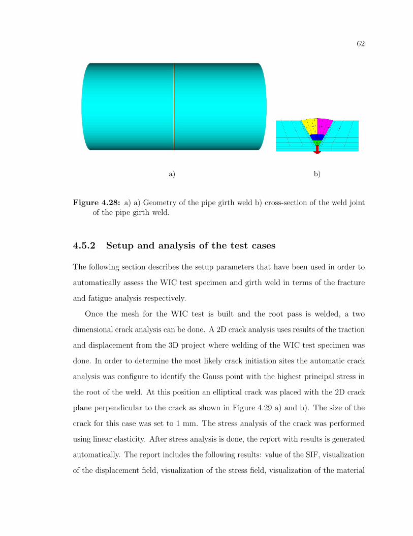
62

a) b)

Figure 4.28: a) a) Geometry of the pipe girth weld b) cross-section of the weld jointof the pipe girth weld.

4.5.2 Setup and analysis of the test cases

The following section describes the setup parameters that have been used in order to

automatically assess the WIC test specimen and girth weld in terms of the fracture

and fatigue analysis respectively.

Once the mesh for the WIC test is built and the root pass is welded, a two

dimensional crack analysis can be done. A 2D crack analysis uses results of the traction

and displacement from the 3D project where welding of the WIC test specimen was

done. In order to determine the most likely crack initiation sites the automatic crack

analysis was configure to identify the Gauss point with the highest principal stress in

the root of the weld. At this position an elliptical crack was placed with the 2D crack

plane perpendicular to the crack as shown in Figure 4.29 a) and b). The size of the

crack for this case was set to 1 mm. The stress analysis of the crack was performed

using linear elasticity. After stress analysis is done, the report with results is generated

automatically. The report includes the following results: value of the SIF, visualization

of the displacement field, visualization of the stress field, visualization of the material

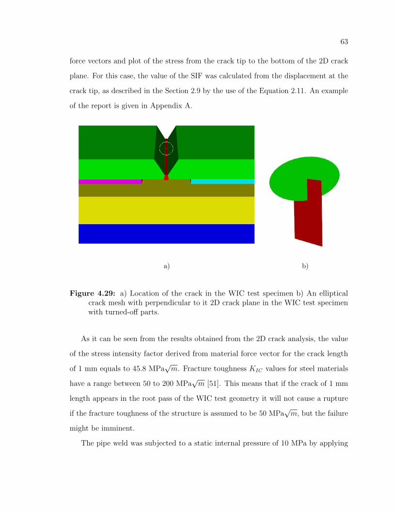
63

force vectors and plot of the stress from the crack tip to the bottom of the 2D crack

plane. For this case, the value of the SIF was calculated from the displacement at the

crack tip, as described in the Section 2.9 by the use of the Equation 2.11. An example

of the report is given in Appendix A.

a) b)

Figure 4.29: a) Location of the crack in the WIC test specimen b) An ellipticalcrack mesh with perpendicular to it 2D crack plane in the WIC test specimenwith turned-off parts.

As it can be seen from the results obtained from the 2D crack analysis, the value

of the stress intensity factor derived from material force vector for the crack length

of 1 mm equals to 45.8 MPa√m. Fracture toughness KIC values for steel materials

have a range between 50 to 200 MPa√m [51]. This means that if the crack of 1 mm

length appears in the root pass of the WIC test geometry it will not cause a rupture

if the fracture toughness of the structure is assumed to be 50 MPa√m, but the failure

might be imminent.

The pipe weld was subjected to a static internal pressure of 10 MPa by applying

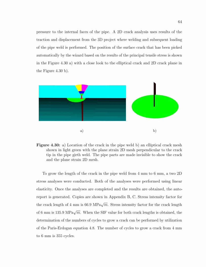
64

pressure to the internal faces of the pipe. A 2D crack analysis uses results of the

traction and displacement from the 3D project where welding and subsequent loading

of the pipe weld is performed. The position of the surface crack that has been picked

automatically by the wizard based on the results of the principal tensile stress is shown

in the Figure 4.30 a) with a close look to the elliptical crack and 2D crack plane in

the Figure 4.30 b).

a) b)

Figure 4.30: a) Location of the crack in the pipe weld b) an elliptical crack meshshown in light green with the plane strain 2D mesh perpendicular to the cracktip in the pipe girth weld. The pipe parts are made invisible to show the crackand the plane strain 2D mesh.

To grow the length of the crack in the pipe weld from 4 mm to 6 mm, a two 2D

stress analyses were conducted. Both of the analyses were performed using linear

elasticity. Once the analyses are completed and the results are obtained, the auto-

report is generated. Copies are shown in Appendix B, C. Stress intensity factor for

the crack length of 4 mm is 66.9 MPa√m. Stress intensity factor for the crack length

of 6 mm is 135.9 MPa√m. When the SIF value for both crack lengths is obtained, the

determination of the numbers of cycles to grow a crack can be performed by utilization

of the Paris-Erdogan equation 4.8. The number of cycles to grow a crack from 4 mm

to 6 mm is 355 cycles.

Chapter 5

Conclusion and possible future works

The current work reviews several studies conducted on fatigue analysis in Section 1.2.

By analysing works performed by other researches it was feasible to identify possible

extension of scope in fatigue analysis, as well as to define new areas of study.

The assessment of residual life of the welded structures in this thesis is done through

development of an algorithm for performing fracture mechanics analysis and fatigue

analysis using the VrSuite software. The objectives of this investigation included:

• Define an algorithm to automate the determination of the linear elastic stress

intensity factors in welding components containing residual stresses due to

welding in combination due to in-service loads;

• Predict the crack rate of crack propagation in the welded structures due to

in-service load cycles;

Initially, VrSuite software was verified by comparison to computed stress results

with an analytical solution. For this purpose, in Sections 4.1.1.1, an analysis was

conducted on a 2D plate with a hole in the center of it subjected to tensile load. The

idea of this test was to compute the maximum stress in the plate and compare it to

an established analytical solution. As a result, the comparison of results showed a

good agreement with an error of less than 5%. Later in this section the direction of

65

66

the material force vectors was compared to the one obtained from the literature. As

can be seen from the comparison in Section 4.1.1.2, the distribution of material force

vectors computed by VrSuite is consistent with result of material force vector taken

from the paper [46].

After verification of the stress results obtained by VrSuite an edge crack was

introduced into the 3D plate with displacement applied to the top and bottom side of

the plate as described in Section 4.1.2.2. The aim of the analysis was to compare the

result of the stress intensity factor computed by FEM with the help of the material

force and J-integral to the value derived by using the analytical equation taken

from [20] for an edge crack, to verify the results obtained by VrSuite. As can be

seen in Section 4.1.2.2, the stress intensity result obtained by FEA had an error of

only 2.5 % compared to an analytical solution which indicates a good agreement

between the results. In section 4.1.2.4 a modified form of the Paris-Erdogan equation

is implemented to compute the number of load cycles required to grow a crack to a

specified size.

Section 4.2 describes the procedure for conducting a manual fatigue analysis for a

laser weld. It includes a description of the geometry used for analysis and provides

information on the setup and parameters used in this case as well as discussion of the

obtained results.

A description of the automated fatigue analysis is given in Section 4.3. The section

concentrates on the difference between manual and automated fatigue and fracture

analysis of the welded components. An explanation of the role of the wizard and steps

of the automated analysis is given.

The use of an automated fracture and fatigue analysis is presented for a WIC test

specimen and a pipe girth weld. Section 4.5 includes information about the geometry

of each specimen and parameters that were used for each case as well as provides the

results obtained from the automated analysis.

67

5.1 Future direction of work

Although the research described in this thesis has provided new insight into an

automated fatigue and fracture analysis of welded components, there are opportunities

for improvement. This section expands upon some potential enhancements that may

be incorporated in future work:

• Extend the ability to analyze not only surface cracks but sub-surface cracks as

well.

• Perform further analysis on additional specimens with varying geometries, in-

cluding the cases with gusset joints.

• Perform analysis with cycling load patterns.

• Implement an algorithm for predicting fatigue crack growth based on Pommier’s

time-derivative crack propagation equations [50].

References

[1] Stout R.D., Wayman C.M. A study of factors affecting the strength and ductility

of weld metal. Welding Journal, 5, May 1958.

[2] Harrison J.D. Lessons from service fatigue failures. The Welding Institute Research

Bulletin, 12, March 1980.

[3] Rethwisch D. G., Callister W. D. Materials science and engineering: An intro-

duction. Hoboken, N.J: John Wiley, 7 edition, 2007.

[4] Macdonald K. A. Fracture and Fatigue of Welded Joints ans Structures. Wood-

house Publishing Limited, Cambridge, 2011.

[5] B. Schwerdt D., Berger C. & Pyttel. Very high cycle fatigue is there a fatigue

limit? International Journal of Fatigue, 33(1):49–58, 2011.

[6] Kim G. R., Kim Y. N., Kim M. H., Kim S. G., Lee K. E. & Kim S. M. A

comparative study for the fatigue assessment of a ship structure by use of hot

spot stress and structural stress approaches. Ocean Engineering, 36(14):1067–1072,

2009.

[7] Tveiten B. W. & Moan T. Determination of structural stress for fatigue assessment

of welded aluminum ship details. Marine Structures, 13(3):189–212, 2000.

[8] Maddox S. J. Review of fatigue assessment procedures for welded aluminium

structures. International Journal of Fatigue, 25(12):1359–1378, 2003.

[9] Poutiainen I. & Marquis G. A fatigue assessment method based on weld stress.

International Journal of Fatigue, 28(9):1037–1046, 2006.

[10] Miller B., Metallurgical engineer, Knovel (Firm) and Wulpi D. J. Understanding

how components fail. Materials Park, Ohio: ASM International., 3 edition, 2013.

[11] Anderson T. L. Fracture Mechanics: Fundamentals and Applications. Taylor &

Francis Group., 3 edition, 2005.

68

69

[12] Miannay D. P. Fracture mechanics. New York: Springer, 1998.

[13] McLean D. Mechanical properties of metals. 1962.

[14] Irwin G. R. Analysis of stresses and strains near the end of a crack traversing a

plate. Journal of Applied Mechanics, 24:361–364, 1957.

[15] Erdogan E. Fracture mechanics. International Journal of Solids and Structures,

37:171183, 2000.

[16] Willis J. R. and Harlin G. The inuence of crack size on the ductile-brittle

transition. Proceedings of the Royal Society of London. Series A, Mathematical

and Physical Sciences, 415(1848):197–226, 1988.

[17] Suresh S. Fatigue of materials. Cambridge: New York; Cambridge University

Press, 2 edition, 1998.

[18] Paris P. C., Irwin G. R.and Tada H. The stress analysis of cracks handbook. 1973.

[19] Cartwright D. J. & Rooke D. P. Compendium of stress intensity factors. London:

H.M.S.O., 1976.

[20] Tuba I.S., Chan S.K. and Wilson W.K. On the finite element method in linear

elastic fracture mechanics. Engineering Fracture Mechanics, 2:1–17, 1970.

[21] Cotterell B. Notes on the paths and stability of cracks. International Journal of

Fracture Mechanics, 2(3), 1966.

[22] Cherepanov G. P. Cracks in solids. International Journal of Solids and Structures,

4(8):811–831, 1968.

[23] Pook L. P., Marsh K. J., Knovel (Firm) & Frost N. E. Metal fatigue. 1999.

[24] Ciavarella M., Cornetti P., Carpinteri A., & Pugno N. A generalized paris

law for fatigue crack growth. Journal of the Mechanics and Physics of Solids,

54(7):1333–1349, 2006.

[25] Erdogan F. and Paris P. A critical analysis of crack propagation laws. J. Basic

Eng. Trans. ASME, page 528534, 1963.

[26] Knovel (Firm), Barsom J. M. & Rolfe S. T. Fracture and fatigue control in

structures: Applications of fracture mechanics. West Conshohocken, PA: ASTM,

3 edition, 1999.

70

[27] Pook L. P. Linear elastic fracture mechanics for engineers; theory and applications.

Portland: Ringgold Inc., 2000.

[28] Bower A. F. Applied mechanics of solids. Boca Raton: Taylor & Francis, 2010.

[29] Griffith A. A. The phenomena of rupture and flow in solid. Philosophical

Transactions of the Royal Society of London, 221: 163198, 1921.

[30] Gurses E. Aspects of energy minimization in solid mechanics: Evolution of

inelastic microstructures and crack propagation. Master’s thesis, University of

Stuttgart, 2007.

[31] Qi Chen. Stress intensity factors and weight functions for cracks in fastener holes.

Master’s thesis, Carleton University, 2002.

[32] Min-Kang Seo and Soo-Jin Park. Interface Science and Composites. Academic

Press, 2011.

[33] Eshelby J. The elastic energy-momentum tensor. Journal of Elasticity, 5:325–335,

1975.

[34] Coulombe M. Computational fatigue analysis of welded structures. Master’s

thesis, Carleton University.

[35] Barth F. J., Denzer R. and Steinmann P. Studies in elastic fracture mechanics

based on the material forces method. International Journal for Numerical Methods

in Engineering, 58:18171835, 2002.

[36] Steinmann P. and Kirchner N. On the material setting of gradient hyperelasticity.

Mathematics and Mechanics of Solids, 12:559–580, 2007.

[37] Eshelby J.D. The force on an elastic singularity. Philosophical Transactions of

the Royal Society of London, 244:87112, 1951.

[38] Barsoum R.S. On the use of isoparametic finite elements in linear fracture

mechanics. Int. J. Num. Meth. Eng., 10:2537, 1976.

[39] Fricke W. Fatigue analysis of welded joints: State of development. Marine

Structures, 16(3):185–200, 2003.

[40] Dr.Ali Sadiq Yasir. Study the effect of welding joint location on the fatigue

strength and fatigue life for steel weldment. Asian Transactions on Engineering

(ATE ISSN: 2221 - 4267), 2(4), 2012.

71

[41] PD5500. Specification for unfired fusion welded pressure vessels. BSI, 2009.

[42] Aygul M. Fatigue analysis of welded structures using the finite element method.

Master’s thesis, Chalmers University of Technology, 2012.

[43] Dassault Systemes. Stress-life cycle curve, accessed May 22, 2016.

[44] Glinka G. Fatigue life prediction from the gy2 shell finite element stress data.

2006.

[45] Young W. C. and Budynas R. G. Roarks Formulas for Stress and Strain. 7

edition, 2002.

[46] Mueller R., Gross D. and Maugin G. Use of material forces in adaptive nite

element methods. Computational Mechanics, 33:421434, 2004.

[47] Givoli D. and Zusman R. An adaptive finite element framework for fatigue

crack propagation. International Journal for Numerical Methods in Engineering,

54:111135, 2002.

[48] Zhu X. and Joyce J. Review of fracture toughness (g, k, j, ctod, ctoa) testing

and standardization. Engineering Fracture Mechanics, 85:1–46, 2012.

[49] Westmoreland Mechanical Testing and Research. Ctod test, Accessed November

13, 2016.

[50] Pommier S. and Risbet M. Time-derivative equations for fatigue crack growth in

metals. International Journal of Fracture, 131(1):79–106, 2005.

[51] Kanninen M. F. and PopelarC. H. Advanced fracture mechanics. Oxford Engi-

neering Science Series, 15:111135, 1985.

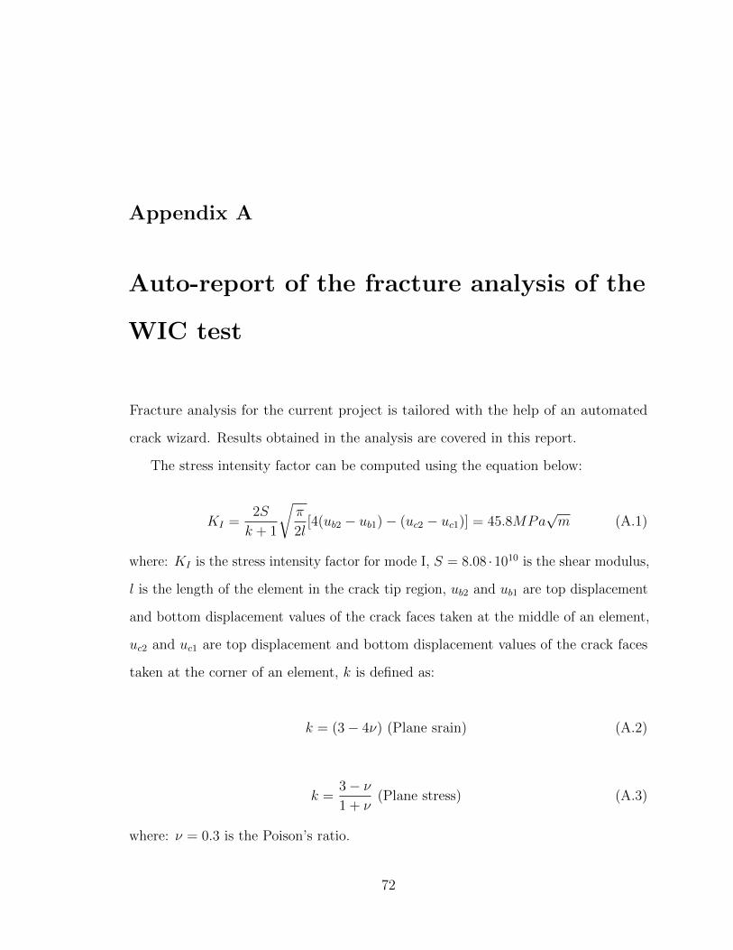
Appendix A

Auto-report of the fracture analysis of the

WIC test

Fracture analysis for the current project is tailored with the help of an automated

crack wizard. Results obtained in the analysis are covered in this report.

The stress intensity factor can be computed using the equation below:

KI =2S

k + 1

√π

2l[4(ub2 − ub1)− (uc2 − uc1)] = 45.8MPa

√m (A.1)

where: KI is the stress intensity factor for mode I, S = 8.08 ·1010 is the shear modulus,

l is the length of the element in the crack tip region, ub2 and ub1 are top displacement

and bottom displacement values of the crack faces taken at the middle of an element,

uc2 and uc1 are top displacement and bottom displacement values of the crack faces

taken at the corner of an element, k is defined as:

k = (3− 4ν) (Plane srain) (A.2)

k =3− ν1 + ν

(Plane stress) (A.3)

where: ν = 0.3 is the Poison’s ratio.

72

73

Now the result of the SIF can be compared to a known fracture toughness value.

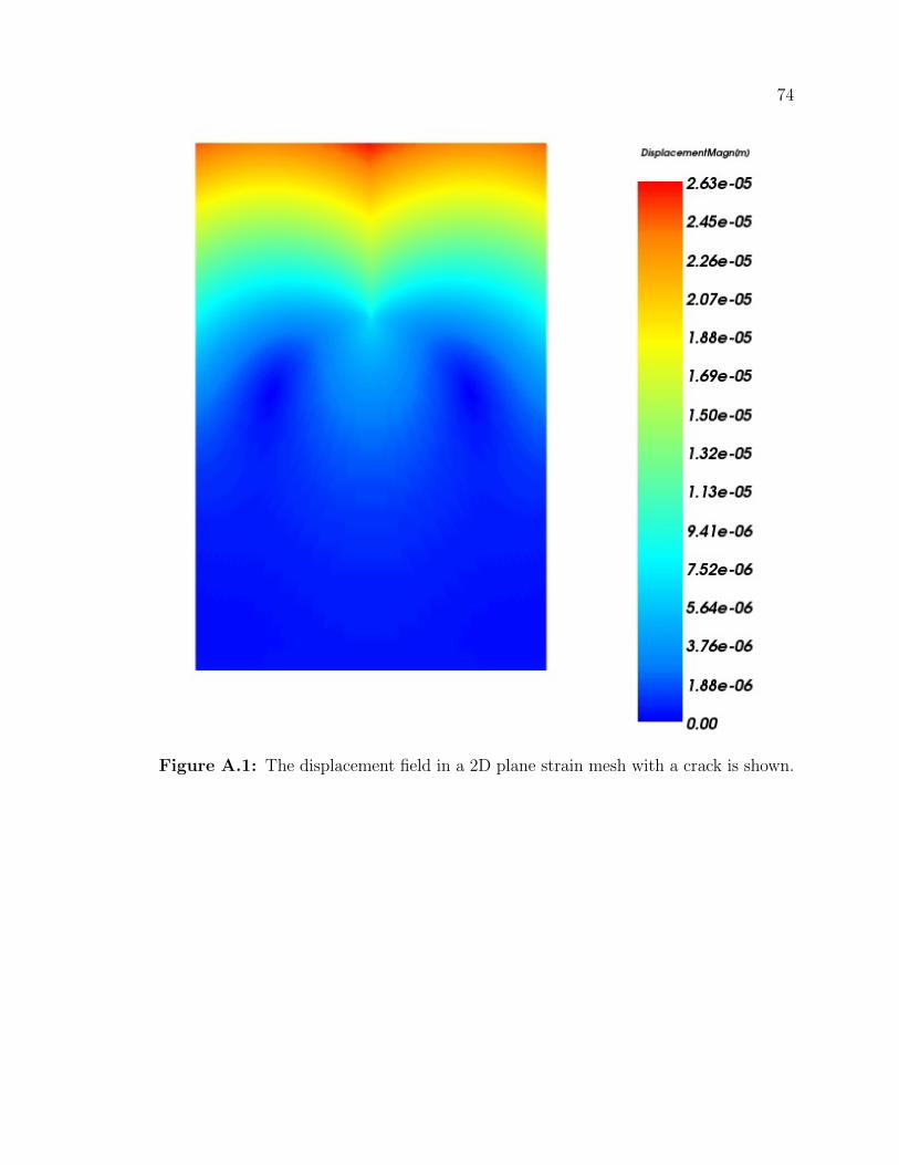
74

Figure A.1: The displacement field in a 2D plane strain mesh with a crack is shown.

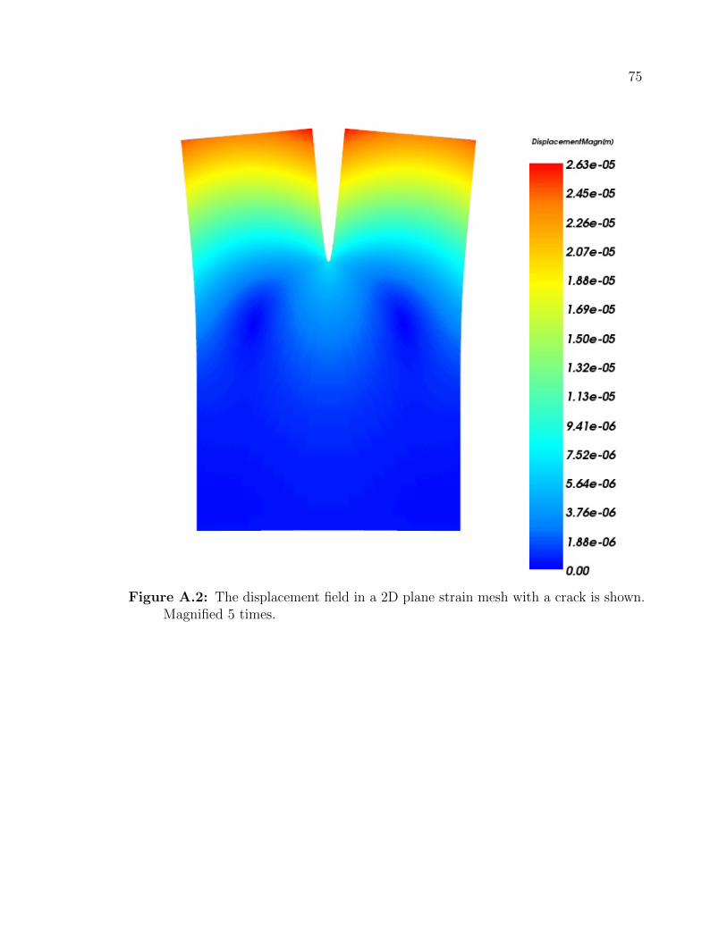
75

Figure A.2: The displacement field in a 2D plane strain mesh with a crack is shown.Magnified 5 times.

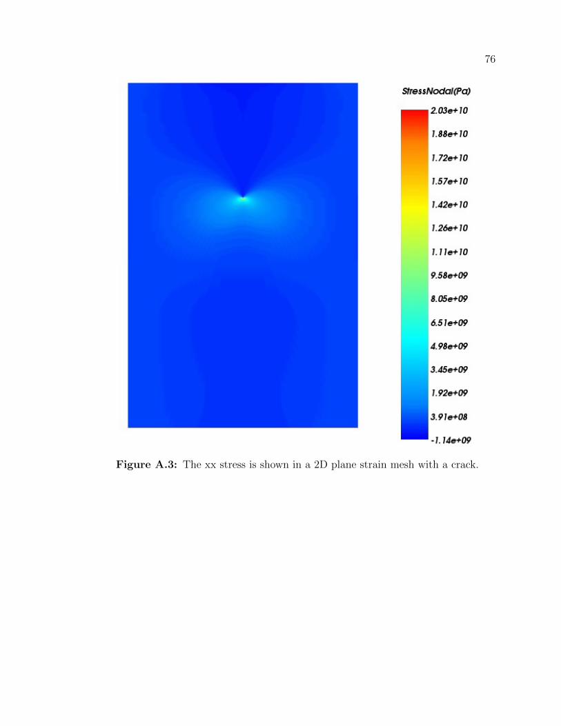
76

Figure A.3: The xx stress is shown in a 2D plane strain mesh with a crack.

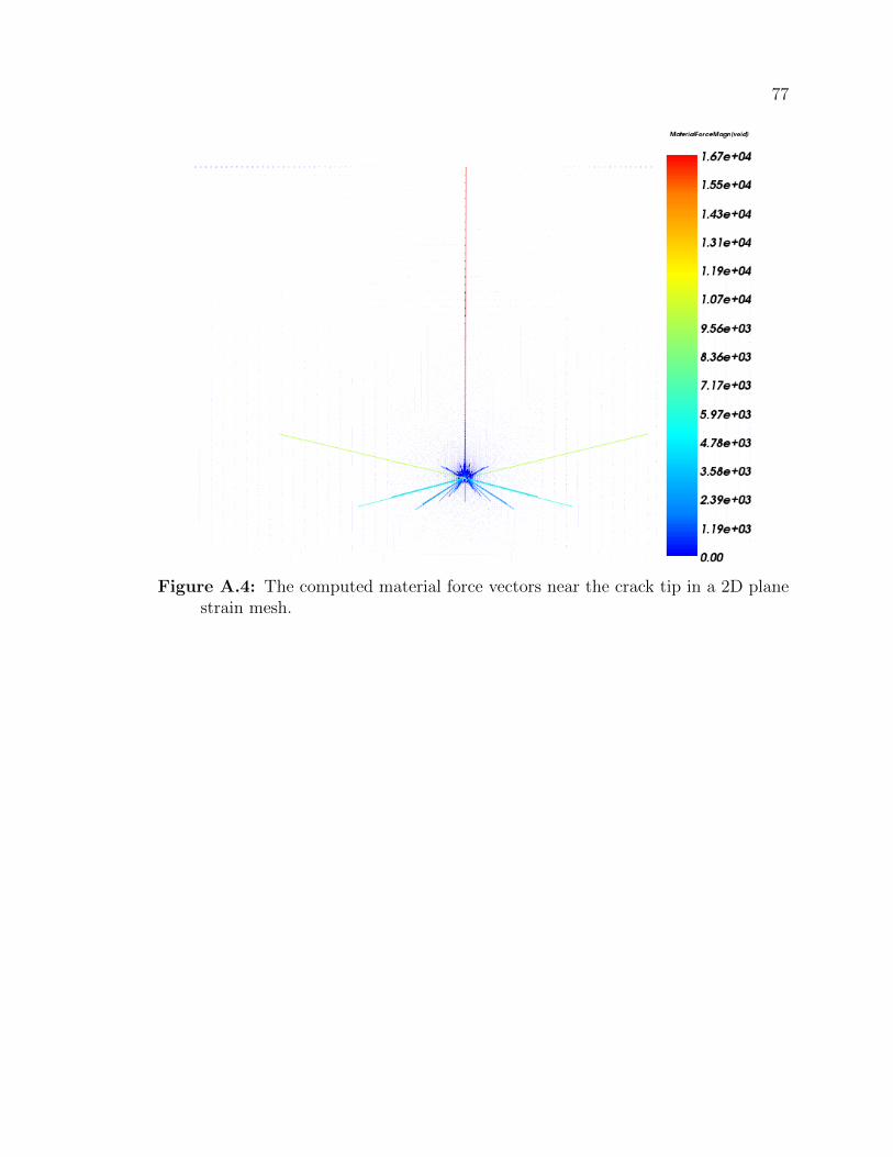
77

Figure A.4: The computed material force vectors near the crack tip in a 2D planestrain mesh.

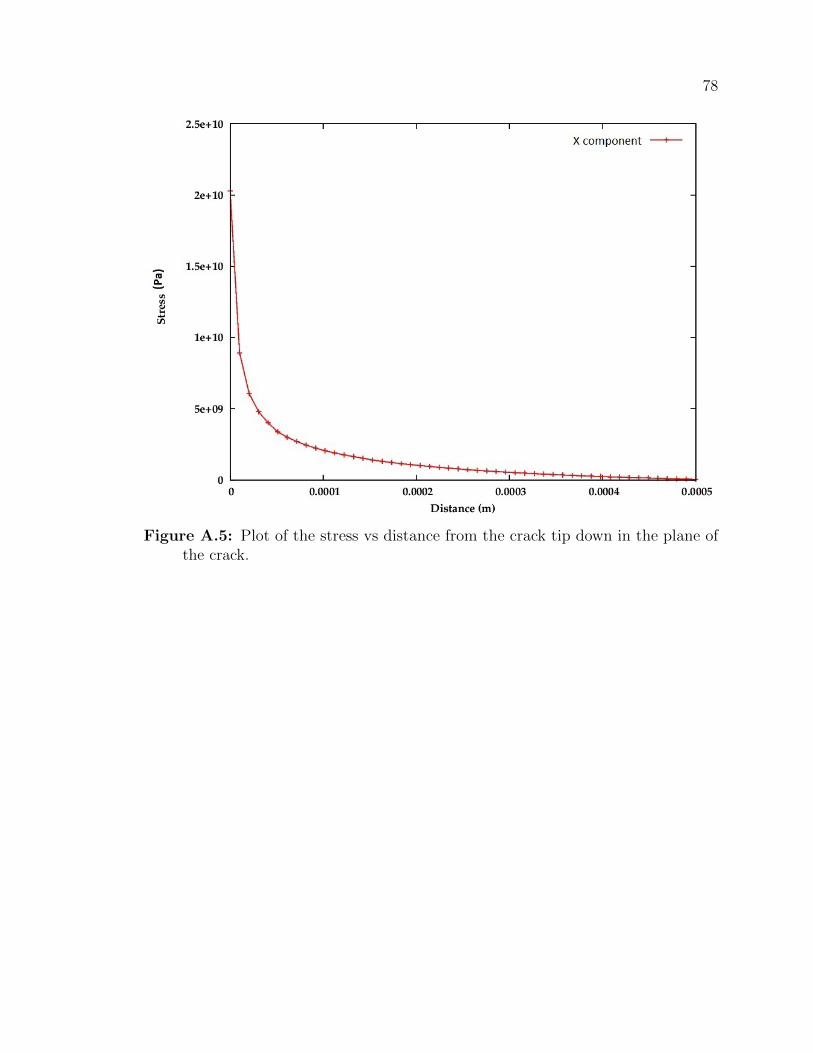
78

Figure A.5: Plot of the stress vs distance from the crack tip down in the plane ofthe crack.

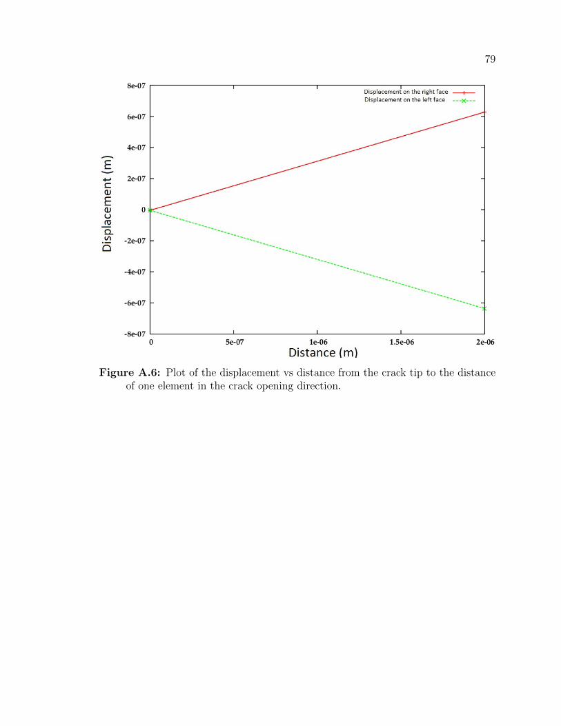
79

Figure A.6: Plot of the displacement vs distance from the crack tip to the distanceof one element in the crack opening direction.

Appendix B

Auto-report of the fatigue analysis of the

pipe girth weld for the crack length of 4

mm

Fatigue analysis for the current project is tailored with the help of an automated crack

wizard. Results obtained in the analysis are covered in this report.

The stress intensity factor can be computed using the equation below:

KI =2S

k + 1

√π

2l[4(ub2 − ub1)− (uc2 − uc1)] = 66.9MPa

√m (B.1)

where: KI is the stress intensity factor for mode I, S = 8.08 ·1010 is the shear modulus,

l is the length of the element in the crack tip region, ub2 and ub1 are top displacement

and bottom displacement values of the crack faces taken at the middle of an element,

uc2 and uc1 are top displacement and bottom displacement values of the crack faces

taken at the corner of an element, k is defined as:

k = (3− 4ν) (Plane srain) (B.2)

80

81

k =3− ν1 + ν

(Plane stress) (B.3)

where: ν = 0.3 is the Poison’s ratio.

The result of the SIF increment ∆K for the crack length of 4 mm can be used in

Paris-Erdogan equation.

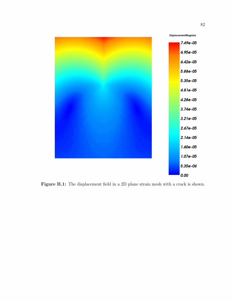
82

Figure B.1: The displacement field in a 2D plane strain mesh with a crack is shown.

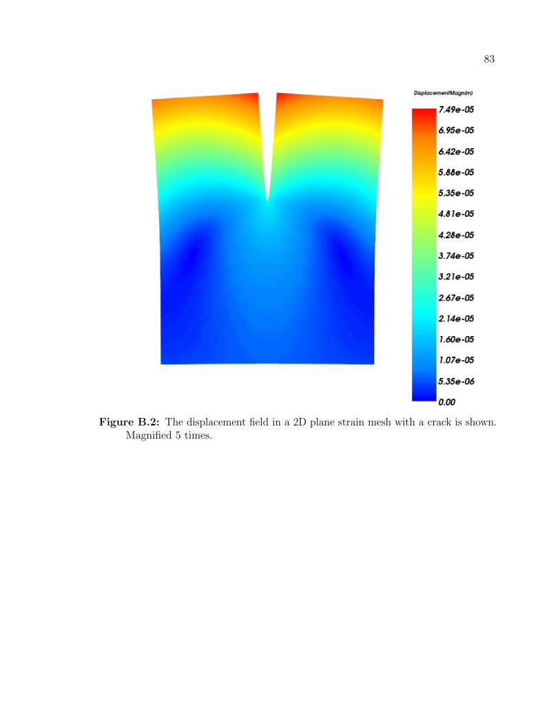
83

Figure B.2: The displacement field in a 2D plane strain mesh with a crack is shown.Magnified 5 times.

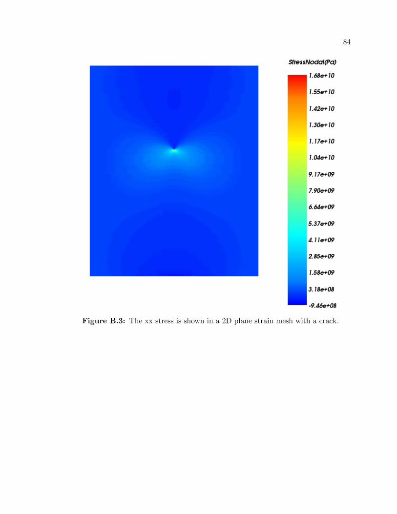
84

Figure B.3: The xx stress is shown in a 2D plane strain mesh with a crack.

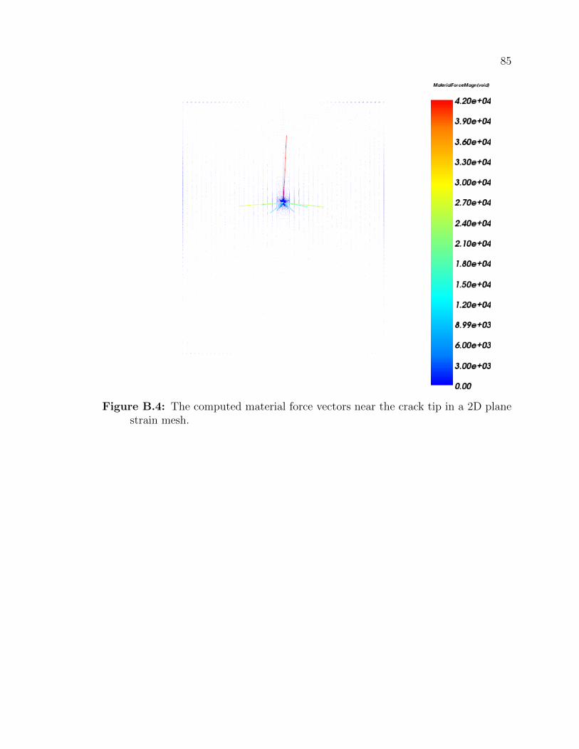
85

Figure B.4: The computed material force vectors near the crack tip in a 2D planestrain mesh.

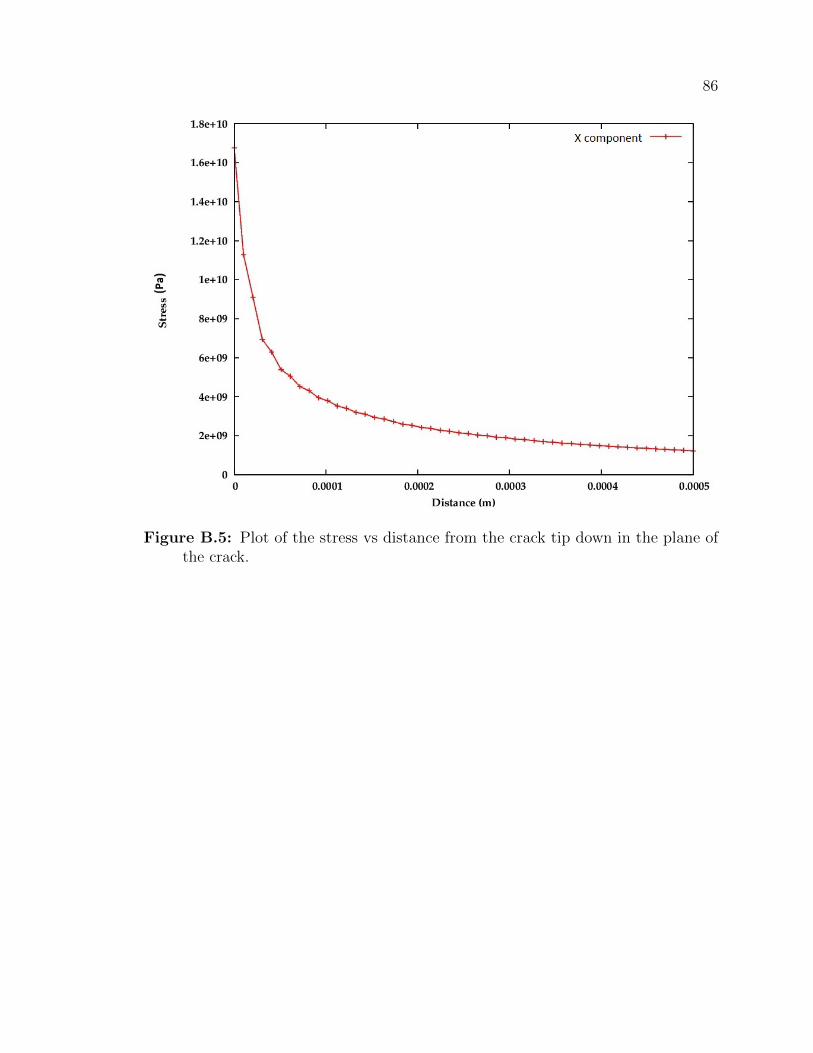
86

Figure B.5: Plot of the stress vs distance from the crack tip down in the plane ofthe crack.

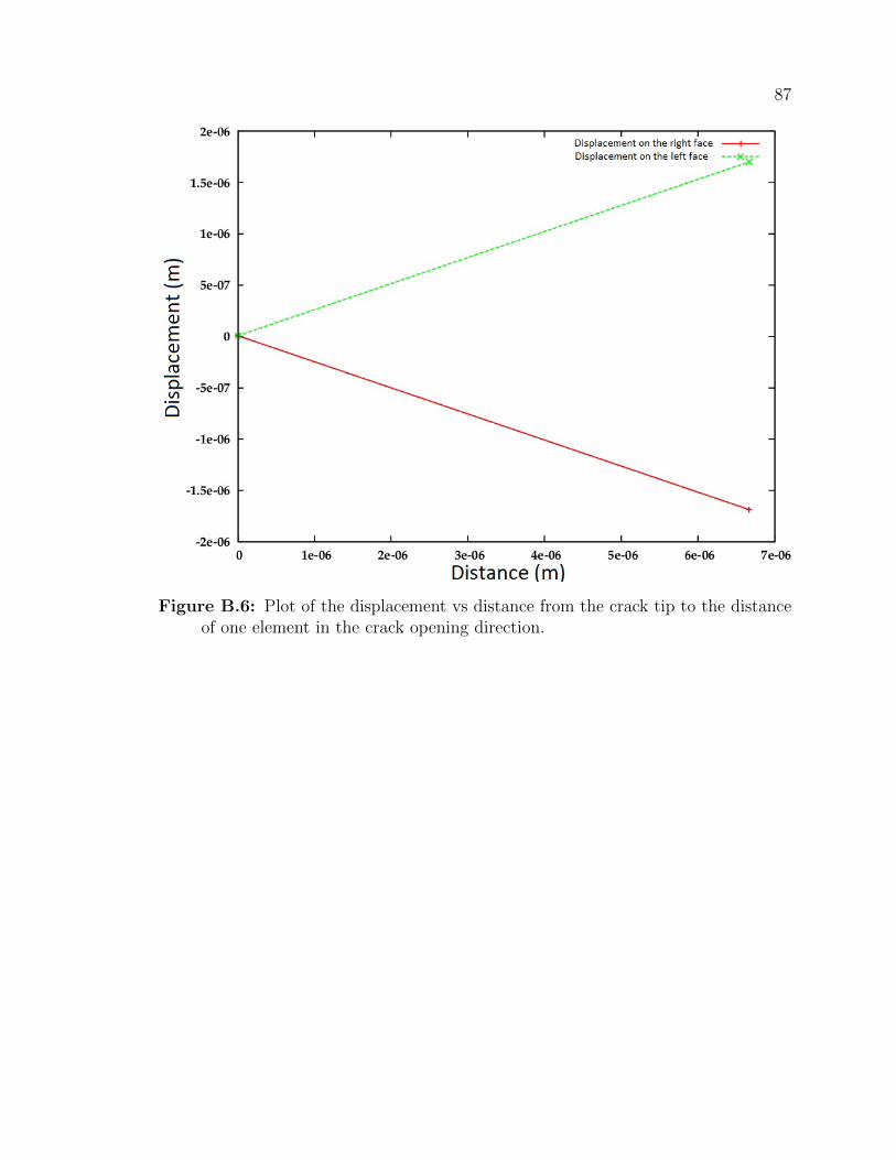
87

Figure B.6: Plot of the displacement vs distance from the crack tip to the distanceof one element in the crack opening direction.

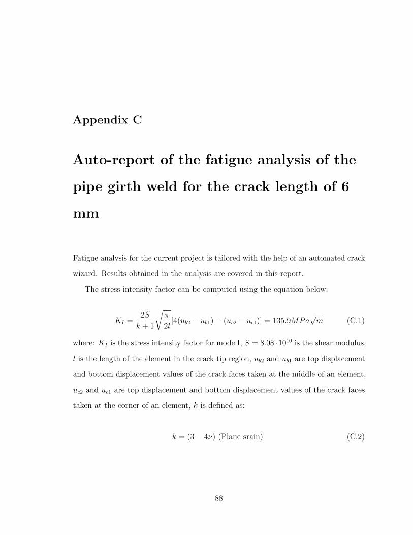
Appendix C

Auto-report of the fatigue analysis of the

pipe girth weld for the crack length of 6

mm

Fatigue analysis for the current project is tailored with the help of an automated crack

wizard. Results obtained in the analysis are covered in this report.

The stress intensity factor can be computed using the equation below:

KI =2S

k + 1

√π

2l[4(ub2 − ub1)− (uc2 − uc1)] = 135.9MPa

√m (C.1)

where: KI is the stress intensity factor for mode I, S = 8.08 ·1010 is the shear modulus,

l is the length of the element in the crack tip region, ub2 and ub1 are top displacement

and bottom displacement values of the crack faces taken at the middle of an element,

uc2 and uc1 are top displacement and bottom displacement values of the crack faces

taken at the corner of an element, k is defined as:

k = (3− 4ν) (Plane srain) (C.2)

88

89

k =3− ν1 + ν

(Plane stress) (C.3)

where: ν = 0.3 is the Poison’s ratio.

The result of the SIF increment ∆K for the crack length of 6 mm can be used in

Paris-Erdogan equation.

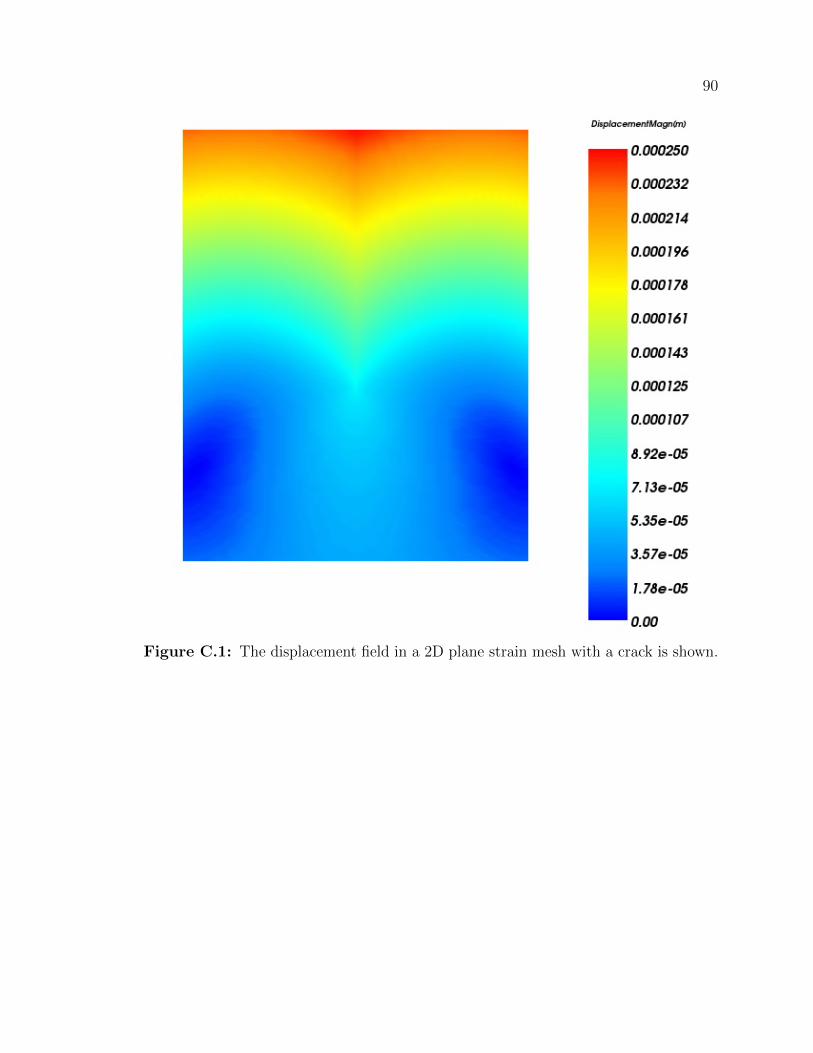
90

Figure C.1: The displacement field in a 2D plane strain mesh with a crack is shown.

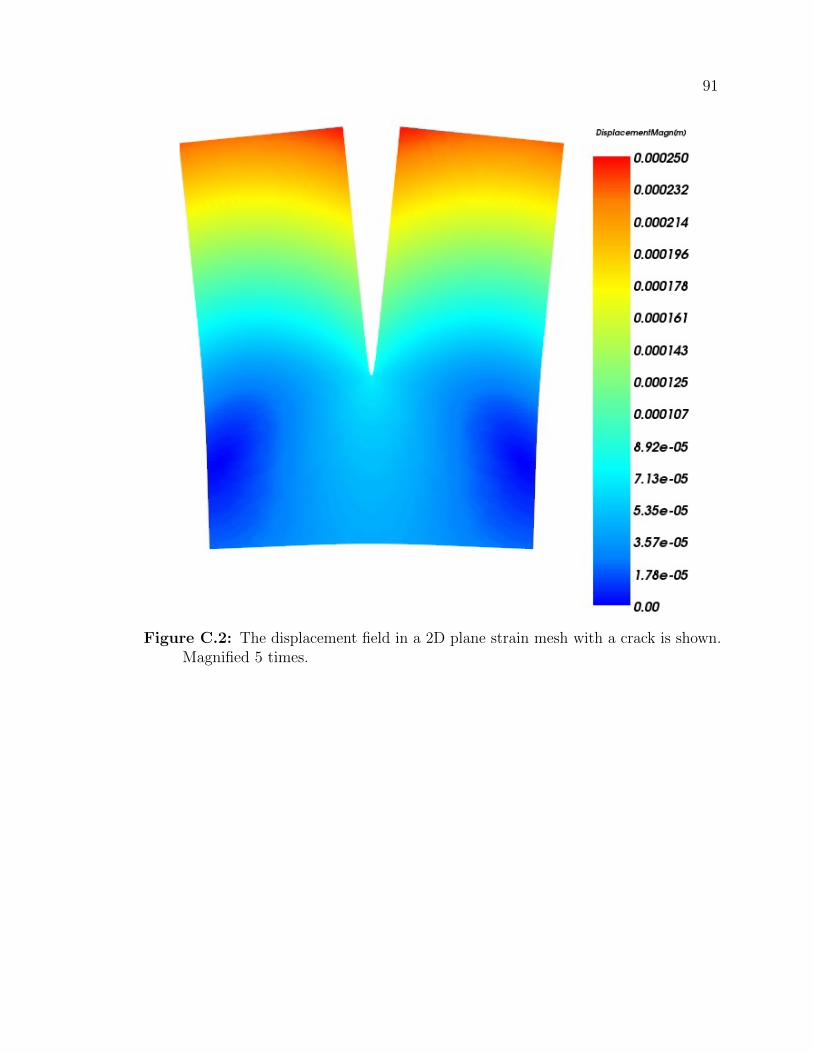
91

Figure C.2: The displacement field in a 2D plane strain mesh with a crack is shown.Magnified 5 times.

92

Figure C.3: The xx stress is shown in a 2D plane strain mesh with a crack.

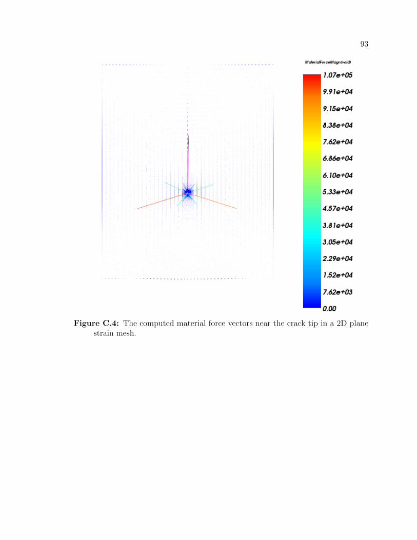
93

Figure C.4: The computed material force vectors near the crack tip in a 2D planestrain mesh.

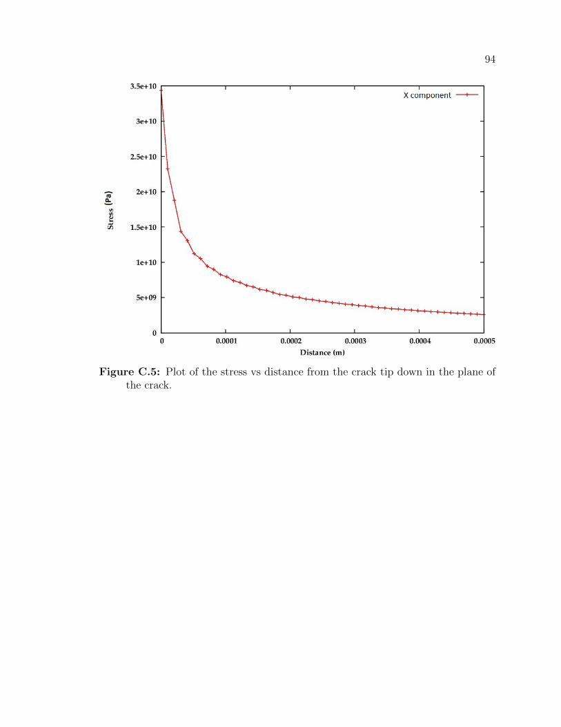
94

Figure C.5: Plot of the stress vs distance from the crack tip down in the plane ofthe crack.

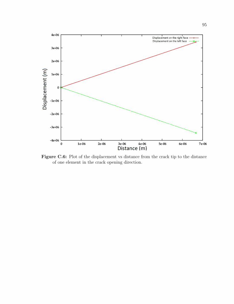
95

Figure C.6: Plot of the displacement vs distance from the crack tip to the distanceof one element in the crack opening direction.