HAL Id: hal-02309870https://hal.archives-ouvertes.fr/hal-02309870

Submitted on 10 Oct 2019

HAL is a multi-disciplinary open accessarchive for the deposit and dissemination of sci-entific research documents, whether they are pub-lished or not. The documents may come fromteaching and research institutions in France orabroad, or from public or private research centers.

L’archive ouverte pluridisciplinaire HAL, estdestinée au dépôt et à la diffusion de documentsscientifiques de niveau recherche, publiés ou non,émanant des établissements d’enseignement et derecherche français ou étrangers, des laboratoirespublics ou privés.

Algebras of coloured Petri netsFranck Pommereau

To cite this version:Franck Pommereau. Algebras of coloured Petri nets: and their applications to modelling and verifi-cation. LAP LAMBERT Academic Publishing, 2010, 978-3843361132. hal-02309870

Algebras of coloured Petri netsand their applications to modelling and verification

Franck Pommereau

September 2010

LAP LAMBERT Academic Publishing

ISBN: 978-3843361132

I

Acknowledgement. This books is my Habilitation thesis that was defended the 24th of

November 2009. I would like to thank warmly the reviewers, Pr. Eike Best (university of

Oldenbug, Germany), Pr. Serge Haddad (ENS Cachan, France) and Pr. Francois Vernadat

(INSA Toulouse, France), as well as the examiners, Pr. Didier Buchs (university of Geneva,

Switzerland), Pr. Hanna Klaudel (university of Evry, France), Pr. Elisabeth Pelz (university

Paris-East-Creteil, France) and Pr. Laure Petrucci (university Paris 13, France).

—Franck Pommereau

III

Table of Contents

1 Introduction . . . . . . . . . . . . . . . . . . . . . . . . . . . . . . . . . . . . . . . . . . . . . . . . . . . . . . . . . . . . . . . 5

1.1 Outlines . . . . . . . . . . . . . . . . . . . . . . . . . . . . . . . . . . . . . . . . . . . . . . . . . . . . . . . . . . . . . . . 7

2 A framework of composable Petri nets . . . . . . . . . . . . . . . . . . . . . . . . . . . . . . . . . . . . . . . . . 8

2.1 Preliminary definitions . . . . . . . . . . . . . . . . . . . . . . . . . . . . . . . . . . . . . . . . . . . . . . . . . . 8

2.2 Petri nets . . . . . . . . . . . . . . . . . . . . . . . . . . . . . . . . . . . . . . . . . . . . . . . . . . . . . . . . . . . . . . 9

2.3 Control flow operations . . . . . . . . . . . . . . . . . . . . . . . . . . . . . . . . . . . . . . . . . . . . . . . . . . 11

2.4 Synchronous communication . . . . . . . . . . . . . . . . . . . . . . . . . . . . . . . . . . . . . . . . . . . . . 15

2.5 Verification issues . . . . . . . . . . . . . . . . . . . . . . . . . . . . . . . . . . . . . . . . . . . . . . . . . . . . . . . 19

2.6 Related works . . . . . . . . . . . . . . . . . . . . . . . . . . . . . . . . . . . . . . . . . . . . . . . . . . . . . . . . . . 26

3 SNAKES toolkit and syntactic layers . . . . . . . . . . . . . . . . . . . . . . . . . . . . . . . . . . . . . . . . . . 28

3.1 Architecture . . . . . . . . . . . . . . . . . . . . . . . . . . . . . . . . . . . . . . . . . . . . . . . . . . . . . . . . . . . 28

3.2 Main features and use cases . . . . . . . . . . . . . . . . . . . . . . . . . . . . . . . . . . . . . . . . . . . . . . 29

3.3 A syntactical layer for Petri nets with control flow . . . . . . . . . . . . . . . . . . . . . . . . . . 30

3.4 Related works . . . . . . . . . . . . . . . . . . . . . . . . . . . . . . . . . . . . . . . . . . . . . . . . . . . . . . . . . . 33

4 Multi-threaded extension . . . . . . . . . . . . . . . . . . . . . . . . . . . . . . . . . . . . . . . . . . . . . . . . . . . . 35

4.1 Sequential fragment and exceptions . . . . . . . . . . . . . . . . . . . . . . . . . . . . . . . . . . . . . . . 35

4.2 Threading mechanism . . . . . . . . . . . . . . . . . . . . . . . . . . . . . . . . . . . . . . . . . . . . . . . . . . . 40

4.3 Use cases . . . . . . . . . . . . . . . . . . . . . . . . . . . . . . . . . . . . . . . . . . . . . . . . . . . . . . . . . . . . . . 43

4.4 Verification issues . . . . . . . . . . . . . . . . . . . . . . . . . . . . . . . . . . . . . . . . . . . . . . . . . . . . . . . 47

4.5 Related works . . . . . . . . . . . . . . . . . . . . . . . . . . . . . . . . . . . . . . . . . . . . . . . . . . . . . . . . . . 54

5 Applications . . . . . . . . . . . . . . . . . . . . . . . . . . . . . . . . . . . . . . . . . . . . . . . . . . . . . . . . . . . . . . . 56

5.1 Modelling time by causality . . . . . . . . . . . . . . . . . . . . . . . . . . . . . . . . . . . . . . . . . . . . . . 56

5.2 Specification and verification of security protocols . . . . . . . . . . . . . . . . . . . . . . . . . . . 61

5.3 Modelling biological regulatory networks . . . . . . . . . . . . . . . . . . . . . . . . . . . . . . . . . . . 68

6 Conclusion . . . . . . . . . . . . . . . . . . . . . . . . . . . . . . . . . . . . . . . . . . . . . . . . . . . . . . . . . . . . . . . . 77

6.1 Ongoing and future works . . . . . . . . . . . . . . . . . . . . . . . . . . . . . . . . . . . . . . . . . . . . . . . 78

5

1 Introduction

Formal specifications are now widely used for modelling systems and reasoning about them.

In particular, automated analysis through model-checking [28] is a successful approach that

involves different activities:

– a model of the system to analyse is defined, expressed in an adequate formalism;

– the properties to be verified against the model are specified, usually as logic formulas;

– the verification phase, or model-checking, consists in automatically determining whether the

properties hold or not for the defined model.

When the desired properties do not hold, the process often has to be started again: either the

model is correct and a flaw in the real system has been found, in which case the modelling

and verification process is likely to be restarted after the system is corrected; or the model

contains errors or is not precise enough and has to be fixed before the analysis is started again.

Even when the desired properties hold, some more details may often need to be added to the

model, different scenarios may be modelled or variants of the properties may be checked to

improve confidence in the obtained results. Modelling and verification are thus generally parts

of an incremental and cyclic process, either during the design phases of a system (used for

specification), or at a later point when the system exists (used for certification).

Among the numerous formalisms available for modelling, we concentrate here onto Petri nets

which are widely known and used in a variety of domains. Petri nets themselves exist in many

variants: from the basic model of places/transitions nets, or P/T nets [104], many extensions

have been proposed. We consider here the coloured Petri nets [67] variant that allows to cope

with high-level data types. In the field of formal modelling and verification, coloured Petri

nets are probably the most used formalism, together with timed automata [4]; as shown by the

incomplete and yet very long list of industrial case studies from the web pages of cpn tools [40].

One of the possible reasons for this success is that coloured Petri nets offer a set of modelling

devices that makes them easily applicable to a wide range of domains. In particular:

– like other Petri net models, coloured Petri nets naturally support the modelling of resources

consumption, production and sharing, access conflicts, concurrency and causal dependence,

locality, etc.;

– the concrete form of colours is a language; the richer it is, the easier the modelling task. In

particular, using a programming language for the colour domain makes it easy to model the

features from real-life examples, like computation involving complex data structures.

This results in a formalism offering a very good expressivity on two complementary aspects

that are linked to the essence of computing: control flow and data flow.

However, the weak point of Petri nets has been for a long time their lack of structuring

features: a Petri net is usually defined as a whole, not as a hierarchical system obtained by

assembling smaller blocks. This contrasts with the formalisms of the family of process algebras [9]

6

that exactly address the question of formalising compositionality: processes are composed at

a syntactical level and the behaviour of the compound is derived from the behaviour of the

components, depending on the operator that is used.

This lack has inspired the development of the Petri box calculus [11, 12] with the goal to fill

the gap between Petri nets and process algebras. The result is a family of Petri nets algebras

with full support for compositionally and a common approach to this aspect: a class of Petri

nets is considered and a special labelling is defined for it to provide all the information needed

for compositions; operators are then defined as transformations on Petri nets. The benefit from

this approach is that the result of a Petri net composition is still a regular Petri net (with labels)

and as such can be analysed using existing tools. Moreover, because it has been obtained in

a controlled way, some properties of a composed Petri net can be guaranteed by construction.

Not only does this relax from the need to verify these properties, but also they can be assumed

and exploited to improve further analyses.

The research presented in this document follows these principles. The purpose is to define

coloured Petri net formalisms with support for various features needed in practical situations; in

particular: explicit control flow, synchronous and asynchronous communication, exception and

threading mechanisms, functions (allowing recursion), and time-related capabilities. All this is

provided inside the domain of coloured Petri nets, with no extension of this base model that

would forbid to use the existing tools.

Moreover, we are concerned with the question of usability more than with the question

of expressivity: our formalisms should be easy to use and well suited for the modelling task

they were chosen for. To achieve this goal, we do not try to work toward the definition of a

thoroughly versatile formalism with all the possible features included. Instead, we prefer to offer

a flexible and modular framework allowing to easily define a suitable formalism for each specific

domain. Building a language with all included is not a difficulty in itself (see [112] for quite

a complete example), but the complexity of such a formalism is likely to discourage modellers

from learning it. Moreover, modelling power is almost always contradicting efficient verification:

in the domain of Petri nets for example, the complexity of many analysis problems increases

when more complex variants of Petri nets are considered, or the problems may even become

undecidable [52]. So, on the one hand, we aim at proposing formalisms that are specific to a

given usage or domain and, on the other hand, we shall exploit this specificity to accelerate

verification.

When a compromise has to be found between ease of modelling and speed of verification,

we try to consider the cyclic and incremental aspect of the modelling and verification process

as described above. Indeed, the amount of time spent in each cycle is composed of modelling

time spent by a human modeller, plus computation time spent by a program running on a

computer. Both matter and it is not worth restricting the modelling expressivity to speedup

verification if this is compensated for by a comparable modelling time penalty. Moreover, con-

sidering that computation time is comparatively cheaper than human time, especially that of

7

a highly-qualified modeller, it may be worth considering the trade-off the other way round: to

sacrifice some computation time for a simpler, faster and less error-prone modelling phase. Part

of the work presented hereby is directed toward this question and dedicated to propose devices

to improve modelling power while providing methods to preserve verification speed, or at least

to allow for reasonable efficiency.

Finally, to improve the suitability of formalisms, we shall consider hiding the Petri nets from

the modellers’ eyes and provide them with a syntax adapted to their domain and modelling

problems. Thus, Petri nets may be considered as the target domain for a compiler. This gives

an opportunity to really match the users’ needs, but also, this allows to limit the features

introduced at the Petri net level to primitive ones on the top of which the expected high-level

features can be implemented. Indeed, the modelling discipline and tedious steps to use these

primitives correctly can be hidden in the compilation process, as it is usual with most compiled

programming languages.

1.1 Outlines

In the next section, we present the core of a framework of composable Petri nets. It consists

in coloured Petri nets that can be equipped with labellings and operations to support control

flow and synchronous communication. These two aspects are presented separately but they are

compatible and may be used together. Then, we discuss the specific verification issues related

to the models presented in the section. Finally, a survey of related works is provided.

In section 3 we present the snakes toolkit that implements the presented models. Then,

in subsection 3.3, we illustrate how easily a simple yet rich syntax can be translated into Petri

nets thanks to the operations defined previously.

Section 4 defines an extension to the framework to support exceptions and threads. The

former is provided in the context of a sequential variant of the formalism defined in subsec-

tion 2.3: considering sequential processes is crucial to define a lightweight interrupt mechanism

on the top of which a fully-featured exception mechanism can be built. Then, this formalism

is extended with multi-threading to restore the possibility to model concurrent systems (in a

shape that is widely used in programming languages). A thread is here understood as a sequen-

tial process implemented as an identified flow of tokens in a Petri net. Threads can be started

dynamically and their termination can be awaited for. We then show how threads can be used

to model function calls. Introducing exception is harmless with respect to verification, but this

is not the case with threads. Indeed, adding thread identifiers increases the combinatorial ex-

plosion of the state space that may even become infinite. We show in subsection 4.4 how a

suitable state equivalence relation can be defined and efficiently computed in order to tackle

this issue. We end the section with a survey of related works.

Section 5 presents various applications of the formalisms presented in the previous sections.

In subsection 5.1 we discuss how time-related features can be modelled by causality: the idea

is to implement clocks by counters of occurrences of a tick transition; like for threads, this has

8

an important impact on verification and we show how this can be addressed. Then, in subsec-

tion 5.2, we apply the syntax introduced in subsection 3.3 to the modelling and verification of

security protocols. Finally, subsection 5.3 is a presentation of another application to the domain

of bio-informatics and, more precisely, to the modelling of regulatory networks used to analyse

patterning mechanisms in developmental processes. Each part of section 5 is provided with its

own survey of related works.

This document provides a uniformed version of various published research works. As a

consequence, some technical aspects have been simplified to streamline the presentation, but

full details may be found in the corresponding publications:

– section 2: [77, 108, 118, 43, 109, 44, 45, 110, 27, 112, 81];

– section 3: [114, 115, 107];

– section 4: [78–80, 112, 74, 76, 75]

– subsection 5.1: [111, 113, 110, 112, 117, 20];

– subsection 5.2: [107, 133];

– subsection 5.3: [29, 30].

2 A framework of composable Petri nets

2.1 Preliminary definitions

We shall use the lambda notation to denote some functions. For instance λ x : x > 0 denotes

the function that takes an argument x and returns the Boolean value x > 0. Similarly, function

λ x, y : x > y computes whether x is greater that y. If f and g are two functions on disjoint

domains F and G, we define f ∪ g as the function on domain F ∪ G such that (f ∪ g)|F = f

and (f ∪ g)|G = g.

A multiset m over a domain D is a function m : D → N (natural numbers), where, for

d ∈ D, m(d) denotes the number of occurrences of d in the multiset m. The empty multiset is

denoted by ∅ and is the constant function ∅ df= (λ x : 0). We shall denote multisets like sets with

repetitions, for instance m1df= 1, 1, 2, 3 is a multiset and so is d + 1 | d ∈ m1. The latter,

given in extension, is denoted by 2, 2, 3, 4. A multiset m over D may be naturally extended

to any domain D′ ⊃ D by defining m(d)df= 0 for all d ∈ D′ \D. If m1 and m2 are two multisets

over the same domain D, we define:

– m1 ≤ m2 iff m1(d) ≤ m2(d) for all d ∈ D;

– m1 +m2 is the multiset over D defined by (m1 +m2)(d)df= m1(d) +m2(d) for all d ∈ D;

– m1 −m2 is the multiset over D defined by (m1 −m2)(d)df= max(0,m1(d) −m2(d)) for all

d ∈ D;

– for d ∈ D, we denote by d ∈ m1 the fact that m1(d) > 0.

9

2.2 Petri nets

A (coloured) Petri net involves values, variables and expressions. These objects are defined

by a colour domain that provides data values, variables, operators, a syntax for expressions,

possibly typing rules, etc. For instance, one may use integer arithmetic or Boolean logic as colour

domains. Usually, more elaborated colour domains are useful to ease modelling, in particular,

one may consider a functional programming language or the functional fragment (expressions)

of an imperative programming language. In most of this document, we consider an abstract

colour domain with the following elements:

– D is the set of data values; it may include in particular the Petri net black token •, integer

values, Boolean values True and False, and a special “undefined” value ⊥;

– V is the set of variables, usually denoted as single letters x, y, . . . , or as subscribed letters

like x1, yk, . . . ;

– E is the set of expressions, involving values, variables and appropriate operators. Let e ∈ E,

we denote by vars(e) the set of variables from V involved in e. Moreover, variables or values

may be considered as (simple) expressions, i.e., we assume that D ∪ V ⊂ E.

We make no assumption about the typing or syntactical correctness of values or expressions;

instead, we assume that any expression can be evaluated, possibly to ⊥ (undefined). More

precisely, a binding is a partial function β : V→ D. Let e ∈ E and β be a binding, we denote by

β(e) the evaluation of e under β; if the domain of β does not include vars(e) then β(e)df= ⊥. The

application of a binding to evaluate an expression is naturally extended to sets and multisets

of expressions.

For instance, if βdf= x 7→ 1, y 7→ 2, we have β(x + y) = 3. With β

df= x 7→ 1, y 7→ "2",

depending on the colour domain, we may have β(x+ y) = ⊥ (no coercion), or β(x+ y) = "12"

(coercion of integer 1 to string "1"), or β(x + y) = 3 (coercion of string "2" to integer 2), or

even other values as defined by the concrete colour domain.

Two expressions e1, e2 ∈ E are equivalent, which is denoted by e1 ≡ e2, iff for all possible

binding β we have β(e1) = β(e2). For instance, x+1, 1+x and 2+x−1 are pairwise equivalent

expressions for the usual integer arithmetic.

Definition 1 (Petri nets). A Petri net is a tuple (S, T, `) where:

– S is the finite set of places;

– T , disjoint from S, is the finite set of transitions;

– ` is a labelling function such that:

• for all s ∈ S, `(s) ⊆ D is the type of s, i.e., the set of values that s is allowed to carry,

• for all t ∈ T , `(t) ∈ E is the guard of t, i.e., a condition for its execution,

• for all (x, y) ∈ (S × T ) ∪ (T × S), `(x, y) is a multiset over E and defines the arc from

x toward y. ♦

10

As usual, Petri nets are depicted as graphs in which places are round nodes, transitions are

square nodes, and arcs are directed edges. See figure 1 for a Petri net represented in both textual

and graphical notations. Empty arcs, i.e., arcs such that `(x, y) = ∅, are not depicted. Moreover,

to alleviate pictures, we shall omit some annotations (see figure 1): • for place types or arc

annotations, curly brackets around multisets of expressions on arcs, True guards, and node

names that are not needed for explanations. Finally, two opposite arcs may be represented by

a single double-arrowed arc, which occurs between s1 and t in the lower part of figure 1.

Ns1

t

x > 0

•s2x

x− 1

•S

df= s1, s2

Tdf= t

`df= s1 7→ N, s2 7→ •, t 7→ x > 0, (s1, t) 7→ x,

(s2, t) 7→ ∅, (t, s1) 7→ x− 1, (t, s2) 7→ •

Ns1

t

x > 0 s2x 7→ x− 1

Fig. 1. A simple Petri net, with both full (top) and simplified annotations (below).

For any place or transition x ∈ S∪T , we define •xdf= y ∈ S∪T | `(y, x) 6= ∅ and, similarly,

x•df= y ∈ S ∪ T | `(x, y) 6= ∅. For instance, considering the Petri net of figure 1, we have

•t = s1, t• = s1, s2, •s2 = t and s2• = ∅. Finally, two Petri nets (S1, T1, `1) and (S2, T2, `2)

are disjoint iff S1 ∩ S2 = T1 ∩ T2 = ∅.

Definition 2 (Markings and sequential semantics). Let Ndf= (S, T, `) be a Petri net.

A marking M of N is a function on S that maps each place s to a finite multiset over `(s)

representing the tokens held by s.

A transition t ∈ T is enabled at a marking M and a binding β, which is denoted by M [t, β〉,iff the following conditions hold:

– M has enough tokens, i.e., for all s ∈ S, β(`(s, t)) ≤M(s);

– the guard is satisfied, i.e., β(`(t)) = True;

– place types are respected, i.e., for all s ∈ S, β(`(t, s)) is a multiset over `(s).

If t ∈ T is enabled at marking M and binding β, then t may fire and yield a marking M ′

defined for all s ∈ S as M ′(s)df= M(s)− β(`(s, t)) + β(`(t, s)). This is denoted by M [t, β〉M ′.

The marking graph G of a Petri net marked with M is the smallest labelled graph such that:

– M is a node of G;

– if M ′ is a node of G and M ′[t, β〉M ′′ then M ′′ is also an node of G and there is an arc in

G from M ′ to M ′′ labelled by (t, β). ♦

It may be noted that this definition of marking graphs allows to add infinitely many arcs

between two markings. Indeed, if M [t, β〉, there might exist infinitely many other enabling

11

bindings that differ from β only on variables not involved in t. So, we consider only firings

M [t, β〉 such that the domain of β is vars(t)df= vars(`(t)) ∪⋃s∈S(vars(`(s, t)) ∪ vars(`(t, s))).

For example, let us consider again the Petri net of figure 1 and assume it is marked by

M0df= s0 7→ 2, s2 7→ ∅, its marking graph has three nodes as depicted in figure 2. Notice

that from marking M2, no binding can enable t because, either x 67→ 0 and then M2 has not

enough tokens, or x 7→ 0 and then both the guard x > 0 is not satisfied and the type of s1 is

not respected (x− 1 evaluates to −1).

M0 = s0 7→ 2, s1 7→ ∅

M1 = s0 7→ 1, s1 7→ •

M1 = s0 7→ 0, s1 7→ •, •

t, x 7→ 2

t, x 7→ 1

Fig. 2. The marking graph of the Petri net of figure 1.

2.3 Control flow operations

To define control flow compositions of Petri nets, we extend them with node statuses. Let S be

the set of statuses, comprising:

– e, the status for entry places, i.e., those marked in an initial state of a Petri net;

– x, the status for exit places, i.e., those marked in a final state of a Petri net;

– i, the status for internal places, i.e., those marked in intermediary states of a Petri net;

– ε, the status of anonymous places, i.e., those with no distinguished status;

– arbitrary names, like count or var , for named places.

Anonymous and named places together are called data or buffer places, whereas entry, internal

and exit places together are called control flow places.

Definition 3 (Petri nets with control flow). A Petri net with control flow is a tuple

(S, T, `, σ) where:

– (S, T, `) is a Petri net;

– σ is a function S → S that provides a status for each place;

– every place s ∈ S with σ(s) ∈ e, i, x is such that `(s) = •. ♦

Statuses are depicted as labels, except for ε that is not depicted. Moreover, we denote by

N e, resp. N x, the set of entry, resp. exit, places of N .

Let N1 and N2 be two Petri nets with control flow, we consider four control flow operations:

– sequential composition N1 #N2 allows to execute N1 followed by N2;

12

– choice N1 N2 allows to execute either N1 or N2;

– iteration N1 ~N2 allows to execute N1 repeatedly (including zero time), and then N2 once;

– parallel composition N1 ‖N2 allows to execute both N1 and N2 concurrently.

These operators are defined by two successive phases given below. The first one is a gluing

phase that combines operand nets; in order to provide a unique definition of this phase for all

the operators, we use the operator nets depicted in figure 3 to guide the gluing. These operator

nets are themselves Petri nets with control flow. The second phase is a named places merging

that fuses the places sharing the same named status.

e

i

x

t#1

t#2

e

x

t1 t2

e

x

t~1

t~2

e e

x x

t‖1 t

‖2

Fig. 3. Operators nets N#, N, N~ and N‖ (left to right). All the transition guards are True and all the depicted arcsare labelled by •.

Gluing phase The intuition behind this phase is that each transition of the involved operator

net represents one of the operands of the composition. The places in the operator net enforce

the correct control flow between the transitions. In order to reproduce this control flow between

the composed Petri nets, we have to combine their control flow places in a way that corresponds

to what specified in the operator net. For instance, let us consider N1 #N2. The corresponding

operator net is N# and let us call si its internal place. si is marked when t#1 has fired and this

marking allows t#2 to fire. At the level of composed nets, this should correspond to the fact that

N1 has finished its execution and so is in a final marking where all its exit places are marked;

at the same state, we should also have N2 in its initial marking where all its entry places are

marked. This can be obtained by combining the exit places of N1 (the net that will replace•si) with the entry places of N2 (the net that will replace si

•) through a Cartesian product.

From this example we can infer the gluing algorithm that consider in turn each place s of the

operator net and combine the exit places from the operand nets corresponding to •s with the

entry places from the operand nets corresponding to s•. An example is provided in figure 4.

Let ∈ #,,~, ‖ be a control flow operator and Ndf= (S, T, `) the corresponding

operator net. Let N1df= (S1, T1, `1, σ1) marked by M1 and N2

df= (S2, T2, `2, σ2) marked by M2

be two Petri nets with control flow such that N1, N2 and N are pairwise disjoint. In practice,

13

N1s1e

t1

s2x s3x

N2s4e s5e

t2 t3

s6x s7x

N1 #N2s1e

t1

t2 t3

s6x s7x

s2,4i s2,5i s3,4i s3,5i

Fig. 4. On the left: two Petri nets with control flow N1, N2. On the right: the result of the gluing phase of the sequentialcomposition N1 #N2. Place names are indicated inside places. Dotted lines indicate how control flow places are paired bythe Cartesian product during the gluing phase. Notice that, because no named place is present, the right net is exactlyN1 #N2.

nodes from N1 and N2 may be automatically renamed to enforce this condition. To simplify

the definition, for 1 ≤ i ≤ 2, we shall denote Ni by Nti and similarly for Si, Ti, `i and Mi.

We define the gluing of N1 and N2 according to as a Petri net with control flow (S, T, `, σ)

such that:

– for 1 ≤ i ≤ 2, for all t ∈ Ti, we also have t ∈ T with `(t)df= `i(t);

– for 1 ≤ i ≤ 2, for all s ∈ Si such that σi(s) /∈ e, x, we also have s ∈ S with `(s)df= `i(s),

σ(s)df= σi(s) and M(s)

df= Mi(s). Moreover, for all t ∈ Ti, we have `(s, t)

df= `i(s, t) and

`(t, s)df= `i(t, s);

– for every s ∈ S with s• = u1, · · · , un and •sdf= v1, · · · , vm, for every w

df= (e1, · · · , en,

x1, · · · , xm) ∈ N eu1× · · · ×N e

un ×N xv1× · · · ×N x

vm , there is a place sw in S such that:

• `(sw)df= `(s),

• σ(sw)df= σ(s),

• M(sw)df=∑

1≤i≤nMui(ei) +∑

1≤j≤mMvj(xj),

• for 1 ≤ i ≤ n, for all t ∈ Tui , `(t, sw)df= `ui(t, ei),

• for 1 ≤ j ≤ m, for all t ∈ Tvj , `(sw, t)df= `vj(xj, t);

– there is no other node nor arc.

Merging phase Let Ndf= (S, T, `, σ) be a Petri net with control flow marked by M . The

merging phase simply consists in merging together the places that have all the same named

status (i.e., not a control flow or anonymous status). This is illustrated in figure 5. This merging

resulting in the Petri net with control flow N ′df= (S ′, T ′, `′, σ′) marked by M ′ such that:

– T ′df= T and, for all t ∈ T , `′(t)

df= `(t);

14

– for all s ∈ S such that σ(s) ∈ e, i, x, ε, s is also a place in S ′ with `′(s)df= `(s), σ′(s)

df= σ(s)

and M ′(s)df= M(s);

– for all ς ∈ S \ e, x, i, ε, let Sςdf= s ∈ S | σ(s) = ς, if Sς 6= ∅, we add a place sς to

S ′ with `′(sς)df=⋃s∈Sς `(s), σ

′(sς) = ς and M ′(sς)df=∑

s∈Sς M(s); moreover, for all t ∈ T ,

`′(sς , t)df=∑

s∈Sς `(s, t) and `′(t, sς)df=∑

s∈Sς `(t, s);

– there is no other node nor arc.

e

x x

i i i i

•buffer

•buffer other

• ε

e

x x

i i i i••buffer

other

• ε

Fig. 5. On the left, a Petri net with control flow before the merging phase. On the right, named places have been merged.

Definition 4 (Control flow compositions). Let ∈ #,,~, ‖ be a control flow operator

and N the corresponding operator net. Let N1 marked by M1 and N2 marked by M2 be two

Petri nets with control flow such that N1, N2 and N are pairwise disjoint. Then, N1 N2 is

defined as the Petri net with control flow resulting from the gluing phase followed by the merging

phase. ♦

Named places are often used as buffers to support asynchronous communication, the sharing

of buffers between sub-systems is achieved by the automatic merging of places that share the

same name when the sub-systems are composed. In this context, we need a mechanism to specify

that a buffer is local to some sub-system. This is provided by the name hiding operation that

replaces a buffer name by ε thus forbidding further merges of the corresponding place. Name

hiding itself is a special case of a more general status renaming operation.

Definition 5 (Status renaming and name hiding). Let Ndf= (S, T, `, σ) be a Petri net with

control flow marked by M and let % be a partial function S \ e, i, x, ε → S \ e, i, x defining

the renaming of some statuses. Then, the status renaming operation, denoted N [%], results in

the Petri net with control flow defined as (S, T, `, σ′) and marked by M such that, for all s ∈ S:

σ′(s)df=

%(σ(s)) if % is defined on σ(s),

σ(s) otherwise.

Let ς ∈ S \ e, i, x, ε, the name hiding operation is defined as N/ςdf= N [ς 7→ ε]. ♦

15

Properties Some interesting properties of Petri nets with control flow can be established, refer

to [45, 81] for details.

First, let us call control-safe a Petri net with control flow whose control flow places remain

marked by at most one token under any evolution. Then, if two Petri nets are control-safe,

their composition by any of the control flow operations is also control-safe. This property

holds assuming a restriction about how operators may be nested. In particular, it should be

avoided to nest a parallel composition into an iteration, which leads to 2-bounded control flow

places instead of 1-bounded. We will see later on that such a restriction can be syntactically

enforced without loss of expressivity (see section 4). Such a property is interesting for verification

efficiency. In particular, it allows to efficiently compute unfoldings of Petri nets, or to introduce

optimisations at various stages of the computation of markings successors (see section 2.5).

Moreover, algebraic properties of the control flow operations can be established. In partic-

ular, if N1, N2 and N3 are two Petri nets with control flow and ς1, ς2 ∈ S \ e, i, x, ε, then we

have:

N1 N2 'N2 N1 commutativity of (N1 N2)N3 'N1 (N2 N3) associativity of

N1 ‖N2 'N2 ‖N1 commutativity of ‖(N1 ‖N2) ‖N3 'N1 ‖ (N2 ‖N3) associativity of ‖(N1 #N2) #N3 'N1 # (N2 #N3) associativity of #

N1/ς1/ς1 'N1/ς1 idempotence of /

N1/ς1/ς2 'N1/ς2/ς1 commutativity of /

(N1 ~N2)~N3 ' (N1 N2)~N3 equivalence of ~ and under ~

where ' is the equality of Petri nets up to nodes identities. The last property may be surprising

and stands more like a warning for the modeller to avoid mistakes. If this property is really

undesirable, the binary iteration may be replaced by a ternary iteration [N1 ∗N2 ∗N3] that is

equivalent to N1 # (N2 ~N3) and introduces a guard on the iteration N2 ~N3 through N1 [81].

2.4 Synchronous communication

Thanks to node statuses and the automatic merging of named places from composed Petri

nets, a form of asynchronous communication is possible. In this section, we consider an explicit

synchronous communication scheme based on transitions synchronisation, allowing to enforce

a simultaneous firing of sets of transitions with information exchange.

To specify how transitions may be synchronised, they are decorated with multi-actions,

i.e., multisets of actions. Let A be the set of actions names, an action is a term of the

form a!(e1, · · · , en) for a send action or a?(e1, · · · , en) for a receive action, where a ∈ A and

e1, . . . , en ∈ E. Intuitively, a send and a receive action with the same name correspond to a bi-

nary synchronisation if their parameters can be unified. An action with no parameter is denoted

without parentheses, as in a! or a?.

16

The operations described hereafter do not involve places and thus leave markings untouched;

so, we consider unmarked nets only, but the definitions can be trivially extended to marked nets.

Definition 6 (Petri nets with synchronisation). A Petri net with synchronisation is a

tuple (S, T, `, α) where:

– (S, T, `) is a Petri net;

– α is a function over T such that, for all t ∈ T , α(t) is a multi-action. ♦

Based on this labelling, we can define three operations:

– the synchronisation with respect to a ∈ A creates new transitions that model the simultane-

ous firing a set of transitions with pairs of unifiable actions a!(· · ·) and a?(· · ·);– the restriction with respect to a ∈ A removes all the transitions involving actions a!(· · ·) or

a?(· · ·);– the scoping with respect to a ∈ A is the synchronisation followed by the restriction: its

creates all the possible synchronisations and removes all the unsatisfiable ones.

Synchronisation We denote by x a tuple of parameters for a send or receive action, for

instance, action a!(1, y, z + 1) may be denoted as a!(x) with xdf= (1, y, z + 1). Let x and y be

two such tuples of parameters, an unifier γ of x and y is a partial function V → V ∪ D ∪ Esuch that γ(x) ≡ γ(y), where γ(e) denotes the substitution in e of the variables mapped by γ.

A send action a!(x) and a receive action a?(y) on the same name a are called conjugated if x

and y can be unified.

In general, if one unifier exists, there exist infinitely many others that can be obtained by

augmenting the domain, mapping variables to values instead of to variables, or choosing different

variables in the co-domain. In the following, we consider only one among the possible most

general unifiers, i.e., one that has a domain as small as possible and that do not map variables

to values as much as possible. For instance, x+y and z+1 can be unified by γ1df= x 7→ z, y 7→ 1,

but also by γ2df= x 7→ z, y 7→ 1, w 7→ 3, or γ3

df= x 7→ 1, y 7→ 1, z 7→ 1. Among γ1, γ2 and

γ3, only the former is a most general unifier. Notice that γ4df= z 7→ x, y 7→ 1 is another most

general unifier that could be used instead of γ1. As shown below, using any of the most general

unifiers is equivalent.

Intuitively, the synchronisation is obtained by creating new transitions from pairs of transi-

tions labelled with conjugated actions. The transition resulting from a binary synchronisation

is obtained by merging the two synchronised transitions, while unifying their variables and re-

moving the conjugated actions that allowed the binary synchronisation. This process of pairing

transitions is repeated until saturation. An example of a synchronisation is provided in figure 6.

Definition 7 (Synchronisation operation). Let Ndf= (S, T, `, α) be a Petri net with syn-

chronisation and a ∈ A be an action name. The synchronisation of N with respect to a, denoted

N sy a, is the Petri net with synchronisation N ′df= (S ′, T ′, `′, α′) defined as follows:

17

– S ′df= S and for all s ∈ S, `′(s)

df= `(s);

– `′ is ` extended on S ′ ∪ T ′ ∪ (S ′ × T ′) ∪ (T ′ × S ′) and α′ is α extended on T ′ as specified

below;

– T ′ is the smallest set of transitions such that T ⊆ T ′ and, for all t1, t2 ∈ T ′ such that there

is one action a!(x1) ∈ α(t1) and one action a?(x2) ∈ α(t2), and for every unifier γ of x1

and x2, there is a transition t′ ∈ T ′ with

• `′(t′) df= γ(`(t1) ∧ `(t2)),

• α′(t′) df= γ(α(t1)− a!(x1)+ α(t2)− a?(x2))

• for all s ∈ S, `′(s, t′)df= γ(`′(s, t1) + `′(s, t2)) and `′(t′, s)

df= γ(`′(t1, s) + `′(t2, s)). ♦

t1a!(x) x > 0 t2 a?(y), b!(y + z) t3 b?(w)

x z

y w

N0

t1a!(x) x > 0 t2 a?(y), b!(y + z) t3 b?(w)

x z

y w

t1,2

b!(x+ z)

x > 0

x z

xN1

df= N0 sy a

Fig. 6. Net N1 at the bottom is the result of the synchronisation with respect to a of net N0 at the top; t1 and t2 havebeen unified by γ

df= y 7→ x and merged as t1,2.

In this definition any most general unifier is acceptable because they all lead to transitions

that differ only by a renaming of their variables. Since variables are scoped to each transition

and its arcs, this makes no difference to rename them as far as it is made consistently in the

guard and the arcs (which is the case in the definition where we use the same unifier for the new

transition and its arcs). In general, to reduce the size of Petri nets, among a set of transitions

that are identical up to the renaming of their variables, all but one may be removed without

changing the behaviour in any essential way.

It may be noted that the definition above can lead to Petri nets with infinitely many transi-

tions. This is the case for instance in the Petri net depicted in figure 7. In practice this situation

can be avoided by forbidding a transition to be involved more than once in a synchronisation.

Restriction The restriction with respect to an action name simply consists in removing all the

transitions that involve this action name. An example of a restriction is provided in figure 8.

Definition 8 (Restriction operation). Let Ndf= (S, T, `, α) be a Petri net with synchroni-

sation and a ∈ A be an action name. The restriction of N with respect to a, denoted N rs a, is

the Petri net with synchronisation N ′df= (S ′, T ′, `′, α′) defined as follows:

18

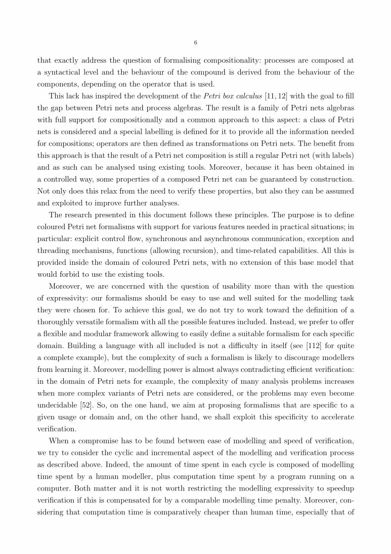
t1a?, a! t2 a?, a! t1a?, a! t2 a?, a!t1,2

a?, a!

Fig. 7. A binary synchronisation of t1 and t2 from the left net results in t1,2 in the right net. Transition t1,2 maythen be paired with either t1 or t2, resulting in transitions still labelled with multi-action a?, a!. So, a similar binarysynchronisation may be repeated at will.

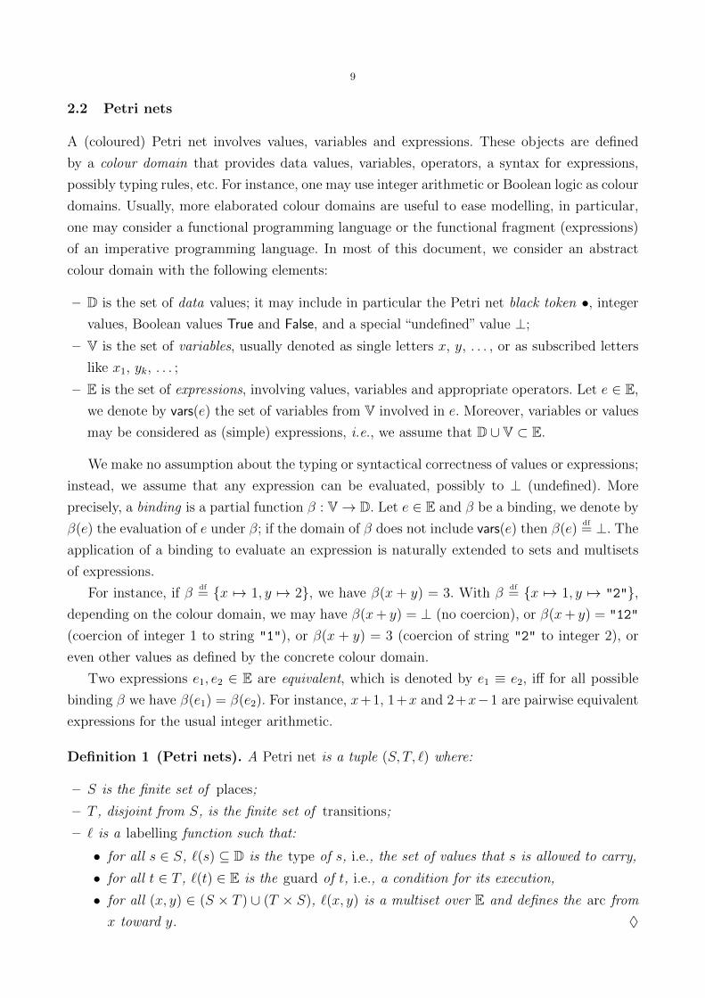
t3 b?(w)

w

t1,2

b!(x+ z)

x > 0

x z

xN2

df= N1 rs a

Fig. 8. The result of the restriction with respect to a of the net N1 from figure 6; transitions t1 and t2 (indicated indotted gray lines) have been removed.

– S ′df= S;

– T ′df= t ∈ T | a!(· · ·) /∈ α(t) ∧ a?(· · ·) /∈ α(t);

– `′ is ` restricted to S ′ ∪ T ′ ∪ (S ′ × T ′) ∪ (T ′ ∪ S ′);

– α′ is α restricted to T ′. ♦

Scoping The scoping operation is simply the successive application of the synchronisation and

the restriction. An example of a scoping is provided in figure 9.

Definition 9 (Scoping operation). Let N be a Petri net with synchronisation and a ∈ A be

an action name. The scoping of N with respect to a is N sc adf= (N sy a) rs a. ♦

t1,2,3 x > 0

x z

x x+ zN3

df= N2 sc b

Fig. 9. The result of the scoping with respect to b of the net N2 from figure 8; transitions t1,2 and t3 (indicated in dottedgray lines) have been unified by γ

df= w 7→ x+ z and merged as t1,2,3.

Properties An important property of Petri nets with synchronisation is that they can be

equipped for control flow (or, conversely, a Petri net with control flow can be equipped for

synchronisation). Indeed, control flow involves places while synchronisation involves transitions.

So, these extensions are orthogonal and perfectly compatible.

19

Like for control flow operations, algebraic properties of sc, sy and rs can be established. If

N is a Petri net with synchronisation and a1 , a2 ∈ A, then:

(N sy a1) sy a2 ' (N sy a2) sy a1 commutativity of sy

(N sy a1) sy a1 'N sy a1 idempotence of sy

(N rs a1) rs a2 ' (N rs a2) rs a1 commutativity of rs

(N rs a1) rs a1 'N rs a1 idempotence of rs

Moreover, considering Petri nets with both control flow and synchronisation, if % : S \ e, i, x, ε→ S \ e, i, x, we also have:

(N sy a1)[%]' (N [%]) sy a1 commutativity of sy and [·](N rs a1)[%]' (N [%]) rs a1 commutativity of rs and [·](N sc a1)[%]' (N [%]) sc a1 commutativity of sc and [·]

As a consequence, we also have the commutativity of synchronisation, restrictions and scoping

with buffer hiding.

2.5 Verification issues

In order to verify coloured Petri nets, the traditional approach has been expansion, i.e., trans-

lation from coloured to place/transition nets. This translation is often called unfolding but,

since this word is also used for MacMillan’s approach [86, 53], we use expansion instead. In this

approach, each possible token value in a place is converted into a p/t place and each possible

enabling binding of a transition is converted into a p/t transition, the arcs being connected

consistently. An example is provided in figure 10

•s

tx 6= y

21, 2, 3s′

3 2, 3s′′

•

x y

s•

tβ1 tβ2 tβ3 tβ4

s′1

•s′2 s′3 s′′2

•s′′3

β1df= x 7→ 1, y 7→ 2

β2df= x 7→ 1, y 7→ 3

β3df= x 7→ 2, y 7→ 3

β1df= x 7→ 3, y 7→ 2

Fig. 10. A coloured Petri net (on the left) and its expanded equivalent (on the right). The βi’s are the enabling bindingsof t in the coloured net as defined on the right part of the picture, the indexes of the places in the right net correspondto the values in the place types from the left net.

The main benefit from the expansion approach is that there exist many analysis techniques

and efficient tools dedicated to p/t nets. The problem in general is that the p/t net obtained

through expansion is too big and thus intractable; this net can even be infinite if there exist

coloured places with infinite types. A large or infinite type on a place does not mean that all

20

these values will be actually present in a reachable marking; in fact only a small subset of these

value is usually really reached. If this subset can be identified, expansion can be optimised by

reducing the number of p/t places and possible transitions enabling bindings. But very often,

this subset cannot be known in advance but only it can be discovered as the state space is

explored.

Fortunately, many tools exist to directly analyse coloured Petri nets, in particular [40, 94,

100, 70, 3, 5]. The main efficiency concern with this kind of tool is related to the colour domain:

the more general is the colour domain, the more difficult it is to perform fast analysis. In

particular, when computing the successors of a marking, the discovery of enabling bindings is

a time consuming process.

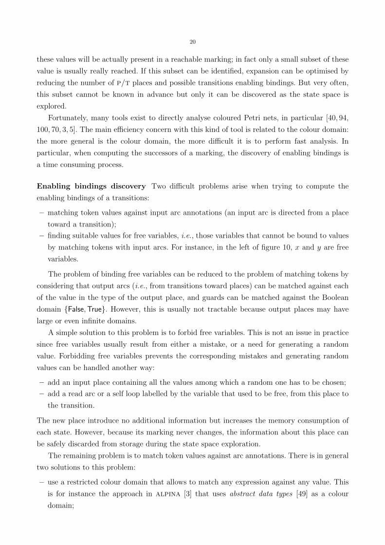
Enabling bindings discovery Two difficult problems arise when trying to compute the

enabling bindings of a transitions:

– matching token values against input arc annotations (an input arc is directed from a place

toward a transition);

– finding suitable values for free variables, i.e., those variables that cannot be bound to values

by matching tokens with input arcs. For instance, in the left of figure 10, x and y are free

variables.

The problem of binding free variables can be reduced to the problem of matching tokens by

considering that output arcs (i.e., from transitions toward places) can be matched against each

of the value in the type of the output place, and guards can be matched against the Boolean

domain False,True. However, this is usually not tractable because output places may have

large or even infinite domains.

A simple solution to this problem is to forbid free variables. This is not an issue in practice

since free variables usually result from either a mistake, or a need for generating a random

value. Forbidding free variables prevents the corresponding mistakes and generating random

values can be handled another way:

– add an input place containing all the values among which a random one has to be chosen;

– add a read arc or a self loop labelled by the variable that used to be free, from this place to

the transition.

The new place introduce no additional information but increases the memory consumption of

each state. However, because its marking never changes, the information about this place can

be safely discarded from storage during the state space exploration.

The remaining problem is to match token values against arc annotations. There is in general

two solutions to this problem:

– use a restricted colour domain that allows to match any expression against any value. This

is for instance the approach in alpina [3] that uses abstract data types [49] as a colour

domain;

21

– restrict the kind of annotations allowed on input arcs; for instance allowing only values or

variables allows for very simple matching or binding.

Restricting the colour domain is generally good for analysis capabilities and performances,

but usually bad for ease of modelling. For instance, abstract data types are expressive but

not always easy to use by an untrained modeller. On the other hand, restricting the kind of

annotations, when not done drastically, is rarely an issue in practice; in particular, we often

can transform Petri nets to remove input arcs labelled by expressions. For instance, assume

an arc from a place s toward a transition t labelled by an expression e. This arc label may

be replaced by a variable x /∈ vars(t) and the guard of t may be replaced by `(t) ∧ (x = e),

which usually produces the same result. This transformation is however not possible when

the evaluation of e has side effects. Fortunately, side effects are generally avoided as an error

prone programming practice; they are even impossible if the colour domain is a pure functional

programming language.

In snakes (see section 3), we have chosen to restrict annotations in a way which allowed

to have no restriction on the colour domain (full Python language). In cpn tools, annotations

of the input arcs have been restricted to what can be expressed with ml pattern-matching [67,

sec. 3.7]. Both snakes and cpn tools forbid free variables.

Compiling Petri nets Tools like [100, 5, 65] improve efficiency by compiling a Petri net into

machine code. The idea is to transform a Petri net into a library that provides all the primitives

to explore the state space of the compiled Petri net. For example, each transition can be compiled

into a function to discover enabling bindings at a given marking, plus a function to compute

the successor of a marking under a given binding. By using this approach, arc annotations and

guards are directly copied to the generated code, there is no need to interpret any of them

during analysis. In general, compilation avoids the need to continuously query complex data

structures (in particular the Petri net structure) throughout the computation. Notice that this

is possible only if the annotation language is also the target language of the compiler or can be

translated to it.

The code generated by the existing tools is rather generic in that it does not exploit any

information from the compiled Petri net other than what is strictly necessary. We propose

here to improve this approach by exploiting various information in order to optimise the code

generated by the compilation of a Petri net. In particular, the marking data structure can be

optimised for speed and memory consumption, which in turn allows to optimise algorithms

accordingly:

– in general, the tokens held by a place are stored in a multiset structure; but if the place has

singleton type x ⊂ D (in particular •), a counter of tokens is enough; moreover, if such a

place is known to be 1-bounded, then a Boolean is enough to record its marking; finally, the

marking of other 1-bounded places can be encoded with a single value in the place type, or

22

with ⊥. By compiling the Petri net, these optimisations are inlined in exploration algorithms

instead of being conditional branches of the code that handle the data structures;

– place invariants may be exploited to reduce the number of transitions examined during

state space exploration. Consider for instance a Petri net (S, T, `) and let I ⊆ S be a set

of places such that for all reachable marking M ,∑

s∈IM(s) = •. If a transition t fires

and puts a token • in a place s ∈ I, then, we known that all the transitions from (I \ s)•

are disabled because there cannot exist a token in another place in I. Moreover, transitions

from •s are also disabled since s cannot be marked by more than one token. In general, such

a 1-invariant I allows to build a generalised exclusion relation: the firing of a transition t

disables all the transitions in •(t• ∩ I)∪(I \ t•)•. If I can be computed statically, this conflict

relation can also be computed statically and exploited during the state space exploration to

avoid considering disabled transitions;

– token flows may be analysed to efficiently maintain a set of enabling bindings over the whole

Petri net. For instance, if a transition consumes but does not produce tokens from a place

s, then we known that this will remove enabling bindings for the transitions in s•. Similarly,

if tokens are added to s but none is removed, we known that this may add enabling binding

for the transitions in s•. Both these situations can be observed statically and the compiled

code can be optimised to take this into account.

A prototype implementation of these techniques has been developed and various examples

have been used as test cases, in particular some from the domain of security protocols (see

section 5.2 for such an example). By compiling various Petri nets, we could achieve speedups

ranging 6 to 10, depending on how many optimisations the models allowed us to introduce.

These speedups have been measured by comparing compiled nets with all the optimisations

disabled with respect to nets with all the optimisations allowed.

Exploiting structural information Providing structural information about the Petri nets

to analyse is usually either left to the user of a tool, or obtained by static analysis (e.g., place

invariants may be computed automatically). However, in our framework, Petri nets are usually

constructed by composing smaller parts instead of being provided as a whole. This is the case

in particular when the Petri net is obtained as the semantics of a syntax. In such a case, we

can derive automatically many structural information about the Petri nets.

For instance, when considering the modelling and verification of security protocols (see

section 5.2), systems mainly consist of a set of sequential processes composed in parallel and

communicating through a shared buffer that models the network. In such a system, we known

that, by construction, the set of control flow places of each parallel component forms a 1-

invariant. This property comes from the fact that the process is sequential and that the Petri

net is control-safe by construction. Moreover, we also know that control flow places are 1-

bounded, so we can implement their marking with a Boolean instead of an integer to count the

tokens as explained above. It is also possible to analyse buffer accesses at a syntactical level

23

and discover buffers that are actually 1-bounded, for instance if any access is always composed

either of a put and a get, or of a test, in the same atomic action.

Parallel computation The particular application to security protocols verification is also the

context of an ongoing PhD: the goal is to exploit the structure of these models to compute

efficiently the reachable states of a Petri net on a parallel computer. In order to guarantee

performances, the bulk synchronous parallel model of computation, BSP [131], is used. A bsp

program execution is composed of a succession of super-steps separated by synchronisation

barriers. This model of data parallelism enforces a strict separation of communication and

computation: during a super-step, no communication between the processors is allowed, only at

the synchronisation barrier they are able to exchange information. This execution policy has two

main advantages: first, it removes non-determinism and guarantees the absence of deadlocks;

second, it allows for an accurate model of performance prediction based on the throughput

and latency of the interconnection network, and on the speed of processors. This performance

prediction model can even be used online to dynamically make decisions, for instance choose

whether to communicate in order to re-balance data, or to continue an unbalanced computation.

In this context, the current work investigate the use of a fine tuned placement function

to distribute computed markings to the processors. Let h be a placement function to map any

marking to a processor number: for a marking M , h(M) is the number of the processor in charge

to compute the successors of M . Let G be the marking graph of the analysed Petri net and B

the spanning tree on G obtained from a breadth-first traversal. For two markings M1 and M2,

we define M1 < M2 iff M1 is an ancestor of M2 in B, and depth(M1)df= |M ′ s.t. M ′ < M1| is

the depth of M1 in B. We then define an equivalence relation over markings: M1 ∼M2 iff there

exist M ′1 and M ′

2 such that the following hold:

– h(M1) = h(M2);

– depth(M ′1) = depth(M ′

2);

– M ′1 ≤M1 and M ′

2 ≤M2;

– for 1 ≤ i ≤ 2, for all M such that M ′i ≤M ≤Mi we have h(M) = h(Mi).

Using this equivalence relation, we obtain G/∼ to coincide with the computation graph: each

class in G/∼ is a set of markings in G that can be computed during a super-step on a given

processor, without requiring a communication. For instance, we can use the following algorithm,

executed on each processor in parallel:

1| todo ← M0 if h(M0) = cpuid else # ‘‘cpuid’’ is the local CPU number2| seen ← 3| wait ← 4| total ← 15| while total > 0 :6| while todo 6= ∅ :7| choose M in todo

24

8| todo ← todo \ M9| seen ← seen ∪ M

10| for M ′ in successors(M) :11| if M ′ ∈ seen :12| continue # start next iteration of the for loop13| elif h(M ′) = cpuid :14| todo ← todo ∪ M ′15| else :16| wait ← wait ∪ M ′17| todo, total ← exchange(wait)

The algorithm starts by defining variables, locally to each processor. Line 1, each processor

defines a set of markings it has to proceed in the current super-step; initially, only one processors

has the initial marking M0, all the other are idle. Line 2, each processor defines the set of states

it knows, i.e., all those it has encountered during the computation. Line 3, variable wait is

defined to store all the states that have been computed by the processor but whose successors

have to be computed by another processor; these are the states waiting to be exchanged during

the next synchronisation barrier. Line 4, variable total is defined to store the total number of

markings exchanged at the last barrier. It is initially 1 because there is only one known marking

M0 (it was not exchanged however).

Then comes the main loop on line 5, that repeats until there is no more state to compute on

any processor, which is captured by variable total. Line 6, an inner loop allows each processor

to compute all it can without communicating with others. The computation is quite straight-

forward: each element in todo is proceeded in turn until exhaustion of todo; its successors are

computed (line 9) and added to todo if they must be proceeded locally (line 14), or to wait if

another processor should proceed them (line 16).

After this loop, line 17, all the awaiting data is exchanged during the synchronisation barrier

(triggered by the presence of a communication). Each state in wait is sent to the corresponding

processor according to h, and each processor receives a set of states to proceed and the number

of states exchanged during the barrier. If this number is zero, then the main loop has to be

stopped because all the processors are now idle.

So, a super-step corresponds to one execution of the main loop (except for the first super-

step that also executes lines 1–4). The set of markings computed by one processor during a

super-step corresponds exactly to one or several classes in G/∼ as illustrated in figure 11.

From this formalisation follow several observations, in particular:

1. The initial class of G/∼ should be as small as possible because the first super-step is highly

unbalanced.

2. Each class should be large enough to allow for many local computation.

3. In a breadth-first traversal of G/∼, each layer should have enough successors that should

be well distributed to ensure that the processors have a comparable amount of computation

to do.

25

super-step 0

super-step 1

super-step 2

processor 0 processor 1 processor 2

barrier 0

barrier 1

...

M0

......

...

Fig. 11. A possible computation graph of the parallel algorithm, assuming three processors 0, 1, 2 and h(M0) = 0. Thedepicted boxes denote classes in G/∼ (M0 is an element of the initial class). By definition of the algorithm, in super-step1, processor 0 is idle (it does not send work to itself).

To satisfy these expectations as much as possible, we can exploit the structure of the analysed

model to modify the placement function. In particular, h can be defined has a classical hash

on a subset H of places instead of on the whole marking. Consider a model consisting of n

sequential processes composed in parallel and communicating through shared places in a set

S0. Each sequential process i (for 1 ≤ i ≤ n) is defined by set of places Si in such a way that

the sets Sj (0 ≤ j ≤ n) form a partition of the places of the Petri net.

The ongoing work is about finding more criteria like those above and trying to derive rules

to ensure they can be fulfilled or at least not contradicted. For instance, from the items above,

we can derive:

1. H should contain the entry places of the sequential processes. Doing so, each transition fired

from M0 is likely to consume a token from one entry place and so to change class.

2. From the second item, it is clear that we should have H ∩ S0 = ∅: indeed, each time one

of the sequential process sends or receives a message, it produces or consumes a token on a

place from S0; if this place is in H then the new marking is in a new class. In communication

protocol, almost each transition involves sending or receiving a message, so, choosing H ∩S0 6= ∅ contradicts the second criteria.

3. H should be large enough or contain places with enough possible markings to allow for

enough hash values and thus to distribute work on all the processors.

26

Moreover, we investigate different algorithms following the same methodology but using

adapted definitions of ∼.

2.6 Related works

Coloured Petri nets are widely used in numerous variants: almost every tool that deals with

coloured Petri nets defines its own colour domain and its own restrictions on annotations.

Probably the most well known tool is cpn tools [40] and its model of ml-coloured Petri nets [67].

Another example of using a functional language is the model of Haskell-coloured Petri nets [124].

In general however, the colour domain is not an existing programming language but is defined

together with the analysis tool. For instance, Maria [94] and Helena [100] use a dedicated colour

domain that corresponds to data structures that they handle efficiently.

Supporting compositions of Petri nets is generally made by allowing to split a Petri net

into pages and hierarchies of modules, the union of which defining the whole system that is

obtained by fusion of the nodes present in several pages. This is more related to decomposition

than to composition of Petri nets, in an approach inspired from the splitting of programs

into separate files, modules and sub-programs. This approach is a practical requirement for a

modeller to be able to work directly at the Petri net level. Moreover it can be exploited for

modular verification [35, 87].

On the other hand, defining algebras of Petri nets is the domain of the Petri box calculus

family, pbc [11]. Unlike the previous one, this approach directly addresses compositions of

Petri nets and so is also applicable to define compositional Petri nets semantics of various

formalisms. The pbc is an algebra of p/t nets equipped with a process algebra syntax and

two fully consistent semantics: one is a denotational semantics given in terms of Petri nets,

the other is an operational semantics given in terms rewriting rules. The operators defined in

the pbc are those presented above: control flow and synchronous communication. The pbc has

been generalised later as the Petri net algebra, pna [12]. In parallel, the Petri net compositions

have been ported to coloured Petri nets, resulting in a model called M-nets [13], and a syntax

have been proposed for the M-nets [73]. M-nets rely for the definition of control flow on a very

general refinement operator that allows to substitute an arbitrary transition with an arbitrary

net [46]. This operation is well defined and really flexible but in practice leads to nets with

complex tree-shaped annotations and tokens, which cannot be handled efficiently during the

verification phase. This led to a series of models introducing in pbc the various high-level

features that exist in the M-nets. The asynchronous box calculus, abc [44, 43, 45], introduced

named places to support explicit asynchronous communication. Then, a variant with coloured

buffer places and parametrised synchronous communication have been introduced in [25, 27].

The abcd language presented in section 3.3 is a concrete implementation of the asynchronous

fragment of this last model. Numerous other variants of the pbc exist, in particular to model

timed systems, tasks and exceptions (see the related works surveyed in sections 4 and 5.1).

27

It is worth noting that not all the variants of the pbc are provided with an operational

semantics. This is indeed a features that used to exist to fill a gap between process algebras

and Petri nets but has never been really exploited: to the best of our knowledge, no analysis

method from the process algebra domain [9] has ever been ported to exploit pbc-like algebras.

This aspect has thus been left out of the present document that is focused toward providing

models that can be used for systems analysis, which still relies on the Petri net part of those

models.

There is a huge amount of literature about the questions around efficient verification of

Petri nets, this is partly due to the fact that there exist many variants of Petri nets. But this is

definitely a very active topic so we survey her only the works the most directly related to our

presentation. As already explained, the traditional verification approach through full expansion

is usually deprecated in favour of techniques that directly analyse coloured models. However,

Alpina [3] relies on partial expansion to perform structural analysis, and a tool like punf [70]

offers a smart alternative to expansion: punf can compute finite prefixes of coloured Petri nets

unfoldings, by producing just the p/t places that correspond to actually reached markings. So,

the result is much smaller than a full expansion. Moreover, the obtained unfoldings are symbolic

representations of the state space that can be directly analysed, usually achieving very good

compression in the presence of concurrency [86, 53, 71]. Moreover, if the model being unfolded

does not have auto-concurrency of transitions (this is the case with our models thanks to the

restrictions on the control flow), the so-called token swapping phenomenon [10] is avoided,

allowing a more efficient computation of the unfolding.

At the coloured level, the question of computing the reachable markings efficiently has been

addressed through various works about Maria [94], Helena [100] and cpn tools [40], and more

recently about asap [5]. Various techniques have been developed regarding various aspects of

the problem:

– efficient data structures in the colour domain with dedicated implementation on the verifi-

cation side allow to achieve both fast computation and low memory consumption [98, 97];

– the stubborn sets technique to reduce the state space by exploiting concurrency has been

ported to coloured Petri nets [58];

– modular verification and incremental state space construction allow generally to reduce both

memory usage and computation time by avoiding part of the combinatorial explosion that

arises in the whole system [87, 85, 72];

– techniques exist to lower memory requirement for the state space, either by storing it explic-

itly [96, 57], by keeping only required fragments [34, 83], by loosing information about it [64],

or by representing it symbolically using unfoldings [86, 53, 71] or decision diagrams [39, 61];

– the model itself may be reduced before to be analysed, while preserving its properties ob-

servable through verification [54, 55];

– compilation techniques have been used also in [95, 56], but without considering optimisations

of the generated code with respect to the compiled model.

28

Distributed computation has been used as well either to reduce computation time or to

increase storage capabilities. For instance, modular verification [101, 19] and unfolding [62] can

be distributed, and the technique to select a subset of place for hashing has been first intro-

duced in Spin model-checker [84]. However, these are distributed more than parallel algorithms.

The difference resides in that parallel computation relies on a model of parallelism, e.g., bsp

as presented above. This generally allows to achieve better scalability of algorithms when us-

ing hundreds or thousands of processors, or to predict an optimal number of processors for

a given computation. Indeed, increasing the number of processors for distributed algorithms

usually dramatically increase the amount of communication, which can quickly lead to amor-

tised speedup. Still, distributed algorithms are worth using on small clusters or local networks

of workstations, which are widely available and cheap configurations compared to specialised

parallel computers.

3 SNAKES toolkit and syntactic layers

snakes is a software library to define, manipulate and execute Petri nets [107]. A large part of

the work presented in this document have been implemented within snakes or using it.

snakes is a Python library that implements Python-coloured Petri nets. Python is a mature,

well established, interpreted language. According to its web site [120]:

Python is a dynamic object-oriented programming language that can be used for many

kinds of software development. It offers strong support for integration with other

languages and tools, comes with extensive standard libraries, and can be learned in a

few days. Many Python programmers report substantial productivity gains and feel the

language encourages the development of higher quality, more maintainable code.

It may be added that Python is free software and runs on a very wide range of platforms.

Python has been chosen as the development language for snakes because its high-level features

and library allows for quick development and easy maintenance, which is important considering

that snakes is maintained by only one person.1 The choice of Python as a colour domain then

became natural since Python programs can evaluate Python code dynamically. Moreover, if

Python is suitable to develop a Petri net library, it is likely that it is also suitable for Petri net

annotations.

3.1 Architecture

snakes is centred on a core library that defines classes related to Petri nets. Then, a set

of extension modules, i.e., plugins, allow to add features to the core library or to change its

behaviour. snakes is organised as a hierarchy of modules:

1 snakes is quite a large system, in its version 0.9.10 (July 2009), we could count in snakes around 100 classes and14000 lines of code, api documentation and unit tests.

29

– snakes is the top-level module and defines exceptions used throughout the library;

– snakes.data defines basic data types (e.g., multisets and substitutions) and data manipulation

functions (e.g., Cartesian product);

– snakes.typing defines a typing system used to restrict the tokens allowed in a place;

– snakes.nets defines all the classes directly related to Petri nets: places, transitions, arcs, nets,

markings, reachability graphs, etc. It also exposes all the api from the modules above;

– snakes.plugins is the root for all the extension modules of snakes.

The first four modules above (plus additional internal ones not listed here) form the core library.

snakes is designed so that it can represent Petri nets in a very general fashion:

– each transition has a guard that can be any Python Boolean expression;

– each place has a type that can be an arbitrary Python Boolean function that is used to

accept or refuse tokens;

– tokens may be arbitrary Python objects;

– input arcs (i.e., from places to transitions) can be labelled by values that can be arbitrary

Python object (to consume a known value), variables (to bind a token to a variable name),

tuples of such objects (to match structured tokens, with nesting allowed), or multisets of all

these objects (to consume several tokens). New kind of arcs may be added (e.g., read and

flush arcs are provided as simple extensions of existing arcs);

– output arcs (i.e., from transitions to places) can be labelled the same way as input arcs,

moreover, they can be labelled by arbitrary Python expressions to compute new values to

be produced;

– a Petri net with these annotations is fully executable, the transition rule being that of

coloured Petri nets: all the possible enabling bindings of a transition can be computed by

snakes and used for firing.

3.2 Main features and use cases

Apart from the possibility to handle Python-coloured Petri nets, the most noticeable other

features of snakes are:

– flexible typing system for places: a type is understood as a set defined by comprehension;

so, each place is equipped with a type checker to test whether a given value can be stored

or not in the place. Using module snakes.typing, basic types may be defined and complex

types may be obtained using various type operations (like union, intersection, difference,

complement, etc.). User-defined Boolean functions can also be used as type checkers;

– variety of arc kinds can be used, in particular: regular arcs, read arcs and flush arcs;

– support for the Petri net markup language (pnml) [106]: Petri nets may be stored to or

loaded from pnml files. In version 0.9.10 of snakes, only version 2.0 of pnml is supported:

snakes can export any net as xml, but this is valid pnml only for p/t nets;

– fine control of the execution environment of the Python code embedded in a Petri net;

30

– flexible plugin system allowing to extend or replace any part of snakes;

– snakes is shipped with a compiler that reads abcd specifications (see section 3.3) to pro-

duce pnml files or pictures;

– plugin gv allows to layout and draw Petri nets and marking graphs using GraphViz tool [51];

– plugin ops implements Petri nets with control flow as defined in section 2.3;

– plugin synchro implements Petri nets with synchronisation as defined in section 2.4;

– plugin query allows a program to invoke snakes remotely over a network connection by

exchanging pnml, this makes it possible for a non-Python program to use snakes;

– having Python-coloured Petri nets in a Python-programmed library makes it possible to

implemented the various features of the nets-within-nets paradigm [137] as shown in [116].

Finally, snakes has been used to implement various Petri nets related problems:

– the causal time calculus [110] is a timed pbc-like process algebra with a Petri net semantics

that has been implemented using snakes in less than 200 straightforward lines of code;

– boon [24] is an object-oriented programming notation with a Petri net semantics that has

been implemented using snakes from a Java program (over a network socket);

– a Petri net semantics of mins interconnection networks has been implemented and used for

simulation [103];

– a Petri net semantics of the security protocol language [41] has required also about 200 lines

of code;

– the compressed state space construction for Petri nets with causal time (presented in sec-

tion 5.1) have been implemented by combining snakes and Lash [17];

– security protocols have been specified and analysed using the abcd compiler and snakes

(see sections 5.2);

– the Petri net semantics of a formalism to model biological regulatory networks has been

implemented and examples have been studied using snakes (see section 5.3).

3.3 A syntactical layer for Petri nets with control flow

Considering our Petri nets as a semantics domain, it is possible to define languages adapted

to specific usages, with a well defined semantics given in terms of Petri nets. In order to

show how our framework makes this easy, we present now a syntax for Petri nets with control

flow that embeds Python programming language as colour domain. This language, called the

asynchronous box calculus with data, or ABCD, is a syntax for Petri nets with control flow where:

– the elementary (i.e., not composite) Petri nets are limited to simple ones like those depicted

in figure 12;

– the colour domain is the Python language.

abcd is a compromise between simplicity and expressiveness: not all the features available in

the framework are implemented (e.g., there is no synchronisation) but yet the language is useful

31

for many practical situations. In particular, abcd is well suited to specify modular systems

with basic control flow (including concurrency), and possibly complex data handling. This is

the case for many examples from the domain of computing; for instance, security protocols will

be addressed in section 5.2 while this section shows a simple railroad example.

An abcd specification is composed of the following elements:

1. A possibly empty series of declarations, each can be:

– a Python function declaration or module import: this corresponds to extensions of the

colour domain;

– a buffer declaration: a buffer corresponds to a named place in the semantics, thus buffers

are typed, unordered and unbounded;

– a sub-net declaration: this allows to declare a parametrised sub-system that can be

instantiated inside an abcd term.

2. A process term that plays the role of the“main”process: the semantics of the full specification

is that of this term (built in the context of the provided declarations). Process terms are

composed of atomic actions or sub-nets instantiations composed with the usual control flow

operators (but replaced with symbols available on a keyboard: ; for sequence, ∗ for iteration,

+ for choice and | for parallel). An atomic term is composed of a list of buffer accesses and

a guard. For instance:

– [True] is the silent action that can always be executed and performs no buffer access;

– [False] is the deadlocked action that can never be executed;

– [count−(x), count+(x+1), shift?(j), buf+(j+x) if x<10] is an atomic action that consumes

a token from a buffer count binding its value to variable x, produces a token computed as

x+1 in the same buffer, binds one token in a buffer shift to variable y without consuming

it, and produces the result of j+x in a buffer buf. All this is performed atomically and

only if x<10 evaluates to True.

The Petri net semantics of these three actions is depicted in figure 12.

A sub-net instantiation is provided as the name of the declared net block followed by the list

of effective parameters inside parentheses. The semantics of this instantiation is obtained by

substituting the parameters inside the definition of the sub-net and building its semantics

recursively. Then, the buffers declared locally to the sub-net are made anonymous using the

buffer hiding operator.

The semantics of a term is obtained by composing the semantics of its sub-terms using the

specified control flow operators. Finally, the semantics of a full specification also includes

the initial marking of entry and buffer places.

Like in Python, blocks nesting is defined through source code indentation only, and com-

ments start with character “#” and end with the line. Like in most compiled programming

languages (and unlike in Python), abcd has lexical scoping of the declared elements: an ele-

ment is visible from the line that follows its declaration until the end of the block in which it

is declared. As usual, declaring again an element results in masking the previous declaration.

32

[True]

e

True

x

[False]

e

False

x

[count−(x), count+(x+1), shift?(j), buf+(j+x) if x<10]

e

x < 10

x

count

intx 7→ x+ 1

shift

int

j

buf

int

j + x

Fig. 12. The Petri net semantics of various abcd atomic actions. The undirected arc attached to place shift is a readarc that binds j to a token but does not consume it upon firing.

Example As an illustration, let us consider a simple railroad crossing involving:

– one track on which trains can arrive repeatedly;

– one road crossing the track;

– a pair of gates to prevent cars to go on the track when a train is approaching;

– a red light to prevent the train to cross the road before the gates completely close.

When a train is approaching, a sensor on the track turns light to red and commands the gates

to go down. When they arrive down, the light is reset to green. When the train leaves the gates,

they are commanded to go up.

This system can be specified in abcd as follows. We first specify global buffers to model

the red light and a communication channel between the track and the gates:

1| # light is initially ”green”2| buffer light : in("red", "green") = "green"

3| # no command is available initially4| buffer command : in("up", "down") = ()

Keyword in used in the context of a buffer type definition specifies that this is an enumerated

type whose values are those provided inside parentheses as Python values. So, for instance,

buffer light can only hold the two strings "red" and "green" and initially contains "green".

Then we specify the behavior of the gates and provide for them an internal buffer allowing

to easily observe their current state.

5| net gates () :6| # gates are initially ”open”7| buffer state : in("open", "move", "closed") = "open"

8| # a sequence of actions9| (# receive command ”down” and start moving

10| [command−("down"), state−("open"), state+("move")] ;11| # finish to close and reset light to ”green”12| [state−("move"), state+("closed"), light−("red"), light+("green")] ;13| # receive command ”up” and start moving14| [command−("up"), state−("closed"), state+("move")] ;15| # finish to open16| [state−("move"), state+("open")])17| # this sequence is infinitely repeated because the loop exit cannot be executed

33

18| ∗ [False]

Then we specify the track on which trains can repeatedly arrive:

19| net track () :20| # we also need to observe if a train is crossing the road21| buffer crossing : bool = False22| # here also a sequence is infinitely repeated23| (# a train is approaching: light is turned red and gates are commanded to close24| [command+("down"), light−("green"), light+("red")] ;25| # the train must wait for green light before to go further and cross the road26| [ light?("green"), crossing−(False), crossing+(True)] ;27| # when the train leaves, gates are commanded to open28| [crossing−(True), crossing+(False), command+("up")])29| ∗ [False]

The full system is specified by running in parallel one instance of the gates and one of the

track.

30| gates() | track()

The semantics of this system is depicted in figure 13. We can notice that the buffers state and

crossing declared in sub-nets result each in an anonymous place: indeed, each has been hidden

during net instantiation, which takes place before the parallel composition, so the composition

could not merge these buffers. On the contrary, buffers command and light are globally declared

and thus result each in one merged named place.

This Petri net may be model-checked, for instance by searching a reachable state such that

the right-most anonymous place (i.e., buffer crossing from sub-net track) is marked by True

while the left-most anonymous place (i.e., buffer state from sub-net gates) is not marked by

"closed". Such a state would violate the basic safety condition: gates are closed whenever a

train is crossing the road. It can be checked that no such state is reachable with the current

model.

3.4 Related works

Several existing tools may be related in particular to snakes. The first one is the Petri net

kernel, pnk [125], that shares with snakes the aim to provide a general framework for building

Petri nets applications. The pnk provides a graphical user interface for editing and simulating

Petri nets. With respect to snakes, the basic model of the pnk is a less general model of

coloured Petri nets; however, this may be extended by writing Java code. Another difference is

that the pnk does not provide any of the operations to manage models from the pbc family,

which is of course not its aim. The development of the pnk does not appear to be active

anymore, the last release being dated of March 2002. The pnk is free software distributed

under the terms of the gnu gpl, which forces tools that use the pnk to be released under the

same licence. snakes uses gnu lgpl, which is less restrictive and allows to produce non-free

34

10

12

14

16•e

18False

opε

x

op 7→ mv

mv 7→ op

mv7→ cl

cl 7→mv

24

26

28

False

ε

• e

29 False

x

False 7→ True

True 7→ False

command"down"

"down"

"up"

"up"

"green"

light

"red"7→"green"

g:r

"green"

Fig. 13. The semantics of gates() | track(), where opdf= "open", cl

df= "closed", mv

df= "move" and g:r

df= ("green" 7→

"red"). The unlabelled places are internal ones. The anonymous place marked by op implements buffer state of net gates.The anonymous place marked by False implements buffer crossing of net track. Transition names correspond to the linenumbers of the atomic actions they implement.

software that uses snakes, but forces to release under the gnu lgpl any change made to

snakes.

Another tool with which snakes shares some goals is the Programming environment based

on Petri nets, pep [102]. The main similarity between the two tools is that both deal with

pbc and M-nets models. The main difference is that pep is oriented toward model-checking,

proposing a graphical user interface to define Petri net models through various ways. The Petri

nets variants in pep are fixed, mainly variants of pbc and a restricted version of M-nets; this

cannot be changed by users. pep also appears to be not maintained anymore, the last release

being dated of September 2004. pep was the tool we used before to decide to develop snakes.

The main reason for this decision was the impossibility to update pep quickly enough with

respect to theoretical developments in the pbc family, which is not surprising since pep was

never designed with this goal in mind. Like the pnk, pep is released under the gnu gpl.

Compared with cpn tools [40], snakes shares the ability to use a programming language for

nets inscriptions: a variant of ml for cpn tools, and Python for snakes. This makes it possible

to extend a lot the features of cpn tools. However, it does not provide support to introduce

another variant of Petri nets, for instance by changing the transition rule. So, there might be

new models of Petri nets that cannot be represented using one of those provided by cpn tools,

and thus for which the tools cannot be used. Another important difference is that cpn tools

is a end-user tool with an advanced graphical user interface while snakes is a programming

library. Finally, cpn tools is not open source.

35

More generally, since any Petri net modelled in snakes may be executed, it could be com-

pared with any Petri net tool that can simulate nets or compute their reachability graph.

However, executing nets is not the main purpose of snakes and it is not designed to do it

efficiently (even if it turns out to be satisfactory in many practical situations).

There exit many works dedicated to the translation of various syntax to Petri nets among

which essentially one can be directly related to abcd: the basic Petri net programming notation,

b(pn)2 [14, 108, 118, 80], aims at providing a syntax that is close to programming languages,

unlike abcd that is rather inspired by process algebra. b(pn)2 can be considered as more com-

plete than abcd with respect to its features, indeed, its latest extensions propose constructions

for procedures, tasks, exceptions and preemption. However, only procedures are implemented in

pep. On the other hand, abcd can be considered as a lightweight alternative whose semantics

produces more compact Petri nets. Both languages use the notion of atomic actions as the most

basic execution element. However, data in b(pn)2 is stored into variables instead of buffers; this

makes necessary to distinguish the value of a variable before the execution of an atomic action

from the value after its execution, denoted respectively by ′x and x′.

4 Multi-threaded extension

In this section, we present an extension to Petri nets with control flow to introduce two mod-

elling features: threads and exceptions. The former is modelled as the capability to execute

concurrently several instances of a sub-net, each being a sequential process. By restricting

parallelism to sequential threads running concurrently, it becomes possible to introduce in a

simple way an exception mechanism. Notice that this extension is compatible with Petri nets

with synchronisation. Notice also that exchanging parallel composition with threads does not

limit expressivity. Indeed, instead of a parallel composition N1 ‖ N2, it is possible to specify a

sequence like start(N2) # N1 # wait(N2) where start(N2) and wait(N2) are appropriate nets to

respectively start a new thread as an instance of N2 and wait for its termination. This results

in essentially the same behaviour.

To start with, we introduce the sequential fragment of the extension, defining Petri nets with

exceptions. On the top of this model, a new construct is added to support threading, leading to

define Petri nets with threads. In most of this section, we deal with unmarked Petri nets; this

will be justified when the elements to understand the reasons for this choice will be available.

At the end, we will see how to introduced markings again.

4.1 Sequential fragment and exceptions

We consider a model of Petri nets with exceptions, similar to Petri nets with control flow. The

main differences are that there is no parallel composition and that control flow places are now

coloured by two kind of tokens:

– black tokens • are used for regular control flow;

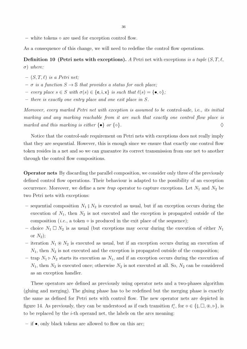
36

– white tokens are used for exception control flow.

As a consequence of this change, we will need to redefine the control flow operations.

Definition 10 (Petri nets with exceptions). A Petri net with exceptions is a tuple (S, T, `,

σ) where:

– (S, T, `) is a Petri net;

– σ is a function S → S that provides a status for each place;

– every place s ∈ S with σ(s) ∈ e, i, x is such that `(s) = •, ;– there is exactly one entry place and one exit place in S.

Moreover, every marked Petri net with exception is assumed to be control-safe, i.e., its initial

marking and any marking reachable from it are such that exactly one control flow place is

marked and this marking is either • or . ♦

Notice that the control-safe requirement on Petri nets with exceptions does not really imply

that they are sequential. However, this is enough since we ensure that exactly one control flow

token resides in a net and so we can guarantee its correct transmission from one net to another

through the control flow compositions.

Operator nets By discarding the parallel composition, we consider only three of the previously

defined control flow operations. Their behaviour is adapted to the possibility of an exception

occurrence. Moreover, we define a new trap operator to capture exceptions. Let N1 and N2 be

two Petri nets with exceptions:

– sequential composition N1 # N2 is executed as usual, but if an exception occurs during the

execution of N1, then N2 is not executed and the exception is propagated outside of the

composition (i.e., a token is produced in the exit place of the sequence);

– choice N1 N2 is as usual (but exceptions may occur during the execution of either N1

or N2);

– iteration N1 ~ N2 is executed as usual, but if an exception occurs during an execution of

N1, then N2 is not executed and the exception is propagated outside of the composition;

– trap N1 . N2 starts its execution as N1, and if an exception occurs during the execution of

N1, then N2 is executed once; otherwise N2 is not executed at all. So, N2 can be considered

as an exception handler.

These operators are defined as previously using operator nets and a two-phases algorithm

(gluing and merging). The gluing phase has to be redefined but the merging phase is exactly

the same as defined for Petri nets with control flow. The new operator nets are depicted in

figure 14. As previously, they can be understood as if each transition ti , for ∈ #,,~, ., is

to be replaced by the i-th operand net, the labels on the arcs meaning:

– if •, only black tokens are allowed to flow on this arc;

37

– if , only white tokens are allowed;

– it ?, both black and white tokens are allowed.

e

i

x

t#1

t#2

•

?

•

?

t1

t2

e

x

t1 t2

• •

? ?

t0

e

x

t~1

t~2

•?

t0

e

i

x

t.1

t.2

•

?

?

t1

t2

•

•

Fig. 14. Operators nets N#, N, N~ and N. (left to right). All transition guards are True.

Consider for instance the left most net, that specifies the sequence operator, and take N1 #N2

the sequential composition of N1 and N2. N# is started by putting one token in its entry place,

if this is •, transition t#1 and thus net N1 is executed. When it terminates, it produces a token

in the internal place. Again, if this is •, t#2 and thus N2 is executed until it puts a token in the

exit place. But, if N1 terminates with a token , indicating an exception during the execution

of N1, transition t2 is executed instead of t#2, which results in skipping N2 and propagating

the error until a trap. Similarly, if the net is started with in the entry place, this is directly

propagated to the exit place through transition t1. The situation is similar for the choice and

iteration operators. Consider now the trap operator net N.. It has the same structure as N# but

different tokens on the arcs after the internal place: here, if N1 terminates with •, this token is

directly propagated to the exit place; but if N1 produces , this token allows to execute t.2 and

thus N2, which is how the trap actually allows to capture exceptions. Notice that the arcs going

out of the transitions ti allow any token to be produced as the result of the execution of Ni.

In order to know how the labelling of arcs in an operator net influences the labelling of arcs

in the resulting nets, we define a function θ that maps a pair of arcs labels (in operator and

operand nets) to the label that has to be used in the resulting net. This function is defined by

the array depicted in figure 15.

Consider for instance transition t.1 in operator net N. and assume an operand net N1 that

has an entry places e with outgoing arcs to two transitions:

e•−−−−−−−−→ t1 and e

−−−−−−−−→ t2 .

When N1 is substituted to t.1, its place e becomes the entry place of the resulting net that also

includes t1 as well as t2. But the operator net allows only • to enter t.1 and thus to enter N1.

To enforce this, the labels of the arcs outgoing from e in the resulting net are computed using

38

operator label

operand label

m

∅

•

⊥

∅

⊥

•

•

⊥

∅

⊥

m

∅

•

?

∅

∅

∅

∅

∅

Fig. 15. The definition of θ, where m is a multiset over E that is neither •, nor ∅.

θ and we have:

eθ(•,•)−−−−−−−−−−−−−−−−−−−−−−−−−−−→ t1 =⇒ e

•−−−−−−−−→ t1 ,

eθ(•,)−−−−−−−−−−−−−−−−−−−−−−−−−−−→ t2 =⇒ e

⊥−−−−−−−−−−→ t2 .

So the arc to t1 is preserved because it is allowed while the arc to t2 is relabelled with ⊥. As

a result, t2 becomes a dead transition because ⊥ is not in the type of control flow places. So,

tokens introduced in e flow through the transition t1 (from N.) in the resulting net, which is

the expected behaviour. Because any token is allowed to flow out of t.1, the arcs to the exit place

of N1 is not changed (see the ? column in figure 15). Consider now transition t.2, substituted

with the same net N1. The result of applying θ is now:

eθ(,•)−−−−−−−−−−−−−−−−−−−−−−−−−−−→ t1 =⇒ e

−−−−−−−−→ t1 ,

eθ(,)−−−−−−−−−−−−−−−−−−−−−−−−−−−→ t2 =⇒ e

⊥−−−−−−−−−−→ t2 .

So, the precise meaning of the arc to t.2 is actually “take one token in the internal place and

start the net substituted to t.2”. So, a token is directly consumed by t1, i.e., by the transition

that corresponds to the regular starting of N1.

Gluing phase We can now define the new gluing phase. Compared with the previous definition,

the new one does not involve Cartesian products of entry or exit places because there is exactly

one of each in every Petri net with exceptions. Instead, a simple merging of the combined

places is enough to enforce the desired control flow. On the other hand, the definition takes into

account the use of θ and the presence of the additional transitions tj from the operator nets.

Let N1df= (S1, T1, `1) and N2

df= (S2, T2, `2) be two disjoint Petri nets with exceptions. Take

∈ #,,~, . and the corresponding operator net Ndf= (S, T, `) assumed disjoint from

both N1 and N2. Composition N1 N2 is Ndf= (S, T, `) defined as follows.

First, the nodes from N1 and N2 are copied to N , together with the arcs connecting them.

So, for 1 ≤ i ≤ 2, for all si ∈ Si and all ti ∈ Ti– si is also a place in S with `(si)

df= `i(si) and σ(si)

df= σi(si);

– ti is also a transition in T with `(ti)df= `i(ti);

– `(si, ti)df= `i(si, ti) and `(ti, si)

df= `i(ti, si).

The transitions of the operator net that are not replaced by a Ni are also copied to the resulting

net: for all t ∈ T \ t1, t2, we also have t ∈ T with `(t)df= `(t).

39

Finally, entry and exit places are combined to enforce the desired control flow. To do so, we

rely on the operator net N: we consider in turn all the places s of N and collect in a set P

the places originated from each Ni that should be merged and become the realisation of s in

the resulting net. So, for 1 ≤ i ≤ 2:

– if `(s, ti ) 6= ∅ then the entry place ei from Ni is added to P ;

– if `(ti , s) 6= ∅ then the exit place xi from Ni is added to P .

The places in P are merged, yielding a new place s whose label and status are that of s.

The last operation related to s is to adjust through θ the labelling of the arcs between s and

the transitions originated from each Ni; moreover, s has to be connected to the transitions

originated from N:

– for 1 ≤ i ≤ 2, for all ti ∈ Ti, and for all c ∈ N ei ∪ N x

i : `(s, ti)df= θ(`(s, ti ), `i(c, ti)) and

`(ti, s)df= θ(`(ti , s), `i(ti, c));

– for all t ∈ T \ t1, t2, `(s, t)df= `(s, t) and `(t, s)

df= `(t, s).

Optionally, the transitions in the resulting net having an incoming arc labelled by ⊥ can

be removed because they are dead transitions.

An exception mechanism What we have defined so far is a way to separate a regular control

flow from an exception control flow. However, this is not really an exception mechanism since

we cannot yet associate information to the occurrences of exceptions.

Usually, an exception is given a class (i.e., the exception type) and a value (e.g., a message);

however we can consider that this is just one arbitrary value. To store this information, each

Petri net with exception can be equipped with a data place named except whose type Err allows

to store the desired values. Using a single place is possible since a Petri net with exception is

sequential so there cannot occur more than one exception at the same time.

Then, to raise an exception associated with a value e ∈ Err , we can use the Petri net Re

depicted in figure 16. Its behaviour is very simple: when the transition fires, it changes the

regular control flow to exception control flow (i.e., consumes a black token in the entry place

and produces a white token in the exit place), while storing the exception value in place except.

e x

except Err

•

e

e

g(x)

x

except Err

• •

x

e

g(x)

x

except Err

•

x

Fig. 16. Left: net Re that raises an exception with value e ∈ Err . Middle: net Cg that catches an exception valueaccording to a Boolean function g. Right: net Pg that catches and propagates an exception value according to a Booleanfunction g.

The exception value stored in except is intended to be retrieved by an exception handler.

Most programming languages allow to select the exception to catch, usually according to its

40

type. Let us consider a Petri net N from which we want to catch exceptions e1 or e2 to trigger

handlers H1 and H2 respectively, while we want to let the other exceptions propagate to an

outer handler. This is possible by combining a trap to capture the error and a choice to select

the handler. Consider the Petri nets Cg and Pg depicted in figure 16, they are parametrised by

a Boolean function g that is used in the guards to accept or refuse an exception value. Using

these nets, our situation may then be modelled as:

N .((Cλx:x=e1 #H1) (Cλx:x=e2 #H2) Pλx:x/∈e1,e2

)

We can treat in a similar way the case where, instead of propagating an unknown exception,

we want to handle it using a net H:

N .((Cλx:x=e1 #H1) (Cλx:x=e2 #H2) (Cλx:x/∈e1,e2 #H)

)

4.2 Threading mechanism

We now define a model of Petri nets with threads that introduces various features allowing to:

– run concurrently multiple instances (threads) of a Petri net with exceptions;

– create (or spawn) threads dynamically;

– wait for threads termination;

– setup communication between threads through shared buffer places;

– check relationship between threads (parenthood, siblinghood, etc.);

– test whether a thread as terminated with an exception or not;

– implement function calls on the top of threads.

We call task a Petri that supports threads, i.e., a task is a Petri net from which separate

concurrent executions may be obtained. Each of this execution is a sequential process called a

thread. A task is thus a static object that is implemented as a Petri net (or part of a Petri net),

whereas a thread is a dynamic object that corresponds to tokens in the Petri net implementation

of a task. To distinguish tasks, each is assigned a task name from a set T. Similarly, to distinguish

threads, each is assigned a process identifier (or pid) from a set P.

A task is created from a Petri net with exceptions N and a task name task using a dedicated

operation denoted by Ltask : NM. This result in a Petri net with two distinguished places named

task .start and task .stop. A thread is created by putting a token into the place named task .start;

when it terminates its execution, it creates a token in the place named task .stop, this token

may be collected by another thread that is waiting for this termination. The two places named

task .start and task .stop play the same role for the task that the entry and exit places for the

corresponding Petri net with exceptions.

Finally, tasks may be combined using parallel composition, resulting in Petri nets with

threads. The relations between these various classes of Petri nets is illustrated in figure 17.

41

Lone : N1M Ltwo : N1M Lthree : N2M

N1 N2

e

x

e

x

one.start

one.stop

two.start

two.stop

three.start

three.stop

∥∥∥∥∥∥

∥∥∥∥∥∥

Fig. 17. The structure of the Petri net with threads framework. Boxes with plain line at the top represent Petri netswith exceptions N1 and N2, each depicted with its entry and exit place. Boxes with dashed lines at the bottom representtasks build from N1 and N2. Plain arcs show which task derives from which Petri net with exception. Dotted arcsindicate how entry (resp. exit) places in the Petri nets with exceptions are transformed into start (resp. stop) placesin the tasks. Finally, the large box with double line at the bottom represents the Petri net with threads obtained asLone : N1M ‖ Ltwo : N1M ‖ Lthree : N2M.

Petri nets with threads Tasks are named from the elements of T, these names are used

to build place names in order to be able to start a thread or wait for its termination. So, we

assume that, for all task ∈ T, we have task .start, task .stop ⊂ S \ e, i, x, ε.Running several instances of a Petri net could not be obtained by just putting several tokens

in its entry place because they would be all identical. Instead, we build the task so that every

place s of the original Petri net is copied to the task with the type P× `(s) in order to associate

each token to a pid. The arcs connected to these places are changed accordingly to pairs (π, x)

where π ∈ V is a reserved variable that can be interpreted as “my pid”. Some places should not

be changed: these are the non-anonymous data places that may be merged later on with those

from other tasks composed in parallel. These named places can be thought as external shared

resources used from within the task and, as such, not modified by the operation.

More precisely, let Ndf= (S, T, `, σ) be a Petri net with exceptions, Ltask : NM df

= (S ′, T ′, `′, σ′)

is defined as follows:

– T ′df= T and, for all t ∈ T ′, `′(t) df

= `(t);

– for every place s ∈ S such that σ(s) ∈ S \ e, i, x, ε, s is also a place in S ′ with `′(s)df= `(s)

and σ′(s)df= σ(s); moreover, for all t ∈ T ′, `′(s, t) df

= `(s, t) and `′(t, s)df= `(t, s);

42

– for every place s ∈ S such that σ(s) ∈ e, x, i, ε, there is a place s′ in S ′ with `′(s′)df= P×`(s)

and

σ′(s′)df=

task .start if σ(s) = e,

task .stop if σ(s) = x,

σ(s) otherwise;

moreover, for all t ∈ T ′, `′(s′, t) df= (π, x) | x ∈ `(s, t)) and `′(t, s′)

df= (π, x) | x ∈ `(t, s)).

The parallel composition of two disjoint nets N1df= (S1, T1, `1, σ1) and N2

df= (S2, T2, `2, σ2)

is denoted as usual by N1 ‖N2 and defined by applying the merging phase to net (S1 ∪S2, T1 ∪T2, `1 ∪ `2, σ1 ∪ σ2).

Definition 11 (Petri nets with threads). The class of Petri nets with threads is the small-

est class of Petri nets such that:

– if N is a Petri net with exceptions and task ∈ T, then Ltask : NM is a Petri net with threads;

– if N1 and N2 are Petri nets with threads then so is N1 ‖N2. ♦

As noted above, we are working with unmarked nets. Indeed, applying the task construction

to a marked net would raise the problem of choosing a thread to associate to the tokens. We

generally cannot know this in advance. Another choice would be to multiply the tokens so

that each possible thread can use its own copy. But this immediately produce large or infinite

markings: for each token value v, we would create the set of tokens P× v in the task. Since

none of these solution is satisfactory, we feel it is more reasonable to keep with unmarked net.

However, when a system is completely constructed, it consists in tasks in parallel. We can

choose one of the tasks as the main one and put a token in its start place: assuming that this

task is called main, the initial marking just has one token (π0, •) in the place named main.start,

where π0 is the pid of the initial thread.

Process identifiers Each thread is identified by a process identifier, or pid, from set P. We

assume that it is possible to check whether two pids are equal or not, since different threads

must be distinguished. Other operations may be applied to thread identifiers, in particular:

– π ^1 π′ holds iff π is the parent of π′ (i.e., thread π spawned thread π′ at some point of its

execution);

– π ^ π′ holds iff π is an ancestor of π′ (i.e., ^ is ^+1 );

– π t1 π′ holds iff π is a sibling of π′ and π was spawned immediately before π′ (i.e., after

spawning π, the parent of π and π′ did not spawn any other thread before spawning π′);

– π t π′ holds iff π is an elder sibling of π′ (i.e., t is t+1 ).

Throughout this section, we denote by Ωpid the set of the four relations introduced, as yet

informally, above together with the equality. (Note that other useful relations may be derived

from those in Ωpid .) In particular, only the operators in Ωpid can be used to compare pids in

the annotations used in Petri nets. Crucially, it is not allowed to decompose a pid (to extract,

43

for example, the parent pid of a given pid) which is considered as an opaque value (or a black

box). This implies, in particular, that no literals nor concrete pid values are allowed in Petri

net annotations (i.e., in guards and arc labels) involving the pids.

This formalism is very expressive while still decidable. Indeed, it can be shown that the

monadic second order theory of P equipped with ^1 and t1 can be reduced to a theory of

binary trees equipped with the left-child and right-child relation, which has been shown exactly

as expressive as tree automata [121]. However, many simple extensions of this formalism based

on pids (de)composition are undecidable.

We assume that there exists a function ν(π) that generates the next child of the thread iden-

tified by a pid π. There is no other way to create a thread’s pid. A possible way of implementing

dynamic pids creation—adopted here—is to consider them as finite sequences of positive inte-

gers: for all π, let i be the count of threads already spawned by π, set ν(π)df= π.(i + 1) (i.e.,

we write down the pids as dot-separated sequences). To be able to correctly implement ν, each

thread is assumed to maintain a count of the threads it has already spawned. Then the relations

in Ωpid other than equality are given by:

π ^1 π′ ⇐⇒ ∃i ∈ N+ : π.i = π′

π ^ π′ ⇐⇒ ∃n ≥ 1,∃i1, . . . , in ∈ N+ : π.i1. · · · .in = π′

π t1 π′ ⇐⇒ ∃π′′ ∈ P,∃i ∈ N+ : π = π′′.i ∧ π′ = π′′.(i+ 1)

π t π′ ⇐⇒ ∃π′′ ∈ P,∃i < j ∈ N+ : π = π′′.i ∧ π′ = π′′.j

Such a scheme has several advantages: (1) it is deterministic and allows for distributed

generation of pids; (2) it is simple and easy to implement and there is no reuse of pids; and

(3) it may be bounded by restricting, e.g., the length of the pids, or the maximum number of

children spawned by each thread. To implement ν, each thread has to maintain a counter of its

children. This can be made in a global place named pidcount and typed by P×N+: each token

(π, i) in this place records that the thread identified by π has spawned i children so far. The

next child spawned by π will thus receive pid π.(i+ 1). Here again, we have a convention that

implies a discipline: when a thread identified by π is created, a token (π, 0) has to be produced

in place pidcount; when the thread is terminated and its control flow token removed from the

stop place, it is important to remove also its token from place pidcount. Notice that it is possible

to automatically enforce this discipline by providing high-level operations to encapsulate those

defined here or by defining a syntactical layer. Notice also that having place pidcount requires

to define an initial marking with token (1, 0) in it, additionally to the token (1, •) in the start

place of the main task.

4.3 Use cases

To illustrate how Petri nets with threads may be used in practice, we now show three simple

examples:

– how a thread can spawn a child;

44

– how a thread can wait for another to terminate;

– how to emulate function calls with threads.

We assume that the implementation of pids presented above is used, as well as the place named

pidcount to store for each thread the number of children it has spawned already.

Starting threads Spawning a child as an instance of a task task is possible with a net having

a single transition as depicted in the left of figure 18; it does the following:

– get the current count i of children from place pidcount;

– increment it and store it again;

– put a token (ν(π), •) = (π.(i+ 1), •) in place task .start;

– store a token (π.(i+ 1), 0) in place pidcount to allow the new thread to spawn children.

It is worth noting that we use the special variable π to capture the identity of the thread that is

executing the transition. We have to remember that this net will be embedded into a larger Petri

net with exceptions that itself will be transformed into a task. During this transformation, the

control flow part (and only it here) will be transformed: entry and exit places will receive type

Pו, instead of •, and the attached arcs will receive labels (π, •) instead of •. So,

the presence of π on the arc from the entry place to the transition will ensure the consistency

of the execution with respect to the tokens consumed and produced in places pidcount and

task .start.

e x

P× Npidcount

P× •, task .start

• •

(π, i) 7→ (π, i+ 1), (π.(i+ 1), 0)

(π.(i+ 1), •)

e x

P× Npidcount

P× •, task .stop

• •

(π′, i)

(π′, r)

Fig. 18. Left: spawning a child thread. Right: waiting for another thread.

Terminating threads Waiting for a thread to terminate can be achieved similarly using a net

like the one depicted on the right of figure 18. When it fires, the transition does the following:

– get the token (π′, r) from place task .stop, which is possible only when thread π′ has termi-

nated;

– remove the corresponding token from place pidcount.

Variable r is bound to either • or . This could be used to check in the guard the return status

of the terminated thread: r = • means that the thread terminated normally, but r = means

45

that it has been terminated by an exception. In the guard, we could also test the value of π′.

For instance, by specifying π ^ π′, we could restrict the behaviour so that only children of the

thread that executes the transition are awaited for.

Calling functions To emulate a function call, a thread can spawn a child as an instance of a

task fun and immediately wait for its termination. The main difficulty is to pass parameters to

the called function and get a result back. This can be solved by using two places named fun.call

and fun.return to store respectively the tuple of call arguments and the returned value. The

spawned thread has to be designed so that it uses these places to correctly get its arguments

and to set a return value, i.e., it has to be designed as a function. As previously, this discipline

could be best enforced using a syntactic layer.

A possible termination of a function is also through an exception. We already know how to

check the return status of a thread, and thus of a function. But in the case of function calls,

we have to propagate an exception raised in the function. Assume that we use a named place

except to store exception values as proposed before. We see now that the parent thread needs

to access this place so it can retrieve the exception value from the called function and properly

propagate the exception. This is possible by choosing to define except as a global buffer place

(i.e., never hidden) with type P× Err . To summarise, emulating a function call using threads

requires:

– two transitions, one to spawn a thread and one to wait for it;

– two global places named fun.call and fun.return to pass the arguments and retrieve the

return value;

– the global place named except with type P × Err to correctly propagate exceptions from

the function;

– a specially crafted task fun that properly reads its argument and sets its return value.

This is illustrated in the top left of figure 19 where a Petri net with exceptions is defined to

implement function fact (i.e., λ n : n!).2 The behaviour of this net is as follows:

– when the function is called, t0 can consume the value of the parameter n in place fact.call

and produce the result of n! in the anonymous place on the right;

– if n! is not defined (i.e., if n < 0), the undefined value ⊥ is produced in this place. In such

a case, t2 can fire, and produce both a token in the exit place and an exception value err

in place except;

– if n! is well-defined (i.e., if n ≥ 0), t1 gets its value and puts it in place fact.return, as well

as a token • in the exit place.

Calling this function can be divided into three activities, implemented by three nets as

depicted in figure 19:

2 Notice that we have not implemented an algorithm to compute factorial: this is of course possible, even with a recursivealgorithm since we now have functions; but our purpose is to illustrate complex control flow involving a function call,and exceptions propagation, not algorithmic aspects.

46

efact.call

P× Z

t0

i N+ ∪ ⊥ε

t1r 6= ⊥ t2

fact.return

P× N+

x except

(π, n)

n!

r⊥

(π, r) (π, err)

fact.start e pidcount

fact.call x child

P

(π.(i+ i), •) (π, i)

(π, i+ 1), (π.(i+ 1), 0)

(π.(i+ 1), n) π.(i+ 1)

fact.stop e pidcount

fact.return x child

P

(π′, •) (π′, i)

(π′, r) π′

fact.stop e pidcount

except x child

P

(π′, ) (π′, i)

(π′, e)

(π, e)

π′

Fig. 19. Top left: the implementation of function fact, where err is a suitable error value. Top right: a sub-net Nc thatcalls fact(n) where n ∈ Z. Bottom left: a sub-net Nr that waits for fact to return. Bottom-right: a sub-net Ne that waitsand propagate an exception from fact. As usual, labels • on arcs have been omitted.

– Nc performs the call and passes the argument n ∈ Z. It is very similar to the thread spawning

depicted in figure 18 with only two differences: it produces a token in place fact.call to pass

the argument; and it stores the identity of the new thread in place child so it will be possible

to wait for exactly this thread;

– Nr handles a regular return from the function. It is very similar to the thread waiting

depicted in figure 18 with three differences: it only waits for a regular termination and so

gets (π′, •) from fact.stop; it retrieves the return value from place fact.return (and discard

it, but it could be used); and it gets the identity of the thread to wait for from place child ;

– Ne catches any exception raised in fact and propagate it. Unlike Nr, Ne consumes a token

(π′, ) from fact.stop, which ensures that an exception has been raised. In order to propagate

it, two actions are necessary: change the exception value associated with π′ in place except

so that it is now associated with π; and put a token in the exit place to switch the caller

thread to exception control flow.

The complete net that performs the call to fact can be obtained by composing these sub-nets as:

(Nc # (Nr Ne)) /child

47

4.4 Verification issues

Using exception has no significant impact on verification and the techniques discussed in sec-

tion 2.5 can be reused with a slight adaptation. In particular, we cannot rely anymore on the

notion of place invariant for the control flow part since its now coloured. However, our tech-

nique of generalised exclusion remains usable: in the control flow of a Petri net with exceptions,

only one place can be marked, which allows to exclude from the exploration of successor states

all the transitions with an input from another control flow place than the marked one (or an

output to the marked one).

On the other hand, using threads yields more problems. Indeed, the chosen scheme to

generate pids can accelerate state explosion or lead to infinite state spaces. This is the case for

instance in the system depicted in figure 20. It models a typical architecture for an Internet

server (client part is not modelled):

– a main thread starts a bunch of server threads to wait for incoming connections. This is

modelled by transition init in task main;

– each server thread executes a loop to either start a handler thread to process an incoming

connection, or collect a terminated handlers. This is respectively modelled by transitions

spawn and wait in task server ;

– the server threads may terminate through transition quit , for instance if the program receives

the signal to shutdown (which is not modelled here);

– a handler thread may perform computation (here modelled by transition comp) or call

auxiliary functions (here modelled by transitions call and ret). For simplicity, this example

assumes a sequence of these two behaviours with no possibility of exceptions;

– the auxiliary function is modelled by task fun with one single transition body ;

– in order to control resources consumption, N server threads are initially started and each

one may not spawn more than M handler;

– to simplify the picture, we have omitted the machinery involving place pidcount since it

follows exactly the same principle as in the previous examples.

Assume N = M = 1, which constrains the system to be purely sequential, and let us execute

some transitions. We show for each state the list of active threads, each provided as a term

π:i@task where π is the pid, i is the number of children thread π has spawn so far as stored in

place pidcount, and task is the name of the task that supports the thread:

1:0@maininit−−−−−−−−−−−−−−−−−−−−−−−−−→ 1:1@main, 1.1:0@server

spawn−−−−−−−−−−−−−−−−−−−−−−−−−→ 1:1@main, 1.1:1@server , 1.1.1:0@handlercomp−−−−−−−−−−−−−−−−−−−−−−−−−→ 1:1@main, 1.1:1@server , 1.1.1:0@handlercall−−−−−−−−−−−−−−−−−−−−−−−−−→ 1:1@main, 1.1:1@server , 1.1.1:1@handler , 1.1.1.1:0@funret−−−−−−−−−−−−−−−−−−−−−−−−−→ 1:1@main, 1.1:1@server , 1.1.1:1@handlerwait−−−−−−−−−−−−−−−−−−−−−−−−−→ 1:1@main, 1.1:1@server

48

task

ma

inta

skse

rver

task

ha

nd

ler

task

fun

(1, •)main.start

init

main.stop

server .start spawn

c < M

countquit

server .stop

wait

π ^1 π′

L

C (π, c) 7→ (π, c+ 1)

(π, c) 7→ (π, c− 1)

handler .start comp

i

call

i

ret

π ^1 π′handler .stop

(ν(π), •)

(π′, r)

fun.start

body

fun.stop

(ν(π), •)

(π′, r)

Fig. 20. A model of a multi-threaded server program composed of four tasks, where Ldf= (π.i, •) | 1 ≤ i ≤ N and

Cdf= (π.i, 0) | 1 ≤ i ≤ N for two chosen integers M,N ∈ N+. Omitted arc labels are here (π, •).

From the last state, the server thread is allowed to spawn a new handler that gets the new pid

1.1.2, which leads to a similar but completely new sequence of states. This may be repeated

infinitely, leading to an infinite state space.

The reason for that is the use of counters of already spawned children: on the one hand, it

guarantees that every generated pid is not in use, but on the other hand, these counters may

be infinitely incremented. To solve this problem, we propose a method that allows to identify

states that differ only by the value of pids, but have the same future (up to pids values). Notice

that another solution would have been to change our implementation of pids, for instance by

using a finite pool of pid values from which new pids are picked at spawning time and returned

at termination time. However, our solution probably remains more interesting. Indeed:

– collecting pids of terminated threads is really complicated in a Petri net framework: each

thread has a unique control flow token that is easy to collect from the stop place of a task;

but it may also have data tokens stored in many places in the net and left here when the

thread terminates. So, before to reuse any collected pid, we should ensure that no data token

for it still exists in the net. This is a test to zero, which requires an extension of our base

model with inhibitor arcs, possibly to the price of decidability [105, 123];

– our method is designed to recognise equivalent states when pid values are abstracted. As

such, it handles the lack of pid reuse but also other kind of equivalences, in particular

symmetric executions (this is explained below), but not only. To achieve similar results,

another method should be complemented by an equivalence reduction technique [69][67,

sec. 8.4];

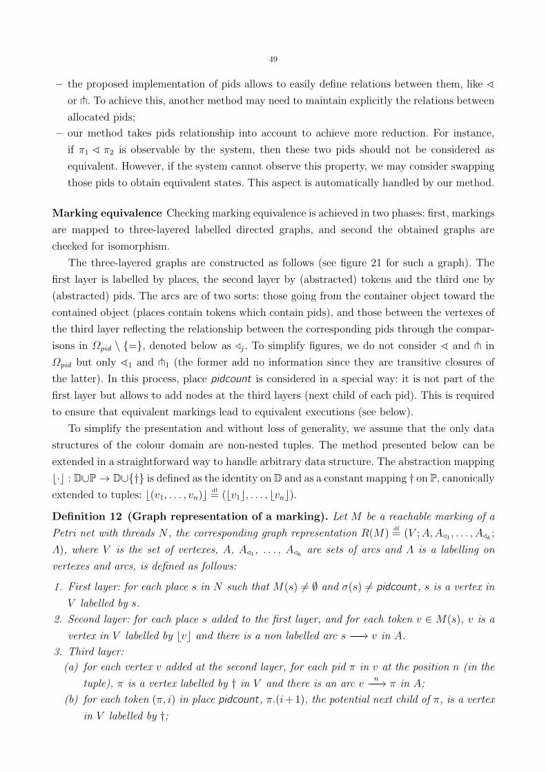
49

– the proposed implementation of pids allows to easily define relations between them, like ^or t. To achieve this, another method may need to maintain explicitly the relations between

allocated pids;

– our method takes pids relationship into account to achieve more reduction. For instance,

if π1 ^ π2 is observable by the system, then these two pids should not be considered as

equivalent. However, if the system cannot observe this property, we may consider swapping

those pids to obtain equivalent states. This aspect is automatically handled by our method.

Marking equivalence Checking marking equivalence is achieved in two phases: first, markings

are mapped to three-layered labelled directed graphs, and second the obtained graphs are

checked for isomorphism.

The three-layered graphs are constructed as follows (see figure 21 for such a graph). The

first layer is labelled by places, the second layer by (abstracted) tokens and the third one by

(abstracted) pids. The arcs are of two sorts: those going from the container object toward the

contained object (places contain tokens which contain pids), and those between the vertexes of

the third layer reflecting the relationship between the corresponding pids through the compar-

isons in Ωpid \ =, denoted below as /j. To simplify figures, we do not consider ^ and t in

Ωpid but only ^1 and t1 (the former add no information since they are transitive closures of

the latter). In this process, place pidcount is considered in a special way: it is not part of the

first layer but allows to add nodes at the third layers (next child of each pid). This is required

to ensure that equivalent markings lead to equivalent executions (see below).

To simplify the presentation and without loss of generality, we assume that the only data

structures of the colour domain are non-nested tuples. The method presented below can be

extended in a straightforward way to handle arbitrary data structure. The abstraction mapping

b·c : D∪P→ D∪† is defined as the identity on D and as a constant mapping † on P, canonically

extended to tuples: b(v1, . . . , vn)c df= (bv1c, . . . , bvnc).

Definition 12 (Graph representation of a marking). Let M be a reachable marking of a

Petri net with threads N , the corresponding graph representation R(M)df= (V ;A,A/1 , . . . , A/k ;

Λ), where V is the set of vertexes, A, A/1, . . . , A/k are sets of arcs and Λ is a labelling on

vertexes and arcs, is defined as follows:

1. First layer: for each place s in N such that M(s) 6= ∅ and σ(s) 6= pidcount, s is a vertex in

V labelled by s.

2. Second layer: for each place s added to the first layer, and for each token v ∈ M(s), v is a

vertex in V labelled by bvc and there is a non labelled arc s −−−−−−−−→ v in A.

3. Third layer:

(a) for each vertex v added at the second layer, for each pid π in v at the position n (in the

tuple), π is a vertex labelled by † in V and there is an arc vn−−−−−−−−→ π in A;

(b) for each token (π, i) in place pidcount, π.(i+ 1), the potential next child of π, is a vertex

in V labelled by †;

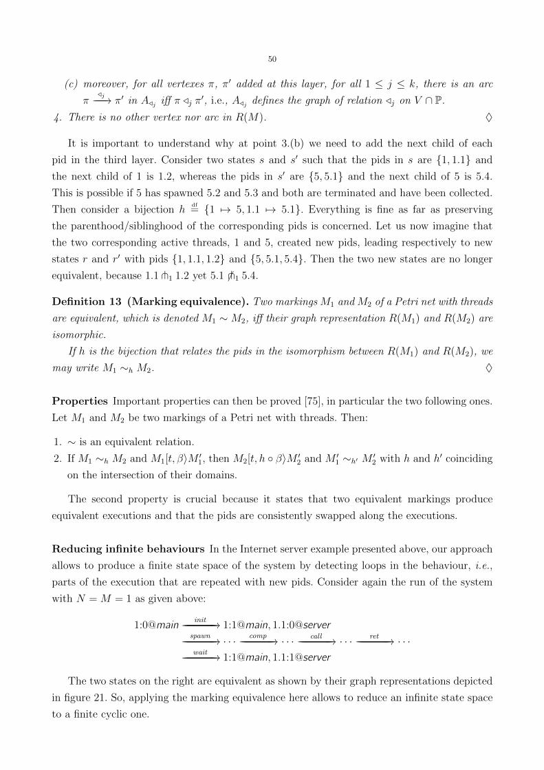
50

(c) moreover, for all vertexes π, π′ added at this layer, for all 1 ≤ j ≤ k, there is an arc

π/j−−−−−−−−→ π′ in A/j iff π /j π

′, i.e., A/j defines the graph of relation /j on V ∩ P.

4. There is no other vertex nor arc in R(M). ♦

It is important to understand why at point 3.(b) we need to add the next child of each

pid in the third layer. Consider two states s and s′ such that the pids in s are 1, 1.1 and

the next child of 1 is 1.2, whereas the pids in s′ are 5, 5.1 and the next child of 5 is 5.4.

This is possible if 5 has spawned 5.2 and 5.3 and both are terminated and have been collected.

Then consider a bijection hdf= 1 7→ 5, 1.1 7→ 5.1. Everything is fine as far as preserving

the parenthood/siblinghood of the corresponding pids is concerned. Let us now imagine that

the two corresponding active threads, 1 and 5, created new pids, leading respectively to new

states r and r′ with pids 1, 1.1, 1.2 and 5, 5.1, 5.4. Then the two new states are no longer

equivalent, because 1.1 t1 1.2 yet 5.1 6t1 5.4.

Definition 13 (Marking equivalence). Two markings M1 and M2 of a Petri net with threads

are equivalent, which is denoted M1 ∼M2, iff their graph representation R(M1) and R(M2) are

isomorphic.

If h is the bijection that relates the pids in the isomorphism between R(M1) and R(M2), we

may write M1 ∼h M2. ♦

Properties Important properties can then be proved [75], in particular the two following ones.

Let M1 and M2 be two markings of a Petri net with threads. Then:

1. ∼ is an equivalent relation.

2. If M1 ∼h M2 and M1[t, β〉M ′1, then M2[t, h β〉M ′

2 and M ′1 ∼h′ M ′

2 with h and h′ coinciding

on the intersection of their domains.

The second property is crucial because it states that two equivalent markings produce

equivalent executions and that the pids are consistently swapped along the executions.

Reducing infinite behaviours In the Internet server example presented above, our approach

allows to produce a finite state space of the system by detecting loops in the behaviour, i.e.,

parts of the execution that are repeated with new pids. Consider again the run of the system

with N = M = 1 as given above:

1:0@maininit−−−−−−−−−−−−−−−−−−−−−−−−−→ 1:1@main, 1.1:0@server

spawn−−−−−−−−−−−−−−−−−−−−−−−−−→ · · · comp−−−−−−−−−−−−−−−−−−−−−−−−−→ · · · call−−−−−−−−−−−−−−−−−−−−−−−−−→ · · · ret−−−−−−−−−−−−−−−−−−−−−−−−−→ · · ·wait−−−−−−−−−−−−−−−−−−−−−−−−−→ 1:1@main, 1.1:1@server

The two states on the right are equivalent as shown by their graph representations depicted

in figure 21. So, applying the marking equivalence here allows to reduce an infinite state space

to a finite cyclic one.

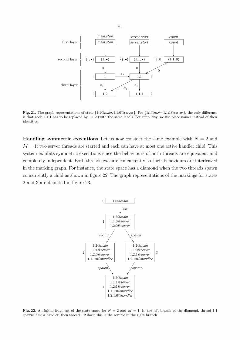
51

main.stop

main.stop

(1, •)(†, •)

1†

1.2†

server .start

server .start

(1.1, •)(†, •)

1.1 †

1.1.1 †

count

count

(1.1, 0)(†, 0)

0

^1

0

^1

^1

t1

0

first layer

second layer

third layer

Fig. 21. The graph representations of state 1:1@main, 1.1:0@server. For 1:1@main, 1.1:1@server, the only differenceis that node 1.1.1 has to be replaced by 1.1.2 (with the same label). For simplicity, we use place names instead of theiridentities.

Handling symmetric executions Let us now consider the same example with N = 2 and

M = 1: two server threads are started and each can have at most one active handler child. This

system exhibits symmetric executions since the behaviours of both threads are equivalent and

completely independent. Both threads execute concurrently so their behaviours are interleaved

in the marking graph. For instance, the state space has a diamond when the two threads spawn

concurrently a child as shown in figure 22. The graph representations of the markings for states

2 and 3 are depicted in figure 23.

1:0@main0

1:2@main

1.1:0@server

1.2:0@server1

1:2@main

1.1:1@server

1.2:0@server

1.1.1:0@handler

2

1:2@main

1.1:0@server

1.2:1@server

1.2.1:0@handler

3

1:2@main

1.1:1@server

1.2:1@server

1.1.1:0@handler

1.2.1:0@handler

4

init

spawn spawn

spawn spawn

Fig. 22. An initial fragment of the state space for N = 2 and M = 1. In the left branch of the diamond, thread 1.1spawns first a handler, then thread 1.2 does; this is the reverse in the right branch.

52

Because relation t1 has been taken into account (see the dotted edges in the graph represen-

tations), the two markings are not equivalent. However, it should be considered that nowhere

in the system t1 is used. So, the fact that two states are siblings or not cannot have any in-

fluence on the behaviour of the system. As a consequence, we can remove t1 from Ωpid . Doing

so, the graph representation of both states 1 and 2 becomes that depicted at the bottom of

figure 23 and the two graphs are now isomorphic. Indeed: let us first notice that the bottom

graph perfectly overlaps the middle graph; then, let us imagine that we flip the bottom graph

horizontally except its top row, then it would now perfectly overlap the top graph.

As a consequence, symmetric executions can now be identified, which results in a reduced

graphs where, in particular, only one interleaving of concurrent executions is considered.

Efficiency of graph isomorphism The complexity of checking graph isomorphism is, in

general, not known. In order to evaluate how efficient in practice it turns out to be in our

case, we generated random states and measured the time spent in checking isomorphism of the

corresponding graphs. We only considered pairs of markings where the same places are non-

empty. Indeed, pairs that do not match this way can be checked for non-equivalence in linear

time with respect to the number of places, without even converting them to graphs.

Our methodology has been to generate random states and compare each with similar ones

obtained through all possible transformations based on:

– pids swapping preserving isomorphism;

– shuffling of tokens throughout places;

– shuffling of tokens components (remember that tokens are tuples here);

– exchange of components between tuples (pids, data or both);

– data replacement;

– pids replacement;

– shifting of integers that compose pids.

To check graph isomorphism, we used NetworkX [60] that implements the VF2 [37] algorithm

that is considered as one of the fastest algorithms for graph isomorphism. We carried out more

than two millions of comparisons, on the basis of which it may be observed that:

– computation time is growing with the size of the markings and with the percentage of pids

in tokens (with respect to data);

– computation time improves when more distinct data values are involved in markings.

None of these observations should really be surprising. In particular, the presence of data leads

to labelled nodes that can be quickly matched when comparing two graphs.

Moreover, we observed that the general evolution of computation time is linear with respect

to p3/2 where p is the number of distinct pids in the compared states. With respect to p2, the

evolution of time is clearly sublinear. Hence it is justifiable to estimate that computation time

53

main.stop

main.stop

(1, •)(†, •)

1†

1.3†

server .start

server .start

(1.1, •)(†, •)

1.1†

1.1.1†

1.1.2†1.1.1.1†

(1.1, •)(†, •)

1.2 †

1.2.1 †

count

count

(1.1, 1)(†, 1) (1.2, 0)(†, 0)

0

^1

^1

0

^1

0

^1

^1^1^1t1t1

0 0

t1

main.stop

main.stop

(1, •)(†, •)

1†

1.3†

server .start

server .start

(1.1, •)(†, •)

1.1†

1.1.1†

(1.1, •)(†, •)

1.2†

1.2.2 †

1.2.1 †

1.2.1.1 †

count

count

(1.1, 0)(†, 0) (1.2, 1)(†, 1)

0

^1

^1

0 0

^1^1

^1 ^1 ^1t1 t1

0 0

t1

main.stop

(†, •)

†

†

server .start

(†, •)

†

(†, •)

†

† †

†

†

count

(†, 0) (†, 1)

0

^1

^1

0 0

^1^1

^1 ^1 ^1

0 0

Fig. 23. Top: the graph representation of state 2 from figure 22. Middle: the graph representation of state 3. Bottom:the graph representation of both states when t1 /∈ Ωpid , where nodes identities have been replaced by nodes labels.

54

is in mean polynomial (around p3/2) with respect to the number of threads in the observed

system. Finally, we determined that the computation time looks slightly less than quadratic

with respect to the number of tokens in compared markings.

It is worth noting that we observed similar results when, instead of considering random

states, we used states from the Internet server example presented above.

As a result, we conclude that the cost of checking state equivalence is very low for states

that are clearly different (most of the compared pairs) and stays good for states that are similar.

Moreover, it should be noted that discovering equivalent states allows to limit the state space

exploration. Thus the time spent in computing equivalences is likely to be often lower than the

time required to computed the whole state space, which obviously holds for infinite state spaces

reduced to finite ones. This reduction may also allow to analyze systems whose complete state

space would simply not fit into the computer’s memory, and thus would have been intractable

regardless of the computation time.

4.5 Related works

Petri nets with threads have been initially defined with a syntax that extends the pbc syntax

with task construction and trap operator [112], as well as with time-related operations inspired

from [110] (see also section 5.1).

A modelling of multi-tasking systems in the context of M-nets has been proposed in [80],

based on a Petri net model developed in [78, 79]. However, it relied on general preemption

operators allowing to suspend, resume or abort arbitrary M-nets, including with nested parallel

compositions. To achieve this level of generality, the coloured Petri net model has been extended

with priorities between transitions. The setting proposed above is much simpler and, at the

same time, it is just as expressive. Indeed, every task can be constructed in a way that allows

to suspend, resume or abort the corresponding threads, as depicted in figure 24. The idea is to

add three places for a task named task :

– when a thread is started as an instance of task , its pid is added to place task .run;

– every transition in the task is added a side loop or a read arc labelled by π to this place

so it can progress only if its pid is present here (a side loop does not reduce concurrency

because a thread is already sequential);

– place task .suspend is the complementary place of task .run; so, to suspend a thread, its pid

has to be moved from place task .run to task .suspend ;

– to resume the execution of a suspended thread, its pid has to be moved back from place

task .suspend to task .run;

– finally, to abort a thread, its pid is removed from task .run and added to task .suspend and

task .abort. This enables transition ta that directly terminates the thread by putting the

appropriate token in the stop place of the task;

55

– to be correct, the input control flow places of ta must be exactly the same as for t, but the

arcs to ta must be labelled with (π, x) so the thread may be aborted in both regular and

exception control flow.

t...

t...

ta

(π, x)

Ptask .abort

Ptask .suspend

Ptask .run

π

π

π

P× •, task .stop

(π, )

Fig. 24. Left: a transition in its context within a task; the depicted places are control flow places. Right: the sametransition with additional context to support preemption.

The transformation proposed above to enable for external preemption leads to increase the

size of Petri nets. In particular, the number of transitions is multiplied by two whereas three

places per task are added. However, it should be noted that this is comparable with the solution

adopted for preemptible M-nets from [78–80]. Moreover, transitions priorities used in this model

can be removed by transforming the nets, but to the price of a huge blow-up which is far more

than doubling the number of transitions and leads to intractable nets. On the other hand, using

priorities makes it possible to implement efficient garbage collection: tokens corresponding to

terminated threads, in particular tokens in data places, can be removed from the Petri net

using prioritised transitions, which can be achieved before any other transition in the net is

allowed to fire. In the context of Petri nets with threads, collecting garbage tokens cannot be

prioritised and thus we cannot guarantee that a token from a terminated thread if ever removed

from the corresponding task. However, because pids are never reused, these tokens cannot be

confused with tokens owned by another thread executed later on. They can be considered as

garbage, which may be collected in the background if one wants to model a garbage collector;

they could be ignored by the model-checker to reduce combinatorial explosion; or it may even

be the purpose of such an analysis to decide whether garbage tokens exist or not.

The marking equivalence technique presented to reduce state spaces of Petri nets with

threads is actually an instance of a more general equivalence reduction method defined for

coloured Petri nets in [69]. This method requires an equivalence specification to be consistent [69,

def. 1], i.e., preserved along the executions of a system, which in our case is a corollary of

the properties of ∼h. As noted in [67, sec. 8.4], proving the consistency is often a complex

prerequisite to use equivalence reduction. And indeed, establishing the properties of ∼h required

quite an involved proof [75]. But this has been done in a general setting and can then be reused

in many contexts with a reasonable effort.

56

Verification of multi-threaded systems is a very active topic, possibly because threading is

the major paradigm of concurrency in nowadays programming languages. A variety of methods

such as those in [33, 66, 68] (see, e.g., [92] for a survey) address the state explosion problem by

exploiting, in particular, symmetries in the system in order to avoid searching parts of the state

space which are equivalent to those that have already been explored. Some methods, such as [18,

63, 86], have been implemented in widely used verification tools and proved to be successful

in the analysis of numerous communication protocols and distributed systems. The method

proposed in this paper actually focuses on abstracting thread identifiers and symmetries are

addressed only indirectly. So, not only it reduces symmetric executions but also it can cope with

infinite repetitive behaviours. Moreover, it should be noted that symmetry reduction techniques

rely on the computation of a canonical representation of each state. It has been shown in [36]

that this is as hard as computing a graph isomorphism. So, our method, while being more

general than symmetry reduction, is not computationally more complex.

Our approach appears to be closely related to that developed in [68] (which, incidentally,

covers those in [66, 33]) where a general framework was proposed aiming at reduced state space

exploration through the utilisation of symmetries in data types. More precisely, [68] defines

three classes of primitive data types. Two of these, ordered (for which symmetries are not

considered) and cyclic (which are finite) cannot lead to reductions based on pids. The remaining

one, unordered, can in principle be used for reduction even for an infinite domain [68, section

7.5]. However, the approach proposed in [68] does not cover the case of dynamic process creation

as considered here. Moreover, when comparing two states for equivalence, the approach of [68]

considers only data actually present in the states. In our case, however, we have to look at

additional data (potential children of the pids present in the states) to ensure the preservation

of equivalence over possible behaviours. We believe that approaches like [68] can be combined

with ours to the price of explicitly maintaining in the model the information about relationships

between active pids such as the siblinghood, as well as about their next pids.

5 Applications

5.1 Modelling time by causality

Starting from [109], we have introduced the modelling of time through explicit representation

of clocks in a model. Basically, a clock is composed of a tick transition that increments or

decrements counters stored in places typed by Nωdf= N ∪ ω, where ω is an integer-like value

such that ω + idf= ω and ω > i for all i ∈ Z. Incrementing counters allows to measure the

passing of time, decrementing counters allows to specify structural timing constraints that the

system cannot overcome. This is illustrated in figure 25:

– at the initial state, ticks can occur without changing the marking;

– when t1 fires, it replaces the counters so that min = 0 and max = 10;

– because of its guard, t2 is now disabled until min reaches at least 3;

57

– each tick occurrence increments the value of min and decrement the value of max . The

former can be incremented infinitely but the latter cannot decrease below zero;

– so t2 becomes enabled after three tick occurrences, but no more than ten ticks can occur

because of the minimal value allowed for max ;

– when t2 fires, it replaces counter max with ω so that ticks can occur again if max had already

reached zero.

Assigning a non-ω value to a decreasing counter can be considered as setting a structural dead-

line; conversely, assigning ω to such a counter can be seen as releasing the deadline constraint

because this counter cannot block anymore the occurrence of ticks.

• t1

ωmin

Nω

√

ωmax

Nω

t2x ≥ 3

x 7→ 0

y 7→ 10

x

y 7→ ω

x 7→ x+ 1

y 7→ y − 1

Fig. 25. A simple causally timed system with two counters min and max and a tick transition√

. Transition t2 must firewhen at least 3 and at most 10 ticks have occurred since t1 has fired.

Such a system models time but actually only involves causality relations between transitions.

That is why we say that time is modelled by causality. Several interesting characteristics of this

approach have been shown, in particular:

– it is usable for practical system modelling and verification, it can even be more efficient than

timed-automata based approaches [26];

– several ticks may be used, they can be kept independent or synchronised [109];

– timing features can be introduced in syntactic layers, avoiding to the user the task to deal

with clock modelling [110, 112];

– under reasonable assumption, a causally timed Petri net can be executed in a real time

environment in such a way that ticks occur evenly with respect to environment’s time (this

is detailed below);

– the extra state explosion introduced by tick counters can be compensated for by using

appropriate abstraction, even allowing in some cases to compute infinite state spaces (see

below).

Real-time execution When considering a causally timed system, the question arises whether

this system is realistic or not: if we consider an external observer, equipped with a watch, who

58

looks at tick occurrences, can we arrange any execution of the system so that ticks occur evenly

from the observer’s point of view?

It turns out that this is not possible in general. For instance, consider the system depicted

in figure 25. If we add a transition t3 connected to the bottom place with a side loop, then,

the number of firings of t3 between t1 and t2 is unbounded. But we cannot in a finite amount

of observer’s time execute arbitrarily many firings of t3, except if firing transitions takes no

computation time which is not realistic at all. The problem with t3 is that it can be repeated

arbitrarily with no requirement that time progresses. This is sometimes called a Zeno execution.

In [111, 113], we define a notion of tractable Petri nets with causal time. Such a Petri net

is tractable if there exists a constant δ such that any sequence of at least δ transition firings

contains at least two ticks. This is to say that only bounded execution can occur between

two ticks. So, by choosing a large enough duration in observer’s time, any execution can be

scheduled in such a way that ticks occurrences are even from the observer’s point of view.

Moreover, since we are considering an observer, we can address the question of communica-

tion between the Petri net and its observer. It is easy to produce output to the environment: the

observer simply looks at more than just the tick transition. But it is more complicated to take

into account at the Petri net side inputs from the environment. Indeed, the observer should not

be allowed to modify the Petri net states nor to force events to occur (this would violate the

semantics) but may just ask for some specific events to take place, if they are possible. This

can be formalised as a notion of input ports, each consisting of a transition t and a subset of

variables from vars(t). An input from the environment to the Petri nets becomes a request that

a specific transition is executed with a chosen binding of the selected variables. Then, we can

define a notion reactive transitions to ensure that such a request is always handled within at

most one tick. Reactive transitions are easy to implement using side loops while keeping the

Petri net tractable; an example is shown in figure 26.

12

3N t

x > 0

ω

Nω

delay√y x 7→ 0 x 7→ ω

Fig. 26. A Petri net with causal time where transition t is reactive with respect to input port (t, y). The connectionof t with the clock ensures that the net is tractable because t cannot fire more than once between two ticks.

Verification issues Causal time approach is convenient because it allows to verify systems

including timing aspects using any tool that supports coloured Petri nets. However, explicitly

counting ticks increases the state explosion problem. Consider for example the Petri net given

in figure 25, it has three “logical” states: (1) before t1, (2) between t1 and t2, and (3) after

t2. However, when considering its concrete states, we have to take into account all the possible

values of the counters. For instance, in (2) we may have any valuation (min,max) ∈ (i, 10− i) |

59

0 ≤ i ≤ 10; i.e., 11 different states. Worst, in (3) we have (min,max) ∈ (i, ω) | i ≥ 3; i.e.,

infinitely many equivalent states.

The second problem, i.e., counting up to ω, can be fixed by replacing ω with the largest

constant to which a counter is compared to, plus 1. For instance, in the system of figure 25, we

can set ωdf= 4. Then, expression like x + 1 that label output arcs from the tick transition can

be replaced with expressions like min(ω, x+ 1). This way, the behaviour of the system remains

essentially the same but its state space is finite.

The first problem remains: tick counters introduce many equivalent markings in the state

space. The problem is worst when several independent counters are used. In the previous ex-

ample, min and max are not independent since we have max = 10−min in (2). In this case, the

possible values of these counters do not combine in a way that increases the state space size. But

consider two identical systems, just sharing the same tick transition, and distinguish them by

putting primes in the second copy. There exists a kind of synchronisation through time between

these two systems; but, since the firing of t1 and t′1 are not related, the whole Petri net may

reach 9 logical states as shown in figure 27. Considering that we have set ωdf= 4 as explained

before, (3) and (3′) correspond to 2 concrete states (min ∈ 3, 4). Then, the total number of

concrete state is 196. In general, we can observe that independent timed subsystems contribute

in a multiplicative way to the number of states, which leads to an exponential combinatorial

explosion.

(1, 1′)

(1, 2′)

(1, 3′)

(2, 1′)

(2, 2′)

(2, 3′)

(3, 1′)

(3, 2′)

(3, 3′)

⇒ (1× 1) = 1

⇒ (1× 11) + (11× 1) = 22

⇒ (1× 2) + (11× 11) + (2× 1) = 125

⇒ (11× 2) + (2× 11) = 44

⇒ (2× 2) = 4

Fig. 27. The logical states corresponding to the interleaving of (1)t1−−−−−−−−−→ (2)

t2−−−−−−−−−→ (3) and (1′)t′1−−−−−−−−−→ (2′)

t′2−−−−−−−−−→ (3′). On theright is indicated the number of concrete states in each row of logical states.

This problem is addressed in [117] by proposing a model of Petri nets equipped with counters

that are no more modelled has places. Instead, their values are stored in vectors of integers kept

aside each marking: a state becomes a pair (M, v) where M is a marking and v is a vector that

provides the valuation of counters. Each transition t is allowed to test a condition Ct on the

counters and to update them using a transformation Ut. Then, we use a library [17] to represent

efficiently large or infinite sets of such vectors, and to perform computation on these sets, like

shifting by ±1 all the components of all the vectors in a set. More interesting, it is possible to

compute the accumulated effect of arbitrarily many repetitions of such a shifting. This allows

60

to define an abstract state space construction in which an abstract state is a pair (M,V ) where

M is a marking and V is a set of vectors. When a transition fires, we have (M,V )[t〉(M ′, V ′)

with M ′ computed from M as usual and V ′df= Ut(v) | Ct(v)∧ (v ∈ V ). If V ′ = ∅ then t is not

enabled (no concrete state passes condition Ct).

The idea to achieve compression is based on the detection of cycles in the state space with

respect to the marking. Let (M ′, V ′) be a newly computed abstract state, several situations are

possible:

– no abstract state of the form (M ′, V ′′) has been reached before, then we can add (M ′, V ′)

to the abstract state space;

– there exists already an abstract state (M ′, V ′′) such that V ′′ ⊇ V ′, then we have reached

already known states;

– there exists already an abstract state (M ′, V ′′) such that V ′′ ⊂ V ′, then we have found a

cycle in the behaviour that loops through M ′ while reaching new valuation of counters. So,

it is likely that from (M ′, V ′′) we can repeat again and again the same sequence t1, . . . , tk

of transitions. This sequence corresponds to a transformation Ut1,...,tk that can be computed

and we can also compute the repeated effect of Ut1,...,tk on V ′′, denoted by U∗t1,...,tk(V′′). This

corresponds to simulate in a finite computation the (possibly) infinite repetition of the same

sequence of transitions. So, (M ′, V ′′) is replaced by (M ′, U∗t1,...,tk(V′′)) in the state space (and

its future is recomputed);

– finally if we observe a firing (M ′, V )[t〉(M ′, V ′), we can expect t to be repeatable at M ′. So

we store (M ′, U∗t (V )) instead of (M ′, V ) in the state space (and its future is recomputed).

This allows to compress sequences of transitions that update counters but do not change

the marking, which is typically the behaviour of a tick transition (but not only).

In general, this method cannot be guaranteed to terminate when the concrete state space is

infinite. But, on practical examples, it allows for efficient computation of large and even infinite

state spaces. Typically, infinity that comes from the repeated incrementation of some counters is

successfully tackled by the method. Moreover, we can show a behavioural equivalence between

a Petri net equipped with external counters and its translation into a coloured Petri net in

which counters are explicitly implemented as integer-valued places. More precisely, if N is a

Petri net with counters and N ′ is its coloured implementation, we can show that:

– the set of reachable states of N and N ′ are essentially the same (we just have to translate

between vector-based and place-based implementation of counters);

– any trace of N ′ is a path in the abstract state graph of N ;

– for any path in the abstract state graph of N , it can be checked whether it is a trace of N ′

or not by using only N .

The first point shows that the approach is exact with respect to reachability: no information

is loosed not added. The second and third points show that the abstract state space is an

61

over-approximation of the concrete state space in that it includes paths that are not realisable

sequences of transitions. However, checking the realisability of such a path does not require

to compute the concrete state spaces nor the coloured implementation of the Petri net with

counters.

Related works The causal time calculus as been proposed in [110] has an extension of the

pbc to provide a syntax for causally timed systems, together with an operational semantics.

Extended syntactical features have been later proposed in the context of multi-threaded sys-

tems [112]. Other timed extensions of the pbc have been proposed, however they are not based

on the causal time approach but rather on various extensions of Petri nets with time; in par-

ticular, [82] and [2] introduce the features of time Petri nets [89] and timed Petri nets [122]

respectively.

The question of efficiently verifying counter systems is addressed by numerous tools among

which: fast [7], mona [50], Omega [119] and sataf/PresTaf [38]. In [117], we used Lash li-

brary [17] to carry out experiments. These tools use various techniques and theories to efficiently

deal with counter systems. However, it is likely that our approach may be adapted to use any

of these tools since it treats in a separate way the aspects related to Petri nets on the one hand,

and counters on the other hand, the latter being fully delegated to the library. A more dras-

tic approach is proposed in [8] where Petri nets are completely translated to counter machines

which are then verified with fast. This is possible since p/t nets are considered so the marking

of each place can be encoded as a counter; however, this would not apply to our model that is

based on coloured Petri net.

5.2 Specification and verification of security protocols

In this section, we show how the abcd language introduced in section 3.3 can be used to specify

and verify security protocols. As an illustration, we model Needham&Schroeder’s protocol for

mutual authentication [99]. This is quite a small example, but abcd is also used in the context

of project spreads that aims at building a secure platform for distributed network storage

with peer-to-peer architecture (see [133] for more information). These protocols are still under

development and are anyway too big to be shown here. Fortunately, Needham&Schroeder’s

protocol allows to show the most important aspects about applying abcd to security protocols.

Needham&Schroeder’s protocol for mutual authentication The protocol ns involves

two agents Alice (A) and Bob (B) who want to mutually authenticate. This is performed through

the exchange of three messages as illustrated in figure 28. In this specification, a message m

is denoted by 〈m〉 and a message encrypted by a key k is denoted by 〈m〉k (we use the same

notation for secret key and public key encryption). The three steps of the protocol can be

understood as follows:

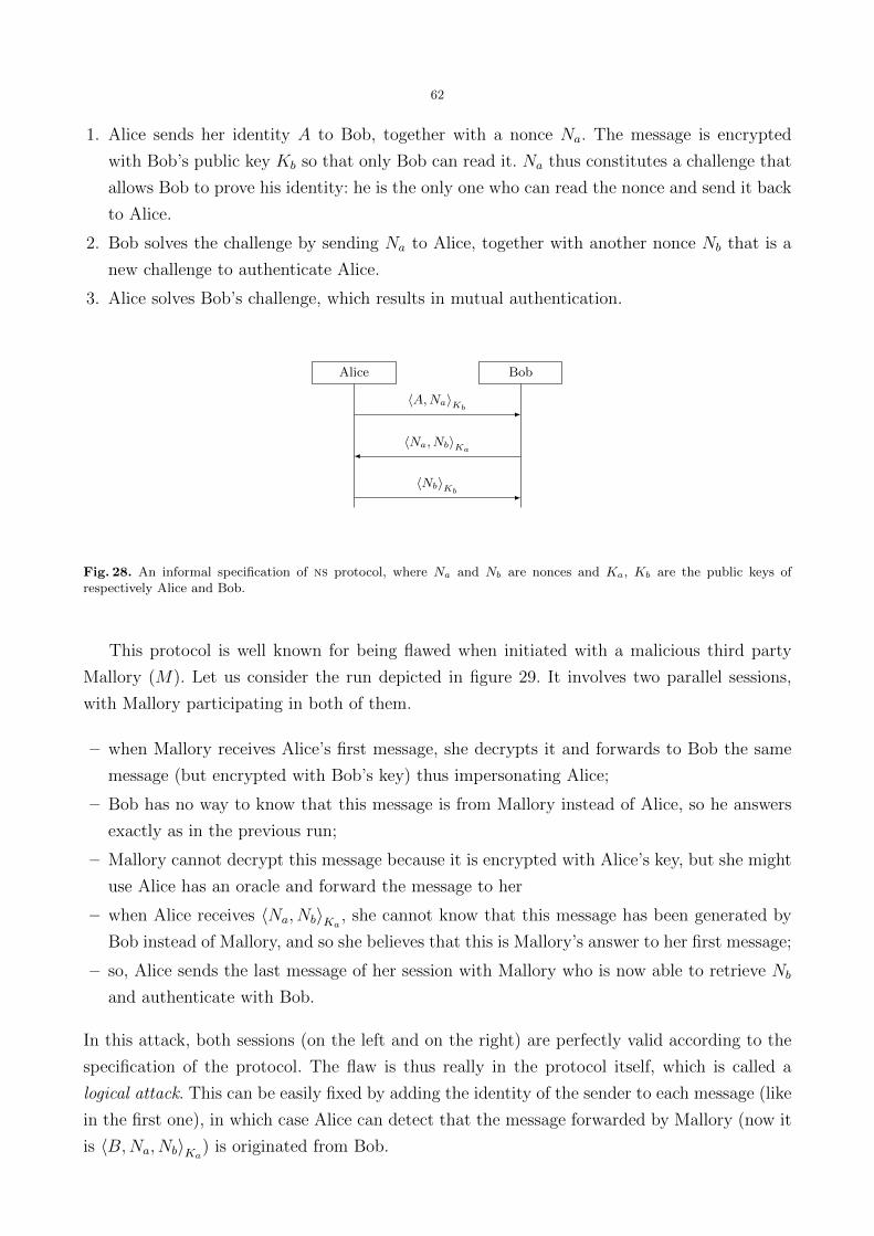
62

1. Alice sends her identity A to Bob, together with a nonce Na. The message is encrypted

with Bob’s public key Kb so that only Bob can read it. Na thus constitutes a challenge that

allows Bob to prove his identity: he is the only one who can read the nonce and send it back

to Alice.

2. Bob solves the challenge by sending Na to Alice, together with another nonce Nb that is a

new challenge to authenticate Alice.

3. Alice solves Bob’s challenge, which results in mutual authentication.

Alice Bob

〈A,Na〉Kb

〈Na, Nb〉Ka

〈Nb〉Kb

Fig. 28. An informal specification of ns protocol, where Na and Nb are nonces and Ka, Kb are the public keys ofrespectively Alice and Bob.

This protocol is well known for being flawed when initiated with a malicious third party

Mallory (M). Let us consider the run depicted in figure 29. It involves two parallel sessions,

with Mallory participating in both of them.

– when Mallory receives Alice’s first message, she decrypts it and forwards to Bob the same

message (but encrypted with Bob’s key) thus impersonating Alice;

– Bob has no way to know that this message is from Mallory instead of Alice, so he answers

exactly as in the previous run;

– Mallory cannot decrypt this message because it is encrypted with Alice’s key, but she might

use Alice has an oracle and forward the message to her

– when Alice receives 〈Na, Nb〉Ka , she cannot know that this message has been generated by

Bob instead of Mallory, and so she believes that this is Mallory’s answer to her first message;

– so, Alice sends the last message of her session with Mallory who is now able to retrieve Nb

and authenticate with Bob.

In this attack, both sessions (on the left and on the right) are perfectly valid according to the

specification of the protocol. The flaw is thus really in the protocol itself, which is called a

logical attack. This can be easily fixed by adding the identity of the sender to each message (like

in the first one), in which case Alice can detect that the message forwarded by Mallory (now it

is 〈B,Na, Nb〉Ka) is originated from Bob.

63

Alice Mallory Bob

〈A,Na〉Km

〈A,Na〉Kb

〈Na, Nb〉Ka

〈Na, Nb〉Ka

〈Nb〉Km

〈Nb〉Kb

Fig. 29. An attack on ns protocol where Mallory authenticates as Alice with Bob.

Modelling communication and cryptography Using abcd, a simple model of a network

is a globally shared buffer: to send a message we put its value on the buffer and to receive a

message, we get it from the buffer.

Messages can be modelled by tuples and cryptography can be treated symbolically, i.e., by

writing terms instead of by performing the actual computation. For instance, the first message

in ns protocol may be written as a nest of tuples ("crypt", ("pub", B), A, Na):

– string "crypt" denotes that the message is a cryptogram, the encryption key is thus expected

as the second component of the tuple and the following components form the payload;

– tuple ("pub", B) indicates that this is a public key owned by B (we will see later on how to

model agents’ identities);

– the payload is the message (A, Na) (we will see later on how to model nonces).

Using this modelling, messages actually travel in plain text over the network. But if we adopt

the Dolev&Yao model [48] and correctly implement it, this is a perfectly valid approach. In

Dolev&Yao’s model, the attacker is considered to reside on the network. So, Mallory can read,

remove or even replace any message on the network. Moreover, she can learn from the read mes-

sages by decomposing them and looking at their content. However, cryptography is considered

to be perfect and so, Mallory cannot decrypt a message if she does not know the key to do so.

For instance, if she reads ("crypt", ("pub", B), A, Na) on the network, she is allowed to learn

A and Na only if she already knows Bob’s private key ("priv", B). To correctly implement

Dolev&Yao’s model, we shall ensure that no agent can perform any action on an encrypted

content knowing the key to do so.

Then we need to model agents’ identities. In this protocol, we can just use positive integers

because no such value is used somewhere else so there is no risk of confusion with another

message fragment.

64

To model nonces, we cannot rely on a random generator unlike in implementations: this

would lead to undesired non-determinism and possibly to a quick combinatorial explosion. To

correctly model perfect cryptography while limiting state explosion, we must find an encoding

such that:

– each nonce is unique;

– a nonce cannot be confused with another value;

– nonces can be generated in a deterministic way.

In our case, a simple solution is to program them a Python class Nonce. The constructor expects

an agent’s identity; for instance, Nonce(1) denotes the nonce for the agent whose identity is 1.

Equality of two nonces is then implemented as the equality of the agents who own these nonces.

To respect Dolev&Yao’s model, we must forbid an agent to generate a nonce using another

agent’s identity.

So, let us call nw (for “network”) the buffer that supports network communication and allow

it to store any token (type object); moreover, let us import the content of a module dolev yao

that defines class Nonce:

1| buffer nw : object = ()2| from dolev yao import ∗

Modelling Alice and Bob Each agent can be modelled as a sub-net. For instance, Alice can

be modelled as follows:

1| net Alice (this , agents) :2| buffer peer : int = ()3| buffer peer nonce : Nonce = ()4| [agents?(B), peer+(B), nw+("crypt", ("pub", B), this, Nonce(this))]5| ; [nw−("crypt", ("pub", this), Na, Nb), peer nonce+(Nb) if Na == Nonce(this)]6| ; [peer?(B), peer nonce?(Nb), nw+("crypt", ("pub", B), Nb)]

Parameter this provides the agent’s identity, which is concretely provided when the sub-

net is instantiated. This allows us to create several differentiated instances of Alice if needed.

Parameter agents is expected to be a global buffer containing the identities of all the agents

that Alice is allowed to contact. Line 5, a local buffer is declared to store the identity of the

peer initially contacted by Alice. Line 6, another local buffer is declared to store peer’s nonce

received by Alice in the second message, in order to be able to forward it in the third message.

Line 7, Alice gets one value from buffer agents (i.e., chooses one peer to contact) and puts it into

her buffer peer; she also sends the first message by producing the appropriate token in the global

buffer nw. Line 8, Alice receives a message by consuming a token on nw, the received message

is specified as a nest of tuples that forms a pattern to match the received message. Doing so,

variables Na and Nb are bound to actual values from the message. In the same action, it is

checked that Na has the correct value. Notice that this action respects Dolev&Yao’s model: the

content of the message is examined but the action is allowed to take place only if the received

65

message is encrypted with Alice’s key. Then, line 9, Alice sends the last message as expected

by Bob whose nonce is fetched from the local buffer peer nonce (without consuming it since

the interrogation mark denotes a read arc). Lines 7–9 define one atomic action each and these

three actions are composed sequentially.

The model for Bob is similar with two main differences: messages are specified from the

receiver’s point of view, and peer’s identity is discovered from the first message instead of being

chosen from a buffer. Apart from these changes, the specification is really similar:

1| net Bob (this) :2| buffer peer : int = ()3| buffer peer nonce : Nonce = ()4| [nw−("crypt", ("pub", this), A, Na), peer+(A), peer nonce+(Na)]5| ; [peer?(A), peer nonce?(Na), nw+("crypt", ("pub", A), Na, Nonce(this))]6| ; [nw−("crypt", ("pub", this), Nb) if Nb == Nonce(this)]

Modelling Mallory To model Mallory, we need to implement Dolev&Yao’s attacker. She

maintains a knowledge base k containing all the information learnt so far and repeatedly exe-

cutes the following algorithm:

1. Get one message m from the network.

2. Learn from m by decomposition or decryption using a key already in k. Whenever a new

piece of information is discovered, add it to k and recursively learn from it.

3. Optionally, compose a message from the information available in k and send it on the

network.

The last action is optional, which means that a message may be removed from the network with

nothing to replace it. This corresponds to a message destruction, which the attacker is allowed

to do. Notice also that, when composing a new message, Mallory may rebuild the message she

has just stolen. This corresponds to a message eavesdropping, which the attacker is also allowed

to do.

The hard part in modelling this attacker is the message decomposition and composition

machinery. This is feasible with just Petri nets (and has been done in [20]) but is really com-

plicated and leads to many intermediate states that quickly make the state space intractable.

Fortunately, using abcd, we can implement this part in Python. So, module dolev yao also

provides a class Spy that implements Dolev&Yao’s attacker. Only the algorithmic part is imple-

mented, taking into account our conventions about symbolic cryptography. For instance, tuples

like ("crypt", · · ·) or ("pub", · · ·) are correctly recognised as special terms.

To reduce combinatorial explosion in the state spaces, an instance of Spy is given a signature

of the protocol. This consists in a series of nested tuples in which the elements are either values

or types. Each such tuple specifies a set of messages that the protocol can exhibit. For instance,

ns protocol has three types of message:

– ("crypt", ("pub", int), int, Nonce) corresponding to the first message;

66

– ("crypt", ("pub", int), Nonce, Nonce) corresponding to the second message;

– ("crypt", ("pub", int), Nonce) corresponding to the third message.

This information is exploited by the attacker to avoid composing pieces of information in a

way that does not match any possible message (or message part) in the attacked protocol.

Without this mechanism, learning just one message m would lead the attacker to build an

infinite knowledge containing, e.g., (m,m), (m,m,m), (m, (m,m)), etc. However, this would

be completely useless unless such values would be parts of the protocol and may be accepted

as a message by an agent if these values were sent on the network. So, the attacker uses the

protocol signature to restrict the knowledge to valid messages or message parts.

The knowledge part of the attacker is modelled by a Petri net place, i.e., by an abcd buffer.

This allows to observe in the state space what the attacker has learnt, for instance to check for

leaking secrets. This knowledge has to be initialised, in our case, we would like Mallory to be

able to initiate a communication with another agent. So we shall provide her with an identity,

and the corresponding nonce and private key. We shall also provide the list of other agents and

their public keys. So, Mallory is specified as follows:

1| net Mallory (this, init ) :2| buffer knowledge : object = (this, Nonce(this), ("priv", this)) + init3| buffer spy : object = Spy(("crypt", ("pub", int), int, Nonce),4| ("crypt", ("pub", int), Nonce, Nonce),5| ("crypt", ("pub", int), Nonce))6| ([spy?(s), nw−(m), knowledge>>(k), knowledge<<(s.learn(m, k))]7| ; ([True] + [spy?(s), knowledge?(x), nw+(x) if s.message(x)]))8| ∗ [False]

Parameter this is like for the other agents, parameter init is intended to be a tuple of initially

known pieces of information. Line 19, Mallory’s knowledge is declared and initialised: it contains

her identity, nonce and private key, plus all the information from init. Line 20, an instance of

Spy is created in a buffer spy, with the signature of the protocol. Then comes the infinite loop

(because of the impossible exit line 25) to execute the attacker’s algorithm:

– line 23, a message m is removed from the network with nw−(m), the content of buffer

knowledge is flushed to variable k with knowledge>>(k) and replaced with all that can be

learnt from m and k, thanks to knowledge<<(s.learn(m, k));

– line 24, either [True] is executed (do nothing), or a value x is fetched from knowledge and

put on the network, but only if it is a valid message, which is checked in the guard.

Notice that this model of attacker is generic (except possibly for its initial knowledge) and

one may safely copy/paste its code to another specification.

Defining and verifying a scenario To create a complete abcd specification, we need to

provide a main term. This consists in a composition of instances of the defined agents. By

providing this, we create a scenario, i.e., a particular situation that can then be analysed. Let

67

us consider a simple scenario with one instance of Alice, one of Bob and one of Mallory; a buffer

agents will store the identities of Bob and Mallory so that Alice will contact one or the other at

the beginning. This scenario includes the possibility for Mallory to try to authenticate with Bob

since we gave to her enough knowledge to play the protocol. So, this simple scenario involves

all kind of communications between honest and dishonest agents. Notice that including more

than one attacker would result in a quick state explosion; fortunately, this is rarely needed and

if so, may be simulated by providing more than one identity to the same and only attacker.

Our scenario is thus specified as:

1| buffer agents : int = 2, 32| Alice(1, agents) | Bob(2) | Mallory(3, (1, ("pub", 1), 2, ("pub", 2)))

Using the abcd compiler, we can create a pnml file from this system. This file can be loaded

from a Python program using snakes to build the state space and search for a faulty one where

Alice and Bob are in a final state (i.e., their exit places are marked) and mutual authentication

is violated (i.e., data in buffers peer and peer nonce of each agent are not consistent).

The state space has 2048 states among which one shows that Alice authenticated Bob

but Bob authenticated Mallory, which corresponds to the known attack. There are also states

showing that both Alice and Bob may authenticate Mallory, but these are just regular runs

of two parallel sessions (Alice with Mallory and Bob with Mallory). When looking closer to

the states, we can see that Mallory is able to use someone else’s nonce for authentication: for

instance she may use Alice’s nonce as a challenge for Alice. This is not an error in the protocol

and is fully consistent with the fact that nonces freshness is never tested.

Related works In order to specify security protocols, formal description languages have been

proposed, like the spi-calculus [1] or the security protocol language, spl [41]. The latter is an eco-

nomical process language inspired from process algebras like the asynchronous π-calculus [93]:

each process is defined by a term of a specialised algebra which allows to represent sequences

and parallel compositions of input and output actions that may handle messages. Thus, in

contrast to frequently used notations like the message sequence chart of figure 28 or textual

variants (so called “Alice/Bob notations”), sending and receiving messages have to be specified

separately.

Previous experiences with spl [22, 20] showed that it only has a limited expressivity that

restrict its possible usages: a protocol in spl can only be specified using parallel and sequential

compositions of send or receive actions, and no initial knowledge can be specified. Many useful

features are not provided by spl, in particular: looping or recursion, choice (with conditional

execution), explicit data storage and manipulation, local computation (i.e., actions with no

communication), and of course initial knowledge. This last point has motivated extensions of

spl in [21, 22, 20]. As shown above, this feature is provided by abcd as well as the other desired

features. This is particularly important in the context of project spreads [133]: parts of the

studied peer-to-peer protocols involve exchanging lists of peers identities, the length of which

68

being not known in advance, and then communicate with a chosen subset of peers from the

lists. Here, the capability of abcd to express data structures (e.g., lists) and complex control

flow (e.g., iterating over a list) is a crucial aspect.

One more aspect of spl is arguably a drawback or an advantage: when a message is received,

it can be matched against a pattern, doing so, the variables in the pattern are bound to the

received values and this is recorded for the whole future of the process (as usual in process

algebras). This feature is very convenient for the ease of specification, but on the other hand, it

hides important aspects of information management in the agents. In comparison, using abcd,

one has to explicitly specify data storage. This might be considered as tedious but it has at

least three advantages:

– the model is closer to an implementation in that not only it specifies how communication

takes place, but also it shows which piece of information should be stored by each agent;

– parts of this information may be security critical, for instance cryptographic keys. Explicitly

modelling their storage makes it possible to analyse these aspects, for instance information

leak;

– using an explicit modelling of the spy allows to use any general purpose model checker to

verify the modelled protocols, instead of being forced to use a model-checker that implements

the spy.

Looking at the spore or avispa protocols collections [132, 6] we can observe that most of the

analysed protocols listed on the page do not need loop or choice. This could be an argument

against our claim that such features are needed. However, other protocols involve complex

control flow and have been verified, but not using tools dedicated to protocols; see for instance

the industrial case studies from the web pages of cpn tools [40]. It is worth noting that we

advocate for tools with rich control flow and extensive data domain, not for abcd in particular.

Indeed, not every aspect of protocols verification can be addressed using a symbolic treatment

of cryptography. For example, approaches like [15, 16] can represent aspects of protocols like

algebraic properties of cryptographic primitives. For some protocols, like Diffie&Helman’s key

exchange [47], these are required features in order to correctly address the security concern. It

is likely that this case can be handled in abcd by implementing dedicated classes in Python,

like we did for the treatment of nonces. This shows that an expressive data model is very much

required and, thanks to a mixture of modelling and implementation, lacks in the analysis tool

may be compensated for by user-defined extensions of the data model.

5.3 Modelling biological regulatory networks

Great advances in molecular biology, genomics and functional genomics open the way to the

understanding of regulatory mechanisms controlling essential biological processes. These mech-

anisms interplay and operate at diverse levels (transcription and translation of the genetic

material, protein modifications, etc.). They define large and complex networks, which in turn

69

constitute a relevant functional integrative framework to study the regulation of cellular pro-

cesses. To assess the behaviours induced by such networks, dedicated mathematical and compu-

tational tools are very much required. In general, mathematical models for concrete regulatory

networks are defined as a unique whole, considering networks of a limited size (up to few dozens

of components). This approach is not scalable and has to be modified as networks are increasing

in size and complexity.

We rely on a qualitative discrete framework for the modelling of regulatory networks, namely

the generalised logical formalism, initially proposed by R. Thomas [135, 136]. This formalism

is now applied to the modelling of regulatory networks encompassing hundreds of nodes or

interacting cells within a population. In particular, in the case of patterning in developmental

processes, one has to consider patches of communicating cells. In such processes, modularity

clearly arises, each intra-cellular network defining a module. To address this scalability problem,

we propose a framework to extend the logical formalism with explicit modules. It is equipped

with a Petri net semantics allowing to analyse the modelled systems. This section briefly presents

the logical framework before to concentrate on its Petri net semantics and an application on

patterning.

Logical regulatory graphs Regulation refers to the molecular mechanisms responsible for

the changes in the concentration or activity of a functional product. Such mechanisms range

from dna-rna transcription to post-translational protein modifications. In regulatory networks,

details on the precise molecular mechanisms that drive the regulation are often abstracted, the

semantics associated to the interactions being reduced to activatory versus inhibitory effects.

A logical regulatory graph is a graph, where each node represents a regulatory component,

associated with a range of discrete functional levels (of expression or of activity). In most

of the cases, the Boolean abstraction (e.g., a gene is expressed or not, a protein is active or

not) is sufficient, but there are situations where more than two levels are necessary to convey

the functional role of a regulator that varies when the concentration of the product crosses

different thresholds. In particular, this is the case when a product regulates several targets, these

regulations possibly occurring at distinct thresholds. This leads to the arcs of the graph that

represent regulatory interactions. Finally, one needs to define the behaviours of the components

submitted to regulatory interactions. This is done by setting up a logical function that defines

the target level of the component (within the admissible range of levels) for each possible

combination of incoming interactions.

Definition 14 (Logical regulatory graph). A logical regulatory graph, or lrg, is defined

as a labelled directed multi-graph R = (G, E ,K) where,

– G = g1, . . . , gn is the set of nodes, representing regulatory components. Each gi ∈ Gis associated to its maximum level Max i ∈ N+, its current level being represented by

70

the variable xi ∈ 0, . . . ,Max i. We define xdf= (x1, . . . , xn) the current state, and S df

=∏gi∈G0, . . . ,Max i the set of all possible states.

– K = (K1, . . . ,Kn) defines the logical functions attached to the nodes and specifying their

behaviours: Kj is a multi-valued logical function that gives the target level of gj, depending

on the state of the system: Kj : S → 0, . . . ,Max j.– E is the set of oriented edges (or arcs) representing regulatory interactions. An arc (gi, gj)

specifies that gi regulates gj (when there is no possible confusion, i stands for gi), i.e., Kjvaries with xi.

For each gj ∈ G, Reg(j) denotes the set of its regulators: i ∈ Reg(j) if and only if (i, j) ∈ E. ♦

An example of a lrg is depicted in figure 32, notice that two kind of arcs are used to

distinguish activatory effects ( ) from inhibitory effects ( ).

It is worth noting that a set of logical functions Ki (1 ≤ i ≤ n), fully defines an lrg

encompassing n regulatory components. In particular, for each i ∈ 1, . . . , n, its maximum

level is given by the maximum value of Ki.The dynamics of an lrg is represented by a state transition graph as defined hereafter.

Definition 15 (State transition graph of a LRG). Given an LRG R df= (G, E ,K), its full

state transition graph is an oriented graph (S, T ) such that:

– the set of nodes is the set of states S as defined above;

– T ⊆ S × S defines the set of transitions (arcs) as follows. For all (x, y) ∈ S × S:

(x, y) ∈ T ⇐⇒ ∃gi ∈ G :

Ki(x) 6= xi,yi = δi(xi)

df= xi + sign(Ki(x)− xi),

yj = xj ∀j 6= i.

Given an initial state x0, we further define the state transition graph (S|x0 , T|x0) as follows:

– x0 ∈ S|x0;

– ∀x ∈ S|x0, ∀y ∈ S, if (x, y) ∈ T then y ∈ S|x0 and (x, y) ∈ T|x0;

– there is no other node in S|x0 nor other arc in T|x0. ♦

Introducing modules In what follows, a logical regulatory module is defined as a uniquely

identified logical regulatory network associated with a set of input components that regulate

internal ones. Notice that no output components are defined because any internal component

may generate an external signal towards other modules; moreover, input components are not

effective regulatory components in that they do not introduce any intermediary step in the

signalling. These inputs are meant to combine external signals from other modules. Functions

ϕ in the definition below perform such combinations by calculating the levels of the integrated

signals, depending on the levels of the corresponding individual incoming signals and on their

attributed weights. These weights, defined as real numbers on the interval [0; 1], encode neigh-

bouring relations, which in turn are defined when connecting the modules (see below). Hence,

71

at this stage, to define a logical regulatory module, one has to specify the components that are

likely to signal the module, and how input signals are combined through the functions ϕ.

Definition 16 (Logical regulatory modules). Given Γ a domain of regulatory components,

a Logical Regulatory Module, or lrm, M is a tuple (G, E ,V , ϕ,K), where

– G ⊆ Γ is the set of internal components;

– E ⊆ G × G is the set of internal interactions between internal components;

– V ⊆ Γ is the set of input components;

– ϕ = ϕv,g | (v, g) ∈ E ⊆ V × G is a set of integration functions,

ϕv,g : (0, . . . ,Max v×]0; 1])∗ → 0, . . . ,Max g

computing the combined level for all inputs v regulating g. Their arguments are pairs (xv, dv)

where each xv is the level of v in one neighbour, weighted by dv > 0;

– K is a set of logical functions defined on G giving, for each component g ∈ G, its target level

in 0, . . . ,Max g, depending on the levels of its regulators. For an internal regulator r ∈ Gthe level used to evaluate Kg is xr as usual, while for an input regulator v ∈ V, the level used

to evaluate Kg is the current value of ϕv,g. We denote by Args(Kg) the set of arguments of

Kg. ♦

Figure 30 provides a simple example of an lrm. If ϕv,g ∈ Args(Kg) then, v is an input

regulator of g; in the pictures, this is denoted by an v-labelled arc toward the node g.

A

B

C

B

KA(xB)df= 1 if (xB = 1), else 0

KB(xC)df= 1 if (xC = 1), else 0

KC(xA, ϕB,C)df= 1 if (xA = 1 ∧ ϕB,C = 0), else 0

Fig. 30. A “toy” lrmM with: G df= A,B,C, E df

= (A,C), (C,B), (B,A), V df= B, K df

= KA,KB ,Kc as defined onthe right part of the figure and ϕ

df= ϕB,C : (yj , dj)j≥0 7→ round(maxj(yj · dj)). We have Args(KC) = xA, ϕB,C.

An lrm can be viewed as an encapsulated regulatory network with input components be-

having as integrators of external signals of the components from other modules. For example,

for the lrm depicted in figure 30, the level of external signal corresponding to B is calculated as

a weighted maximum over all the levels of B in neighbouring modules (i.e., having a non-zero

weight). Hence, this level can be evaluated only when the module is connected to other modules

(see below). Nevertheless, at this stage, it is possible to recover a fully defined lrg, by setting

the integration functions and specifying the behaviours of the input components (for example

as having constant levels).

We now proceed with collections of lrms, which contain all the information needed to

connect lrms through their input components. It simply consists in defining a set of lrms and

a neighbouring relation between these lrms that establishes the actual connexions between

modules and allows the evaluation of the levels of input components.

72

Definition 17 (Collection of connected LRMs). A collection of connected logical regulatory

modules, or clrm, is defined as a triplet (I,M,T), where:

– I ⊂ N is a finite set of integers (module identifiers);

– M = (m,M) | m ∈ I is a set of lrms, each being associated to an identifier in I;

– T : I× I \ (m,m) | m ∈ I → [0; 1], is a neighbouring relation between modules in M; the

values of T can be interpreted as weights associated to external signals. ♦

In a clrm, one can define several copies of the same lrm (these copies are differentiated by

their identifiers). This is the case in figure 31 that shows a clrm encompassing three times the

lrm of figure 30. Notice the dashed arcs that represent how each lrm signals its neighbours

according to the neighbouring relation.

(0,M) (1,M) (2,M)

T(0,1)=T(1,0)=1 T(1,2)=T(2,1)=1

T(0,2)=T(2,0)=0

A

B

C

B

A

B

C

B

A

B

C

B

Fig. 31. A clrm (I,M,T) encompassing three copies of the lrm M from figure 30, where: Idf= 0, 1, 2, M

df=

(0,M), (1,M), (2,M), and Tdf= (0, 1) 7→ 1; (1, 2) 7→ 1; (2, 0) 7→ 0 completed symmetrically. Functions ϕB,C in

modules 0 and 1 depend on the level of B in module 1 (the sole connected module containing B) whereas ϕB,C in module1 depends on the levels of B in both modules 0 and 2.

Given a clrm, the integration functions are expressible as logical terms. Indeed, the neigh-

bouring relations are fixed and the values of the ϕ functions depend on discrete bounded

variables and take discrete bounded values. Hence, it is possible to recover an lrg (a logical

model for the whole set of modules). For example, consider the clrm in figure 31, its associated

lrg is shown in figure 32.

Petri nets semantics Let Kg be the logical function of g. As previously, we define the updating

function δg(xgm)df= xgm + sign(Kg(· · ·) − xgm) where Kg is computed with the appropriate

arguments (including integration functions calls) as defined above.

Each internal regulatory component g ∈ G is modelled by a Petri net place sg that stores the

numeric value of the corresponding level for each module m. In order to model several modules

(each having a unique identifier), each place holds tokens of the form (m,xg), where m ∈ I

and xg is the level of g in module m. The evolution of each regulatory component g ∈ G is

implemented by a unique transition tg that consumes the value of g in m (token (m,xg) from

place sg), reads the values of the regulators of g, and produces the new level δg(xgm) of g in

m. Thus, transition tg has all the necessary arcs to the places modelling g and its regulators.

73

A0

B0

C0 A1

B1

C1 A2

B2

C2ϕ0B,C

df= ϕB,C((xB1 , 1))

ϕ1B,C

df= ϕB,C((xB0 , 1), (xB2 , 1))

ϕ2B,C

df= ϕB,C((xB1 , 1))

KC0(xA0 , xB1)df= 1 if (xA0 = 1 ∧ xB1 = 0), else 0

KC1(xA1 , xB0 , xB2)df= 1 if (xA1 = 1 ∧ xB0 = 0 ∧ xB2 = 0), else 0

K′C1(xA1 , xB0 , xB2)

df= 1 if (xA1 = 1 ∧ (xB0 = 0 ∨ xB2 = 0)), else 0

KC2(xA2 , xB1)df= 1 if (xA2 = 1 ∧ xB1 = 0), else 0

Fig. 32. The lrg obtained from the clrm given in figure 31 with integration functions defined on the right and logicalfunctions at the bottom. If we choose ϕmB,C as the maximal value of its argument levels, i.e., ϕmB,C

df= round(maxn(xBn ·

T(n,m))) as proposed in the caption of figure 30, then, the logical function of C0 (resp. C2) is KC0 (resp. KC2), and thelogical function of C1 is KC1 . Now, if ϕmB,C

df= round(minn(xBn ·T(n,m))), then, KC0 and KC0 remain the same, but KC1

is replaced by K′C1.

In the definition below, each update transition tg is constructed in a separate Petri net with

control flow and all these nets are then composed to form the semantics of a clrm. Surprisingly

enough, we use Petri nets with control flow without control flow places: automatic merging of

named places is here the only needed feature.

Definition 18 (Petri net semantics of CLRMs). Let (I,M,T) be a CLRM . We define G df=⋃

m∈I Gm the set of components involved in the CLRM . We assume that G ⊆ S \ e, i, x, ε, i.e.,

that components are valid names for places. For every g ∈ G, let m be the identifier of the LRM

such that g ∈ Gm, and define a Petri net with control flow Ngdf= (Sg, Tg, `g, σg):

– Sgdf= sg ∪ sv | xv ∈ Args(Kg) ∨ ϕv,g ∈ Args(Kg) and, for every sh ∈ Sg, `g(sh)

df=

I× 0, . . . ,Maxh and σg(sh)df= h;

– Tgdf= tg with `g(tg)

df= True;

– a first pair of arcs allows to read and update the current level of g for module m, whose

identifier is captured by a net variable µ:

• if ϕg,g /∈ Args(Kg), there is one arc (sg, tg) labelled by (µ, xgµ) and one arc (tg, sg)

labelled by (µ, δg(xgµ));• otherwise, there is one arc (sg, tg) labelled by (µ, xgµ)∪(η, xgη) | T(µ, η) > 0 and one

arc (tg, sg) labelled by (µ, δg(xgµ)) ∪ (η, xgη) | T(µ, η) > 0; it means that the levels

of g in all modules η in the neighbouring of m are read and only the level of g in m is

updated;

– then, for each g′ ∈ Gm \ g, a test arc (sg′ , tg) is added to bind the parameters of the logical

and integration functions, with net variable µ capturing as above the identity of module m:

• if (g′, g) ∈ Em and ϕg′,g /∈ Args(Kg), `g(sg′ , tg)df= (µ, xg′µ),

• if (g′, g) ∈ Em and ϕg′,g ∈ Args(Kg), `g(sg′ , tg)df= (µ, xg′µ) ∪ (η, xg′η) | T(µ, η) > 0,

• if (g′, g) /∈ Em and ϕg′,g ∈ Args(Kg), `g(sg′ , tg)df= (η, xg′η) | T(µ, η) > 0.

The Petri net associated to (I,M,T) is N , defined as the parallel composition of all the

Ng’s for g ∈ G as defined above. In N as well as in all the Ng’s, T is considered as a global

function ( i.e., available from the annotations but not stored as a token). ♦

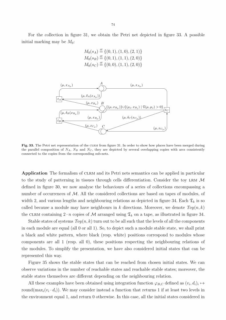
74

For the collection in figure 31, we obtain the Petri net depicted in figure 33. A possible

initial marking may be M0:

M0(sA)df= (0, 1), (1, 0), (2, 1)

M0(sB)df= (0, 1), (1, 1), (2, 0)

M0(sC)df= (0, 0), (1, 1), (2, 0)

A

B

C

tA

tB

tC(µ, xBµ)∪(µj , xBj ) | T(µ, µj) > 0

(µ, xBµ)

(µ, xAµ)

(µ, δA(xAµ))

(µ, xCµ)

(µ, δB(xBµ))

(µ, xBµ)

(µ, xAµ)

(µ, δC(xCµ))

(µ, xCµ)

Fig. 33. The Petri net representation of the clrm from figure 31. In order to show how places have been merged duringthe parallel composition of NA, NB and NC , they are depicted by several overlapping copies with arcs consistentlyconnected to the copies from the corresponding sub-nets.

Application The formalism of clrm and its Petri nets semantics can be applied in particular

to the study of patterning in tissues through cells differentiation. Consider the toy lrm Mdefined in figure 30, we now analyse the behaviours of a series of collections encompassing a

number of occurrences of M. All the considered collections are based on tapes of modules, of

width 2, and various lengths and neighbouring relations as depicted in figure 34. Each Tk is so

called because a module may have neighbours in k directions. Moreover, we denote Toy(n, k)

the clrm containing 2 · n copies ofM arranged using Tk on a tape, as illustrated in figure 34.

Stable states of systems Toy(n, k) turn out to be all such that the levels of all the components

in each module are equal (all 0 or all 1). So, to depict such a module stable state, we shall print

a black and white pattern, where black (resp. white) positions correspond to modules whose

components are all 1 (resp. all 0), these positions respecting the neighbouring relations of

the modules. To simplify the presentation, we have also considered initial states that can be

represented this way.

Figure 35 shows the stable states that can be reached from chosen initial states. We can

observe variations in the number of reachable states and reachable stable states; moreover, the

stable states themselves are different depending on the neighbouring relation.

All these examples have been obtained using integration function ϕB,C defined as (vi, di)i 7→round(maxi(vi · di)). We may consider instead a function that returns 1 if at least two levels in

the environment equal 1, and return 0 otherwise. In this case, all the initial states considered in

75

T4(i, j)df= T4(j, i)

df=

1 if j = i+ 2 ∨ (i mod 2 = 0 ∧ j = i+ 1)0 otherwise

0

1

2

3

4 · · ·

5 · · ·

T8(i, j)df= T8(j, i)

df=

1 if j = i+ 1 ∨ j = i+ 2 ∨ (i mod 2 = 0 ∧ j = i+ 3)0 otherwise

0

1

2

3

4 · · ·

5 · · ·

T6(i, j)df= T6(j, i)

df=

1 if j = i+ 1 ∨ j = i+ 20 otherwise

0

1

2

3

4 · · ·

5 · · ·

Fig. 34. The various neighbouring relations considered for 2-width tapes. On the left, the graphical view showing theorganisation of the connexions. Definitions of the corresponding neighbouring relations on the right side rely on theassumption that modules on the top line of the tape are numbered with consecutive even numbers, while modules on thebottom line are numbered (following the same direction) with consecutive odd numbers.

figure 35 for Toy(2, 4), Toy(3, 4) and Toy(4, 4) become stable states. This shows that the choice

of integration functions have an influence on the systems as well as the choice of neighbouring

relations.

Related works Among the diversity of modelling frameworks used to model regulatory net-

works (see [42, 130] for surveys), the logical approach, initially developed by R. Thomas and

co-workers [135, 136], is a successful qualitative formalism. It has been applied to model and

analyse regulatory networks controlling a variety of cellular processes from pattern formation

and cell differentiation [128, 129, 88] to cell cycle [59], including regulatory networks comprising

relatively large numbers of components [126, 127].

Various Petri net semantics of logical regulatory graphs have been defined, using either p/t

nets or coloured Petri nets [31, 32]. The global idea of these semantics is to represent the value of

a regulatory component by an integer-valued token in a place (or by several black tokens in one

place and its complementary place in the case of p/t nets). Then, the possible evolutions of each

component are encoded as transitions that update the encoded value of the component while

testing the value of other components in order to ensure that evolutions are actually allowed

at a given state. The approach proposed in [134] is quite similar but additional constructs are

used to enforce a synchronous semantics of the modelled networks, i.e., a simultaneous update

of all the regulation components. In terms of Petri nets, this amount to implement a maximal

step semantics, which is done in [134] through a two-phases update process: the first phase

identifies all the components that are called to change their value, the second phase performs

this update synchronously.

With respect to these Petri nets semantics, our approach follows the same principles but

produces more compact Petri nets by folding into a unique place and a unique transition all

the information and logic for each regulatory component. Moreover, this Petri net is obtained

76

Toy(2, 4) 1 reachable state (1 stable)

Toy(2, 8) 64 reachable states (3 stable)

Toy(2, 6) 64 reachable states (3 stable)

Toy(3, 4) 54 reachable states (3 stable)

Toy(3, 8) 512 reachable states (5 stable)

Toy(3, 6) 512 reachable states (5 stable)

Toy(4, 4) 64 reachable states (3 stable)

Toy(4, 8) 4096 reachable states (8 stable)

Toy(4, 6) 512 reachable states (5 stable)

Fig. 35. The reachable stable states for the considered Toy(n, k). Each row indicates on the left the considered modeland its initial state; on the right are indicated the total number of reachable states among which the stable ones aredepicted. The top-left module of each state is decorated with links showing the directions of its potential neighbours.

77

in a structured way which is much easier to implement (and less error prone). In our snakes-

based implementation, each lrm is defined as a Python class whose methods implement the

logical functions from K; a clrm is obtained by instantiating such classes and providing the

neighbouring information. This way, the Petri net needed for the analysis is derived from a tex-

tual specification in a fully automated way, without any requirement to manipulate regulatory

graphs.

6 Conclusion

We have presented a modular framework of coloured Petri nets with various modelling features

(see also figure 36):

– the core of the framework is a general class of coloured Petri nets that is not tied to any

specific colour domain;

– by adding statuses to the places, we have defined Petri nets with control flow that introduce

explicit asynchronous communication through named places and four control flow composi-

tions (sequence, parallel, iteration and choice);

– by adding multi-actions to the transitions, we have defined Petri nets with synchronisa-

tion that provide with an explicit mechanism of multi-way transitions synchronisation with

argument passing;

– by removing parallel composition from Petri nets with control flow and adding an exception

control flow as white tokens in addition to black tokens, we have defined Petri nets with

exceptions allowing to model a full-featured exception mechanism;

– finally, by defining a task construction operator and a distributed scheme for process iden-

tifier generation, we have defined Petri nets with threads allowing to define dynamic thread

creations and function calls.

implementedin snakes

coloured Petri nets

Petri nets with control flowabcd Petri nets with synchronisation

Petri nets with exceptions

Petri nets with threads

Fig. 36. The structure of our framework.

The snakes toolkit that implement part of this framework has been presented. snakes

itself is designed to be flexible and modular thanks to a built-in plugin system.

Models based on this framework have been applied to various domains. We have presented

an approach to the modelling of timed systems by implementing clocks as counters of a tick

78

transition occurrences. Then we have illustrated how the abcd syntax, defined on the top

of Petri nets with control flow, can be used to specify and verify security protocols with a

mixture of symbolic treatment and Python implementation of the cryptographic features. A

third application has been to define a modular formalism for modelling regulation between

biological entities (e.g., cells), taking into account their neighbouring relations. This has been

used to study patterning mechanisms in the context of developmental processes.

On the way, we have identified specific verification issues and proposed solutions to improve

the efficiency of verification:

– using a compilation approach, a coloured Petri nets can be implemented as a software

library that can be used for model-checking the Petri net of interest. Doing so, it is possible

to introduce specific optimisations at many levels by taking advantage of the structure and

properties of the compiled Petri net;

– moreover, when a Petri net is constructed by compositions, structural information can be

derived automatically and used to improve the verification or to introduce more optimisation

in the compilation. This kind of information can also be exploited to improve the parallel

computation of the reachability graph of a Petri net;

– the generation scheme proposed for threads identifiers allows to define a method to deal with

symmetric executions of a multi-threaded system, or infinite repetitions with varying thread

identifiers. This method is based on a general behaviour-preserving marking equivalence

that can be implemented has a graph isomorphism check, and we could show that this test

is efficient in practice;

– the modelling of time by causality introduces counters of ticks that accelerate the state

explosion problem and possibly lead to infinite state space. We have shown how counters

can be implemented aside the Petri net using a dedicated library. By using a detection of

cycles in the behaviour, large or infinite state spaces can be compressed to a storage-efficient

over-approximation that is suitable for reachability analysis.

6.1 Ongoing and future works

The framework presented in this document is still under active development, several tasks have

been already started and others are planned. In the following, we use one to three stars to

denote: ongoing and short-term tasks (?), medium-term tasks (??), or long-term projects (???).

First, a Master thesis has just finished (?) about improving the modelling of topological

aspects in the bio-informatics application, including the possibility of cells migration, replication

and apoptosis (death). The idea is to maintain, aside the Petri net that encode the logic of

regulatory components, a structure to encode the neighbourhood relationship; this is made

in such a way that the topology can be queried from the Petri net, for instance to retrieve

information or require a topological change. For this purpose, we use the tool mgs that can

model in a flexible way very general topological collections [91, 90]. Finally, approach to model

79

patterning mechanism described above for a toy example is being applied to study the segment-

polarity module involved in the segmentation of the Drosophilia embryo (?).

Next, work is planned to implement the full framework in snakes, in particular Petri

nets with exceptions and Petri nets with threads (??). This should lead to extend the abcd

language to support these features (??). snakes will also be extended to support version 3 of the

pnml standard [106] that defines the representation of coloured Petri nets (?). The compilation

approach for faster verification presented in section 2.5 has been developed by a Master student

who has implemented a prototype. It is planned to integrate this work into snakes to improve

simulation performances (?). On the long term, snakes may be extended to support colour

domains others than the Python language, in particular compiled languages (???). Indeed, by

using the compilation approach, Petri nets can be compiled to native libraries that in turn may

be loaded from Python and thus used by snakes.

This work will also help to support an industrial thesis that will start in December 2009

(???) in the context of project spreads [133] and, among other questions, will address the

problem of interfacing a Petri net with an execution context. The issue here is to formalise the

link between a specification and the corresponding implementation, which is envisaged in two

ways: parts of an existing implementation can be embedded as annotations in a Petri net model

to be verified; conversely, a Petri net model may be integrated to an existing application as a

component. The goal of this approach is to improve the confidence about the implementation

by tightening its relationship with a verified specification.

Several case studies are in progress and more are envisaged to apply our approaches. First,

project spreads [133] will continue until the end of 2010. Currently, a first version of the

protocol involving a central directory server has been modelled and verified using abcd (?).

The next version uses a directory service that is distributed over the network of peers (??).

This is currently being designed, both through the implementation of prototypes and through

abcd modelling, verification and simulation. Another case study in progress is about a non-

repudiation protocol that involves complex control-flow to model alternative and repetitive

behaviours of a server, and the possibility of timeouts on the clients side. This protocol is being

modelled using abcd to verify its properties. This work is in its early stages but a paper is

planned on the subject (?). It is also planned to run several case studies concerning causal time

to consolidate our results and extend the approach if necessary (??).

Concerning verification, the PhD thesis about parallel computing is still in progress. We

expect results by the end of the PhD that is planned in October 2010. On the short term, several

algorithms have been designed and benchmarked, the resulting raw measures are being analysed

in order to draw conclusions about their comparative performances (?). Moreover, we envisage

to study how the verification methods we proposed can be combined. In particular, combining

the compact state space abstraction of Petri nets with counters with the marking equivalence

for Petri nets with threads seems particularly challenging and in the same time interesting for

80

many applications (???). On the other hand, combining the compilation approach with other

techniques is expected to be quite straightforward (??).

Several other ways are envisaged to improve the verification of our models. First, a work

has been started to adapt the sweep-line method [34, 83] in the context of security protocol

models (?). Indeed, this method relies on a measure of progression in the analysed system: each

computed state s is associated a measure ψ(s) from an ordered set in a way that is compatible

with the reachability relation (i.e., if state s′ is reachable from state s then we should have

ψ(s′) ≥ ψ(s)). The principle of the sweep-line method is to process states in growing order

and dispose from memory the states that cannot be reached again according to the measure.

The difficulty with this method is usually to define a non-trivial measure that is fine enough

to really lower memory consumption. In the context of security protocols where agents have

sequential behaviours, we can observe their control-flow state to measure their progression. A

very fine-grain measure can thus be automatically derived from the model and used to save

memory, allowing to analyse complex scenarios with huge state spaces.

Other ways of exploiting the structure of the analysed models are envisaged as future works.

In particular, modular verification [35, 87] relies on a decomposition of the model into a hierarchy

of sub-models. Such a decomposition is usually not available and has to be defined by the user of

the tool. But since our models are build by compositions, we have natural knowledge about their

structure, which should be exploitable to derive automatically a sensible decomposition that

is suitable for modular verification (???). A similar approach should be applicable to encode

efficiently the state spaces of our models into hierarchical decision diagrams as defined in [61,

23] and implemented in alpina [3] (???). Indeed, a good ordering of variables is known to

be a key issue to achieve good compression using decision diagrams, and this question is even

more crucial and more complex at the same time when hierarchical diagrams are considered.

Here also, our knowledge of the structure of the analysed model should be exploitable to derive

automatically sensible ordering and hierarchy of the variables needed to encode states. We

expect to achieved very good compression on systems with many regularities, in particular

systems with duplicated components (like models of protocols with several instances of an

agent), multi-threaded systems (with several instances of a task), or systems with many similar

tokens like models of biological regulatory networks.

81

References

1. Martın Abadi and Andrew D. Gordon. A calculus for cryptographic protocols: the spi calculus. In CCS’97. ACM,1997.

2. Olga Marroquın Alonso and David de Frutos Escrig. Extending the Petri box calculus with time. In ICATPN’01,volume 2075 of LNCS. Springer, 2001.

3. AlPiNA: an algebraic Petri net analyzer. 〈http://alpina.unige.ch〉.4. Rajeev Alur and David L. Dill. A theory of timed automata. Theoretical Computer Science, 126(2), 1994.5. The ASCoVeCo project. 〈http://www.daimi.au.dk/~ascoveco〉.6. AVISPA: Automated validation of Internet security protocols and applications. 〈http://avispa-project.org〉.7. Sebastien Bardin, Alain Finkel, Jerome Leroux, and Laure Petrucci. FAST: Fast acceleration of symbolic transition

systems. In CAV’03, volume 2725 of LNCS. Springer, 2003.8. Sebastien Bardin and Laure Petrucci. From PNML to counter systems for accelerating Petri nets with FAST. In

Ekkart Kindler, editor, Workshop on Definition, Implementation and Application of a Standard Interchange Formatfor Petri Nets, Universitat Paderborn, Germany, 2004.

9. J. A. Bergstra, A. Ponse, and Scott A. Smolka, editors. Handbook of Process Algebra. Elsevier, 2001.10. Eike Best and Raymond Devillers. Sequential and concurrent behaviour in Petri net theory. Theoretical Computer

Science, 55(1), 1987.11. Eike Best, Raymond Devillers, and Jon G. Hall. The box calculus: a new causal algebra with multi-label commu-

nication. In Advances in Petri Nets 1992, The DEMON Project. Springer, 1992.12. Eike Best, Raymond Devillers, and Maciej Koutny. Petri net algebra. Springer, 2001.13. Eike Best, Wojciech Fraczak, Richard P. Hopkins, Hanna Klaudel, and Elisabeth Pelz. M-nets: An algebra of

high-level Petri nets, with an application to the semantics of concurrent programming languages. Acta Informatica,35(10), 1998.

14. Eike Best and Richard P. Hopkins. B(PN)2 – a basic Petri net programming notation. In PARLE’93. Springer,1993.

15. Bruno Blanchet. An efficient cryptographic protocol verifier based on Prolog rules. In IEEE CSFW’01. IEEEComputer Society, 2001.

16. Yohan Boichut, Pierre-Cyrille Heam, and Olga Kouchnarenko. Handling algebraic properties in automatic analysisof security protocols. In ICTAC’06, volume 4281 of LNCS. Springer, 2006.

17. Bernard Boigelot. The Liege automata-based symbolic handler. 〈http://www.montefiore.ulg.ac.be/~boigelot/research/lash〉.

18. Dragan Bosnacki, Dennis Dams, and Leszek Holenderski. Symmetric Spin. International Journal Software Toolsfor Technology Transfer, 4(1), 2002.

19. Cherif Boukala and Laure Petrucci. Towards distributed verification of Petri nets properties. In VECOS’07, eWiC.British Computer Society, 2007.

20. Roland Bouroulet, Raymond Devillers, Hanna Klaudel, Elisabeth Pelz, and Franck Pommereau. Modeling andanalysis of security protocols using role based specifications and Petri nets. In ICATPN’08, volume 5062 of LNCS,pages 72–91. Springer, 2008.

21. Roland Bouroulet, Hanna Klaudel, and Elisabeth Pelz. A semantics of security protocol language (SPL) using aclass of composable high-level Petri nets. In ACSD’04. IEEE Computer Society, 2004.

22. Roland Bouroulet, Hanna Klaudel, and Elisabeth Pelz. Modelling and verification of authentication using enhancednet semantics of SPL (security protocol language). In ACSD’06. IEEE Computer Society, 2006.

23. Didier Buchs and Steve Hostettler. Managing complexity in model checking with decision diagrams for algebraicpetri net. In Daniel Moldt, editor, Pre-proceedings of PNSE’09, 2009.

24. Cecile Bui Thanh. Generating coloured Petri nets of concurrent object-oriented programs. In ESMc’04. EUROSIS,2004.

25. Cecile Bui Thanh, Hanna Klaudel, and Franck Pommereau. Box calculus with coloured buffers. Technical Report 16,LACL, University Paris East, 2002.

26. Cecile Bui Thanh, Hanna Klaudel, and Franck Pommereau. Petri nets with causal time for system verification. InMTCS’02, volume 68(5) of ENTCS, pages 1–16. Elsevier, 2003.

27. Cecile Bui Thanh, Hanna Klaudel, and Franck Pommereau. Box calculus with high-level buffers. In DADS’04,pages 1–6. SCS, 2004.

28. Beatrice Berard, Michel Bidoit, Alain Finkel, Francois Laroussinie, Antoine Petit, Laure Petrucci, and PhilippeSchnoebelen. Systems and software verification: model-checking techniques and tools. Springer, 2001.

29. Claudine Chaouiya, Hanna Klaudel, and Franck Pommereau. A Petri net based framework for a qualitative mod-elling of regulatory networks encompassing inter-cellular signalling. In Arcadi Navarro and Arlindo Oliveira, editors,JB’09, pages 1–5, 2009.

30. Claudine Chaouiya, Hanna Klaudel, and Franck Pommereau. Qualitative modelling of regulatory networks usingPetri nets: application to developmental processes, chapter in preparation. Ina Koch, editor. Springer, to appear.

31. Claudine Chaouiya, Elisabeth Remy, Paul Ruet, and Denis Thieffry. Qualitative modelling of genetic networks:From logical regulatory graphs to standard Petri nets. In ICATPN’04, volume 3099 of LNCS. Springer, 2004.

32. Claudine Chaouiya, Elisabeth Remy, and Denis Thieffry. Qualitative Petri net modelling of genetic networks.TCSB, VI(4220), 2006.

82

33. Giovanni Chiola, Claude Dutheillet, Giuliana Franceschinis, and Serge Haddad. On well-formed coloured nets andtheir symbolic reachability graph. In High-Level Petri Nets – Theory and Application. Springer, 1991.

34. Søren Christensen, Lars Michael Kristensen, and Thomas Mailund. A sweep-line method for state space exploration.In TACAS’01, volume 2031 of LNCS. Springer, 2001.

35. Søren Christensen and Laure Petrucci. Modular analysis of Petri nets. The Computer Journal, 43(3), 2000.36. Edmund M. Clarke, E. Allen Emerson, Somesh Jha, and A. Prasad Sistla. Symmetry reductions in model checking.

In CAV’98, volume 1427 of LNCS. Springer, 1998.37. Luigi P. Cordella, Pasquale Foggia, Carlo Sansone, and Mario Vento. A (sub)graph isomorphism algorithm for

matching large graphs. IEEE Transactions on Pattern Analysis and Machine Intelligence, 26(10), 2004.38. Jean-Michel Couvreur. A BDD-like implementation of an automata package. In CIAA’04, volume 3317 of LNCS.

Springer, 2004.39. Jean-Michel Couvreur, Emmanuelle Encrenaz, Emmanuel Paviot-Adet, Denis Poitrenaud, and Pierre-Andre Wacre-

nier. Data decision diagrams for Petri net analysis. In ICATPN’02. Springer, 2002.40. CPN Group, University of Aarhus. CPN Tools. 〈http://wiki.daimi.au.dk/cpntools〉.41. Federico Crazzolara and Glynn Winskel. Events in security protocols. In CCS’01. ACM, 2001.42. Hidde de Jong. Modeling and simulation of genetic regulatory systems: a literature review. Journal of Computational

Biology, 1(9), 2002.43. Raymond Devillers, Hanna Klaudel, Maciej Koutny, Elisabeth Pelz, and Franck Pommereau. Operational semantics

for PBC with asynchronous communication. In HPC’02, pages 1–6. SCS, 2002.44. Raymond Devillers, Hanna Klaudel, Maciej Koutny, and Franck Pommereau. An algebra of non-safe Petri boxes.

In AMAST’02, volume 2422 of LNCS, pages 185–214. Springer, 2002.45. Raymond Devillers, Hanna Klaudel, Maciej Koutny, and Franck Pommereau. Asynchonous box calculus. Funda-

menta Informaticae, 54(1):1–50, 2003.46. Raymond R. Devillers, Hanna Klaudel, and Robert-C. Riemann. General parameterised refinement and recursion

for the M-net calculus. Theoretical Compututer Science, 300(1–3), 2003.47. Whitfield Diffie and Martin Hellman. New directions in cryptography. IEEE Transactions on Information Theory,

22(6), 1976.48. Danny Dolev and Andrew Yao. On the security of public key protocols. IEEE Transactions on Information Theory,

29(2), 1983.49. Hartmut Ehrig and Bernd Mahr. Fundamentals of Algebraic Specification I. Springer, 1985.50. Jacob Elgaard, Nils Klarlund, and Anders Møller. MONA 1.x: new techniques for WS1S and WS2S. In CAV’98,

volume 1427 of LNCS. Springer, 1998.51. John Ellson, Emden R. Gansner, Eleftherios Koutsofios, Stephen C. North, and Gordon Woodhull. Graphviz - open

source graph drawing tools. In Graph Drawing’01, volume 2265 of LNCS. Springer, 2001.52. Javier Esparza and Mogens Nielsen. Decidability issues for Petri nets–A survey. Bulletin of the European Association

for Theoretical Computer Science, 52, 1994.53. Javier Esparza, Stefan Romer, and Walter Vogler. An improvement of McMillan’s unfolding algorithm. In FMSD’96.

Springer, 1996.54. Sami Evangelista, Serge Haddad, and Jean-Francois Pradat-Peyre. New coloured reductions for software validation.

In WODES’04, 2004.55. Sami Evangelista, Serge Haddad, and Jean-Francois Pradat-Peyre. Syntactical colored Petri nets reductions. In

ATVA’05, volume 3707 of LNCS. Springer, 2005.56. Sami Evangelista and Jean-Francois Pradat-Peyre. An efficient algorithm for the enabling test of colored Petri nets.

In CPN’04, number 570 in DAIMI report PB. University of Arhus, Denmark, 2004.57. Sami Evangelista and Jean-Francois Pradat-Peyre. Memory efficient state space storage in explicit software model

checking. In SPIN’05, volume 3639 of LNCS. Springer, 2005.58. Sami Evangelista and Jean-Francois Pradat-Peyre. On the computation of stubborn sets of colored Petri nets. In

ICATPN’06, volume 4024 of LNCS. Springer, 2006.59. Adrien Faure, Aurelien Naldi, Claudine Chaouiya, and Denis Thieffry. Dynamical analysis of a generic Boolean

model for the control of the mammalian cell cycle. Bioinformatics, 22(14), 2006.60. Aric A. Hagberg, Daniel A. Schult, and Pieter J. Swart. Exploring network structure, dynamics, and function using

NetworkX. In SciPy’08. 〈http://conference.scipy.org〉, 2008.61. Alexandre Hamez, Yann Thierry-Mieg, and Fabrice Kordon. Hierarchical set decision diagrams and automatic

saturation. In ICATPN’08. Springer, 2008.62. Keijo Heljanko, Victor Khomenko, and Maciej Koutny. Parallelisation of the Petri net unfolding algorithm. In

TACAS’02, volume 2280 of LNCS. Springer, 2002.63. Martijn Hendriks, Gerd Behrmann, Kim Guldstrand Larsen, Peter Niebert, and Frits W. Vaandrager. Adding

symmetry reduction to Uppaal. In FORMATS’03, volume 2791 of LNCS. Springer, 2003.64. Gerard J. Holzmann. An analysis of bitstate hashing. Formal Methods in System Design, 13(3), 1998.65. Gerard J. Holzmann and al. Spin, formal verification. 〈http://spinroot.com〉.66. C. Norris Ip and David L. Dill. Better verification through symmetry. Formal Methods in System Design, 9(1–2),

1996.67. Kurt Jensen and Lars M. Kristensen. Coloured Petri Nets: Modelling and Validation of Concurrent Systems.

Springer, 2009.

83

68. Tommi Junttila. On the Symmetry Reduction Method for Petri Nets and Similar Formalisms. PhD thesis, HelsinkiUniversity of Technology, Laboratory for Theoretical Computer Science, Espoo, Finland, 2003.

69. Jens B. Jørgensen and Lars M. Kristensen. Verification of coloured Petri nets using state spaces with equivalenceclasses. LINCOM Studies in Computer Science, 1, 2003.

70. Victor Khomenko. Punf: Petri net unfolder. 〈http://homepages.cs.ncl.ac.uk/victor.khomenko/tools/punf〉.71. Victor Khomenko. Model Checking Based on Prefixes of Petri Net Unfoldings. PhD thesis, School of Computing

Science, Newcastle University, Newcastle upon Tyne, GB, 2003.72. Kais Klai, Laure Petrucci, and Michel Reniers. An incremental and modular technique for checking LTL\X prop-

erties of Petri nets. In FORTE’07. Springer, 2007.73. Hanna Klaudel. Parameterized M-expression semantics of parallel procedures. In DAPSYS’00. Kluwer Academic

Publishers, 2000.74. Hanna Klaudel, Maciej Koutny, Elisabeth Pelz, and Franck Pommereau. Towards efficient verification of systems

with dynamic process creation. In ICTAC’08, volume 5160 of LNCS, pages 186–200. Springer, 2008.75. Hanna Klaudel, Maciej Koutny, Elisabeth Pelz, and Franck Pommereau. Towards efficient verification of systems

with dynamic process creation. Technical Report 8, LACL, University Paris East, 2008.76. Hanna Klaudel, Maciej Koutny, Elisabeth Pelz, and Franck Pommereau. An approach to state space reduction for

systems with dynamic process creation. In ISCIS’09, pages 1–6. IEEE Computer Society, to appear.77. Hanna Klaudel and Franck Pommereau. Asynchronous links in the PBC and M-nets. In ASIAN’99, volume 1742

of LNCS, pages 190–200. Springer, 1999.78. Hanna Klaudel and Franck Pommereau. A concurrent and compositional Petri net semantics of preemption. In

IFM’00, volume 1945 of LNCS, pages 318–337. Springer, 2000.79. Hanna Klaudel and Franck Pommereau. A concurrent semantics of static exceptions in a parallel programming

language. In ICATPN’01, volume 2075 of LNCS, pages 204–223. Springer, 2001.80. Hanna Klaudel and Franck Pommereau. A class of composable and preemptible high-level Petri nets with an

application to multi-tasking systems. Fundamenta Informaticae, 50(1):33–55, 2002.81. Hanna Klaudel and Franck Pommereau. M-nets: a survey. Acta Informatica, 45(7–8):537–564, 2009.82. Maciej Koutny. A compositional model of time Petri nets. In ICATPN’00, volume 1825 of LNCS. Springer, 2000.83. Lars Michael Kristensen and Thomas Mailund. A generalised sweep-line method for safety properties. In

FME/FM’02, volume 2391 of LNCS. Springer, 2002.84. Flavio Lerda and Riccardo Sisto. Distributed-memory model checking with Spin. In SPIN’99. Springer, 1999.85. Glenn Lewis and Charles Lakos. Incremental state space construction for coloured Petri nets. In ICATPN’01.

Springer, 2001.86. Kenneth L. MacMillan. Symbolic Model Checking. Kluwer Academic Publishers, 1993.87. Marko Makela. Maria: Modular reachability analyser for algebraic system nets. In ICATPN’02, volume 2360 of

LNCS. Springer, 2002.88. Luis Mendoza. A network model for the control of the differentiation process in Th cells. Biosystems, 84(2), 2006.89. Philip M. Merlin and David J. Farber. Recoverability of communication protocols: Implications of a theoretical

study. IEEE Transaction on Communications, 24(9), 1976.90. Olivier Michel. There is plenty of room for unconventional programming languages or declaratives simulations of

dynamicals systems (with a dynamical structure). Habilitation Thesis, IBISC, University of Evry, 2007.91. Olivier Michel, Jean-Louis Giavitto, Julien Cohen, and Antoine Spicher. MGS. 〈http://mgs.ibisc.univ-evry.fr〉.92. Alice Miller, Alastair Donaldson, and Muffy Calder. Symmetry in temporal logic model checking. ACM Computing

Surveys (CSUR), 38(3), 2006.93. Robin Milner. Communicating and Mobile Systems: the Pi-Calculus. Cambridge University Press, 1999.94. Marko Makela. Maria: The modular reachability analyzer. 〈http://www.tcs.hut.fi/Software/maria〉.95. Marko Makela. Applying compiler techniques to reachability analysis of high-level models. In Hans-Dieter Burkhard,

Ludwik Czaja, Andrzej Skowron, and Peter Starke, editors, CS&P’00, number 140 in Informatik-Bericht. Humboldt-Universitat zu Berlin, Germany, 2000.

96. Marko Makela. Condensed storage of multi-set sequences. In Kurt Jensen, editor, CPN’00, number 547 in DAIMIreport PB. University of Arhus, Denmark, 2000.

97. Marko Makela. Optimising enabling tests and unfoldings of algebraic system nets. In ICATPN’01, volume 2075 ofLNCS. Springer, 2001.

98. Marko Makela. A reachability analyser for algebraic system nets. Research Report A69, Helsinki University ofTechnology, Laboratory for Theoretical Computer Science, 2001.

99. Roger M. Needham and Michael D. Schroeder. Using encryption for authentication in large networks of computers.Communication of the ACM, 21(12), 1978.

100. Christophe Pajault and Sami Evangelista. Helena: a high level net analyzer. 〈http://helena.cnam.fr〉.101. Christophe Pajault and Jean-Francois Pradat-Peyre. Distributed colored Petri net model-checking with Cyclades.

In FMICS/PDMC’06, volume 4346 of LNCS. Springer, 2006.102. Parallel Systems Group, University of Oldenburg. The PEP tool. 〈http://peptool.sourceforge.net〉.103. Elisabeth Pelz and Dietmar Tutsch. Formal models for multicast traffic in network on chip architectures with

compositional high-level Petri nets. In ICATPN’07, volume 4546 of LNCS. Springer, 2007.104. James L. Peterson. Petri nets. ACM Computing Surveys, 9(3), 1977.105. James Lyle Peterson. Petri Net Theory and the Modeling of Systems. Prentice Hall PTR, 1981.

84

106. Petri net markup language. 〈http://www.pnml.org〉.107. Franck Pommereau. SNAKES is the net algebra kit for editors and simulators. 〈http://lacl.univ-paris12.fr/

pommereau/soft/snakes〉.108. Franck Pommereau. FIFO buffers in tie sauce. In DAPSYS’00, pages 95–104. Kluwer Academic Publishers, 2000.109. Franck Pommereau. Modeles composables et concurrents pour le temps-reel. PhD thesis, LACL, University Paris

East, 2002.110. Franck Pommereau. Causal time calculus. In FORMATS’03, volume 2791 of LNCS, pages 1–12. Springer, 2003.111. Franck Pommereau. Petri nets as executable specifications of high-level timed parallel systems. In PAPP/ICCS’04,

volume 3038 of LNCS, pages 331–338. Springer, 2004.112. Franck Pommereau. Versatile boxes: a multi-purpose algebra of high-level Petri nets. In DADS’07, pages 665–672.

SCS/ACM, 2004.113. Franck Pommereau. Petri nets as executable specifications of high-level timed parallel systems. Scalable Computing:

Practice and Experience, 6(6):71–82, 2005.114. Franck Pommereau. Quickly prototyping Petri nets tools with SNAKES. In PNTAP’08, ACM Digital Library,

pages 1–10. ACM, 2008.115. Franck Pommereau. Quickly prototyping Petri nets tools with SNAKES. Petri net newsletter, pages 1–18, 2008.116. Franck Pommereau. Nets-in-nets with SNAKES. In Michael Duvigneau and Daniel Moldt, editors, MOCA’09,

pages 107–126. Universitat Hamburg, Dept. Informatik, 2009.117. Franck Pommereau, Raymond Devillers, and Hanna Klaudel. Efficient reachability graph representation of Petri

nets with unbounded counters. In INFINITY’07, volume 239 of ENTCS, pages 1–10. Elsevier, 2009.118. Franck Pommereau and Christian Stehno. FIFO buffers is hot tie sauce. Technical Report 04, LACL, University

Paris East, 2001.119. William Pugh. The Omega test: a fast and practical integer programming algorithm for dependence analysis. In

ACM/IEEE SC’91. ACM, 1991.120. Python Software Foundation. Python programming language. 〈http://www.python.org〉.121. Michael O. Rabbin. Decidability of second-order theories and automata on infinite trees. Transactions of the AMS,

141, 1969.122. Chandler Ramchandani. Analysis of Asynchronous Concurrent Systems by Timed Petri Nets. PhD thesis, MIT,

Department of Electrical Engineering, Cambridge, Massachusset, USA, 1974.123. Klaus Reinhardt. Reachability in Petri nets with inhibitor arcs. ENTCS, 223, 2008.124. Claus Reinke. Haskell-coloured Petri nets. In IFL’99. Springer, 2000.125. Research Group Petri Net Technology, Humboldt Universitat of Berlin. The Petri net kernel. 〈http://www.

informatik.hu-berlin.de/top/pnkn〉.126. Julio Saez-Rodriguez, Luca Simeoni, Jonathan A Lindquist, Rebecca Hemenway, Ursula Bommhardt, Boerge Arndt,

Utz-Uwe Haus, Robert Weismantel, Ernst D Gilles, Steffen Klamt, and Burkhart Schraven. A logical model providesinsights into T cell receptor signaling. PLoS Computational Biology, 3, 2007.

127. Lucas Sanchez, Claudine Chaouiya, and Denis Thieffry. Segmenting the fly embryo: a logical analysis of the segmentpolarity cross-regulatory module. The International Journal of Developmental Biology, 52(8), 2008.

128. Lucas Sanchez and Denis Thieffry. A logical analysis of the drosophila gap-gene system. Journal of TheoreticalBiology, 211(2), 2001.

129. Lucas Sanchez and Denis Thieffry. Segmenting the fly embryo: a logical analysis of the pair-rule cross-regulatorymodule. Journal of Theoretical Biology, 224(4), 2003.

130. Thomas Schlitt and Alvis Brazma. Current approaches to gene regulatory network modelling. BMC Bioinformatics,8(Suppl 6), 2007.

131. David B. Skillicorn, Jonathan M. D. Hill, and William F. McColl. Questions and answers about BSP. ScientificProgramming, 6(3), 1997.

132. Security protocols open repository. 〈http://www.lsv.ens-cachan.fr/Software/spore〉.133. ANR project SPREADS. 〈http://www.spreads.fr〉, 2007–2010.134. L. Jason Steggles, Richard Banks, Oliver Shaw, and Anil Wipat. Qualitatively modelling and analysing genetic

regulatory networks: a Petri net approach. Bioinformatics, 23(3), 2007.135. Rene Thomas. Boolean formalisation of genetic control circuits. Journal of Theoretical Biology, 42, 1973.136. Rene Thomas, Denis Thieffry, and Marcelle Kaufman. Dynamical behaviour of biological regulatory networks–

I. Biological role of feedback loops and practical use of the concept of the loop-characteristic state. Bulletin ofmathematical Biology, 57(57), 1995.

137. Rudiger Valk. Object Petri nets: Using the nets-within-nets paradigm. In Advanced course on Petri nets, volume3098 of LNCS, pages 819–848. Springer, 2003.