Draft version June 13, 2016Preprint typeset using LATEX style AASTeX6 v. 1.0

THE PROPERTIES OF HEAVY ELEMENTS IN GIANT PLANET ENVELOPES

Francois Soubiran1 and Burkhard Militzer1,2

1Department of Earth and Planetary Science, University of California, Berkeley, CA 94720, United States

and2Department of Astronomy, University of California, Berkeley, CA 94720, United States

ABSTRACT

The core accretion model for giant planet formation suggests a two layer picture for the initial structure

of Jovian planets, with heavy elements in a dense core and a thick H-He envelope. Late planetesimal

accretion and core erosion could potentially enrich the H-He envelope in heavy elements, which is

supported by the three-fold solar metallicity that was measured in Jupiter’s atmosphere by the Galileo

entry probe. In order to reproduce the observed gravitational moments of Jupiter and Saturn, models

for their interiors include heavy elements, Z, in various proportions. However, their effect on the

equation of state of the hydrogen-helium mixtures has not been investigated beyond the ideal mixing

approximation. In this article, we report results from ab initio simulations of fully interacting H-He-Z

mixtures in order to characterize their equation of state and to analyze possible consequences for the

interior structure and evolution of giant planets. Considering C, N, O, Si, Fe, MgO and SiO2, we show

that the behavior of heavy elements in H-He mixtures may still be represented by an ideal mixture

if the effective volumes and internal energies are chosen appropriately. In the case of oxygen, we also

compute the effect on the entropy. We find the resulting changes in the temperature-pressure profile

to be small. A homogeneous distribution of 2% oxygen by mass changes the temperature in Jupiter’s

interior by only 80 K.

Keywords: Physical Data and Processes: equation of state; planets and satellites: gaseous planets;

planets and satellites: Jupiter, Saturn, Uranus, Neptune.

1. INTRODUCTION

Despite numerous observations of giant planets in our

solar system (Bolton 2010; Jones et al. 2015) and the

extrasolar campaigns (Wright et al. 2011; Schneider et

al. 2011), our understanding of the structure, evolu-

tion, and formation of Jovian planets remains uncertain

(Guillot & Gautier 2015). Largely, the uncertainty is

due to the fact that the observations of Jovian planets

only provide data on global properties, which limits the

constraints that can be placed on interior properties.

While future observations, such as the Juno mission,

will provide more detailed data, additional constraints

on Jovian interiors can also be gleaned from advances in

numerical simulations (Militzer 2013) and experiments

(Brygoo et al. 2015) on high density matter and the sub-

sequent improvements in planetary models (Nettelmann

et al. 2012; Helled & Guillot 2013; Hubbard & Militzer

2016).

Even in the solar system, the exact composition of the

gaseous giant planets is still not very well constrained

because the composition of the observable atmosphere

is not necessarily representative of the entire planet.

Following the core-accretion hypothesis (Pollack et al.

1996), Jupiter and Saturn were formed by a rapid ac-

cretion of solid material until a critical mass of approx-

imately 10 M⊕ had been reached, which triggers a sub-

stantial gas accretion. Once the envelope is as massive

as the core, it even becomes a run-away accretion that

stops when all the gas in the nebula has disappeared,

after about 10 Myr. This minimum mass of 10 M⊕provides also a lower bound for the average metallic-

ity of Jupiter and Saturn. As the total mass of Jupiter

(resp. Saturn) is 317.8 M⊕ (resp. 95.1 M⊕) (Baraffe et

al. 2010), the minimal metallicity is ZJ = 0.031 (resp.

ZS = 0.105) which is higher than the solar value of

Z� = 0.0149 (Lodders 2003). But this is only a min-

imum value, and for Jupiter, the Galileo entry probe

measured an atmospheric metallicity of 3 times the so-

lar value (Wong et al. 2004) for instance.

The dichotomy between a dense core and a H-He en-

velope is however, at best, only an approximated view of

the giant planets as there are at least five different rea-

sons why the heavy element distribution in giant plan-

ets is uncertain. The first one comes from the forma-

2 Soubiran & Militzer

tion of the planet. During the gas accretion, the planet

kept accreting additional planetesimals and it is unclear

whether they dissolved in the envelope or reached the

core (Fortney et al. 2013).

The second reason is the possible erosion of the core

as proposed by Stevenson (1982), which could trigger a

redistribution of the heavy elements of the core through-

out the envelope. This possibility has been recently in-

vestigated with ab initio simulations, which predicted

that all the dominant species in the core are miscible in

metallic hydrogen (Wilson & Militzer 2012a,b; Wahl et

al. 2013; Gonzalez-Cataldo et al. 2014).

However, and this is the third reason, the kinetics of

the erosion process is very poorly constrained and could

be very slow. Once dissolved in hydrogen, the heavy

elements may not be efficiently redistributed throughout

the envelope because the density contrast may be too

high for the convection to advect these elements against

the gravitational forces. Thus, a semi-convective pattern

is likely to set in, inducing a gradient of composition in

the layers close to the core (Leconte & Chabrier 2012,

2013).

An other origin of heterogeneity in giant planet en-

velopes could come from the phase separation of H-He

which has been proposed as an explanation of the ex-

cess of luminosity of Saturn (Stevenson & Salpeter 1977;

Fortney & Hubbard 2004). The exact phase diagram

is still controversial despite recent work using ab ini-

tio simulations (Lorenzen et al. 2009, 2011) and even

thermodynamic integrations to properly account for the

non-ideal entropy (Morales et al. 2009, 2013). How-

ever, some experimental constraints should be available

shortly using reflectivity measurements in laser-driven

shock experiments (Soubiran et al. 2013). But if the

phase separation occurs in a giant planet, it could also

inhibit the advection of heavy elements from the deep

interior to the external layers as the convection would

most likely be rendered less efficient by the phase sepa-

ration.

The last reason of uncertainty comes from the possible

partitioning of the heavy elements due to the miscibility

difference with helium and with hydrogen. It has been

suggested, for instance, as an explanation for the strong

depletion in neon in the atmosphere of Jupiter (Wilson

& Militzer 2010).

We therefore need to have better constraints on the

distribution of the heavy elements. They may come from

both observations and more detailed models. Measure-

ments of the gravitational field of Jupiter and Saturn via

the study of the trajectory of their satellites but also via

direct measurements from spacecrafts such as Cassini

and Juno can give strong constraints on the gravita-

tional moments of the planet and thus on the mass dis-

tribution. A new field is also emerging: seismology of

Figure 1. Snapshot of a simulation box containing 220 H(white), 18 He (green) and 4 Fe (yellow) atoms at 2000 K and60 GPa. We used a distance analysis to identify the chemicalbonds. The isosurfaces represent the electronic density.

giant planets. Recent results using planetary oscillations

(Gaulme et al. 2011) and more importantly through

ring seismology (Fuller et al. 2014a; Fuller 2014b) have

started to demonstrate its potential and will most likely

lead to additional constraints.

Theorists can also help to constrain the possible struc-

tures by building detailed models including accurate

physical properties of matter at high density. Improve-

ments in ab initio simulations over the past two decades

offered the possibility to compute precise equations of

state (EOS). Recently an updated EOS of H-He has been

developed by Militzer (2013). Concerning the heavy el-

ements, different EOSs have been used in giant planet

models (see Baraffe et al. (2008) for a review of the

common EOSs). Recent models showed that the heavy

elements altered the density profile and therefore the

structure of the planet (Hubbard & Militzer 2016), as

well as its evolution (Baraffe et al. 2008). However,

these models rely on the assumption that the multi-

component mixtures of interest are ideal mixtures with

an isothermal-isobaric additive mixing rule. Under this

assumption, one derives all extensive thermodynamic

properties of a mixture – volume, internal energy,... –

by adding up the contributions from the individual pure

species at a given temperature and pressure. Such a

mixing rule neglects all the inter-species interactions,

although they may be much more important than the

intra-species ones. For instance, in the diluted limit,

a heavy atom only interacts with the H-He – solvent

– atoms while, in the ideal mixing approximation, the

H-He-Z mixtures 3

properties of the heavy species are taken from a system

of heavy atoms only.

Once the Juno mission will have measured the gravi-

tational moments of Jupiter with high precision, interior

models with various amounts of heavy elements in the

envelope and different core sizes will be constructed to

match these measurements. This will improve our un-

derstanding of the interior structure and the evolution

of Jupiter. One goal of this paper is to make this anal-

ysis more accurate by going beyond the standard ideal

mixing rule and by properly characterizing the influence

of heavy elements on a H-He envelope.

In this article, we investigate the thermodynamic

properties of ternary mixtures of hydrogen, helium and

heavy elements – namely carbon, nitrogen, oxygen, sili-

con, iron as well as magnesium oxide and silicon dioxide

– under conditions relevant for the giant planet interiors.

We used ab initio simulations to determine the influence

of these seven elements on the density and the internal

energy. On the case of oxygen, we also studied the influ-

ence on the entropy, which is essential to determine the

pressure-temperature profile in giant planet envelopes.

From our analysis we determined that the ternary

mixtures can indeed be very well described by an ideal

isothermal-isobaric mixing of H-He on one side and the

heavy element on the other, provided however that ef-

fective volume or energy of the heavy species are cho-

sen appropriately. Both properties may differ from the

properties from those of the pure species at the same

temperature and conditions. They may furthermore be

affected by the dissociation of hydrogen.

We also performed entropy calculations for H-He-

O ternary mixtures. We show that the addition of

heavy element, homogeneously throughout the envelope

of a giant planet, has only a marginal influence on the

pressure-temperature and on the density profiles. Last,

we explore the influence of the heavy elements on the

mass-radius relationship of giant planets.

2. SIMULATION METHODS

We performed molecular dynamics (MD) simula-

tions with forces derived from density functional theory

(DFT) (Hohenberg & Kohn 1964) to treat the quan-

tum behavior of the electrons. We performed the sim-

ulations with the Vienna ab initio simulation package

(Kresse & Furthmuller 1996). We used cubic cells with

periodic boundary conditions. Starting from cells with

220 hydrogen and 18 helium atoms (Militzer 2013), we

added from 2 to 8 atoms or molecules of heavy elements

– we considered C, N, O, Si, Fe, MgO and SiO2. As

an example, Fig. 1 shows a representative snapshot of a

simulation of H, He and Fe.

We performed the dynamics with a 0.2 fs time step,

for a trajectory of at least 1 ps. The temperature

101 102 103

Pressure [GPa]

2000

4000

6000

8000

10000

12000

14000

Tem

pera

ture

[K

]

Jupiter

Saturn

Uranus

Neptune

Figure 2. Pressure vs temperature profiles of the solargiant planets. Jupiter and Saturn adiabatic profiles are fromMilitzer & Hubbard (2013) and Uranus and Neptune modelsare from Nettelmann et al. (2013). The dashed lines indicatethe part of the planets that is expected to be mostly madeof heavy elements. The shaded region represents the rangeof parameters we explored.

was controlled by a Nose thermostat (Nose 1984, 1991).

We solved the DFT part using the Kohn-Sham scheme

(Kohn & Sham 1965) at finite temperature (Mermin

1965) with a Fermi-Dirac distribution function. We em-

ployed Perdew, Burke and Ernzerhof (PBE) (Perdew et

al. 1996) exchange-correlation functionals. This func-

tional provided accurate results for numerous systems

including the pure species presently considered (Cail-

labet et al. 2011; Militzer 2009; Benedict et al. 2014;

Driver et al. 2015; Driver & Militzer 2016; Militzer &

Driver 2015; Denœud et al. 2014). We employed stan-

dard VASP projector augmented wave (PAW) pseudo-

potentials (Blochl 1994). The cutoff radius was 0.8 a0for hydrogen, 1.1 a0 for helium, 1.1 a0 for carbon, ni-

trogen and oxygen, each with a 1s2 frozen core, 2.0 a0for magnesium with a 1s22s2 core, 1.9 a0 for silicon

with a 1s22s22p6 core, and 2.2 a0 for iron with a

1s22s22p63s23p6 core, where a0 stands for the Bohr ra-

dius. We used the frozen core approximation to speed-

up the calculations and because we are at low enough

density for the core energy level shift towards the contin-

uum to be negligible, as well as at low enough tempera-

tures for the thermal ionization of the core levels to be

insignificant (Driver et al. 2015). The energy cutoff for

the plane-wave basis was set to 1200 eV. The number of

electronic bands was adapted to the species, the density

and the temperature conditions in order to completely

cover the spectrum of the fully and partially occupied

eigenstates. We sampled the Brillouin zone with the

Baldereschi point (Baldereschi 1973). Militzer (2013)

showed that the convergence of the calculation for H-He

was very good with this choice of parameters.

On a subset of simulations, we also performed ther-

4 Soubiran & Militzer

102 103

Pressure [GPa]

7500

8000

8500

V P

1/2

[3 G

Pa

1/2

]

220 H + 18 He

220 H + 18 He + 4 O220 H + 18 He + 6 O220 H + 18 He + 8 O

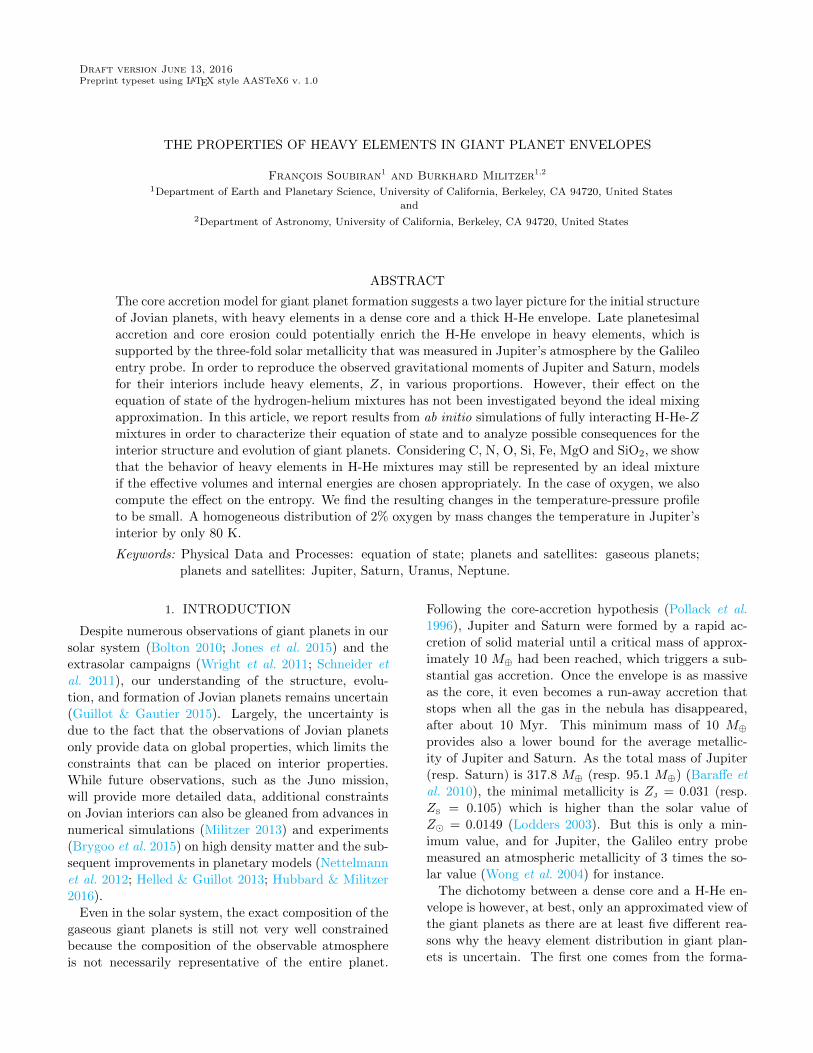
Figure 3. Volume of the H-He-O simulation cell multipliedby the square root of the pressure – to magnify the differences– as a function of the pressure at 10000 K for different oxygencomposition. The symbols show the numerical results andthe curves represent spline interpolations.

modynamic integrations to obtain the Helmholtz free

energy and the entropy. We progressively switched the

interactions in the system from the potential given by

the DFT UDFT to a classical potential Ucl. This methods

has been applied on many systems (de Wijs et al. 1998;

Morales et al. 2009; Wilson & Militzer 2010, 2012a,b;

McMahon et al. 2012; Wahl et al. 2013, 2015). It pro-

vides the Helmotz free energy difference between the two

systems:

FDFT − Fcl =

∫ 1

0

dλ 〈UDFT − Ucl〉λ, (1)

where the parameter λ defines the hybrid potential Uλ =

Ucl +λ(UDFT−Ucl) and the average refers to an average

over configurations computed with the potential Uλ. For

the classical potential, we used a set of non-bonding pair

potentials fitted on the DFT forces. More details of the

integration are given in Soubiran & Militzer (2015a) and

in Wahl et al. (2015).

In order to determine the different thermodynamic

quantities as a function of the pressure rather than the

density, we used a spline interpolation method. For the

pressure and the volume, we used the logarithmic val-

ues as variables for the interpolation. Fig. 3 shows an

example of an interpolation.

3. RESULTS

We investigated the properties of ternary mixtures

with H-He and seven different heavy elements: C, N,

O, Si, Fe, MgO, SiO2. We explored the thermodynamic

properties on two different domains: from 10 to 150

GPa and 2000 to 5000 K, and from 80 to 1500 GPa

and 5000 to 15000 K – see Fig. 2. The thermodynamic

data are presented in Tabs. 3 and 4. We also added the

numerical values of the effective properties we computed

in Tab. 5. For each simulation we computed a one-σ er-

rorbar for the thermodynamic data, based on a block

averaging method (Rapaport 2004). We used standard

error propagation methods for the effective properties.

3.1. Effective volume

For each heavy element, we performed MD-DFT

simulations for 3 different concentrations, keeping

the number of hydrogen and helium atoms constant,

H:He=220:18. We deliberately used a small number of

heavy element atoms – from 2 to 12 – in order to stay in

the diluted limit where the interaction effects between

the heavy species are small. Results for the ternary H-

He-Z mixture were systematically compared with the

binary H-He mixture from Militzer (2013).

In Fig. 3, we plotted the volume-pressure relationship

for different H-He-O mixtures at 10000 K. For a given

pressure, adding oxygen to the mixture results in an in-

crease in the total volume. This effect is magnified in

Fig. 4 where we plotted the volume difference between

the ternary and the binary mixtures as a function of the

number of inserted oxygen atoms. For these conditions,

the volume difference is an almost perfectly linear func-

tion of the number of oxygen atoms. This means that

we can define an effective volume per oxygen atom in

the H-He mixture, at given pressure P and temperature

T , by:

vO,eff =1

NO

[V (NH, NHe, NO)− V (NH, NHe)] , (2)

where V is the volume associated to a mixture of NH

hydrogen, NHe helium and NO oxygen atoms. Recip-

rocally, we can determine the volume for arbitrary but

small concentration in oxygen by using an isothermal-

isobaric additive mixing rule and the aforementioned ef-fective volume of oxygen.

For pressures above 100 GPa and temperatures higher

than 5000 K, we observed a linear behavior of the volume

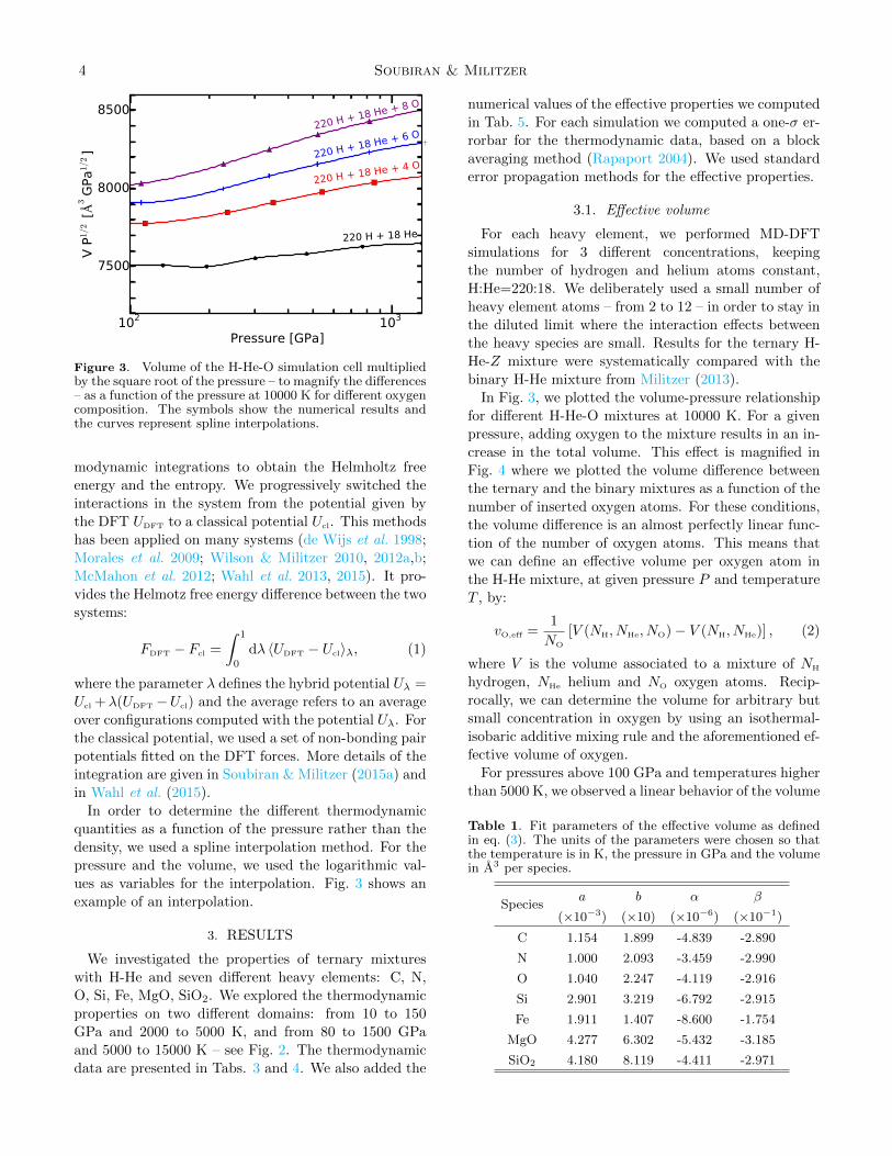
Table 1. Fit parameters of the effective volume as definedin eq. (3). The units of the parameters were chosen so thatthe temperature is in K, the pressure in GPa and the volumein A3 per species.

Speciesa b α β

(×10−3) (×10) (×10−6) (×10−1)

C 1.154 1.899 -4.839 -2.890

N 1.000 2.093 -3.459 -2.990

O 1.040 2.247 -4.119 -2.916

Si 2.901 3.219 -6.792 -2.915

Fe 1.911 1.407 -8.600 -1.754

MgO 4.277 6.302 -5.432 -3.185

SiO2 4.180 8.119 -4.411 -2.971

H-He-Z mixtures 5

0 1 2 3 4 5 6 7 8Number of oxygen atoms

0

10

20

30

40

50

60V

olu

me d

iffe

rence

[3 ]

100 GPa

200 GPa

500 GPa

1000 GPa

1300 GPa

Figure 4. Volume difference between H-He-O and H-Hemixtures as a function of the number of oxygen atoms fordifferent pressures ranging from 100 to 1300 GPa and for atemperature of 10000 K.

difference for each species we considered. In Fig. 5 we

plotted the effective volume of each species that can be

very well fitted as a function of both the temperature

and the pressure with the following simple expression:

veff(P, T ) = (a T + b) PαT+β , (3)

where a, b, α and β are fit parameters given in Tab. (1).

To perform this fit we relied on results ranging from

100 to 1500 GPa, from 5000 to 15000 K and for con-

centrations in heavy elements lower than 5% in number.

We first fitted the effective volume as a power-law of the

pressure, along different isotherms, and using a weighted

least-square fitting procedure. We then fitted the two

coefficients of the power-law as an affine function of the

temperature – of the form a T + b. This provided a ro-

bust fit of the effective volume. This fit is an importantresult of this article because it describes the properties

of heavy species under pressure-temperature conditions

where H-He mixtures are metallic, which makes up for

the major part of giant planet interiors.

We compared the effective volume with the volume of

the pure species as available in the literature. We used

data from ab initio simulations for carbon (Benedict

et al. 2014), nitrogen (Driver & Militzer 2016), oxygen

(Driver et al. 2015), iron and magnesium oxide (Wahl

et al. 2015). Fig. 5 shows a fairly good agreement be-

tween the volume of the pure species and their effec-

tive volume in H-He mixtures for pressure higher than

about 200 GPa. This is not an obvious result as the

interactions are mostly between the heavy species and

hydrogen or helium in the ternary systems while they

are only between the heavy elements themselves in the

pure systems. On the other hand, below 200 GPa, some

deviations have to be noted.

We also compared the effective volume of an SiO2 unit

with the sum of the effective volumes of one silicon and

two oxygen atoms in H-He mixtures. As shown on Fig. 5,

there is a very good agreement between the two esti-

mates, which suggests that, under these conditions, the

system is most likely dissociated. We infer that a similar

behavior is to be expected to any multi-component sys-

tem that would dissociates with increasing temperature

and pressure.

We explored lower pressure-temperature range as well,

from 10 to 150 GPa and 2000 to 5000 K. In some cases

for these conditions, the relationship between the vol-

ume difference and the number of the entities deviates

from a perfect linear relationship. We think that these

deviations may come from the finite duration of our sim-

ulations which may prevent to reach a perfect chemical

equilibrium. We still determined an effective volume

per species through a linear fit and the results are pre-

sented in Fig. 7. To estimate the uncertainty on the

effective volume, we combined the intrinsic statistical

uncertainty of the effective volume with an estimate of

the misfit. For the latter, we computed the effective

volumes, veff,i = ∆V (NZ,i)/NZ,i, from our simulations

with different numbers of heavy species, NZ,i. We then

calculated their standard deviation from the linear fit

value to characterize the misfit. While the statistical

uncertainty is not very sensitive to the temperature or

the pressure, the combined uncertainty of the effective

volumes increases if the temperature decreases, which

can be seen in Fig. 7.

Unlike for the high temperature and pressure condi-

tions, the effective volume of each species does not evolve

monotonically as a function of the pressure in the range

of 10 to 150 GPa and 2000 to 5000 K, and an impor-

tant variability can be observed. It is known that in this

regime, hydrogen undergoes a dissociation and a metal-

lization (Caillabet et al. 2011; Vorberger et al. 2007). By

identifying the nearest neighbors over time as in Soubi-

ran & Militzer (2015a), we determined an estimate of the

dissociation fraction of hydrogen in the H-He mixtures.

In Fig. 7, we see a clear correlation between the drastic

changes of the effective volume of the heavy species and

the dissociation of hydrogen. This result is not surpris-

ing because the interactions between an H2 molecule and

a heavy atom are quite different from the interactions

between an hydrogen ion and the same heavy element.

More specifically, the effective volume increases by

nearly 25% for C, N, O between 60 to 80 GPa at 3000 K,

which could also be linked to chemical reactions with the

surrounding hydrogen. At low temperature and pres-

sure, for instance, carbon tends to form CHx molecules

with x ranging from 0 to 4 (Sherman et al. 2012) and

oxygen associates to hydrogen to form hydroxide or wa-

ter molecules (Soubiran & Militzer 2015b). This chem-

6 Soubiran & Militzer

2

3

4

6

810

15

2025

Volu

me [

Å3 ]

5000 K C

N

O

Si

Iron

MgOSiO2

Si+2O

2

3

4

6

810

15

2025

Volu

me [

Å3 ]

6000 K

2

3

4

6

810

15

2025

Volu

me [

Å3 ]

10000 K

200 400 600 800 1000 1200Pressure [GPa]

2

3

4

6

810

15

20

30

Volu

me [

Å3 ]

15000 K

Computed effective volume

Fitted model

Figure 5. Effective volume for each species in a H-He mix-ture as a function of the pressure for temperatures from 5000to 15000 K. The full curves are the direct results from the vol-ume difference analysis. The light green dash-dotted curveis the sum of the volumes of one Si and two O to be com-pared with the volume of one SiO2. The dashed curves rep-resent the fit based on eq. (3) and the parameters given inTab. (1). The squares (resp. diamonds) represent the vol-ume per species in a pure liquid (resp. solid) phase (Benedictet al. 2014; Driver & Militzer 2016; Driver et al. 2015; Wahlet al. 2015).

istry can also explain the strong deviations of the effec-

tive volume of these species from the volume of the pure

species. It is also interesting to note that iron has a neg-

ative effective volume at the lowest pressure conditions.

We attribute this behavior to a complex chemistry with

hydrogen. In the case of SiO2 we also see a variability in

the effective volume but more importantly, we see that

15

10

5

0

5

10

15

Energ

y [

eV

]

5000 K

C

N

O

Si

Fe

MgO

SiO2

Si+2O

15

10

5

0

5

10

15

20

Energ

y [

eV

]

6000 K

10

5

0

5

10

15

20

Energ

y [

eV

]

10000 K

200 400 600 800 1000 1200Pressure [GPa]

10

5

0

5

10

15

20

25

Energ

y [

eV

]

15000 K

Figure 6. Effective energy for each species in a H-He mix-ture as a function of the pressure for temperatures from 5000to 15000 K. The legend is similar to Fig. 5. At 10000 K, thecolored symbols represent the data for which we forced theenergy to match our data to compensate for any differencein the energy reference.

there are some deviations from the sum of the effective

volumes of one Si and two O atoms. This means that the

system is not dissociated which modifies the interactions

with the H-He mixtures.

The high variability of the effective volume makes it

impossible to give a simple fitting formula but we make

our results on the effective properties available in the

supplementary material attached to this article. Never-

theless, Fig. 7 shows that the formula from eq. (3) with

the parameters from Tab. 1, fitted on the results above

5000 K and 100 GPa, actually well reproduces the lower-

H-He-Z mixtures 7

0

10

20

30

40

50

Volu

me [

Å3 ]

2000 K C

N

O

Si

Iron

MgOSiO2

Si+2O

0

10

20

30

40

50

Volu

me [

Å3 ]

3000 K Computed effective volume

Fitted model

0

10

20

30

40

Volu

me [

Å3 ]

4000 K

25 50 75 100 125Pressure [GPa]

0

10

20

30

40

Volu

me [

Å3 ]

5000 K

0.0 0.1 0.2 0.3 0.4 0.5 0.6 0.7 0.8 0.9 1.0Hydrogen dissociation fraction

Figure 7. Effective volume for each species in a H-He mix-ture as a function of the pressure for temperatures from 2000to 5000 K. The legend is similar to Fig. 5. The colored back-ground represents the dissociation fraction of hydrogen inthe H-He mixture (See Fig. 9 for the actual location of thedissociation in Jupiter). The shaded regions around the Si,MgO and SiO2 curves show the estimated uncertainty.

temperature behavior in the dissociated phase. Namely,

at 5000 K, the fit gives reasonable values starting at

50 GPa, and at 4000 and 3000 K, it gives accurate re-

sults from 80 to 150 GPa.

3.2. Effective internal energy

We investigated the effect of the inclusion of heavy el-

ements in H-He mixtures on the internal energy of the

systems. Since the energy is an extensive thermody-

namic function like the volume, we followed the same

procedure as in the previous section. The energy differ-

25

20

15

10

5

0

5

10

Energ

y [

eV

]

2000 K

C

N

O

Si

Fe

MgO

SiO2

Si + 2 O

20

15

10

5

0

5

Energ

y [

eV

]

3000 K

20

15

10

5

0

Energ

y [

eV

]

4000 K

25 50 75 100 125Pressure [GPa]

20

15

10

5

0

Energ

y [

eV

]

5000 K

0.0 0.1 0.2 0.3 0.4 0.5 0.6 0.7 0.8 0.9 1.0Hydrogen dissociation fraction

Figure 8. Effective energy for each species in a H-He mix-ture as a function of the pressure for temperatures from 2000to 5000 K. The legend is similar to Fig. 7.

ence between the ternary and the binary mixtures ex-

hibits a fairly linear behavior as a function of the number

of heavy element entities (graph not shown). By com-

paring the energy of the ternary mixture of NH hydrogen

atoms, NHe helium atoms and NZ Z entities (atoms or

molecules) with the energy of the binary H-He mixture

at the same pressure P and temperature T , we were able

to determine an effective energy per species Z:

eZ,eff =1

NZ

[E(NH, NHe, NZ)− E(NH, NHe)] . (4)

Our results for the effective energies are plotted in

Fig. 6 and 8. In the dissociated regime, the effective

energy exhibits a fairly smooth evolution with low devi-

8 Soubiran & Militzer

Molecular

Metallic

Core

10000 K ~ 1000 GPa

3500 K ~ 10 GPa5000 K

~ 100 GPa

~ 16000 K ~ 3800 GPa

Figure 9. Schematic view of the interior of Jupiter withthe colors indicating the dissociation of hydrogen as in Figs.7 and 8. We also indicated the order of magnitude of thethermodynamic conditions at different depths.

ations from the linear behavior. We compared the effec-

tive energy with the internal energy of the pure species.

In order to correct for any shift in the origin of the energy

between the different data sources, we artificially made

them to coincide at 10000 K, temperature at which we

had the most data and where we expect every species to

be dissociated. The full symbols in Fig. 6 indicate the

specific data we forced to match the effective energies

we computed. This results in an artificially good match

on the 10000 K isotherm. However, if we look at the

other temperatures, we observe some strong deviations

between the effective energy and the pure species energy,

emphasizing the importance of the inter-species interac-

tions. Below 5000 K, the effective energy exhibits similar

features to the effective volume with drastic variations

as a function of the pressure when hydrogen undergoes

its dissociation.

Overall, we observe that the energy of the ternary

mixtures can be approximated by an isothermal-isobaric

additive mixing rule which is very helpful for evolution

models of planets. However, the effect of the dilution

of the heavy species into the H-He cannot be neglected,

since the effective energy is substantially different from

the internal energy of the pure species.

3.3. Effective entropy

In order to determine the influence of the heavy el-

ements on the temperature-pressure profile of the gi-

ant planets, one needs to compute the entropy of the

ternary mixtures. Hence, we computed the entropy of

ternary mixtures using thermodynamic integrations. As

the computation cost of such calculations is very high,

we only performed it for oxygen in H-He mixtures and

for a subset of temperatures. We shall see in Section 4

250 500 750 1000Pressure [GPa]

5

6

7

8

9

10

11

12

13

14

15

Entr

opy [

kB]

10000 K

5000 K

O effective entropy

H-He entropy

O ideal entropy

H-He ideal entropy

Figure 10. Effective entropy per oxygen atom in a ternaryH-He-O mixtures as a function of the pressure, for 5000 and10000 K. The shaded region represents our estimate of theuncertainty. We also plotted in dashed lines the entropy pernucleus for the binary H-He mixture under the same condi-tions. For comparison, the thin lines show the ideal entropyof pure oxygen and of the H-He mixture under equivalentdensity and temperature conditions.

that it is already enough to determine the effect on the

density profile.

We followed the same procedure as for the volume and

the energy: we computed the entropy of the mixture for

different concentrations and compared the results with

the binary H-He mixture. However, the entropy encom-

passes not only the entropy of each species but also a

mixing entropy. We therefore defined the effective en-

tropy based on the total entropy of the ternary mixtures

of NH hydrogen atoms, NHe helium atoms and NO oxy-

gen atoms and the entropy of the H-He binary mixture,

at constant pressure P and temperature T , by:

sO,eff =1

NO

[S(NH, NHe, NO)− S(NH, NHe)

−∆Smix(NH, NHe, NO)], (5)

where the entropy of mixing is given by:

∆Smix(NH, NHe, NO) =kB ln(NH +NHe +NO)!

−kB ln(NH +NHe)!

−kB lnNO!. (6)

We chose this formula with the explicit factorial term

because the usual Sterling approximation is not appro-

priate for small numbers.

We plotted the effective entropy of oxygen in Fig. 10.

The uncertainty is slightly higher than on the energy

or the volume because the entropy calculation requires

more computation steps but it remains very reasonable

overall, as the maximum uncertainty does not exceed

6 %. We also plotted the entropy per nucleus of the

binary H-He mixtures under the same conditions. For

H-He-Z mixtures 9

comparison we computed the ideal entropy of the H-He

mixture and of oxygen using the Sackur-Tetrode formula

(Reichl 1998):

Sid = kB

∑α

xα

(ln

[vα

(mαkBT

2π~2

)3/2]

+5

2

), (7)

where xα, vα and mα are the concentration ratio, vol-

ume per particle and mass per particle of the particles

of type α respectively. We used the P -V relationship of

the H-He mixture to derive the ideal entropy of H-He

as a function of the pressure. For oxygen, we based our

calculation on the effective volume as derived in section

3.1.

The effective entropy of oxygen is higher than the en-

tropy of H-He, which is simply a mass effect, which is

present in the ideal entropy. Both the effective entropy

of oxygen and entropy of H-He are smoothly decreasing

as pressure increases because the volume per nucleus de-

creases. The non-ideal effects – the difference between

actual and ideal entropy – increase with pressure be-

cause the interactions introduce some local order. The

entropy and effective entropy increase as temperature

increases consistently with the ideal entropy although

the increase is lower for the ideal entropy. We also note

that as the temperature increases, the non-ideal effects

decreases, which is consistent with a diminution of the

interactions effects. We observe that the non-ideal ef-

fects appear more pronounced on the oxygen than on

the H-He mixture. But we have to stress that this is

here only an effective entropy of a single oxygen atom in

a H-He fluid and that the entropy of pure oxygen under

similar conditions may be quite different. The interac-

tions with hydrogen and helium may also influence the

local ordering around the oxygen atoms modifying the

entropy. Last, we want to stress that the variations in

entropy or effective entropy as a function of the pres-

sure and the temperature are quite similar for H-He and

for oxygen, which is important when determining the

internal profile of a giant planet.

4. DISCUSSION

The analysis of the ab initio simulations of several

ternary mixtures showed that, in the diluted regime,

the addition of heavy elements to an H-He mixtures can

be very well described by an ideal isothermal-isobaric

additive mixing rule as long as we employ the effective

properties of the heavy materials as presented in the

previous section. For the higher pressures in the disso-

ciated regime, the effective volume coincides with the

volume of the pure systems but deviations are observed

for lower pressures emphasizing the need for these effec-

tive properties.

In the diluted limit, we can also expect that we can

approximate the properties of a multi-component sys-

tem by simply adding the effective volumes or ener-

gies of each component separately, because the cross-

interactions between different heavy elements should be

negligible compared to the interactions with hydrogen

and helium. This is further supported by the good agree-

ment between the SiO2 effective properties and those of

silicon and oxygen taken separately. This approxima-

tion is however only accurate for the dissociated regime,

which actually represent a significant mass fraction of

the interiors of Jupiter and Saturn. All the previous cal-

culations were performed for a fixed hydrogen to helium

ratio, but the deviations from the pure species properties

are small enough to let us believe that the deviations on

the effective properties, induced by a reasonable change

in helium concentration, should be mostly negligible.

Using the results of our calculations, we studied the

consequences of adding heavy elements in the hydro-

gen and helium rich envelope of giant planets. As a

toy model, we considered as a starting point an homo-

geneous fully convective H-He envelope with a compo-

sition of H:He=220:18 as employed in our simulations.

We picked the temperature at 1 bar to be T = 165 K,

which is close to the Jupiter measured value of 166.1 K

(Seiff et al. 1998), for instance. With this condition and

using Militzer (2013) and Saumon et al. (1995) EOSs, we

were able to determine the pressure-temperature profile,

plotted in Fig. 12. We also computed the density along

the isentrope ρH-He(P ).

With the effective volumes in Tab. (1), we computed

the excess density induced by the addition of a Z =

0.02 mass fraction of different heavy elements homoge-

neously throughout the H-He envelope. The pressure-

temperature profile was kept constant as in Hubbard &

Militzer (2016), and we only perturbed the density.

In Fig. 11, we displayed the relative density difference

between the enriched envelope and the original H-He en-

velope [ρH-He-Z(P )− ρH-He(P )]/ρH-He(P ). The curves are

all for the same mass fraction, Z = 0.02, but for differ-

ent materials. They illustrate by how much the multi-

component mixture deviates from the H-He mixture. In

the most extreme case, when heavy atoms have a negli-

gible volume, a 2% mass fraction leads to a 2% density

change. As expected, the densest species – iron and

silicon dioxide – introduce the largest density change,

close to a 2% density increase for a 2% mass fraction.

On the other hand, the inclusion of Synthetic Uranus

(SU) induces a 1% density increase only. SU is a proxy

that we used to mimic a mixture of ice derivatives based

on oxygen, nitrogen, carbon and hydrogen in a ratio of

H:O:C:N=87:25:13:4. It was first introduced as a proxy

for Uranus interior in high pressure laboratory experi-

ments (Nellis et al. 1997), and it was also used in the

recent Jupiter model by Hubbard & Militzer (2016) to

enrich the envelope. The relatively low density of SU

10 Soubiran & Militzer

0 500 1000 1500 2000Pressure [GPa]

1.0

1.2

1.4

1.6

1.8

2.0R

ela

tive d

ensi

ty d

iffe

rence

[%

]

IronSiO2

Oxygen

Synthetic Uranus

Figure 11. Relative density difference, along the H-He isen-trope of a giant planet with T = 165 K at 1 bar, between asimple H-He mixture and a multi-component mixture includ-ing a 2 % mass fraction of heavy elements. Synthetic Uranusrefers to a mixture of ice derivatives as presented in Nellis etal. (1997); Hubbard & Militzer (2016). For this species, wechose a composition of H:O:C:N=87:25:13:4.

is due to the presence of a high amount of hydrogen

that we chose to include in the computation of the Z

fraction. For comparison, oxygen has a slightly higher

density with a density increase of roughly 1.5%.

We showed that the addition of heavy elements in the

H-He mixture slightly influenced the density of the mix-

ture. It is thus natural to infer that they may have an in-

fluence on the entropy as well, and thus, on the pressure-

temperature profile of the envelope. Yet, a change in

the P -T relationship in the planet would also change its

density profile and it has to be accounted for. Besides

the case of the unperturbed H-He isentrope in Fig. 12,

we explored three different scenarios for the enriched

layer. The first scenario is a single layer of a H-He-O

mixture with a Z = 0.02 mass fraction in oxygen but

this time taking the entropy change into account. We

then explored two other scenarios with a two-layer pic-

ture where the outer layer is made of H-He solely and

the inner layer is an enriched H-He mixture with 2% of

oxygen. The difference lies in the temperature at the

interface between the two layers: in one case we consid-

ered a 3500 K interface, in the other we picked 5000 K.

The resulting properties for the different scenarios are

summarized in Tab. (2).

For the first scenario, we assumed that the oxygen

reacted with the surrounding hydrogen at 165 K and

1 bar to form water molecules. We further assumed that

water is in a vapor state as the concentration is low. We

then could compute the entropy of the mixture at 165 K

and 1 bar by:

s=xH2sH2

+ xHesHe + xH2OsH2O

−kB(xH2lnxH2

+ xHe lnxHe + xH2O lnxH2O), (8)

where xα (resp. sα) is the number fraction (resp. en-

tropy per molecule) of molecules of type α. We used

Saumon et al. (1995) EOS to compute the entropy of H

and He. For water, we used the entropy from the trans-

lational, rotational and vibrational degrees of freedom

as in Vidler & Tennyson (2000).We obtained an entropy

of 7.607 kB/nucleus for the whole mixture.

Following a constant entropy line, and using the ef-

fective entropy of oxygen computed in Section 3.3, we

were able to compute theP -T relationship above 4000 K

and 10 GPa, as represented in Fig. 12. The comparison

with the unperturbed isentrope shows that the oxygen

entropic effects result in an increase of the pressure by

3% for a given temperature. Equivalently, it results in a

temperature decrease of roughly 80 K at constant pres-

sure. The effect on the density can be seen in Fig. 13:

compared to the original H-He profile, the density varia-

tion induced by the oxygen increases from 1.5% without

the entropy correction to 1.6% when taking the entropy

of oxygen into account. Since this is a rather marginal

effect, it is hard to believe that this difference could be

resolved by Juno measurements of the gravitational mo-

ments. We find it reasonable to use the original H-He

isentrope for giant planet modeling (Hubbard & Militzer

2016).

The second and third scenarios are based on a two-

layer picture with a pure H-He outer envelope and an

inner envelope with a 2% mass fraction of oxygen. The

outer layer has the unperturbed P -T profile and the en-

riched inner layer profile is determined by the condi-

tion at the interface: we computed the entropy of the

ternary H-He-O mixture assuming that, at the inter-

face, the pressure and the temperature were the same

in both layers. The resulting profiles are represented by

the symbols in Figs. 12 and 13. If we let the inner layer

start in the molecular phase, at 3500 K and 7.2 GPa,

we retrieve to a very good accuracy the predictions of

the single layer. It is mostly the dissociation that drives

the slight shift in the isentrope and it occurs at tem-

peratures higher than 3500 K. On the other hand, if we

Table 2. Properties of the hypothetical isentropes in an H-He envelope enriched with 2% oxygen in mass and with a165 K temperature at 1 bar. The first two models are for asingle layer without or with entropy correction. The last twomodels are for a two-layer picture with the enriched layeronly for temperatures higher than 3500 or 5000 K. For eachhypothesis, we give the entropy per nucleus S as well as thepressures at 5000 and 10000 K.

DescriptionS P5000K P10000K

(kB/nucl.) (GPa) (GPa)

Unperturbed H-He 7.598 95.6 927

H-He-O mono-layer 7.607 98.6 950

H-He-O starts at 3500 K 7.605 98.9 953

H-He-O starts at 5000 K 7.624 95.6 929

H-He-Z mixtures 11

4000

6000

8000

10000

12000

14000Tem

pera

ture

[K

] H-He isentrope

H-He with water vapor at 165K

H-He-O starting at 3500K

H-He-O starting at 5000K

900 950 100098009900

100001010010200

90 100 110

4950500050505100

0 500 1000 1500 2000Pressure [GPa]

100

50

0

∆ T

[K

]

Figure 12. Pressure-temperature profile in the H-He enve-lope of a gaseous planet with T = 165 K at 1 bar with a 2%mass fraction of oxygen. The full and dashed lines are fora single layer of H-He-O with or without entropy correctiondue to the presence of oxygen. The discrete symbols are for atwo-layer picture, where the 2% oxygen enriched layer startsat 3500 or 5000 K. A summary of the properties of theseprofiles can be found in Tab. (2). The bottom graph showsthe temperature difference between the different profiles withthe original H-He profile.

let the inner layer start at 5000 K and 95.6 GPa, in the

dissociated phase, the predicted isentrope is almost ex-

actly the same as the H-He isentrope. The temperature

difference is lower than 10 K at a given pressure and

the pressure is increased by only 0.2% at 10000 K (see

Tab. (2)). The entropy itself is modified by the pres-

ence of oxygen, but this shift is nearly constant along

the H-He isentrope in the dissociated phase, which ex-

plains the absence of impact on the predicted pressure-

temperature profile and thus on the density. We expect

this observation to be true for the other heavy element

as well, especially in the diluted limit.

The last scenario with the temperature at the interface

at 5000 K is of interest for cold giant planet modeling.

When the planet is cold enough, a phase separation of

hydrogen and helium is indeed expected to occur, natu-

rally differentiating the envelope in (at least) two layers.

The innermost layer and helium enriched is entirely in

the dissociated regime (Guillot 2005; Hubbard & Mil-

itzer 2016) and is also the one the most subject to heavy

element enrichment because in direct contact with the

eroding core. Yet, we showed on the example of oxygen

that in this regime, the entropy of the heavy element

play virtually no role on the pressure-temperature pro-

file that can thus be determined by the H-He properties

solely. This means that to model this innermost layer,

the H-He EOS and the effective volumes of the heavy

elements are sufficient to properly recover the density

profile.

5. MASS-RADIUS RELATIONSHIP

0 500 1000 1500 2000Pressure [GPa]

1.4

1.5

1.6

1.7

1.8

1.9

Rela

tive d

ensi

ty d

iffe

rence

[%

] H-He-O one-layerwithout entropy correction

H-He-O one-layerwith entropy correction

H-He-O starting at 3500K

H-He-O starting at 5000K

Figure 13. Relative density difference between a simple H-He mixture and a multi-component mixture including a 2%mass fraction of oxygen along the P -T profile of the envelopeof a giant planet with a 165 K temperature at 1 bar. Thedashed blue (resp. solid red) curve shows the density increasefor a single layer without (resp. with) the entropy correctiondue to the oxygen. The green circles (resp. cyan squares)are for a two-layer hypothesis with an outer H-He layer andan inner H-He-O layer starting at 3500 K (resp. 5000 K).The corresponding P -T profiles are those of Fig. 12.

In this section, we briefly discuss the effects that heavy

elements have on the mass-radius relationship of gas gi-

ant exoplanets. To simplify our analysis, we only con-

sider planets without a rocky core and assume a homo-

geneous, convective interior. The adiabatic P -T profile

is derived from a H-He mixture starting from 1 bar and

166.1 K. For a given planet mass, the radius is derived by

solving the ordinary differential equations of the hydro-

static equilibrium (Seager et al. 2007; Wilson & Militzer

2014). Fig. 14 shows the effect that the introduction of a

2% and a 4% mass fraction of oxygen has on the radius

of a giant planet. We find that a Jupiter-mass planetrespectively shrinks by 0.7% and 2.4% in radius. Ac-

cording to eq. (3), the introduction of oxygen not only

increases the mass but also the volume of the H-He mix-

ture at given pressure and temperature. As a result, the

density increases by less than 2% or 4%; respectively.

In order to disentangle both effects, we plot the mass-

radius relationship for planets where we have increased

the H-He density by 2% and 4% in Fig. 14. We find that

a Jupiter-mass planet then shrinks by 1.7% and 3.3% in

radius; respectively.

It is interesting to note that the effect of heavy ele-

ments is much larger if one compares different planet

masses for a given radius. Since giant planets have de-

generate interiors, their radii start to shrink if a mass of

approximately 3 Jupiter masses is exceeded. Jupiter’s

radius is not too different from the maximum radius of

approximately 1.2 RJ (Seager et al. 2007). The slope of

the mass-radius curves in Fig. 14 is thus relatively small

12 Soubiran & Militzer

0.0 0.2 0.4 0.6 0.8 1.0 1.2Planet mass (MJ )

0.90

0.95

1.00

1.05Pla

net

radiu

s (R

J)

Original H-He planet

H-He + 2% oxygen

H-He + 2% density increase

H-He + 4% oxygen

H-He + 4% density increase

Figure 14. Mass-radius relationship in Jupiter units for gi-ant planets without a rocky core. The adiabatic interiorP -ρ-T profiles are derived from H-He mixture with an effec-tive temperature of 166.1 K at 1 bar. The thin solid lineshows the radii of the H-He planets without heavy elements.The thin dashed lines illustrate the effect that a 2% or 4%increase in density has on the planet radius. The thick linesshow the effect of introducing a 2% and 4% mass fraction ofoxygen.

and a modest change in radius has a significant effect

on the inferred planet mass. For a fixed radius of 1 RJ,

the mass of a core-less planet increases from 0.63 to 0.70

or 0.86 MJ if an oxygen mass fraction of 2% or 4% is

introduced; respectively.

6. CONCLUSIONS

Ab initio simulations showed that, in the diluted

limit, ternary mixtures made of hydrogen and helium

in roughly solar abundance with heavy elements can be

very well approximated by an isothermal-isobaric ad-

ditive mixing rule on the volume and the energy un-

der thermodynamic conditions relevant in the interior

of giant planets. It is however necessary to use effective

volume and energy for the heavy elements because the

dominant contributions come from the cross-interactions

with hydrogen and helium. Although these effective

properties tend towards the pure species volume and en-

ergy at high pressure and temperature, there are signif-

icant discrepancies at lower pressure and temperature.

The study of the entropy of oxygen showed that in the

diluted limit, the effective entropy is mostly influenced

by the dissociation of hydrogen but stays rather constant

along the H-He isentrope in the dissociated regime. If

we consider a H-He giant planet with a 2% oxygen mass

fraction, the net increase in density is of about 1.5%

compared to a pure H-He envelope, for given pressure

and temperature. Including the entropy correction, the

addition of 2% oxygen increases the pressure by roughly

3% at a given temperature or, equivalently, decreases

the temperature by less than 2% at a given pressure.

The effect of the entropy is thus very small and the net

over-density is only of the order of 0.1%.

In the case of a two-layer model with an upper layer

made of H-He and an oxygen enriched inner layer en-

tirely in the metallic regime, the predicted pressure-

temperature profile do not deviate from the pure H-He

predictions. Overall, in the diluted limit, the entropy

appears to have very little effect on the density-pressure

relationship.

We argue that the use of the isentrope properties of

the H-He mixture with the effective volume and energy

of the heavy elements as described in this article should

give a very good approximation of the actual profile of

giant planets. The comparison with the coming data on

the gravitational moments should help to constrain the

distribution of heavy elements in these planets.

ACKNOWLEDGMENTS

This work was supported by NASA and NSF. Com-

puters at NAS, XSEDE and NCCS were used.

REFERENCES

Baldereschi, A. 1973, PhRvB, 7, 5212.

Baraffe, I., Chabrier, G. & Barman, T. 2008, A&A 482, 315.

Baraffe, I., Chabrier, G. & Barman, T. 2010, RPPh 73, 016901.

Benedict, L. X., Driver, K. P., Hamel, S., Militzer, B., Qi, T.,

Correa A. A., Saul, A. & Schwegler, E. 2014, PhRvB, 89,

224109.

Blochl, P. E. 1994, PhRvB, 50, 17953.

Bolton, S. J. 2010. The Juno Mission. Proceedings of the

International Astronomical Union, 6, pp 92-100.

Brygoo, S., Millot, M., Loubeyre, P., Lazicki, A. E., Hamel, S.,

Qi, T., Celleirs, P. M., Coppari, F., Eggert, J. H.,

Fratanduono, D. E., Hicks, D. G., Rygg, J. R., Smith, R. F.,

Swift, D. C., Collins, G. W. & Jeanloz, R. 2015, JAP, 118,

195901.

Caillabet, L., Mazevet, S. & Loubeyre, P. 2011, PhRvB, 83,

094101.

Denœud, A., Benuzzi-Mounaix, A., Ravasio, A., Dorchies, F.,

Leguay, P. M., Gaudin, J., Guyot, F., Brambrink, E., Koenig,

M., Le Pape, S. & Mazevet, S. 2014, PhRvL, 113, 116404.

Driver, K. P., Soubiran, F., Zhang, S. & Militzer, B. 2015,

JChPh, 143, 164507.

Driver, K. P. & Militzer, B. 2016, PhRvB, 93, 064101.

Fortney, J. J. & Hubbard, W. B. 2004, ApJ, 608, 1039.

Fortney, J. J., Mordasini, C., Nettelmann, N., Kempton,

E. M.-R., Greene, T. P. & Zahnle, K. 2013, ApJ, 775, 80.

Fuller, J., Lai, D. & Storch, N. I. 2014, Icar, 231, 34.

Fuller, J. 2014, Icar, 242, 283.

Gaulme, P., Schmider, F.-X., Gay, J., Guillot, T. & Jacob, C.

2011, A&A, 531, A104.

H-He-Z mixtures 13

Gonzalez-Cataldo, F., Wilson, H. F. & Militzer, B. 2014, ApJ,

787, 79.

Guillot, T. 2005, AREPS, 33, 493.

Guillot, T. & Gautier, D. 2015. Giant Planets. In: Schubert, G.

(Ed.), Treatise on Geophysics (2nd Edition). Elsevier, Oxford,

pp. 529 - 557.

Helled, R. & Guillot, T. 2013, ApJ, 767, 113.

Hohenberg, P. & Kohn, W. 1964, PhRv, 136, 864.

Hubbard, W. B. & Militzer, B. 2016, ApJ, 820, 13.

Jones, D. L., Folkner, W. M., Jacobson, R. A., Jacobs, C. S.,

Dhawan, V., Romney, J. & Fomalont, E. 2015, AJ, 149, 28.

Kohn, W. & Sham, L. J. 1965, PhRv, 140, 1133.

Kresse, G. & Furthmuller, J. 1996, PhRvB, 54, 11169.

Leconte, J. & Chabrier, G.2012, A&A 540, A20.

Leconte, J. & Chabrier, G.2013, NatGe 6, 347.

Lodders, K. 2003, ApJ, 591, 1220.

Lorenzen, W., Holst, B. & Redmer, R. 2009, PhRvL, 102,

115701.

Lorenzen, W., Holst, B. & Redmer, R. 2011, PhRvB, 84, 235109.

McMahon, J. M., Morales, M. A., Pierleoni, C. & Ceperley,

D. M. 2012, RvMP, 84, 1607.

Mermin, N. D. 1965, PhRv, 137, A1441.

Militzer, B. 2009, PhRvB, 79, 155105.

Militzer, B. 2013, PhRvB, 87, 014202.

Militzer, B. & Hubbard, W. B. 2013, ApJ, 774, 148.

Militzer, B. & Driver, K. P. 2015, PhRvL, 115, 176403.

Morales, M. A., Pierleoni, C., Schwegler, E. & Ceperley, D. M.

2009, PNAS, 106, 1324.

Morales, M. A., Hamel, S., Caspersen, K. & Schwegler, E. 2013,

PhRvB, 87, 174105.

Nellis, W., Holmes, N., Mitchell, A., Hamilton, D., & Nicol, M.

1997, JChPh, 107, 9096.

Nettelmann, N., Becker, A., Holst, B. & Redmer, R. 2012, ApJ,

750, 52.

Nettelmann, N., Helled, R., Fortney, J. &Redmer, R. 2013,

P&SS, 77, 143.

Nose, S. 1984, JChPh, 81, 511.

Nose, S. 1991, PThPS, 103, 1.

Perdew, J. P., Burke, K. & Ernzerhof, M. 1996, PhRvL, 77, 3865.

Pollack, J. B., Hubickyj, O., Bodenheimer, P., Lissauer, J. J.,

Podolak, M. & Greenzweig, Y. 1996, Icar, 142, 62.Rapaport, D. C. 2004, The Art of Molecular Dynamics

Simulation, Cambridge University Press.

Reichl, L. E. 1998, A modern course in statistical physics, 2nded., Wiley-Interscience

Saumon, D., Chabrier, G. & van Horn, H. M. 1995, ApJSS, 99,

713.Schneider, J., Dedieu, C., Sidaner (Le), P., Savalle, R. &

Zolotukhin, I. 2011, A&A, 532, A79.

Seager, S., Kuchner, M., Hier-Majumder, C. A. & Militzer, B.2007, ApJ, 669, 1279.

Seiff, A., Kirk, D. B., Knight, T. C. D., Young, R. E., Mihalov,J. D., Young, L. A., Milos, F. S., Schubert, G., Blanchard,

R. C. & Atkinson 1998, JGR, 103, 22857.

Sherman, B. L., Wilson, H. F., Weerartane, D. & Militzer, B.2012, PhRvB, 86, 224113.

Soubiran, F., Mazevet, S., Winisdoerffer, C. & Chabrier, G.

2013, PhRvB, 87, 165114.Soubiran, F. & Militzer, B. 2015, ApJ, 806, 228.

Soubiran, F. & Militzer, B. 2015, HEDP, 17, 157.

Stevenson, D. J. & Salpeter, E. E. 1977, ApJS, 35, 239.Stevenson, D. J. 1982, P&SS, 30, 775.

Vidler, M. & Tennyson, J. 2000, JChPh, 113, 21.

Vorberger, J., Tamblyn, I., Militzer, B. & Bonev, S. A. 2007,PhRvB, 75, 024206.

Wahl, S. M., Wilson, H. F. & Militzer, B. 2013, ApJ, 773, 95.Wahl, S. M., Wilson, H. F. & Militzer, B. 2015, E&PSL, 410, 25.

de Wijs, G. A., Kresse, G. & Gillan, M. J. 1998, PhRvB, 57, 8223Wilson, H. F. & Militzer, B. 2010, PhRvL, 104, 121101.

Wilson, H. F. & Militzer, B. 2012, ApJ, 745, 54.

Wilson, H. F. & Militzer, B. 2012, PhRvL, 108, 111101.Wilson, H. F. & Militzer, B. 2014, ApJ, 973, 34.

Wong, M. H., Mahaffy, P. R., Atreya, S. K., Niemann, H. B. &

Owen, T. C. 2004, Icar, 171, 153.Wright, J. T., Fakhouri, O., Marcy, G. W., Han, E., Feng, Y.,

Johnson, J. A., Howard, A. W., Fischer, D. A., Valenti, J. A.,

Anderson, J. & Pisnukov, N. 2011, PASP, 123, 412.

14 Soubiran & Militzer

Table 3. Pressure and internal energy of H-He-Z mixtures with 220 H, 18 He and NZ

heavy entities.

SpeciesTemperature

NZVolume Pressure Internal Energy

(K) (A3/nucl.) (GPa) (eV/nucl.)

C 2000 4 3.88922 42.131±0.040 -2.48961±0.00099

C 2000 4 3.21772 65.040±0.136 -2.30810±0.00149

C 2000 4 2.72109 95.333±0.153 -2.09755±0.00139

C 2000 4 2.36276 127.530±0.345 -1.84461±0.00370

C 2000 6 6.23309 14.638±0.075 -2.81747±0.00184

C 2000 6 4.74436 27.363±0.082 -2.68190±0.00144

Note—Table 3 is published in its entirety in the electronic edition of the AstrophysicalJournal. A portion is shown here for guidance regarding its form and content.

Table 4. Pressure and internal energy of H-He-O mixtures with 220 H, 18 He and NO O atoms.

TemperatureNO

Volume Pressure Internal Energy Helmholtz Free Energy

(K) (A3/nucl.) (GPa) (eV/nucl.) (eV/nucl.)

5000 4 2.27838 157.151±0.133 -1.07385±0.00128 -4.26949±0.00067

5000 4 1.67448 317.938±0.131 -0.43909±0.00139 -3.42557±0.00043

5000 4 1.18800 684.367±0.170 0.73063±0.00165 -2.00307±0.00031

5000 6 3.19134 75.024±0.123 -1.52485±0.00218 -4.92724±0.00077

5000 6 2.69878 109.354±0.115 -1.33611±0.00202 -4.64932±0.00075

5000 6 2.25970 164.723±0.129 -1.07571±0.00102 -4.28233±0.00057

Note—Table 4 is published in its entirety in the electronic edition of the Astrophysical Journal. Aportion is shown here for guidance regarding its form and content.

Table 5. Effective properties of heavy elements in H-He mixtures.

SpeciesTemperature Pressure Volume Internal Energy Entropy

(K) (GPa) (A3) (eV) (kB)

O 5000 1050 3.018±0.063 0.196±0.718 8.51±0.56

O 5000 1100 2.937±0.072 0.281±0.798 8.53±0.61

O 5000 1150 2.859±0.081 0.353±0.879 8.55±0.68

O 5000 1200 2.784±0.090 0.413±0.962 8.57±0.75

O 6000 100 6.377±0.082 5.136±0.210

O 6000 150 5.853±0.061 4.740±0.237

Note—The effective entropy is only available for oxygen and only at 5000 and 10000 K.Table 5 is published in its entirety in the electronic edition of the Astrophysical Journal.A portion is shown here for guidance regarding its form and content.