Frank Germann, Peter Ebbes, & Rajdeep Grewal The …moorman/Marketing-Strategy-Seminar... · Frank Germann, Peter Ebbes, & Rajdeep Grewal The Chief Marketing Officer Matters! Marketing

Frank Germann, Peter Ebbes, & Rajdeep Grewal

The Chief Marketing Officer Matters!Marketing academics and practitioners alike remain unconvinced about the chief marketing officer’s (CMO’s)performance implications. Whereas some studies propose that firms benefit financially from having a CMO in theC-suite, other studies conclude that the CMO has little or no effect on firm performance. Accordingly, there have beenstrong calls for additional academic research regarding the CMO’s performance implications. In response to thesecalls, the authors employ model specifications with varying identifying assumptions (i.e., rich data models, unobservedeffects models, instrumental variable models, and panel internal instruments models) and use data from up to 155publicly traded firms over a 12-year period (2000–2011) to find that firms can indeed expect to benefit financially fromhaving a CMO at the strategy table. Specifically, their findings suggest that the performance (measured in terms ofTobin’s q) of the sample firms that employ a CMO is, on average, approximately 15% greater than that of the samplefirms that do not employ a CMO. This result is robust to the type of model specification used. Marketing academics andpractitioners should find the results intriguing given the existing uncertainty surrounding the CMO’s performanceimplications. The study also contributes to the methodology literature by collating diverse empirical model specificationsthat can be used to model causal effects with observational data into a coherent and comprehensive framework.

Keywords: chief marketing officer performance implications, marketing–finance interface, panel data, endogeneity,instrumental variable

Online Supplement: http://dx.doi.org/10.1509/jm.14.0244

Frank Germann is Assistant Professor of Marketing, Mendoza College ofBusiness, University of Notre Dame (e-mail: [email protected]). PeterEbbes is Associate Professor of Marketing, HEC Paris (e-mail: ebbes@hec. fr). Rajdeep Grewal is the Townsend Family Distinguished Professorof Marketing, Kenan-Flagler Business School, University of North Caro-lina at Chapel Hill (e-mail: [email protected]). The authors thank ChelseaDeBoer, Manisha Goswami, Lauren Harville, Bernard O’Neill, and Kim-berly Sammons for their research assistance and Shrihari Sridhar andSriram Venkataraman for their helpful feedback on an earlier version ofthe article. In addition, they gratefully acknowledge the constructive guid-ance of the JM review team. Peter Ebbes acknowledges research supportfrom Investissements d’Avenir (ANR-11-IDEX-0003/LabexEcodec/ANR-11-LABX-0047). Christine Moorman served as area editor for this article.

© 2015, American Marketing AssociationISSN: 0022-2429 (print), 1547-7185 (electronic)

Journal of MarketingVol. 79 (May 2015), 1 –221

In 2008, Nath and Mahajan reported that “[Chief market-ing officer] presence in the Top Management Team(TMT) has neither a positive nor a negative impact on

firm performance” (p. 65). In the words of Barta (2011),this finding “has caused quite a stir [among marketers]”because “firms with a CMO on the management team arenot more successful than firms without a CMO.” Moreover,Frazier (2007, p. 3)1 urged CMOs to “hide this publication”because they are being “rapped for having zero impact.” Inshort, Nath and Mahajan’s (2008; hereinafter N&M) (lackof) findings have made many marketers nervous (also seeShoebridge 2007; Simms 2008). Yet their work has raisedan important question: Do CMOs matter?

There is some evidence that suggests that CMOs shouldpositively influence firm performance. For example, usingdata from 1987–1991 (in contrast, N&M use 2000–2004

data), Weinzimmer et al. (2003) find a positive correlationbetween CMO presence and sales growth. It is also widelybelieved that CMO presence raises the importance of mar-keting in the C-suite, which in turn should bring the cus-tomer to the boardroom and thereby improve firm perfor-mance (e.g., Kerin 2005; McGovern et al. 2004). Moreover,using an event study of CMO announcements, Boyd,Chandy, and Cunha (2010) find that the impact of CMOs onfirm performance is contingent on the managerial discretionavailable to them. In addition, using the same sample as intheir 2008 study, Nath and Mahajan (2011) report that pow-erful CMOs have a positive impact on sales growth.

However, researchers still seem unconvinced about theCMO’s performance implications, as evidenced by theirstrong calls for additional research. For example, Boyd,Chandy, and Cunha (2010, p. 1174) assert that “the CMOremains a rather enigmatic creature in academic literature”and “the scarcity of … research … is lamentable.” Simi-larly, Nath and Mahajan (2011, p. 74) urge for additionalresearch to “shed further light on the issue of CMO pres-ence.” Moreover, in summarizing the findings from a recentCMO survey, Moorman (2013) reports that demonstratingthe value of marketing remains a general challenge forCMOs. Indeed, approximately 66% of the CMOs surveyedstate that they are experiencing pressure from their chiefexecutive officer (CEO) or board to prove the value of mar-keting. Moreover, due to their nonfindings regardingCMOs’ performance implications, N&M is still oft-cited inthe media (e.g., Whitler 2013).

Against this backdrop, we build on N&M’s work andseek a more comprehensive examination than what is avail-able in the literature to model the causal effect of CMO

1It seems that Frazier (2007) had access to the prepublicationversion of Nath and Mahajan (2008).

presence on firm performance. Specifically, using N&M’sresearch as a starting point, we extend their work in threeimportant directions:

1. Time horizon: N&M included five years of data in theirstudy. Considering that executives’ performance effectstake time to manifest (e.g., Hambrick and Fukutomi 1991;Miller and Shamsie 2001), we extend N&M’s sample byseven years (i.e., for a total of 12 years [2000–2011] vs. fiveyears [2000–2004]).

2. Industries. N&M included a wide range of industries intheir data set but excluded certain others (e.g., Food andKindred Products [e.g., General Mills]; TransportationEquipment [e.g., Ford Motor Co.]; Miscellaneous Manufac-turing Industries [e.g., Mattel, Inc.]). We include these addi-tional industries in our analysis.

3. Model. We consider several econometric extensions overN&M. First, N&M employed between-effects regressionand, thus, did not exploit the panel structure of their data.For relatively short time series (five years for N&M), usinga between-effects model might be appropriate; however,because we include considerably more years in some of oursamples, we explicitly exploit the panel structure by includ-ing time and firm effects in our analyses, which corrects forcommon unobserved time shocks and unobserved time-invariant firm-specific factors, respectively. Second, on thebasis of results from a residual test, N&M treated CMO

2 / Journal of Marketing, May 2015

presence as exogenous; however, CMO presence is likelythe result of a strategic firm decision, and treating CMOpresence as an exogenous regressor might result in incon-sistent estimates. We address the potentially endogeneousCMO effect by (a) exploiting the panel structure of the dataand (b) using instrumental variables (IVs).

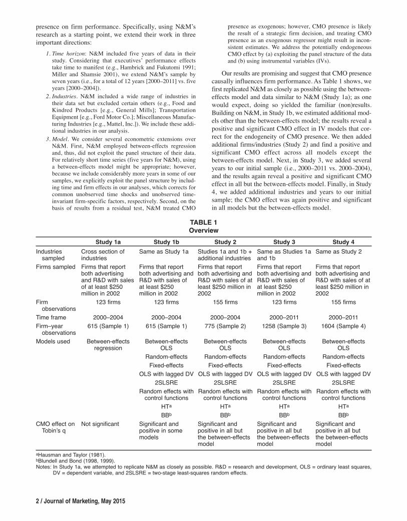
Our results are promising and suggest that CMO presencecausally influences firm performance. As Table 1 shows, wefirst replicated N&M as closely as possible using the between-effects model and data similar to N&M (Study 1a); as onewould expect, doing so yielded the familiar (non)results.Building on N&M, in Study 1b, we estimated additional mod-els other than the between-effects model; the results reveal apositive and significant CMO effect in IV models that cor-rect for the endogeneity of CMO presence. We then addedadditional firms/industries (Study 2) and find a positive andsignificant CMO effect across all models except thebetween-effects model. Next, in Study 3, we added severalyears to our initial sample (i.e., 2000–2011 vs. 2000–2004),and the results again reveal a positive and significant CMOeffect in all but the between-effects model. Finally, in Study4, we added additional industries and years to our initialsample; the CMO effect was again positive and significantin all models but the between-effects model.

Study 1a Study 1b Study 2 Study 3 Study 4Industries sampled

Cross section ofindustries

Same as Study 1a Studies 1a and 1b +additional industries

Same as Studies 1aand 1b

Same as Study 2

Firms sampled Firms that reportboth advertisingand R&D with salesof at least $250 million in 2002

Firms that reportboth advertising andR&D with sales ofat least $250 million in 2002

Firms that reportboth advertising andR&D with sales of atleast $250 million in2002

Firms that reportboth advertising andR&D with sales ofat least $250 million in 2002

Firms that reportboth advertising andR&D with sales of atleast $250 million in2002

Firm observations

123 firms 123 firms 155 firms 123 firms 155 firms

Time frame 2000–2004 2000–2004 2000–2004 2000–2011 2000–2011Firm–yearobservations

615 (Sample 1) 615 (Sample 1) 775 (Sample 2) 1258 (Sample 3) 1604 (Sample 4)

Models used Between-effectsregression

Between-effectsOLS

Random-effectsFixed-effects

OLS with lagged DV2SLSRE

Random effects withcontrol functions

HTaBBb

Between-effectsOLS




HTaBBb

Between-effectsOLS




HTaBBb

Between-effectsOLS




HTaBBb

CMO effect onTobin’s q

Not significant Significant and positive in somemodels

Significant and positive in all but the between-effectsmodel

Significant and positive in all butthe between-effectsmodel

Significant and positive in all but the between-effectsmodel

TABLE 1Overview

aHausman and Taylor (1981).bBlundell and Bond (1998, 1999).Notes: In Study 1a, we attempted to replicate N&M as closely as possible. R&D = research and development, OLS = ordinary least squares,

DV = dependent variable, and 2SLSRE = two-stage least-squares random effects.

Thus, our findings suggest that firms can indeed expectto benefit financially from having a CMO at the strategytable. More specifically, our data and analyses suggest thatfirm performance (i.e., Tobin’s q) for firms with a CMO isapproximately 15% better than that of firms without aCMO. The positive and significant effect of CMO presenceis confirmed when we use excess stock returns (i.e.,Jensen’s a) as an alternate performance metric.

Beyond the substantive insight that CMOs providevalue, our article also makes methodological contributions.Recognizing the nature of our data (i.e., secondary data on alarge number of firms over several years), we identify anddescribe in detail four observational data modelingapproaches that could be adopted to study complex market-ing strategy phenomena such as the CMO’s performanceimplications: (1) rich data models, (2) unobserved effectsmodels, (3) IV models, and (4) panel internal instrumentsmodels. We hope that our discussion will encourage readersto see themselves as regression engineers—that is, under-stand the meaning of the model identifying assumptions—as opposed to “regression mechanics”—that is, estimate alarge number of models and report the best results (Angristand Pischke 2009, p. 28).

In what follows, we first briefly revisit N&M. We thendiscuss our modeling framework, describe our data andsamples, and present our findings. We conclude with a dis-cussion of our findings and the limitations of our research.

BackgroundWe begin by providing the relevant aspects of N&M’s studyand then outline how we build on their research. N&Mexplore two related research questions: (1) What organiza-tional factors are associated with CMO presence in TMTs?(2) Does CMO presence affect firm performance? Theyfind that several firm factors such as the level of innovative-ness (i.e., research and development [R&D] to sales ratio)and differentiation (i.e., advertising to sales ratio) are asso-ciated with the likelihood of CMO presence in the TMT.They also find that CMO presence has no statistical effecton firm performance, neither by itself nor when analyzedjointly with the various firm factors (e.g., interactionsbetween CMO presence and innovativeness). This nonfind-ing regarding the CMO’s performance implications formsthe crux of our research.

Over five years (2000–2004), N&M observed 167 firmsfrom a cross section of industries. They included all firmsfrom the Compustat database with sales of at least $250million in 2002, the midpoint of their observation period.From this set, they retained only firms without missing dataon variables such as advertising and R&D as well as theirtwo dependent variables, Tobin’s q and sales growth. Anexecutive listed in the TMT with the term “marketing” inhis or her title implied CMO presence. As we discuss in our“Samples and Measures” section, we carefully followedN&M’s data collection approach. We note that, in additionto Tobin’s q and sales growth, we assess the CMO’s impacton excess stock return (i.e., Jensen’s a) and firm systematicand idiosyncratic risk.

The Chief Marketing Officer Matters! / 3

Model Specification andIdentification

Our primary objective is to establish the causal linkbetween CMO presence or absence (simply referred to as“CMO presence” hereinafter) and firm performance. Onemight think that a simple model, such as that shown inEquation 1, in which one regresses firm performance on thedummy variable indicating CMO presence, would estimatethis effect:(1) FPit = b0 + b1CMOit + �it,where FPit indicates the firm performance of firm i in year t,CMOit = 1 if firm i had a CMO during year t and 0 otherwise,and the error term �it represents unexplained variation in FPit.

However, this simple model suffers from serious limita-tions. For example, performance is driven by many othervariables, such as advertising spending and organizationalculture, and these other variables might also influenceCMO presence. Information on these potentially importantvariables is usually not available; it does not seem to beavailable in our data, in which, for example, we observeadvertising spending but not organizational culture. Thus,an omitted variable bias exists that may result in issues ofendogeneity involving the CMO presence variable (e.g.,Wooldridge 2002). This omitted variable bias also emanatesfrom the recognition that CMO presence is likely based ona (nonrandom) strategic decision of a firm to maximize itsperformance; that is, firms hire a CMO because theybelieve that the CMO will help improve performance. Thus,one would need information on all input variables that gointo the strategic CMO presence decision to correct forpotential biases introduced by the nonrandom nature ofCMO presence. However, because information on all suchinput variables is usually not available—it is not in ourcase—the belief that CMO presence is based on a strategicfirm decision again induces endogeneity concerns due toomitted variables. Thus, the causal effect of CMO presenceon firm performance is not identified in the simple modelshown in Equation 1. In the words of Rossi (2014, p. 16),we have a strong case for “first-order” endogeneity.

Recognizing the panel nature of our data, we considerfour potential approaches to model observational data toestablish the causal link between CMO presence and firm per-formance: (1) rich data models, (2) unobserved effects mod-els, (3) IV models, and (4) panel internal instruments models.2

2To conceptually identify the causal effect of CMO presence onfirm performance, it is useful to think of an ideal experiment (asdiscussed in Angrist and Pischke 2009, 2010) in which one ran-domly assigns the CMO position to half the firms (treatmentgroup) included and then tracks both types of firms (i.e., treatmentand control groups) for several years to assess the impact of CMOpresence. In such an experiment, random assignment would likelyequalize the two groups in terms of unobserved variables, and theassignment of CMO would be random and no longer strategic(within the bounds of randomization as noted by Leamer 1983).Such an experiment is, of course, not practical; thus, we need toinvestigate nonexperimental solutions that can be used with obser-vational data.

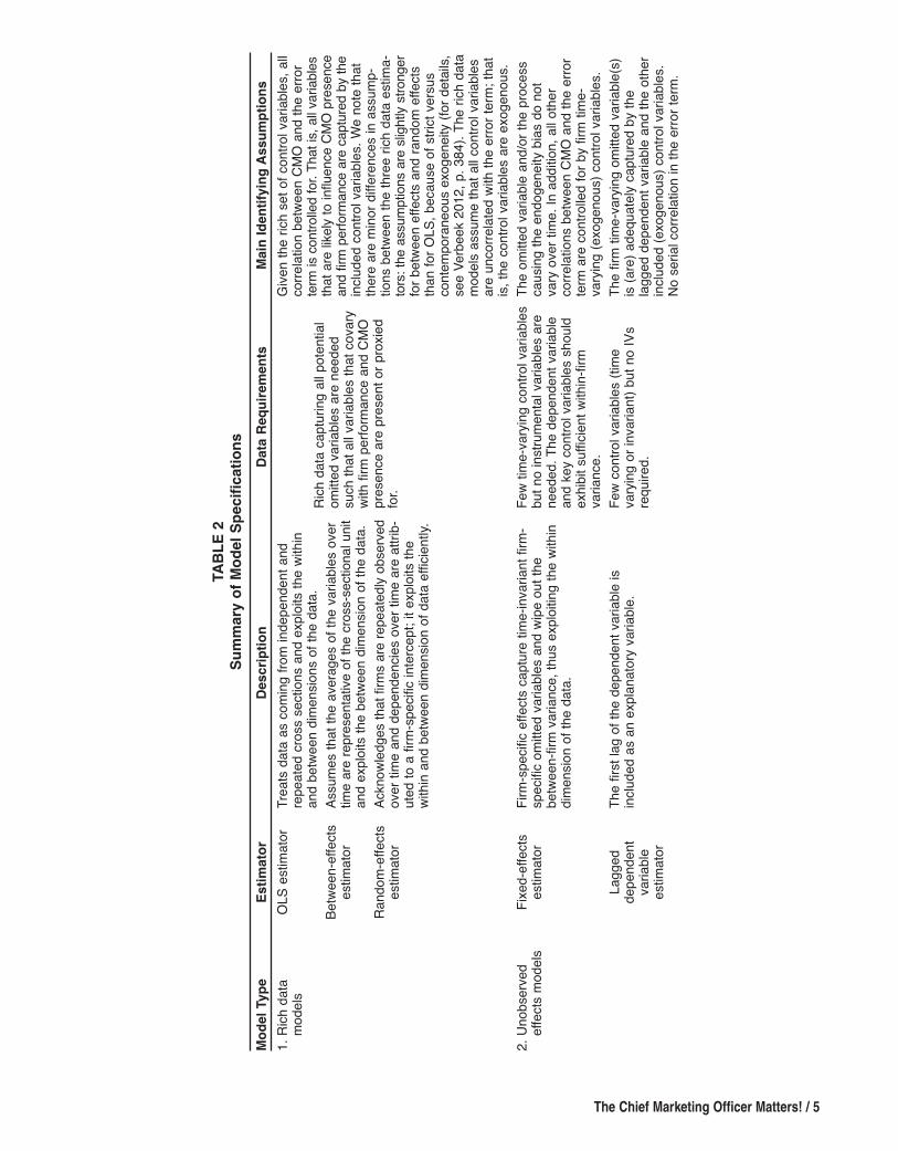
We discuss these models next, and we provide a summaryof the models, including their identification assumptions, inTable 2.Rich Data ModelsThe first approach is to collect an extensive data set suchthat no conceivable control variable (or proxies of such avariable) that correlates with both CMO presence and firmperformance is omitted; we refer to these models as richdata models. Such a data set would result in the modelshown in the following equation:(2) FPit = b0 + b1CMOit + b2Xit + �it,where the matrix Xit captures the time-invariant and time-variant control variables.3

If such an extensive set of control variables were avail-able, ordinary least squares (OLS), which exploits bothwithin and between dimensions of the data, could be usedto estimate the model (Section 7.8; Wooldridge 2002).Although we cannot claim with high confidence that noimportant variable is missing in our data, we report OLSresults (i.e., using Equation 2).

Moreover, if one repeatedly observes the same firmsover time, as we do in our panel data set, it is unrealistic toassume that the error terms for the same firm from differenttime periods are uncorrelated. Therefore, a popular alterna-tive to the model shown in Equation 2 is the random-effectspanel data model that assumes a composite error: �it = ai +uit, where ai is a firm-specific random error term that cap-tures unobserved firm-level effects and uit is the randomcomponent that varies across firms and over time. Randomeffects ai are assumed to be i.i.d. (usually a normal distribu-tion) and capture all correlation of the error terms overtime. Due to the random nature of firm-specific intercepts,the random-effects model exploits within and between vari-ance more efficiently than OLS.4

An alternative to the random-effects model is to onlyexploit differences between firms, thereby ignoring the time-series information. Such a model, referred to as the between-estimator model (e.g., Verbeek 2012, p. 382), requiresobtaining OLS estimates with firm-level means; that is,(3) FPi = b0 + b1CMOi + b2Xi + �i,where FPi denotes the average financial performance forfirm i across the years of observation (and similarly for the


other variables), and �i = ai + ui is the firm-level averagederror term.

The identifying assumptions of the between-estimatorare similar to those of the OLS and random-effects model:data are available on all important variables, and explana-tory variables are uncorrelated with the composite errorterm (that contains the missing variables). Although thismodel can be used to estimate the CMO effect (i.e., b1), it isgenerally preferable to use the random-effects estimator—particularly when the panel time-series dimension becomeslonger—because it exploits between and within dimensionsof the data. To be consistent with N&M (see their Table 3),we estimate the between-effects model as well.Unobserved Effects ModelsUnobserved effects models control for omitted variables byeither using firm-specific fixed effects or a lagged depen-dent variable as a control variable. These models exploit thefact that panel data have multiple observations for everyfirm, which enables modeling firm-specific intercepts orstate dependence through a lagged dependent variable.5Building on the model shown in Equation 2, the fixed-effects model includes the firm-specific intercept ai; that is,(4) FPit = ai + b1CMOit + b2Xit + uit,where ai are now fixed unknown constants and uit is i.i.d.over firms and time.

Typically, the firm-specific intercepts are not estimated;instead, the fixed-effects approach usually estimates themodel in deviations from firm-level means. Thus, the fixed-effects model does not require the assumption that CMOit isuncorrelated with ai. However, it does require the assumptionthat E(CMOit ¥ uis) = 0 for all s, t (and similarly for Xit) sothat the regressors are strictly exogenous. Thus, the identi-fying assumptions underlying the fixed-effects model arethat (1) the omitted variable(s) is (are) time invariant (i.e.,the firm-specific intercept captures the omitted variable[s])and (2) there is enough variance in the dependent variableas well as the focal endogenous variable within firms toallow estimation of its effect (i.e., the focal endogenousvariable— in our case, CMO presence—is identified onlythrough within-firm variation). We note that after includingfirm fixed effects, all time-invariant between-firm variationis removed. Typically, when the time dimension is short(e.g., as in Zhang and Liu 2012, in which they have sevendaily observations for all units of analysis), the identifyingassumptions of a fixed-effects model are easy to justify.However, in our case, the sample period ranges from 5 to12 years; thus, the identifying assumptions for the fixed-effects model might not be easily defensible. Yet we believeit is worth exploring this model’s results as one set ofresults among others. We note that we also include timefixed effects in the model to tease out any unique year-to-

3Here, it is necessary to assume that E(CMOit ¥ �it) = 0 andE(Xit ¥ �it) = 0; (i.e., CMOit and Xit are exogenous) and some othermild regularity conditions (e.g., Verbeek 2012, p. 373). In otherwords, we would need to assume that the set of control variablescaptures all unobserved variation that would otherwise be part ofthe error term correlating with CMO. All remaining unobservedvariation in the error term �it only correlates with the DV (i.e.,firm performance FPit) but not systematically with CMOit or Xit.

4As is common, we use feasible generalized least squares toestimate the random-effects model, where it is typically requiredthat E(CMOit ¥ uis) = 0 and E(Xit ¥ uis) = 0 for all s, t (i.e., strictexogeneity), and E(CMOi ¥ ai) = 0 and E(Xi ¥ ai) = 0 (e.g., Ver-beek 2012, p. 384).

5In theory, one can specify a model with both firm-specifictime-invariant effects and a lagged DV, as we do subsequently inEquation 7. However, estimating such a model requires strongassumptions (e.g., Nickell 1981), as we discuss in the “Panel Inter-nal Instruments Models” section.


Model Type

Estimator

Description

Data Requirements

Main Identifying Assumptions

1. Rich

data

models

OLS estim

ator

Treats data as coming

from

independent and

repeated cross sections and exploits the within

and between dim

ensio

ns of the data.

Rich data capturing

all p

otential

omitte

d variable

s are needed

such that all v

ariab

les that covary

with firm performance and CMO

presence are present or proxie

dfor.

Given the rich set of control variab

les, all

corre

lation

betwe

en CMO and the error

term is co

ntrolled for. That is, all variab

lesthat are lik

ely to influence CMO presence

and firm performance are ca

ptured by the

includ

ed control variab

les. W

e note that

there are mino

r diffe

rences in assum

p-tions betwe

en the three rich data estima-

tors: the assum

ption

s are sligh

tly stronger

for betwe

en effects

and random

effects

than for O

LS, because of strict versus

contem

poraneous e

xogeneity (for details,

see Verbeek 2012, p. 384). The rich data

models

assum

e that all c

ontrol variab

lesare uncorre

lated with the error term; that

is, the control variab

les are exogenous.

Between-effects

estim

ator

Assumes that the averages of the variab

les over

time are representative of the cross-sectional unit

and explo

its the between dim

ensio

n of the data.

Random

-effects

estim

ator

Acknow

ledges that firm

s are repeatedly observed

over time and dependencie

s over time are attrib-

uted to a firm-specific intercept; it exploits the

within and between dim

ensio

n of data efficien

tly.

2. Unobserved

effects

models

Fixed-effects

estim

ator

Firm-specific effects

capture time-inv

arian

t firm

-specific

omitte

d variable

s and wipe out the

between-firm varian

ce, thus explo

iting the within

dimensio

n of the data.

Few tim

e-varying

control variab

lesbut no ins

trumental variab

les are

needed. The dependent variab

leand key control variab

les should

exhib

it suffic

ient w

ithin-firm

variance.

The om

itted variable

and/or the process

causing

the endogeneity bias

do not

vary over time. In additio

n, all o

ther

corre

lation

s between CM

O and the error

term are controlled for by firm time-

varying

(exogenous) control variab

les.

Lagged

dependent

variable

estim

ator

The first lag

of the dependent variab

le is

includ

ed as an explan

atory variable

.Few control variab

les (time

varying

or invarian

t) but no IVs

required.

The firm time-varying

omitte

d variable

(s)

is (are) adequately

captured by the

lagged dependent variab

le and the other

includ

ed (exogenous) control variab

les.

No serial correlation

in the error term.

TABLE 2

Summary of Model Specifications


Model Type

Estimator

Description

Data Requirements

Main Identifying Assumptions

3. IV

models

IV estimator usin

gtwo-sta

ge least

squares (2SL

S)

Treats data as coming

from

a cross section,

corre

cts for an endogeneity bias

by using

ins

trumental variab

les that correlate with the

endogenous regressor but not with the error

term, and exploits within and between

dimensio

ns of data.a

Data on IV and som

e control

variable

s (e.g., advertisin

g spend-

ing in our case) so that the

reliance on IV

can be reduced to

the extent possib

le.

It is necessary to conceptually identify

avalid instrum

ent m

eeting the ins

trument

relev

ance and exclus

ion restriction

(and

provide

theoretical jus

tification for instru-

ment rele

vance and the exclu

sion

restriction

). Identification of the ins

trument

requires d

eep ins

titutional knowledge and

information

on processes that determine

the endogenous regressor. The strength

of the ins

trument also

needs to be

assessed empirica

lly and com

munica

ted.

Two-sta

ge least-

squares random

effects

(2SL

SRE)

The panel nature of the data is explicitly

recog-

nized in additio

n to the IV(s); that is, 2SL

SRE

explo

its within and between dim

ensio

ns of data

efficiently.

4. Panel internal

instrument

models

Hausman and

Taylo

r (1981)

estim

ator

Based on similar idea as fixed-effects

estimation

(i.e., deviation

s from firm means can be used

to control for time-inv

arian

t unobserved effects

),uses both within and between dim

ensio

ns of the

data, and is potentially more efficien

t than fixed-

effects

estimators.

Few control variab

les (time-varying

or invariant) but no IV(s) are

needed.

Same assumption

s as the fixed-effects

estim

ator.

Blundell a

nd Bond

(1998, 1999)

generalized

method of

mom

ents

estim

ator

Relies on past valu

es of the endogenous

variable

s to construct (internal) IVs and can be

used in the presence of persis

tence wh

en other

such estimators (e.g., Arellano and Bo

nd 1991)

are not useful.

Lagged measures of the endogenous

variable

s (note that in additio

n to the

[lagged] C

MO variable

, the lagged

dependent variab

le is als

o endogenous

here) are good predictors of the change

in the endogenous variab

les but do not

corre

late with the change in the firm-

specific

erro

r term; som

e assumption

son serial correlation

are required.b

TABLE 2

Continued

a Endogeneity can arise

due to omitte

d variable

(s), sim

ultaneity, and/or measurement erro

r (e.g., W

ooldridg

e 2002). In our case, the expla

natory variab

le is a strategic choic

e variable

. Unle

ssdata on all im

portant determina

nts o

f the explan

atory v

ariab

le that also

affect the dependent variab

le are available, there is a potential endogeneity b

ias due to omitte

d variable

s. We note that

standard 2SLS treats data as c

oming

from

a cross s

ection. Thus, in the case of panel data, 2SLSR

E is potentially more efficient. In additio

n, when the endogenous independent variab

le is dis

crete

(0/1), 2S

LSRE

may still be applied; how

ever, dependin

g on the em

pirica

l context, a potentially more efficien

t approach is obtaine

d by assum

ing a probit model for the first stage. In that case,

various IV

estimators can be applied (e.g., Wooldridg

e 2002, procedures 18.1 or 18.4). W

e adapt the control function approach outlin

ed in procedure 18.4 of W

ooldridg

e (2002) in Model 7.

b As s

hould

be evide

nt, the intuitio

n behin

d the IV that is param

ount in the IV models

is lost in panel in

ternal ins

truments models

; thus, from a co

nceptual sta

ndpoint, it is usually d

ifficult to jus

tifythe ins

trument derive

d from lagged measures or changes in lagged measures (also

see Roodm

an 2009).

Notes: The descriptions, identifying

assum

ption

s, and suggestions in this table

should

be vie

wed as ru

les of thumb and/or heuristics that we develop

ed from

our re

ading

of the literature and

experience with data.


TABLE 3

Correlations and Descriptive Statistics (Based on Sample 4)

Correlations

Variables 1 2 3 4 5 6 7 8 9 10 11 12 13 14 15 16

1. C

MO presence 1.00

2. Tobin’s q .14 1.00

3. Innovation

.16 .16 1.00

4. D

ifferentiation

–.02 .08 –.24 1.00

5. C

orporate branding

.06 .03 .09 –.16 1.00

6. Total div

ersifica

tion –.01 –.17 –.14 –.04 –.13 1.00

7. C

EO tenure .02 .12 .02 –.15 .18 –.04 1.00

8. O

utsid

er CEO

.03 –.05 .02 .16 –.03 .08 –.12

1.00

9. M

arket concentration .06 –.05 .17 –.02 –.16 .00 –.03

.01 1.00

10. Log(num

ber of emplo

yees) .04 –.02 –.20 .08 –.07 .25 –.11

–.08 .07 1.00

11. C

OO presence –.03 .04 –.06 .06 –.02 –.07 .10

.01 –.01 –.05 1.00

12. R

eturn on assets –.04 .25 –.45 .10 .00 –.03 .03

–.08 –.20 .14 –.02 1.00

13. S

ales grow

th .03 .34 .06 –.04 –.03 –.07 .06 .01 –.01 –.11

.07 .14 1.00

14. Tobin’s q (t – 1) .11 .50 .10 .05 .03 –.12 .03

–.01 –.05 –.07 .02 .13 .38 1.00

15. S

ystematic risk .03 .01 .14 –.10 .16 –.07 .00

.06 –.07 –.10 –.03 –.17 .05 .05 1.00

16. Idio

syncratic risk

.05 .06 .13 –.04 .07 –.12 –.04 .15 –.02 –.38 .03 –.25 .11 .16 .25 1.00

Summary Statistics

M .36 .50 –.03 .02 .43 .49 86.7 .29

508 2.16 .29 .07 .02 .76 1.04 .02

Mdn

.00 .11 –.01 .00 .00 .00 60.0 .00

381 1.91 .00 .06 –.01 .14 1.03 .02

SD .48 1.40 .10 .04 .50 .50 85.3 .45

453 1.53 .45 .16 .22 3.39 .39 .01

Max 1.00 12.9 .65 .26 1.00 1.00 492

1.00

4306 6.14 1.00 .77 2.42 78.5 2.73 .12

Min .00 –2.08 –.39 –.04 .00 .00 1.00

.00 .04 –1.68 .00 –2.14 –.86 –2.16 –1.17 .01

Notes: Following N&M

, Tobin’s q, innovation, diffe

rentiation

, return on assets, sales

growth, and Tobin’s q (t – 1) are the raw value

s les

s the median

valu

es at the tw

o-dig

it Standard Industrial

Classifica

tion (SIC) level.

year fluctuations (e.g., boom and bust cycles that uniformlyinfluence all firms in our sample).6

Moreover, if one believes that current firm performanceis influenced by the past (e.g., past firm decisions, carry-over effects), the introduction of a lagged dependentvariable might control for otherwise omitted variables andeffects. Specifically, time-varying unobserved effects (asopposed to time-invariant unobserved effects, as in thefixed-effects model) can be captured by including thelagged dependent variable (in our case, firm performance)as an additional control variable in the model. We can rep-resent such a model as follows:(5) FPit = b0 + b1CMOit + b2Xit + rFPit – 1 + �it,where FPit – 1 is the firm performance of the previous timeperiod and is included in the set of control variables.

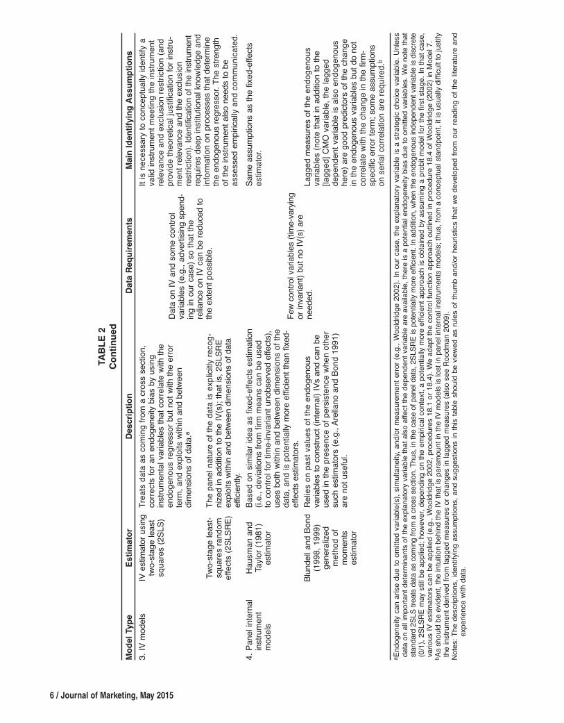
Including a lagged dependent variable as a controlvariable in the model typically reduces the autocorrelationin the model (but does not necessarily eliminate it). Consid-ering the model shown in Equation 5, the identifyingassumption for the CMO presence effect is that (1) theomitted variables are fully accounted for by the laggeddependent variable and (2) there is no serial correlation pre-sent in the error term �it. If these identifying assumptionsare met, the model would correct for firm-specific, time-varying omitted variables. Such a model exploits bothwithin- and between-firm variance and can be estimatedwith OLS, as we do subsequently.IV ModelsIf we cannot claim on theoretical grounds that the CMOeffect is uncorrelated with the error term �it in Equation 2(e.g., due to omitted variables), an alternate approach is tofind one or more IVs that correlate with the CMO variablebut not with the unobserved determinants of firm perfor-mance (that form part of the error term); that is, we mustfind IVs that meet the instrument relevance criterion andthe exclusion restriction (e.g., Angrist and Pischke 2009).The exclusion restriction can be thought of as introducingan additional equation to Equation 2 to explain/predictCMO presence:(6) CMOit = g0 + g1Zit + g2Xit + vit,where Zit is the IV that is excluded from Equation 2. Inaddition g1 must be ≠ 0 and, similar to Xit, Zit must beexogenous; that is, the IV must not be correlated with themodel error term in Equation 2 and E(Zit ¥ �it) = 0.

The use of a “good” IV enables one to “partition thevariation [in CMO presence] into that which can beregarded as clean or as though generated via experimentalmethods, and that which is contaminated and could result inan endogeneity bias” (Rossi 2014, p. 655). Unfortunately,good IVs can be difficult to find. Thus, Angrist and Pischke


(2009, p. 117) argue that finding IVs requires “a combina-tion of institutional knowledge and ideas about processesdetermining the variable of interest.” Likewise, Rossi(2014) notes that good IVs need to be justified using institu-tional knowledge because there is no true test for the qualityof IVs (for a discussion on statistical tests to examine thequality of instruments, see Rossi 2014).7

We use CMO prevalence among the sample firms’ peersas our primary IV. We define peer firms as those samplefirms that operate in the same primary two-digit StandardIndustrial Classification (SIC) code(s) as the focal firm andmeet other criteria (e.g., sales greater than $250 million in2002) for inclusion in our sample.8 Specifically, for each j =1, …, J SIC code (where J = 44 in our sample), if there arei = 1, 2, …, Nj firms in the code, the peer influence variablefor firm i (considering that the firm only belongs to one pri-mary SIC code j) would be the number of firms with aCMO in code j other than firm i divided by Nj – 1. More-over, if a firm belongs to multiple primary two-digit SICcodes, we calculate a weighted average of CMO prevalenceusing the number of sample firms in each primary SIC codeas the weight to calculate the IV. Most firms are listed inmultiple primary two-digit SIC codes, and these codes tendto change over time within a firm; therefore, the value ofthe peer CMO prevalence IV generally differs across firmsand over time.

To verify that CMO prevalence among peer firms is agood IV, we need to, on the one hand, demonstrate instru-ment relevance (i.e., that the IV predicts CMO presence)and, on the other hand, argue that the IV meets the exclu-sion restriction (i.e., establish that the IV does not correlatewith the error term that contains the omitted variables). Interms of instrument relevance, we need to conceptuallymake the case that CMO prevalence among peer firms cor-relates with CMO presence of the focal firm. Our argument

7Two other methods are also often used that parallel the use ofIV approaches: (1) control functions and (2) matching approaches.Similar to IV methods, the control function approach requires thatthe exclusion restriction is met and uses information from theexcluded variable to introduce a term for unobserved variables inthe regression specification; thus, a control variable is introducedfor the unobserved variables. Matching on the basis of the propen-sity score relies on creating an appropriate control group to com-pare with the treatment group and, thus, eliminates the need forinstrumental variable(s). If treatment and control groups can beobtained through matching, a difference-in-difference estimatorcan be used to obtain the causal effect of CMO presence. For acomparison of instrumental variables, control function, and match-ing procedures using propensity scores, see Heckman andNavarro-Lozano (2004).

8We used the Compustat Segments database to identify all pri-mary two-digit SIC codes to which our sample firms belonged ineach sample year. We note that while all firms have one primarytwo-digit SIC code assigned (referred to as principal two-digit SICcode hereinafter; see Tables WA1 and WA2 in the Web Appendix),many firms belong to more than just one primary SIC code, andwe use this information to calculate the IV. For example, in 2000,Procter & Gamble belonged to three primary two-digit SIC codes:20 (Food and Kindred Products), 26 (Paper and Allied Products),and 28 (Chemicals and Allied Products).

6Time-invariant variables in Xit are not allowed in the fixed-effects approach and are thus eliminated from the fixed-effectsmodel during estimation. If interest lies in such regressors, this is ahigh price to pay for choosing the fixed-effects model over, forexample, the random-effects model.

here rests on two primary premises. First, we argue that thefocal firms face similar market conditions as the peer firmsbecause the firms operate in the same industry(ies). Second,we assert that the expectations of the focal firm and the peerfirms are similar because we limit our sample to large firms(more than $250 million in sales in 2002) that invest in bothadvertising and R&D, functions often related to the market-ing department. Thus, similar market conditions and simi-larity of expectations should make the instrument relevant.

What remains to be argued is why our instrumentalvariable meets the exclusion restriction—that is, why it isuncorrelated with the omitted variables that affect the focalfirm’s financial performance. There are two types of omit-ted variables of concern. First, there are firm-level variablessuch as organizational culture (as discussed previously).Here, we argue that the peer firms collectively either cannotobserve or measure the focal firm’s omitted variable(s) orcannot act on those variable(s) strategically. For example,organizational processes and cultures that are difficult tomeasure and quantify are embedded in an organization’sfabric and thus become difficult to imitate (e.g., Granovet-ter 1985; Grewal and Slotegraaf 2007). Indeed, such pro-cesses are often difficult for the firms themselves to imitate(e.g., for the case of Saturn, see Kochan and Rubinstein2000). Consequently, many firms have open secrets that area source of competitive advantage (Barney 1991). In addi-tion, some sources of competitive advantage, such as patents,have legal protection and thus are difficult to imitate as well.Furthermore, because most of our sample firms belong toseveral primary two-digit SIC codes, a large number offirms is used to calculate a focal firm’s CMO prevalence-based instrument.9 Thus, it seems highly unlikely that peerfirms will take collective action against a single competitorand then also form other alliances similar in spirit to actagainst other competitors (which are also part of the otheralliances these firms form). We conclude that it is unlikelythat our instrument would relate to a focal firm’s omittedvariables (e.g., organizational culture) because (1) suchvariables may be difficult to assess and (2) collective actionis difficult to manage. Therefore, the instrument should beuncorrelated with the omitted variable and, thus, the errorterm that contains the omitted variable, thereby meeting theexclusion restriction.

The second type of omitted variables of concern areexogenous shocks that may systematically influence firmperformance and CMO prevalence over time, thereby creat-ing a correlation between CMO prevalence and the errorterm (which contains the exogenous shocks). Such shockscould include economy-wide boom and bust cycles, inwhich the health of the economy tends to dictate organiza-tional marketing emphases (e.g., Srinivasan, Lilien, andSridhar 2011). Time fixed effects should be able to proxy


shocks that are common across industries; thus, we includethese effects in our model specifications. However, suchexogenous shocks could also be specific to an industry in agiven time period; for example, as the price of crude oildrops, the profitability of allied industries is reduced. Con-sequently, allied industries might cut their marketing spend-ing, and perhaps also the CMO position, as their focusshifts from managing demand to cost cutting (e.g., Graham,Harvey, and Rajgopal 2005). Therefore, we also examine amodel specification in which we include time fixed effectsinteracted with industry-specific fixed effects as an additionalanalysis. In such a specification, the effect of CMO preva-lence on firm performance is identified by cross-sectionalvariation in CMO prevalence and firm performance withinindustries (SIC codes).

For our research, we use two IV approaches: First,given the panel structure of our data, we use the two-stageleast-squares random-effects estimator (2SLSRE). A poten-tially more efficient IV estimator may be obtained byappropriately accounting for the discreteness of the CMOvariable (e.g., Wooldridge 2002). Therefore, as a second IVmodel, we implement an estimation approach that accountsfor the discreteness of the CMO variable. That is, we use aprobit regression to estimate the first-stage regressionmodel in Equation 6 and then include the inverse Mills ratio(IMR) as a control function in a second-stage random-effects regression to estimate Equation 2 (see Wooldridge2002, procedure 18.4, p. 631).10, 11

Panel Internal Instruments ModelsOur fourth set of models relies on the panel nature of thedata to obtain IVs (we use the term “internal instruments”for instruments that arise from transformations of theincluded control variables in the main Equation 2 and“external instruments” for instruments excluded from themain Equation 2; see the “IV Models” section). Panel inter-nal instruments models typically use some transformationof the endogenous variable (in our case, CMO presence)and other included exogenous variables to obtain instru-ments. Thus, no external instruments are required to esti-mate these models. We discuss and use the Hausman andTaylor (1981) and the Blundell and Bond (1998, 1999)approaches here.

9In several instances, we only have a few sample firms forminga peer group (i.e., primary two-digit SIC code industry). As arobustness check, we dropped peer groups with fewer than sevenfirms from our sample and repeated the IV models; our main find-ing that the estimated CMO effect is positive and significant forTobin’s q remained unchanged.

10We include dummy variables for the primary two-digit SICcodes (most firms belong to multiple primary two-digit SIC codes)to which each focal firm belongs as control variables in the first-stage regression (i.e., Equation 6) to account for SIC-based vari-ance in CMO presence. These industry dummy variables areexogenous because CMO presence is not the primary variable thatdetermines the firms’ presence in an industry (two-digit SIC code).We note that the CMO effect remains positive and significantwhen excluding these additional SIC-based control variables fromEquation 6.

11Following Wooldridge (2002, procedure 18.4, p. 631), weinclude CMO ¥ (pdf/cdf), where pdf/cdf is the IMR and (1 –CMO) ¥ (pdf/(1 – cdf)) in the second-stage model, where CMO =1 if the firm has a CMO and CMO = 0 otherwise. We note that thisapproach requires normality assumptions for the model errorterms.

Hausman and Taylor (1981; hereinafter, HT) propose analternative to the (firm-specific) fixed-effects model in thepresence of endogenous variables. In particular, HT showthat the panel structure of the data can be used to obtain IVswithout requiring the traditional exclusion restrictions. TheHT approach is built on the same idea as the fixed-effectsmodel: it assumes that the omitted variable(s) is (are) timeinvariant. Moreover, HT show that the idea can be extendedto construct mean-centered IVs that are computed from theset of regressors. The HT approach exploits both the withinand between dimensions of the data and allows for theinclusion of firm-specific random effects (HT; Verbeek2012).

Building on the HT framework, Arellano and Bover(1995) and Blundell and Bond (1998, 1999; hereinafter,BB), among others, propose a more general IV frameworkfor panel data models based on generalized method ofmoments (GMM) estimation. These models are particularlyuseful when both firm-specific intercepts and lagged depen-dent variables are included as control variables. In the BBmodel, lagged measures and/or changes in lagged measuresare used as instruments for the lagged dependent variable(in our case, firm performance) and other potentiallyendogenous variables. Considering the two unobservedheterogeneity models discussed previously (i.e., fixed-effects and lagged dependent variable models), an alternatespecification to Equations 4 and 5 would be a model thatincludes both a firm-specific error term and a lagged depen-dent variable; that is,(7) FPit = b0 + b1CMOit + b2Xit + rFPit – 1 + ai + uit,where ai and uit are both random terms defined as previ-ously.

The estimation challenge of this model is that FPit – 1depends on ai (i.e., the two are positively correlated) andFPit – 1 is “endogenous” (in addition to CMOit). Moreover,the endogeneity of FPit – 1 could bias the effect of the CMOvariable,12 and even a fixed-effects estimation, whichwould remove ai, would not solve the problem because thewithin-transformed lagged dependent variable is correlatedwith the within-transformed error (Nickell 1981; Verbeek2012, p. 397). Thus, an alternative estimation approach is totake the first difference (which also removes the firm-spe-cific error term ai), as shown in Equation 8:(8) FPit – FPit – 1 = b1(CMOit – CMOit – 1) + b2(Xit – Xit – 1)

+ b3(FPit – 1 – FPit – 2) + (uit – uit – 1).This model cannot be estimated using OLS because

FPit – 1 is correlated with uit – 1. Instead, the endogeneity ofthe differenced lagged dependent variable can be addressedby using lagged values of the dependent variable as IVsresulting in a GMM estimator (e.g., Arellano and Bond


1991). However, the resulting GMM estimator has oftenbeen found to be unreliable in empirical applicationsbecause the lagged instruments tend to be weakly correlatedwith subsequent first differences, especially when theendogenous variables (in our case, lagged firm performanceand CMO presence) are highly persistent (i.e., when there isserial correlation in these variables; BB). Thus, we mustrely on GMM estimators that break the persistence in thedata. Considering the various existing GMM estimators,BB’s seems to be the most popular (for a critique, seeRoodman 2009). In brief, the BB estimator considers Equa-tions 7 and 8 as a system of equations. That is, it uses thelagged differences of the dependent variable as instrumentsfor the equation in levels (i.e., Equation 7) as well as laggedlevels of the dependent variable as instruments for the equa-tion in first differences (i.e., Equation 8; see also Arellanoand Bover 1995) to control for the potential endogeneity ofthe lagged dependent variable. The resulting system is usu-ally estimated with a GMM approach. The validity of the(lagged) difference instruments for the levels equationsdepends on the assumption that changes in the dependentvariable are uncorrelated with ai, which is the case whenthe series is in a more or less steady state (e.g., Blundell andBond 1999, pp. 7–8; Verbeek 2012, p. 403).Overall Proposed Modeling ApproachThe model specifications discussed previously rely on vary-ing identifying assumptions and data requirements, as sum-marized in Table 2. Recognizing that there are many poten-tial models available, we suggest that researchers explorethe meaning of the various models’ identifying assumptionsin light of their context and then determine the appropriatespecifications (as opposed to mechanically estimating manypotential models and then only reporting the model[s] thatprovide[s] the best results, thus becoming, in the words ofAngrist and Pischke [2009, p. 28], “regression mechanics”).For example, if researchers believe that they have an endo-geneity problem of the first order and they can providestrong theoretical arguments for a good IV, the IV approachshould be preferred. Similarly, some assumptions may betoo strong for the specific situation a researcher faces (e.g.,in our case, considering that we have a 12-year panel ofannual firm data, it might be difficult to defend the fixed-effects assumption—i.e., that the cause for endogeneity ofthe CMO effect is time invariant), and thus such modelsmay be ruled out from a conceptual standpoint.

We also want to recognize that it is important to assessand discuss the robustness of the results to various identify-ing assumptions (e.g., using both internal and externalinstruments) and investigate the same phenomenon fromdifferent vantage points. Indeed, it is conceivable that dif-ferent models do not produce the same results. If that is thecase, a careful conceptual justification is required for theidentifying assumptions of the effect based on institutionalknowledge. Thus, researchers should view themselves asregression engineers as opposed to “regression mechanics”(Angrist and Pischke 2009, p. 28) and understand the mean-ing of the model identifying assumptions for their context.Upon developing such an understanding, regression engi-

12While the direction and magnitude of the potential bias in theCMO effect are difficult to predict beforehand, some evidenceexists in the literature that suggests that the estimated CMO effectmay be biased downward (i.e., we would underestimate the CMOeffect; see Keele and Kelly 2006).

neers should estimate and discuss a subset of models whoseidentifying assumptions make the most sense given the dataand problem context (e.g., the models we summarize inTable 2). If the findings are convergent and show robust-ness, they would strengthen belief in the conclusionsdrawn. However, if the findings are not convergent, carefulanalysis of the identifying assumptions is needed to assesswhich results, if any, to believe or whether a differentapproach (e.g., a longer time series or additional controlvariables) is necessary.

Samples and MeasuresIn a first step, we aimed to replicate N&M’s sample asclosely as possible. Thus, using the Compustat database andconsidering the five-year period 2000–2004, we identifiedfirms with sales of at least $250 million in 2002. From thisset, and in line with N&M, we retained only firms withoutmissing data on the various factors (e.g., advertising,R&D). Moreover, in N&M’s footnote 7, they provide abreakdown of their sample by principal two-digit SIC code.We only retained firms with principal two-digit SIC codesrepresented in N&M’s sample. Using N&M’s (p. 70) filters,and after repeated efforts, our first sample (referred to asSample 1 subsequently) consisted of 123 firms for which wewere able to collect complete data across the five sampleyears. In comparison, N&M’s sample comprises 167 firms.

We note that N&M excluded several firms/SIC codesfor which complete data were available for 2000–2004. Forexample, N&M excluded firms from the Food and KindredProducts industry (e.g., General Mills Inc., Hershey Co., Kel-logg Co.), the Transportation Equipment industry (e.g., FordMotor Co., General Motors Co., Oshkosh Corp.), and Miscel-laneous Manufacturing Industries (e.g., Mattel Inc., HasbroInc., Callaway Golf Co.). Therefore, we created Sample 2,which included these additional firms and principal two-digitSIC codes. The total number of firms included in Sample 2 is155. Tables WA1 and WA2 in the Web Appendix compareour samples with N&M’s in terms of principal SIC codes.

Moreover, since N&M’s study was conducted, addi-tional firm years have become available beyond 2004. Atthe time our research was initiated, the most recent yearwith full secondary data available was 2011. We thus cre-ated Samples 3 and 4 by adding as many firm years as pos-sible to Samples 1 and 2. We note that the overall number offirms is the same in Samples 1 and 3 (i.e., 123 firms) aswell as Samples 2 and 4 (i.e., 155 firms).13

CMO PresenceConsidering Sample 4, our most complete sample, the per-centage of firms with a CMO did not change significantlybetween 2000 and 2011: specifically, 35% of the samplefirms had a CMO in 2000, whereas 37% had one in 2011(the percentage of firms with a CMO ranged from 32% to40% throughout our 12 sample years). These percentagesare comparable to those reported by N&M: their CMO per-


centages ranged between 39% and 44%. We note, however,that although overall CMO prevalence across all firmsremained fairly stable during the 12 sample years, it variedsignificantly within our respective sample firms. For exam-ple, in Sample 4, the largest sample, 30% of the firms hadno CMO during the entire 12 years, 7% of the firms had aCMO during the entire 12 years, and 63% of the firms hada CMO during some years but not during others. In addi-tion, considering Sample 1, our smallest and the sampleclosest to N&M’s sample, 41% of the firms had no CMOduring the entire five years, 16% of the firms had a CMOduring the entire five years, and 42% of the firms had aCMO during some years and not during others. These num-bers compare reasonably well with N&M’s, in whichapproximately 66% of the firms showed no variance inCMO presence. We also conducted a simulation study,described in detail in the Appendix, which suggests that ourdata exhibit sufficient within-firm CMO variation over timeto estimate our models.MeasuresWe closely followed N&M’s data collection procedures,collecting all variables, including the control variables. Todo so, we used various secondary data sources, includingCOMPUSTAT, company websites, firms’ 10-Ks, and proxystatements retrieved via EDGAR, Bloomberg, and CapitalIQ. We included the following control variables in all ourmodels: innovation, differentiation, corporate branding,total diversification, CEO tenure, outsider CEO, marketconcentration, number of employees (log), chief operatingofficer (COO) presence, and return on assets. We alsoincluded sales growth as an additional control variable in allmodels except those in which sales growth is the perfor-mance measure. For detailed information on the data collec-tion procedures and variables, see N&M (pp. 71–72).14

Performance MeasuresThe CMO is posited to have both short- and long-term perfor-mance implications (e.g., Boyd, Chandy, and Cunha 2010).Thus, to assess whether and how CMO presence affectsfirm performance, we require a performance measure that isforward looking and cumulative. Moreover, given the crosssection of firms (i.e., organizational heterogeneity) included inour sample, the measure also must be generalizable and com-parable across (1) firms in many different industries and (2)firms that pursue different performance outcome goals.

Historically, most of the academic (marketing) researchinvestigating firm performance has employed accounting-

13We list the names of the firms included in the four samples inTables WA3 and WA4 in the Web Appendix.

14We excluded the two variables TMT marketing experienceand TMT general management experience from our models fortwo reasons. First, as in N&M’s case, biographical data wereavailable for only approximately 75% of the executives of thesample firms. Second, virtually all TMT members had generalmanagement experience, so the variable showed no variation (i.e.,it was 1 for almost all firms). We note, however, that when weestimated our models including the TMT marketing experiencevariable (based on data for approximately 75% of the executives),the CMO effect remained positive and significant in all but thebetween-effects model (using Sample 4).

based measures such as sales growth or return on invest-ments (e.g., Buzzell and Gale 1987; Jacobson 1990). How-ever, in the words of Anderson, Fornell, and Mazvancheryl(2004, p. 174), “such measures … contain little or no infor-mation about the future value of a firm.” Indeed, accounting-based measures assume that previous investments affectonly current-period earnings. Yet, in reality, most types offirm investments (e.g., employing a CMO) affect futureearnings as well (e.g., Geyskens, Gielens, and Dekimpe2002). Similarly, firms in the same industry may differ intheir short-term objectives (e.g., one may emphasize prof-itability and the other may stress growth), and thus, thegoals of the CMOs should differ across firms. Moreover,because of industry and firm differences in accounting prac-tices, a comparison of accounting-based measures (e.g., salesgrowth, return on investment) across industries and firms isproblematic (Anderson, Fornell, and Mazvancheryl 2004).

Capital market–based measures overcome these chal-lenges in several ways: (1) they capture both immediate andfuture firm performance; (2) they are organizational goalagnostic, permitting performance comparison across firmsthat pursue different performance goals (e.g., growth vs.profits); and (3) they are less affected by accounting con-ventions because they include the potential effect ofaccounting practice inconsistencies across industries whenevaluating expected future revenue streams (e.g., Amit andWernerfelt 1990). Thus, capital market–based measures(rather than accounting-based measures) seem appropriatefor the purpose of the study.

Consistent with N&M, we employ Tobin’s q as ourfocal performance outcome measure. Tobin’s q, the ratio ofa firm’s market value to the current replacement cost of itsassets (Tobin 1969), is a forward-looking, capital market–based measure of the value of a firm. It provides a measureof the premium (or discount) that the market is willing topay above (below) the replacement costs of a firm’s assets,thus capturing any above-normal returns expected from afirm’s collection of assets (Amit and Wernerfelt 1990).Another appealing feature of Tobin’s q is that it adjusts forexpected market risk; in other words, because Tobin’s qcombines capital market data with accounting data, itimplicitly uses the correct risk-adjusted discount rate andthus minimizes distortion (e.g., Amit and Wernerfelt 1990;Montgomery and Wernerfelt 1988).

In addition to Tobin’s q, we also consider the CMO’simpact on three other capital market–based performancemeasures: Jensen’s a, systematic risk, and idiosyncraticrisk. Jensen’s a (e.g., Aksoy et al. 2008; Jensen 1968; Lyon,Barber, and Tsai 1999) is the intercept derived from a riskmodel, usually the Fama–French (1993) three-factor modelaugmented with the momentum factor (Carhart 1997).Jensen’s a should be zero unless the firm has a value drivernot captured by the independent variables of the risk model(e.g., Jacobson and Mizik 2009); in other words, it capturesrisk-adjusted returns in excess of or below those predictedby the risk model.

Conceptual and empirical evidence suggests that marketing-related investments serve to reduce firm risk(e.g., McAlister, Srinivasan, and Kim 2007; Srivastava,


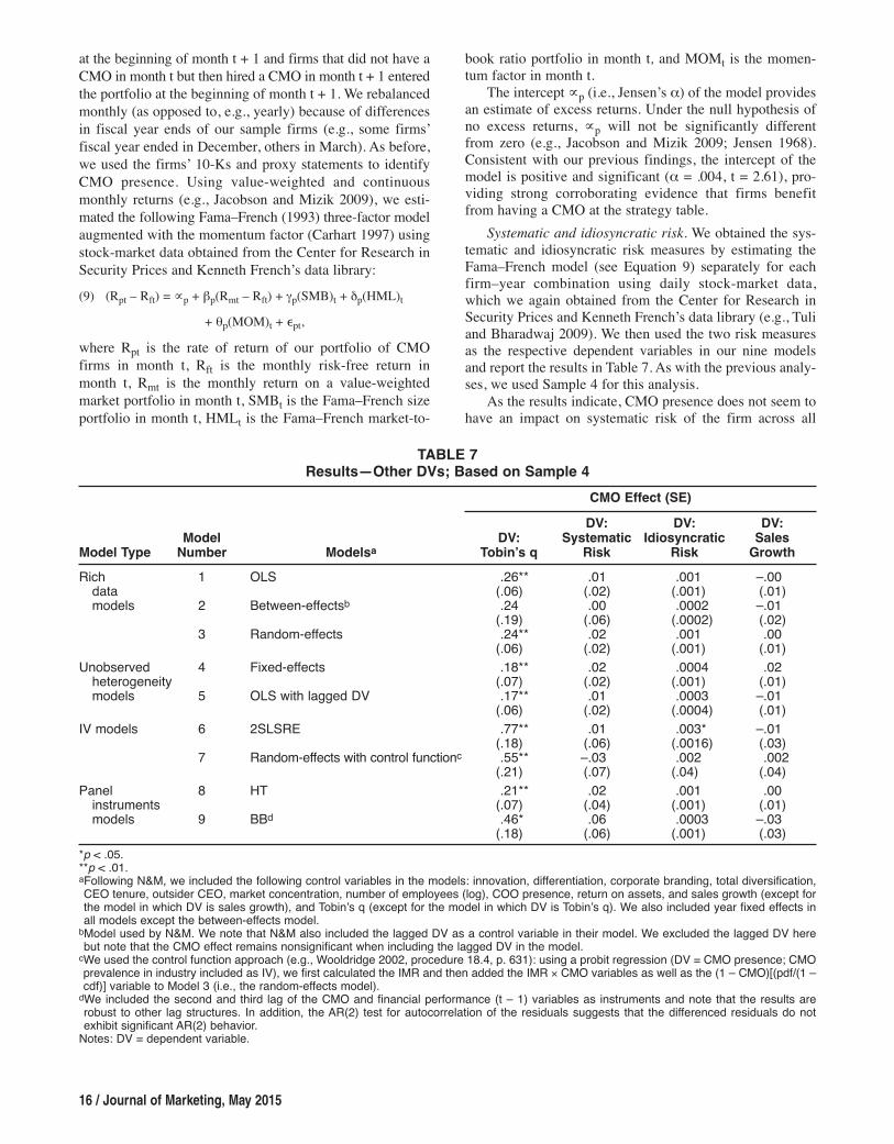
Shervani, and Fahey 1998; Tuli and Bharadwaj 2009).Therefore, it may be that CMO presence has risk-reducingproperties. Because both Tobin’s q and Jensen’s a are risk-adjusted measures (e.g., Aksoy et al. 2008; Madden, Fehle,and Fournier 2006; Montgomery and Wernerfelt 1988) and,in that sense, mask the effect of CMO presence on firm risk,we also investigate the CMO’s direct impact on a firm’ssystematic and idiosyncratic risk. Systematic risk representsthe degree to which a firm’s stock returns are a function ofmarket returns and thus are undiversifiable. In contrast,idiosyncratic risk represents risk specific to a firm that canbe eliminated from an investment portfolio (e.g., Lintner1965). Although there is an ongoing debate about the use-fulness of risk measures for predicting firm value (e.g.,Fama and French 1992; McAlister, Srinivasan, and Kim2007), both idiosyncratic and systematic risk are importantaspects of shareholder value (for a detailed discussion, seeTuli and Bharadwaj 2009), and we therefore include themas two additional performance measures.

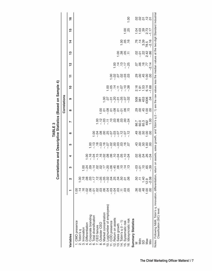
Finally, we report the impact of CMO presence on salesgrowth to be consistent with N&M, who used both Tobin’sq and sales growth as their performance measures. Follow-ing N&M, we calculate sales growth as the increase in salesas a proportion of the sales in the preceding year. However,because it is an accounting- and not a capital market–basedmeasure, we maintain that sales growth is not a suitablemeasure for the context of this study. Table 3 presents thedescriptive statistics.

ResultsThe CMO and Firm Tobin’s q

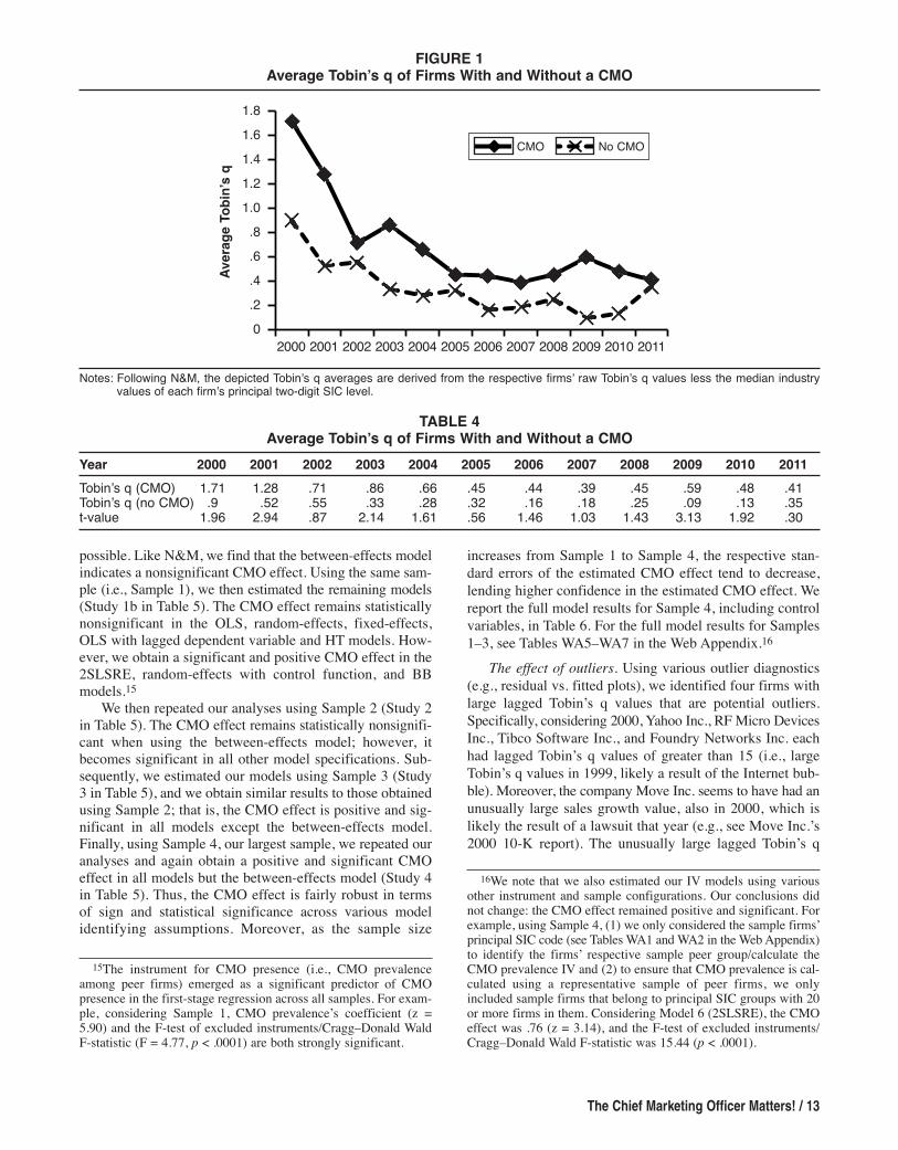
Model-free evidence. We first present model-free evi-dence regarding the relationship between CMO presenceand Tobin’s q. Considering Sample 4, our largest sample,and the average Tobin’s q across all time periods (i.e.,2000–2011), firms with a CMO in a given year, on average,displayed a Tobin’s q of .75, whereas firms without a CMOdisplayed a Tobin’s q of .36. This difference is statisticallysignificant (t = 5.37), suggesting that firms do benefit fromhaving a CMO among the TMT (we note that we couldhave also estimated this effect using the model shown inEquation 1). We also plotted the average Tobin’s q values byyear and CMO presence to capture the CMO effect in eachtime period. Figure 1 and Table 4 show the average Tobin’sq values of firms with and without a CMO across the 12years. Although the difference in Tobin’s q is not statisti-cally significant in each time period (except in 2000, 2001,2003, 2009, and 2010), Figure 1 again suggests that firmsindeed benefit from having a CMO at the strategy table: theline depicting Tobin’s q of CMO firms is always above theline depicting Tobin’s q of non-CMO firms. Notably, theaverage Tobin’s q of both types of firms (i.e., CMO andnon-CMO firms) was significantly greater in 2000 than insubsequent years, likely the result of the Internet bubble.

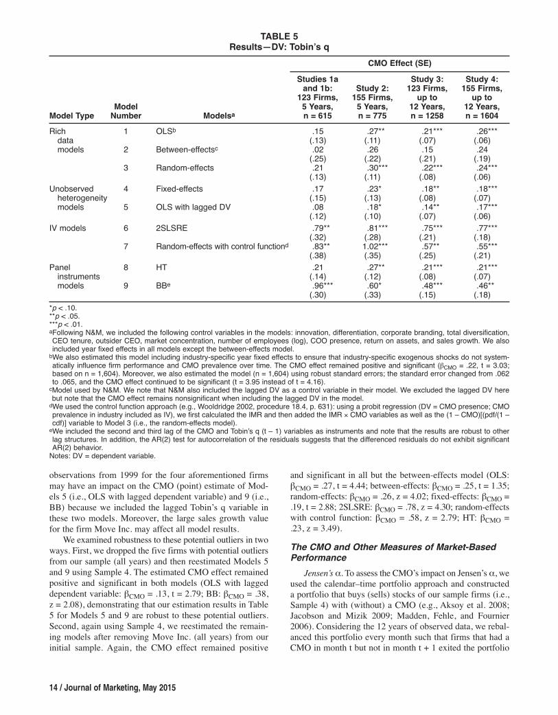
Model-based evidence. We begin our model-based analy-sis by estimating a between-effects model using Sample 1(Study 1a in Table 5) to replicate N&M’s work as closely as

possible. Like N&M, we find that the between-effects modelindicates a nonsignificant CMO effect. Using the same sam-ple (i.e., Sample 1), we then estimated the remaining models(Study 1b in Table 5). The CMO effect remains statisticallynonsignificant in the OLS, random-effects, fixed-effects,OLS with lagged dependent variable and HT models. How-ever, we obtain a significant and positive CMO effect in the2SLSRE, random-effects with control function, and BBmodels.15

We then repeated our analyses using Sample 2 (Study 2in Table 5). The CMO effect remains statistically nonsignifi-cant when using the between-effects model; however, itbecomes significant in all other model specifications. Sub-sequently, we estimated our models using Sample 3 (Study3 in Table 5), and we obtain similar results to those obtainedusing Sample 2; that is, the CMO effect is positive and sig-nificant in all models except the between-effects model.Finally, using Sample 4, our largest sample, we repeated ouranalyses and again obtain a positive and significant CMOeffect in all models but the between-effects model (Study 4in Table 5). Thus, the CMO effect is fairly robust in termsof sign and statistical significance across various modelidentifying assumptions. Moreover, as the sample size


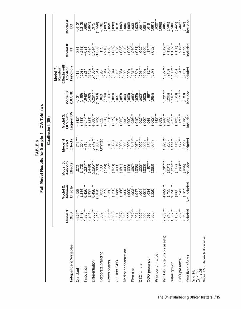
increases from Sample 1 to Sample 4, the respective stan-dard errors of the estimated CMO effect tend to decrease,lending higher confidence in the estimated CMO effect. Wereport the full model results for Sample 4, including controlvariables, in Table 6. For the full model results for Samples1–3, see Tables WA5–WA7 in the Web Appendix.16

The effect of outliers. Using various outlier diagnostics(e.g., residual vs. fitted plots), we identified four firms withlarge lagged Tobin’s q values that are potential outliers.Specifically, considering 2000, Yahoo Inc., RF Micro DevicesInc., Tibco Software Inc., and Foundry Networks Inc. eachhad lagged Tobin’s q values of greater than 15 (i.e., largeTobin’s q values in 1999, likely a result of the Internet bub-ble). Moreover, the company Move Inc. seems to have had anunusually large sales growth value, also in 2000, which islikely the result of a lawsuit that year (e.g., see Move Inc.’s2000 10-K report). The unusually large lagged Tobin’s q

15The instrument for CMO presence (i.e., CMO prevalenceamong peer firms) emerged as a significant predictor of CMOpresence in the first-stage regression across all samples. For exam-ple, considering Sample 1, CMO prevalence’s coefficient (z =5.90) and the F-test of excluded instruments/Cragg–Donald WaldF-statistic (F = 4.77, p < .0001) are both strongly significant.

16We note that we also estimated our IV models using variousother instrument and sample configurations. Our conclusions didnot change: the CMO effect remained positive and significant. Forexample, using Sample 4, (1) we only considered the sample firms’principal SIC code (see Tables WA1 and WA2 in the Web Appendix)to identify the firms’ respective sample peer group/calculate theCMO prevalence IV and (2) to ensure that CMO prevalence is cal-culated using a representative sample of peer firms, we onlyincluded sample firms that belong to principal SIC groups with 20or more firms in them. Considering Model 6 (2SLSRE), the CMOeffect was .76 (z = 3.14), and the F-test of excluded instruments/Cragg–Donald Wald F-statistic was 15.44 (p < .0001).

FIGURE 1Average Tobin’s q of Firms With and Without a CMO

2000 2001 2002 2003 2004 2005 2006 2007 2008 2009 2010 2011

1.81.61.41.21.0.8.6.4.20

Average Tobin’s q

CMO No CMO

Notes: Following N&M, the depicted Tobin’s q averages are derived from the respective firms’ raw Tobin’s q values less the median industryvalues of each firm’s principal two-digit SIC level.

TABLE 4Average Tobin’s q of Firms With and Without a CMO

Year 2000 2001 2002 2003 2004 2005 2006 2007 2008 2009 2010 2011Tobin’s q (CMO) 1.71 1.28 .71 .86 .66 .45 .44 .39 .45 .59 .48 .41Tobin’s q (no CMO) .9 .52 .55 .33 .28 .32 .16 .18 .25 .09 .13 .35t-value 1.96 2.94 .87 2.14 1.61 .56 1.46 1.03 1.43 3.13 1.92 .30

observations from 1999 for the four aforementioned firmsmay have an impact on the CMO (point) estimate of Mod-els 5 (i.e., OLS with lagged dependent variable) and 9 (i.e.,BB) because we included the lagged Tobin’s q variable inthese two models. Moreover, the large sales growth valuefor the firm Move Inc. may affect all model results.

We examined robustness to these potential outliers in twoways. First, we dropped the five firms with potential outliersfrom our sample (all years) and then reestimated Models 5and 9 using Sample 4. The estimated CMO effect remainedpositive and significant in both models (OLS with laggeddependent variable: bCMO = .13, t = 2.79; BB: bCMO = .38,z = 2.08), demonstrating that our estimation results in Table5 for Models 5 and 9 are robust to these potential outliers.Second, again using Sample 4, we reestimated the remain-ing models after removing Move Inc. (all years) from ourinitial sample. Again, the CMO effect remained positive


and significant in all but the between-effects model (OLS:bCMO = .27, t = 4.44; between-effects: bCMO = .25, t = 1.35;random-effects: bCMO = .26, z = 4.02; fixed-effects: bCMO =.19, t = 2.88; 2SLSRE: bCMO = .78, z = 4.30; random-effectswith control function: bCMO = .58, z = 2.79; HT: bCMO =.23, z = 3.49).The CMO and Other Measures of Market-BasedPerformance

Jensen’s a. To assess the CMO’s impact on Jensen’s a, weused the calendar–time portfolio approach and constructeda portfolio that buys (sells) stocks of our sample firms (i.e.,Sample 4) with (without) a CMO (e.g., Aksoy et al. 2008;Jacobson and Mizik 2009; Madden, Fehle, and Fournier2006). Considering the 12 years of observed data, we rebal-anced this portfolio every month such that firms that had aCMO in month t but not in month t + 1 exited the portfolio

TABLE 5Results—DV: Tobin’s q

CMO Effect (SE) Studies 1a Study 3: Study 4: and 1b: Study 2: 123 Firms, 155 Firms, 123 Firms, 155 Firms, up to up to Model 5 Years, 5 Years, 12 Years, 12 Years,Model Type Number Modelsa n = 615 n = 775 n = 1258 n = 1604Rich 1 OLSb .15 .27** .21*** .26***data (.13) (.11) (.07) (.06)models 2 Between-effectsc .02 .26 .15 .24 (.25) (.22) (.21) (.19) 3 Random-effects .21 .30*** .22*** .24*** (.13) (.11) (.08) (.06)

Unobserved 4 Fixed-effects .17 .23* .18** .18***heterogeneity (.15) (.13) (.08) (.07)models 5 OLS with lagged DV .08 .18* .14** .17*** (.12) (.10) (.07) (.06)

IV models 6 2SLSRE .79** .81*** .75*** .77*** (.32) (.28) (.21) (.18) 7 Random-effects with control functiond .83** 1.02*** .57** .55*** (.38) (.35) (.25) (.21)

Panel 8 HT .21 .27** .21*** .21***instruments (.14) (.12) (.08) (.07)models 9 BBe .96*** .60* .48*** .46** (.30) (.33) (.15) (.18)

*p < .10.**p < .05.***p < .01.aFollowing N&M, we included the following control variables in the models: innovation, differentiation, corporate branding, total diversification,CEO tenure, outsider CEO, market concentration, number of employees (log), COO presence, return on assets, and sales growth. We alsoincluded year fixed effects in all models except the between-effects model.bWe also estimated this model including industry-specific year fixed effects to ensure that industry-specific exogenous shocks do not system-atically influence firm performance and CMO prevalence over time. The CMO effect remained positive and significant (bCMO = .22, t = 3.03;based on n = 1,604). Moreover, we also estimated the model (n = 1,604) using robust standard errors; the standard error changed from .062to .065, and the CMO effect continued to be significant (t = 3.95 instead of t = 4.16).cModel used by N&M. We note that N&M also included the lagged DV as a control variable in their model. We excluded the lagged DV herebut note that the CMO effect remains nonsignificant when including the lagged DV in the model.dWe used the control function approach (e.g., Wooldridge 2002, procedure 18.4, p. 631): using a probit regression (DV = CMO presence; CMOprevalence in industry included as IV), we first calculated the IMR and then added the IMR ¥ CMO variables as well as the (1 – CMO)[(pdf/(1 –cdf)] variable to Model 3 (i.e., the random-effects model).eWe included the second and third lag of the CMO and Tobin’s q (t – 1) variables as instruments and note that the results are robust to otherlag structures. In addition, the AR(2) test for autocorrelation of the residuals suggests that the differenced residuals do not exhibit significantAR(2) behavior.Notes: DV = dependent variable.


TABLE 6

Full Model Results for Sample 4—

DV: Tobin’s q

Coeffiecient (SE)

Model 7:

Random

Model 2: Model 3: Model 4: Model 5: Effects with

Model 1:

Between Random Fixed OLS with Model 6: Control Model 8: Model 9:

Independent Variables OLS Effects Effects Effects Lagged DV 2SLSRE Function HT BB

Constant –.275** –.128 .072

.745***

–.242* –.121 –.11

9 .331

–.412*

(.148) (.214) (.172) (.201) (.138) (.189) (.203) (.218) (.213)

Innovation 4.376***

6.426***

1.234***

–.710

3.677***

1.046** .921* –.021

.660

(.341) (.937) (.446) (.534) (.321) (.460) (.515) (.484) (.651)

Differentiation

5.888*** 6.498***

5.295***

5.742***

4.608***

5.291***

5.133***

5.344***

.975

(.814) (1.870) (1.306) (1.866) (.762) (1.343) (1.351) (1.568) (1.558)

Corporate brandin

g .002

.053

.103 O

mitte

d –.022

.068

.093

.115 –.132

(.063) (.132) (.129) (.058) (.134) (.134) (.218) (.097)

Diversific

ation

–.285*** –.150

–.172** .010 –.221***

–.169** –.228*** –.083

–.058

(.063) (.156) (.078) (.088) (.059) (.080) (.084) (.082) (.098)

Outsider C

EO –.091 –.088

–.039

–.031

–.076

–.031

–.012

–.023

–.078

(.067) (.166) (.081) (.090) (.062) (.083) (.086) (.085) (.082)

Market concentration –.000

–.000

–.000

.000

–.000

–.000

–.000

.000

.000

(.000) (.000) (.000) (.000) (.000) (.000) (.000) (.000) (.000)

Firm size

.057***

.093** –.087** –.546***

.056***

–.089** –.081** –.260***

.033

(.021) (.047) (.038) (.072) (.019) (.039) (.039) (.051) (.033)

CEO tenure .002*** .001

.002***

.002***

.002***

.002***

.001***

.002***

.001**

(.000) (.001) (.000) (.000) (.000) (.000) (.000) (.000) (.001)

COO presence .060

.034

.167***

.171***

.065

.166** .182*** .174***

–.019

(.066) (.220) (.063) (.064) (.062) (.064) (.067) (.062) (.061)

Prior performance

.142***

.520***

(.009) (.068)

Profitability (return on assets) 2.758***

4.692***

1.761***

1.320***

2.368***

1.721***

1.827***

1.512***

.665

(.216) (.795) (.201) (.203) (.203) (.206) (.210) (.196) (.506)

Sales

growth 1.569*** 3.120***

1.214***

1.144***

.875***

1.167***

1.188***

1.152***

–.589

(.137) (.682) (.117) (.115) (.135) (.120) (.123) (.112) (.445)

CMO presence .259***

.241

.243***

.177***

.173***

.771***

.551***

.212***

.462**

(.062) (.187) (.064) (.066) (.058) (.183) (.212) (.065) (.182)

Year fixed effects

Includ

ed Not Inclu

ded Inclu

ded Inclu

ded Inclu

ded Inclu

ded Inclu

ded Inclu

ded Inclu

ded

*p< .10.

**p< .05.

***p< .01.

Notes: DV

= dependent variab

le.

at the beginning of month t + 1 and firms that did not have aCMO in month t but then hired a CMO in month t + 1 enteredthe portfolio at the beginning of month t + 1. We rebalancedmonthly (as opposed to, e.g., yearly) because of differencesin fiscal year ends of our sample firms (e.g., some firms’fiscal year ended in December, others in March). As before,we used the firms’ 10-Ks and proxy statements to identifyCMO presence. Using value-weighted and continuousmonthly returns (e.g., Jacobson and Mizik 2009), we esti-mated the following Fama–French (1993) three-factor modelaugmented with the momentum factor (Carhart 1997) usingstock-market data obtained from the Center for Research inSecurity Prices and Kenneth French’s data library:(9) (Rpt – Rft) = µp + bp(Rmt – Rft) + gp(SMB)t + dp(HML)t

+ qp(MOM)t + �pt,where Rpt is the rate of return of our portfolio of CMOfirms in month t, Rft is the monthly risk-free return inmonth t, Rmt is the monthly return on a value-weightedmarket portfolio in month t, SMBt is the Fama–French sizeportfolio in month t, HMLt is the Fama–French market-to-


book ratio portfolio in month t, and MOMt is the momen-tum factor in month t.

The intercept µp (i.e., Jensen’s a) of the model providesan estimate of excess returns. Under the null hypothesis ofno excess returns, µp will not be significantly differentfrom zero (e.g., Jacobson and Mizik 2009; Jensen 1968).Consistent with our previous findings, the intercept of themodel is positive and significant (a = .004, t = 2.61), pro-viding strong corroborating evidence that firms benefitfrom having a CMO at the strategy table.

Systematic and idiosyncratic risk. We obtained the sys-tematic and idiosyncratic risk measures by estimating theFama–French model (see Equation 9) separately for eachfirm–year combination using daily stock-market data,which we again obtained from the Center for Research inSecurity Prices and Kenneth French’s data library (e.g., Tuliand Bharadwaj 2009). We then used the two risk measuresas the respective dependent variables in our nine modelsand report the results in Table 7. As with the previous analy-ses, we used Sample 4 for this analysis.

As the results indicate, CMO presence does not seem tohave an impact on systematic risk of the firm across all

TABLE 7Results—Other DVs; Based on Sample 4

CMO Effect (SE) DV: DV: DV: Model DV: Systematic Idiosyncratic SalesModel Type Number Modelsa Tobin’s q Risk Risk GrowthRich 1 OLS .26** .01 .001 –.00data (.06) (.02) (.001) (.01)models 2 Between-effectsb .24 .00 .0002 –.01 (.19) (.06) (.0002) (.02) 3 Random-effects .24** .02 .001 .00 (.06) (.02) (.001) (.01)

Unobserved 4 Fixed-effects .18** .02 .0004 .02heterogeneity (.07) (.02) (.001) (.01)models 5 OLS with lagged DV .17** .01 .0003 –.01 (.06) (.02) (.0004) (.01)

IV models 6 2SLSRE .77** .01 .003* –.01 (.18) (.06) (.0016) (.03) 7 Random-effects with control functionc .55** –.03 .002 .002 (.21) (.07) (.04) (.04)

Panel 8 HT .21** .02 .001 .00instruments (.07) (.04) (.001) (.01)models 9 BBd .46* .06 .0003 –.03 (.18) (.06) (.001) (.03)

*p < .05.**p < .01.aFollowing N&M, we included the following control variables in the models: innovation, differentiation, corporate branding, total diversification,CEO tenure, outsider CEO, market concentration, number of employees (log), COO presence, return on assets, and sales growth (except forthe model in which DV is sales growth), and Tobin’s q (except for the model in which DV is Tobin’s q). We also included year fixed effects inall models except the between-effects model.bModel used by N&M. We note that N&M also included the lagged DV as a control variable in their model. We excluded the lagged DV herebut note that the CMO effect remains nonsignificant when including the lagged DV in the model.cWe used the control function approach (e.g., Wooldridge 2002, procedure 18.4, p. 631): using a probit regression (DV = CMO presence; CMOprevalence in industry included as IV), we first calculated the IMR and then added the IMR ¥ CMO variables as well as the (1 – CMO)[(pdf/(1 –cdf)] variable to Model 3 (i.e., the random-effects model).dWe included the second and third lag of the CMO and financial performance (t – 1) variables as instruments and note that the results arerobust to other lag structures. In addition, the AR(2) test for autocorrelation of the residuals suggests that the differenced residuals do notexhibit significant AR(2) behavior.Notes: DV = dependent variable.

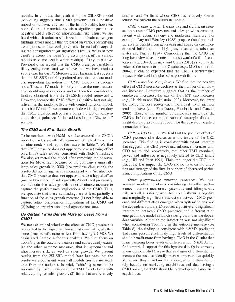
models. In contrast, the result from the 2SLSRE model(Model 6) suggests that CMO presence has a positiveimpact on idiosyncratic risk of the firm. Notably, however,none of the other models reveals a significant positive ornegative CMO effect on idiosyncratic risk. Thus, we arefaced with a situation in which we do not obtain convergentfindings across models that are based on various identifyingassumptions, as discussed previously. Instead of disregard-ing the nonsignificant (or significant) results, we must nowcarefully assess the identifying assumptions of the variousmodels used and decide which result(s), if any, to believe.Previously, we argued that the CMO presence variable islikely endogenous, and we believe that we have made astrong case for our IV. Moreover, the Hausman test suggeststhat the 2SLSRE model is preferred over the rich data mod-els, supporting the notion that CMO presence is endoge-nous. Thus, an IV model is likely to have the most reason-able identifying assumptions, and we therefore consider thefinding obtained from the 2SLSRE model noteworthy.However, because the CMO effect is (positive but) not sig-nificant in the random-effects with control function model,our other IV model, we cannot conclude with high certaintythat CMO presence indeed has a positive effect on idiosyn-cratic risk, a point we further address in the “Discussion”section.The CMO and Firm Sales GrowthTo be consistent with N&M, we also assessed the CMO’simpact on sales growth. We again use Sample 4 as well asall nine models and report the results in Table 7. We findthat CMO presence does not appear to have a (main) effecton a firm’s sales growth, consistent with N&M’s findings.We also estimated the model after removing the observa-tions for Move Inc., because of the company’s unusuallylarge sales growth in 2000 (see previous discussion); theresults did not change in any meaningful way. We also notethat CMO presence does not appear to have a lagged effect(one or two years) on sales growth. As outlined previously,we maintain that sales growth is not a suitable measure tocapture the performance implications of the CMO. Thus,we speculate that these nonfindings are at least partially afunction of the sales growth measure (1) not being able tocapture future performance implications of the CMO and(2) being an organizational goal agnostic measure.Do Certain Firms Benefit More (or Less) from aCMO?We next examined whether the effect of CMO presence ismoderated by firm-specific characteristics—that is, whethersome firms benefit more or less from having a CMO. Weagain used Sample 4 for this analysis. We first focus onTobin’s q as the outcome measure and subsequently exam-ine the other outcome measures, that is, systematic andidiosyncratic risk, as well as sales growth. We presentresults from the 2SLSRE model here but note that theresults were consistent across all models (results are avail-able from the authors). In brief, Tobin’s q seems to beimproved by CMO presence in the TMT for (1) firms withrelatively higher sales growth, (2) firms that are relatively


smaller, and (3) firms whose CEO has relatively shortertenure. We present the results in Table 8.

CMO ¥ sales growth. The positive and significant inter-action between CMO presence and sales growth seems con-sistent with extant strategy and marketing literature. Forexample, Day and Wensley (1988) propose that firms real-ize greater benefit from generating and acting on customer-oriented information in high-growth scenarios (also seeSlater and Narver 1994). Considering that the CMO haslong been viewed as the most direct steward of a firm’s cus-tomers (e.g., Boyd, Chandy, and Cunha 2010) as well as thevoice of the customer in the C-suite (e.g., McGovern et al.2004), it can be expected that the CMO’s performanceimpact is elevated in higher sales-growth firms.

CMO ¥ number of employees. We find that the positiveeffect of CMO presence declines as the number of employ-ees increases. Literature suggests that as the number ofemployees increases, the size of the TMT also increases(e.g., Haleblian and Finkelstein 1993). Moreover, the largerthe TMT, the less power each individual TMT membertends to have (e.g., Finkelstein, Hambrick, and Canella2009). Thus, as the number of employees increases, theCMO’s influence on organizational strategic directionmight decrease, providing support for the observed negativeinteraction effect.

CMO ¥ CEO tenure. We find that the positive effect ofCMO presence also decreases as the tenure of the CEOincreases. This finding is consistent with extant literaturethat suggests that CEO power and influence increases withCEO tenure and, conversely, that other TMT members’power and influence is negatively related to CEO tenure(e.g., Hill and Phan 1991). Thus, the longer the CEO is inplace, the less impact the CMO should have on the direc-tion and strategy of the firm, in support of decreased perfor-mance implications of the CMO.

Other performance outcome measures. We nextassessed moderating effects considering the other perfor-mance outcome measures, systematic and idiosyncraticrisk, as well as sales growth. As Table 8 shows, a negativeand marginally significant interaction between CMO pres-ence and differentiation emerged when systematic risk wasthe dependent variable. Moreover, a positive and significantinteraction between CMO presence and differentiationemerged in the model in which sales growth was the depen-dent variable. Although the interaction was not significantwhen considering Tobin’s q as the outcome measure (seeTable 8), the finding is consistent with N&M’s predictionthat firms pursuing relatively high levels of differentiationshould benefit more from having a CMO in the C-suite thanfirms pursuing lower levels of differentiation (N&M did notfind empirical support for this hypothesis). Quite correctlyin our opinion, N&M argue that strategies of differentiationincrease the need to identify market opportunities quickly.Moreover, they maintain that strategies of differentiationrely heavily on marketing capabilities and that having aCMO among the TMT should help develop and foster suchcapabilities.

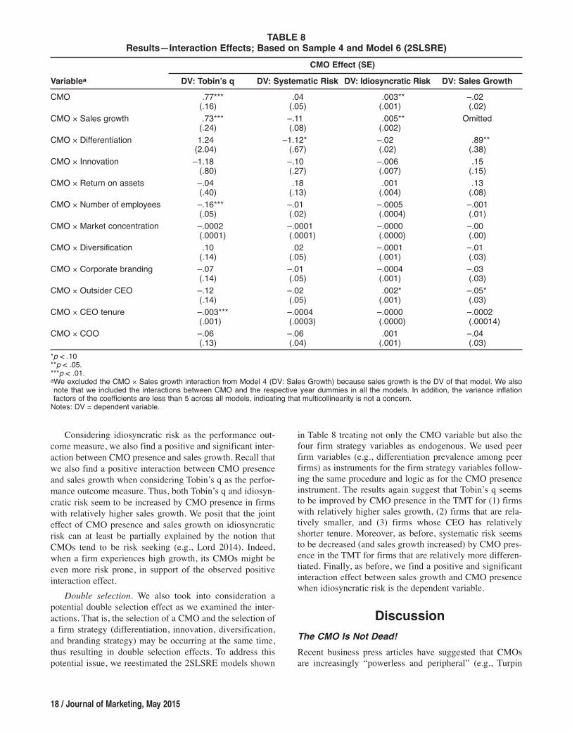
Considering idiosyncratic risk as the performance out-come measure, we also find a positive and significant inter-action between CMO presence and sales growth. Recall thatwe also find a positive interaction between CMO presenceand sales growth when considering Tobin’s q as the perfor-mance outcome measure. Thus, both Tobin’s q and idiosyn-cratic risk seem to be increased by CMO presence in firmswith relatively higher sales growth. We posit that the jointeffect of CMO presence and sales growth on idiosyncraticrisk can at least be partially explained by the notion thatCMOs tend to be risk seeking (e.g., Lord 2014). Indeed,when a firm experiences high growth, its CMOs might beeven more risk prone, in support of the observed positiveinteraction effect.

Double selection. We also took into consideration apotential double selection effect as we examined the inter-actions. That is, the selection of a CMO and the selection ofa firm strategy (differentiation, innovation, diversification,and branding strategy) may be occurring at the same time,thus resulting in double selection effects. To address thispotential issue, we reestimated the 2SLSRE models shown


in Table 8 treating not only the CMO variable but also thefour firm strategy variables as endogenous. We used peerfirm variables (e.g., differentiation prevalence among peerfirms) as instruments for the firm strategy variables follow-ing the same procedure and logic as for the CMO presenceinstrument. The results again suggest that Tobin’s q seemsto be improved by CMO presence in the TMT for (1) firmswith relatively higher sales growth, (2) firms that are rela-tively smaller, and (3) firms whose CEO has relativelyshorter tenure. Moreover, as before, systematic risk seemsto be decreased (and sales growth increased) by CMO pres-ence in the TMT for firms that are relatively more differen-tiated. Finally, as before, we find a positive and significantinteraction effect between sales growth and CMO presencewhen idiosyncratic risk is the dependent variable.

DiscussionThe CMO Is Not Dead!Recent business press articles have suggested that CMOsare increasingly “powerless and peripheral” (e.g., Turpin

TABLE 8Results—Interaction Effects; Based on Sample 4 and Model 6 (2SLSRE)

CMO Effect (SE)Variablea DV: Tobin’s q DV: Systematic Risk DV: Idiosyncratic Risk DV: Sales GrowthCMO .77*** .04 .003** –.02

(.16) (.05) (.001) (.02)CMO ¥ Sales growth .73*** –.11 .005** Omitted

(.24) (.08) (.002)CMO ¥ Differentiation 1.24 –1.12* –.02 .89**

(2.04) (.67) (.02) (.38)CMO ¥ Innovation –1.18 –.10 –.006 .15

(.80) (.27) (.007) (.15)CMO ¥ Return on assets –.04 .18 .001 .13

(.40) (.13) (.004) (.08)CMO ¥ Number of employees –.16*** –.01 –.0005 –.001

(.05) (.02) (.0004) (.01)CMO ¥ Market concentration –.0002 –.0001 –.0000 –.00

(.0001) (.0001) (.0000) (.00)CMO ¥ Diversification .10 .02 –.0001 –.01

(.14) (.05) (.001) (.03)CMO ¥ Corporate branding –.07 –.01 –.0004 –.03

(.14) (.05) (.001) (.03)CMO ¥ Outsider CEO –.12 –.02 .002* –.05*

(.14) (.05) (.001) (.03)CMO ¥ CEO tenure –.003*** –.0004 –.0000 –.0002

(.001) (.0003) (.0000) (.00014)CMO ¥ COO –.06 –.06 .001 –.04

(.13) (.04) (.001) (.03)*p < .10**p < .05.***p < .01. aWe excluded the CMO ¥ Sales growth interaction from Model 4 (DV: Sales Growth) because sales growth is the DV of that model. We alsonote that we included the interactions between CMO and the respective year dummies in all the models. In addition, the variance inflation factors of the coefficients are less than 5 across all models, indicating that multicollinearity is not a concern.Notes: DV = dependent variable.

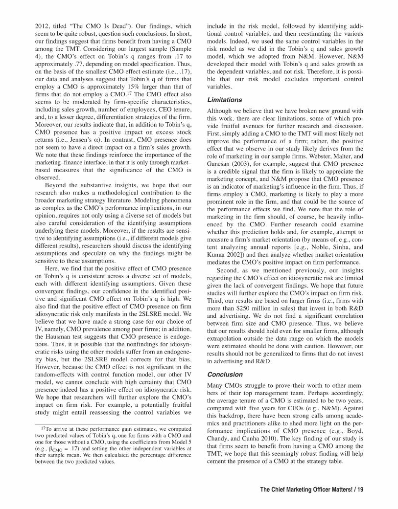
2012, titled “The CMO Is Dead”). Our findings, whichseem to be quite robust, question such conclusions. In short,our findings suggest that firms benefit from having a CMOamong the TMT. Considering our largest sample (Sample4), the CMO’s effect on Tobin’s q ranges from .17 toapproximately .77, depending on model specification. Thus,on the basis of the smallest CMO effect estimate (i.e., .17),our data and analyses suggest that Tobin’s q of firms thatemploy a CMO is approximately 15% larger than that offirms that do not employ a CMO.17 The CMO effect alsoseems to be moderated by firm-specific characteristics,including sales growth, number of employees, CEO tenure,and, to a lesser degree, differentiation strategies of the firm.Moreover, our results indicate that, in addition to Tobin’s q,CMO presence has a positive impact on excess stockreturns (i.e., Jensen’s a). In contrast, CMO presence doesnot seem to have a direct impact on a firm’s sales growth.We note that these findings reinforce the importance of themarketing–finance interface, in that it is only through market–based measures that the significance of the CMO isobserved.

Beyond the substantive insights, we hope that ourresearch also makes a methodological contribution to thebroader marketing strategy literature. Modeling phenomenaas complex as the CMO’s performance implications, in ouropinion, requires not only using a diverse set of models butalso careful consideration of the identifying assumptionsunderlying these models. Moreover, if the results are sensi-tive to identifying assumptions (i.e., if different models givedifferent results), researchers should discuss the identifyingassumptions and speculate on why the findings might besensitive to these assumptions.

Here, we find that the positive effect of CMO presenceon Tobin’s q is consistent across a diverse set of models,each with different identifying assumptions. Given theseconvergent findings, our confidence in the identified posi-tive and significant CMO effect on Tobin’s q is high. Wealso find that the positive effect of CMO presence on firmidiosyncratic risk only manifests in the 2SLSRE model. Webelieve that we have made a strong case for our choice ofIV, namely, CMO prevalence among peer firms; in addition,the Hausman test suggests that CMO presence is endoge-nous. Thus, it is possible that the nonfindings for idiosyn-cratic risks using the other models suffer from an endogene-ity bias, but the 2SLSRE model corrects for that bias.However, because the CMO effect is not significant in therandom-effects with control function model, our other IVmodel, we cannot conclude with high certainty that CMOpresence indeed has a positive effect on idiosyncratic risk.We hope that researchers will further explore the CMO’simpact on firm risk. For example, a potentially fruitfulstudy might entail reassessing the control variables we


include in the risk model, followed by identifying addi-tional control variables, and then reestimating the variousmodels. Indeed, we used the same control variables in therisk model as we did in the Tobin’s q and sales growthmodel, which we adopted from N&M. However, N&Mdeveloped their model with Tobin’s q and sales growth asthe dependent variables, and not risk. Therefore, it is possi-ble that our risk model excludes important controlvariables.LimitationsAlthough we believe that we have broken new ground withthis work, there are clear limitations, some of which pro-vide fruitful avenues for further research and discussion.First, simply adding a CMO to the TMT will most likely notimprove the performance of a firm; rather, the positiveeffect that we observe in our study likely derives from therole of marketing in our sample firms. Webster, Malter, andGanesan (2003), for example, suggest that CMO presenceis a credible signal that the firm is likely to appreciate themarketing concept, and N&M propose that CMO presenceis an indicator of marketing’s influence in the firm. Thus, iffirms employ a CMO, marketing is likely to play a moreprominent role in the firm, and that could be the source ofthe performance effects we find. We note that the role ofmarketing in the firm should, of course, be heavily influ-enced by the CMO. Further research could examinewhether this prediction holds and, for example, attempt tomeasure a firm’s market orientation (by means of, e.g., con-tent analyzing annual reports [e.g., Noble, Sinha, andKumar 2002]) and then analyze whether market orientationmediates the CMO’s positive impact on firm performance.

Second, as we mentioned previously, our insightsregarding the CMO’s effect on idiosyncratic risk are limitedgiven the lack of convergent findings. We hope that futurestudies will further explore the CMO’s impact on firm risk.Third, our results are based on larger firms (i.e., firms withmore than $250 million in sales) that invest in both R&Dand advertising. We do not find a significant correlationbetween firm size and CMO presence. Thus, we believethat our results should hold even for smaller firms, althoughextrapolation outside the data range on which the modelswere estimated should be done with caution. However, ourresults should not be generalized to firms that do not investin advertising and R&D.ConclusionMany CMOs struggle to prove their worth to other mem-bers of their top management team. Perhaps accordingly,the average tenure of a CMO is estimated to be two years,compared with five years for CEOs (e.g., N&M). Againstthis backdrop, there have been strong calls among acade-mics and practitioners alike to shed more light on the per-formance implications of CMO presence (e.g., Boyd,Chandy, and Cunha 2010). The key finding of our study isthat firms seem to benefit from having a CMO among theTMT; we hope that this seemingly robust finding will helpcement the presence of a CMO at the strategy table.

17To arrive at these performance gain estimates, we computedtwo predicted values of Tobin’s q, one for firms with a CMO andone for those without a CMO, using the coefficients from Model 5(e.g., bCMO = .17) and setting the other independent variables attheir sample mean. We then calculated the percentage differencebetween the two predicted values.

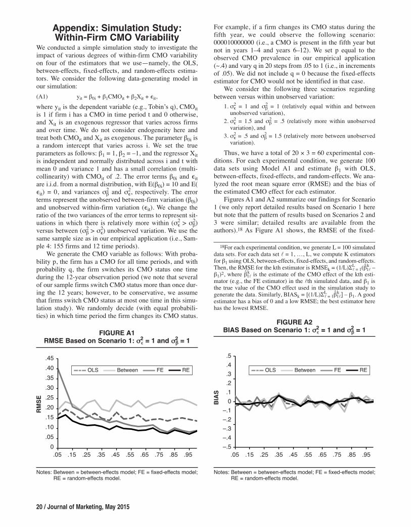
Appendix: Simulation Study:Within-Firm CMO Variability

We conducted a simple simulation study to investigate theimpact of various degrees of within-firm CMO variabilityon four of the estimators that we use—namely, the OLS,between-effects, fixed-effects, and random-effects estima-tors. We consider the following data-generating model inour simulation:(A1) yit = b0i + b1CMOit + b2Xit + �it,where yit is the dependent variable (e.g., Tobin’s q), CMOitis 1 if firm i has a CMO in time period t and 0 otherwise,and Xit is an exogenous regressor that varies across firmsand over time. We do not consider endogeneity here andtreat both CMOit and Xit as exogenous. The parameter b0i isa random intercept that varies across i. We set the trueparameters as follows: b1 = 1, b2 = –1, and the regressor Xitis independent and normally distributed across i and t withmean 0 and variance 1 and has a small correlation (multi-collinearity) with CMOit of .2. The error terms b0i and �itare i.i.d. from a normal distribution, with E(b0i) = 10 and E(�it) = 0, and variances s2

b and s2�, respectively. The errorterms represent the unobserved between-firm variation (b0i)and unobserved within-firm variation (�it). We change theratio of the two variances of the error terms to represent sit-uations in which there is relatively more within (s2� > s2

b)versus between (s2

b > s2�) unobserved variation. We use thesame sample size as in our empirical application (i.e., Sam-ple 4: 155 firms and 12 time periods).

We generate the CMO variable as follows: With proba-bility p, the firm has a CMO for all time periods, and withprobability q, the firm switches its CMO status one timeduring the 12-year observation period (we note that severalof our sample firms switch CMO status more than once dur-ing the 12 years; however, to be conservative, we assumethat firms switch CMO status at most one time in this simu-lation study). We randomly decide (with equal probabili-ties) in which time period the firm changes its CMO status.


For example, if a firm changes its CMO status during thefifth year, we could observe the following scenario:000010000000 (i.e., a CMO is present in the fifth year butnot in years 1–4 and years 6–12). We set p equal to theobserved CMO prevalence in our empirical application(~.4) and vary q in 20 steps from .05 to 1 (i.e., in incrementsof .05). We did not include q = 0 because the fixed-effectsestimator for CMO would not be identified in that case.

We consider the following three scenarios regardingbetween versus within unobserved variation:

1. s2� = 1 and s2b = 1 (relatively equal within and between

unobserved variation),2. s2� = 1.5 and s2

b = .5 (relatively more within unobservedvariation), and

3. s2� = .5 and s2b = 1.5 (relatively more between unobserved

variation).Thus, we have a total of 20 ¥ 3 = 60 experimental con-

ditions. For each experimental condition, we generate 100data sets using Model A1 and estimate b1 with OLS,between-effects, fixed-effects, and random-effects. We ana-lyzed the root mean square error (RMSE) and the bias ofthe estimated CMO effect for each estimator.

Figures A1 and A2 summarize our findings for Scenario1 (we only report detailed results based on Scenario 1 herebut note that the pattern of results based on Scenarios 2 and3 were similar; detailed results are available from theauthors).18 As Figure A1 shows, the RMSE of the fixed-

FIGURE A1RMSE Based on Scenario 1: s2� = 1 and s2b = 1

.05 .15 .25 .35 .45 .55 .65 .75 .85 .95

.45

.40

.35

.30

.25

.20

.15

.10

.050

RMSE

OLS Between FE RE

Notes: Between = between-effects model; FE = fixed-effects model;RE = random-effects model.

FIGURE A2BIAS Based on Scenario 1: s2� = 1 and s2b = 1

.05 .15 .25 .35 .45 .55 .65 .75 .85 .95

.5

.4

.3

.2

.10

–.1–.2–.3–.4–.5

BIAS

OLS Between FE RE

Notes: Between = between-effects model; FE = fixed-effects model;RE = random-effects model.

18For each experimental condition, we generate L = 100 simulateddata sets. For each data set = 1, …, L, we compute K estimatorsfor b1 using OLS, between-effects, fixed-effects, and random-effects.Then, the RMSE for the kth estimator is RMSEk = (1/L)SL

= 1(b̂k1 –

b1)2, where b̂k1 is the estimate of the CMO effect of the kth esti-

mator (e.g., the FE estimator) in the th simulated data, and b1 isthe true value of the CMO effect used in the simulation study togenerate the data. Similarly, BIASk = [(1/L)SL

= 1b̂k1] – b1. A good

estimator has a bias of 0 and a low RMSE; the best estimator herehas the lowest RMSE.

effects estimator is largest for small values of q; that is,when most firms (up to approximately q = 15%) do notchange CMO status across the 12 time periods. However,when approximately 20% of the firms change CMO statusonce during the 12 time periods, the between-effects esti-mator has the largest RMSE. For Scenarios 2 and 3 (resultsnot shown), we find similar patterns: the fixed-effects esti-mator has the largest RMSE for values of q up to 45% and10%, respectively. Notably, the random-effects estimatoralways has the lowest RMSE, and OLS always has a lowerRMSE than the between-effects estimator. Moreover, Fig-ure A2 shows that, across all values of q, the CMO effect isestimated in an approximately unbiased way by all fourestimators. That is, even when only 5% of the firms switchCMO status once, we still obtain an approximately unbi-


ased estimate of the CMO effect (Scenarios 2 and 3 yieldedalmost identical results).

In our empirical application (considering Sample 4), 37%of the firms do not switch CMO status and 63% of the firmsswitch CMO status once or more. In our simulation study,the fixed-effects, random-effects, and (to a lesser degree)OLS estimators always behave well for levels of q > 60%.The between-effects estimator, however, has a fairly highRMSE for all levels of q. Whether fixed-effects, random-effects, and OLS estimators are more or less efficient thanbetween-effects estimators in the end is an empirical ques-tion. However, our simulation results indicate that fixed-effects, random-effects, and OLS estimators indeed seem tobe more efficient than the between-effects estimator giventhe context of our CMO study.

Fama, Eugene F. and Kenneth R. French (1992), “The Cross Sectionof Expected Stock Returns,” Journal of Finance, 47 (2), 427–65.

——— and ——— (1993), “Common Risk Factors in the Returnson Stocks and Bonds,” Journal of Finance Economics, 33 (1),3–56.

Finkelstein, Sydney, Donald C. Hambrick, and Albert A. CannellaJr. (2009), Strategic Leadership: Theory and Research onExecutives, Top Management Teams, and Boards. New York:Oxford University Press.

Frazier, Mya (2007), “CMOs Rapped for Having Zero Impact onSales,” Advertising Age, 78 (July), 1.

Geyskens, Inge, Katrijn Gielens, and Marnik G. Dekimpe (2002),“The Market Valuation of Internet Channel Additions,” Jour-nal of Marketing, 66 (April), 102–119.

Graham, John R., Campbell R. Harvey, and Shiva Rajgopal(2005), “The Economic Implications of Corporate FinancialReporting,” Journal of Accounting and Economics, 40 (1–3),3–73.

Granovetter, Mark (1985), “Economic Action and Social Struc-ture: The Problem of Embeddedness,” American Journal ofSociology, 91 (3), 481–510.

Grewal, Rajdeep and Rebecca J. Slotegraaf (2007), “Embedded-ness of Organizational Capabilities,” Decision Sciences, 38 (3),451–88.

Haleblian, Jerayr and Sydney Finkelstein (1993), “Top Manage-ment Team Size, CEO Dominance, and Firm Performance: TheModerating Roles of Environmental Turbulence and Discre-tion,” Academy of Management Journal, 36 (4), 844–63.

Hambrick, Donald C. and Gregory D.S. Fukutomi (1991), “TheSeasons of a CEO’s Tenure,” Academy of Management Review,16 (4), 719–42.

Hausman, Jerry A. and William E. Taylor (1981), “Panel Data andUnobservable Individual Effects,” Econometrica, 43 (6),1377–98.

Heckman, James and Salvador Navarro-Lozano (2004), “UsingMatching, Instrumental Variables, and Control Functions toEstimate Economic Choice Models,” Review of Economics andStatistics, 36 (1), 30–57.

Hill, Charles W.L. and Phillip Phan (1991), “CEO Tenure as aDeterminant of CEO Pay,” Academy of Management Journal,34 (3), 707–717.

Jacobson, Robert (1990), “Unobservable Effects and BusinessPerformance,” Marketing Science, 9 (1), 74–85.

——— and Natalie Mizik (2009), “The Financial Markets and Cus-tomer Satisfaction: Reexamining Possible Financial MarketMispricing of Customer Satisfaction,” Marketing Science, 28(5), 810–19.

REFERENCESAksoy, Lerzan, Bruce Cooil, Christopher Groening, Timothy L.

Keiningham, and Atakan Yalçın (2008), “The Long-TermStock Market Valuation of Customer Satisfaction,” Journal ofMarketing, 72 (July), 105–122.

Amit, Raphael and Birger Wernerfelt (1990), “Why Do FirmsReduce Business Risk?” Academy of Management Journal, 33(3), 520–33.

Anderson, Eugene W., Claes Fornell, and Sanal K. Mazvancheryl(2004), “Customer Satisfaction and Shareholder Value,” Jour-nal of Marketing, 68 (October), 172–85.

Angrist, Joshua D. and Jӧrn-Steffen Pischke (2009), Mostly Harm-less Econometrics: An Empiricist’s Companion. Princeton, NJ:Princeton University Press.

——— and ——— (2010), “The Credibility Revolution in Empiri-cal Economics: How Better Research Design Is Taking the Conout of Econometrics,” Journal of Economic Literature, 24 (2),3–30.

Arellano, Manuel and Stephen R. Bond (1991), “Some Tests ofSpecification for Panel Data: Monte Carlo Evidence and anApplication to Employment Equations,” Review of EconomicStudies, 58 (2), 277–97.

——— and Olympia Bover (1995), “Another Look at the Instrumental-Variable Estimation of Error-Components Mod-els,” Journal of Econometrics, 68 (1), 29–51.

Barney, Jay (1991), “Firm Resources and Sustained CompetitiveAdvantage,” Journal of Management, 17 (1), 99–120.

Barta, Thomas (2011), “Do Firms Need CMOs?” (accessed March3, 2014), [available at http://www.thomasbarta.com/do-firms-need-cmos/].

Blundell, Richard and Stephen Bond (1998), “Initial Conditionsand Moment Restrictions in Dynamic Panel Data Models,”Journal of Econometrics, 87 (1), 115–43.

——— and ——— (1999), “GMM Estimation with Persistent PanelData: An Application to Production Function Estimation,”Working Paper Series No. W99/4, The Institute for Fiscal Stud-ies, London.

Boyd, D. Eric, Rajesh K. Chandy, and Marcus Cunha Jr. (2010),“When Do Chief Marketing Officers Affect Firm Value? ACustomer Power Explanation,” Journal of MarketingResearch, 47 (December), 1162–76.

Buzzell, Robert D. and Bradley T. Gale (1987), The PIMS Princi-ples. New York: The Free Press.

Carhart, Mark M. (1997), “On Persistence in Mutual Fund Perfor-mance,” Journal of Finance, 52 (1), 57–82.

Day, George S. and Robin Wensley (1988), “Assessing Advan-tage: A Framework for Diagnosing Competitive Superiority,”Journal of Marketing, 52 (April), 1–20.

Jensen, Michael C. (1968), “The Performance of Mutual Funds inthe Period 1945–1964,” Journal of Finance, 23 (2), 389–416.

Keele, Luke and Nathan J. Kelly (2006), “Dynamic Models forDynamic Theories: The Ins and Outs of Lagged DependentVariables,” International Journal of Public Opinion Research,14 (2), 186–205.

Kerin, Roger A. (2005), “Strategic Marketing and the CMO,” in“Marketing Renaissance: Opportunities and Imperatives forImproving Marketing Thought, Practice, and Infrastructure,”Journal of Marketing, 69 (October), 12–14.

Kochan, Thomas A. and Saul A. Rubinstein (2000), “Toward aStakeholder Theory of the Firm: The Saturn Partnership,”Organization Science, 11 (4), 367–86.

Leamer, Edward E. (1983), “Let’s Take the Con out of Economet-rics,” American Economic Review, 73 (1), 31–43.

Lintner, John (1965), “The Valuation of Risk Assets and the Selec-tion of Risky Investments in Stock Portfolios and Capital Bud-gets,” Review of Economics and Statistics, 47 (1), 13–37.

Lord, Joanna (2014), “20 Traits of Successful CMOs,” Marketing-Land, (February 11), (accessed October 25, 2014), [available athttp://marketingland.com/20-traits-successful-cmos-2-73629.

Lyon, John D., Brad M. Barber, and Chih-Ling Tsai (1999),“Improved Methods for Tests of Long-Run Abnormal StockReturns, Journal of Finance, 54 (1), 165–201.

Madden, Thomas J., Frank Fehle, and Susan Fournier (2006),“Brands Matter: An Empirical Demonstration of the Creationof Shareholder Value Through Branding,” Journal of the Acad-emy of Marketing Science, 34 (2), 224–35.

McAlister, Leigh, Raji Srinivasan, and MinChung Kim (2007),“Advertising, Research and Development, and Systematic Riskof the Firm,” Journal of Marketing, 71 (January), 35–48.

McGovern, Gail J., David Court, John A. Quelch, and Blair Craw-ford (2004), “Bringing Customers into the Boardroom,” Har-vard Business Review, 82 (11), 70–80.

Miller, Danny and Jamal Shamsie (2001), “Learning Across theLife Cycle: Experimentation and Performance Among the Hol-lywood Studio Heads,” Strategic Management Journal, 22 (8),725–45.

Montgomery, Cynthia A. and Birger Wernerfelt (1988), “Diversifi-cation, Ricardian Rents, and Tobin’s q,” RAND Journal of Eco-nomics, 19 (4), 623–32.

Moorman, Christine (2013), “The CMO Survey—August 2013,”(accessed January 18, 2014), [available at http:// cmosurvey.org/ results/survey-results-august-2013/].

Nath, Pravin and Vijay Mahajan (2008), “Chief Marketing Offi-cers: A Study of Their Presence in Firms’ Top ManagementTeams,” Journal of Marketing, 72 (January), 65–81.

——— and ——— (2011), “Marketing Influence in the C-Suite: AStudy of Chief Marketing Officer Power in Firms’ Top Man-agement Teams,” Journal of Marketing, 75 (January), 60–77.

Nickell, Stephen J. (1981), “Biases in Dynamic Models with FixedEffects,” Econometrica, 49 (6), 1417–26.


Noble, Charles H., Rajiv K. Sinha, and Ajith Kumar (2002), “Mar-ket Orientation and Alternative Strategic Orientations: A Lon-gitudinal Assessment of Performance Implications,” Journal ofMarketing, 66 (October), 25–39.

Roodman, David (2009), “A Note on the Theme of Too ManyInstruments,” Oxford Bulletin of Economics and Strategy, 71(1), 135–58.

Rossi, Peter E. (2014), “Even the Rich Can Make ThemselvesPoor: A Critical Examination of IV Methods in MarketingApplications,” Marketing Science, 33 (5), 655–72.

Shoebridge, Neil (2007), “A Title Worthy of Respect,” BRW,(August 9), 25–26.

Simms, Jane (2008), “Marketers Lack Influence in the Boardroom,”BrandRepublic, (January 8), (accessed January 19, 2014),[available at http://www.brandrepublic.com/news/ 776449/Marketers-lack-influence-boardroom/?DCMP=ILC-SEARCH].

Slater, Stanley F. and John C. Narver (1994), “Does CompetitiveEnvironment Moderate the Market Orientation–PerformanceRelationship?” Journal of Marketing, 58 (January), 46–55.

Srinivasan, Raji, Gary L. Lilien, and Shrihari Sridhar (2011),“Should Firms Spend More on Research and Development andAdvertising During Recessions?” Journal of Marketing, 75(May), 49–65.

Srivastava, Rajendra K., Tasadduq A. Shervani, and Liam Fahey(1998), “Market-Based Assets and Shareholder Value: AFramework for Analysis,” Journal of Marketing, 62 (January),2–18.

Tobin, James (1969), “A General Equilibrium Approach to Mone-tary Theory,” Journal of Money, Credit and Banking, 1 (1), 15–29.

Tuli, Kapil R. and Sundar G. Bharadwaj (2009), “Customer Satis-faction and Stock Returns Risk,” Journal of Marketing, 73(November), 184–97.

Turpin, Dominique (2012), “The CMO Is Dead,” Forbes, (October3), (accessed September 1, 2014), [available at http:// www.forbes. com/sites/onmarketing/2012/10/03/the-cmo-is-dead/].

Verbeek, Marno (2012), A Guide to Modern Econometrics, 4th ed.Chichester, UK: John Wiley & Sons.

Webster, Frederick E., Alan J. Malter, and Shankar Ganesan(2003), “Can Marketing Regain Its Seat at the Table?” Market-ing Science Institute Report No. 03-003.

Weinzimmer, Laurence G., Edward U. Bond, Mark B. Houston,and Paul C. Nystrom (2003), “Relating Marketing Expertise onthe Top Management Team and Strategic Aggressiveness toFinancial Performance,” Journal of Strategic Marketing, 11(2), 133–59.

Whitler, Kimberly (2013), “Do CMOs Impact Firm Performance?”Forbes, (June 25), (accessed March 3, 2014), [available athttp:// www.forbes.com/sites/kimberlywhitler/ 2013 / 06/ 25/ do-cmos-impact-firm-performance/].

Wooldridge, Jeffrey M. (2002), Econometric Analysis of CrossSection and Panel Data. Cambridge, MA: MIT Press.

Zhang, Juanjuan and Peng Liu (2012), “Rational Herding inMicroloan Markets,” Management Science, 58 (5), 892–912.

Documents

Frank Germann, Peter Ebbes, & Rajdeep Grewal The …moorman/Marketing-Strategy-Seminar... · Frank Germann, Peter Ebbes, & Rajdeep Grewal The Chief Marketing Officer Matters! Marketing