Embed Size (px)
Citation preview

U.S. DEPARTMENT OF COMMERCE • National Telecommunications and Information Administration
report series
NTIA Report TR-12-484
Free-Field Measurements of the Electrical Properties of Soil Using the
Surface Wave Propagation Between Two Monopole Antennas
January 2012


NTIA Report TR-12-484
Free-Field Measurements of the Electrical Properties of Soil Using the
Surface Wave Propagation Between Two Monopole Antennas
Nicholas DeMinco Robert T. Johnk
Paul McKenna Chriss A. Hammerschmidt
J. Wayde Allen
U.S. DEPARTMENT OF COMMERCE
December 2011


iii
DISCLAIMER
Certain commercial equipment and materials are identified in this report to specify adequately
the technical aspects of the reported results. In no case does such identification imply
recommendations or endorsement by the National Telecommunications and Information
Administration, nor does it imply that the material or equipment identified is the best available
for this purpose.


v
CONTENTS
Page
FIGURES ....................................................................................................................................... vi
TABLES ........................................................................................................................................ ix
1 Introduction ...................................................................................................................................1
2 Monopole Transmission Measurement System ............................................................................3
3 Ground-Wave Propagation Computation Method and The Development of the
Undisturbed-Field Model ...........................................................................................................6
4 Electric Field Penetration Depth of the Soil and its Effect on Ground-Wave
Propagation ..............................................................................................................................12
4.1 Computed Sensitivity of Propagation Loss to Values of Epsilon (εr) and
Sigma (σ) .................................................................................................................................15
5 Soil Dielectric Properties Obtained at Table Mountain Using Monopole
Transmission Measurements ....................................................................................................16
6 Conclusion ..................................................................................................................................19
7 References ...................................................................................................................................20
APPENDIX A Figures showing results of Computations and Measurements for
Dielectric Constant and Conductivity Determination with All Antenna Heights
Equal to Zero............................................................................................................................21

vi
FIGURES
Page
Figure 1. Schematic diagram of the monopole measurement system. ............................................ 3
Figure 2. Flowchart of the sequence used to post process the monopole transmission
measurements. ............................................................................................................. 5
Figure 3. (a) Ungated and time-gated (0–36 ns) amplitude spectra for 700 MHz
resonant monopoles separated at d = 8 m. (b) Corresponding gated and
ungated time-domain waveforms. ............................................................................... 5
Figure 4. Skin depth for 1/e E-field attenuation versus frequency for various media
types. .......................................................................................................................... 14
Figure 5. Skin depth for 1/e E-field attenuation versus frequency for various media
types for lower frequencies. ....................................................................................... 14
Figure A-1. Propagation loss versus frequency for three types of ground for a
distance of 10 meters. ................................................................................................ 21
Figure A-2. Propagation loss versus epsilon for sigma = 0.001 and distance = 10.0
meters with frequency as a parameter. ...................................................................... 22
Figure A-3. Propagation loss versus epsilon for sigma 0.020 and distance = 10.0
meters with frequency as a parameter. ...................................................................... 22
Figure A-4. Propagation loss versus sigma for epsilon = 4.0 and distance = 10.0
meters with frequency as a parameter. ...................................................................... 23
Figure A-5. Propagation loss versus sigma for epsilon = 25.0 and distance = 10.0
meters with frequency as a parameter. ...................................................................... 23
Figure A-6. Propagation loss versus frequency for epsilon = 4.0 with sigma as a
parameter for a distance of 10 meters with all curves merging together. .................. 24
Figure A-7. Comparisons of propagation loss predictions with monopole
measurements (August 2009) at 150.5 MHz. ............................................................ 24
Figure A-8. Comparisons of propagation loss predictions with monopole
measurements (August 2009) taken at 250 MHz. ..................................................... 25
Figure A-9. Comparisons of propagation loss predictions with monopole
measurements (August 2009) taken at 430 MHz. ..................................................... 25
Figure A-10. Comparisons of propagation loss predictions with monopole
measurements (August 2009) at 700 MHz. ............................................................... 26
vii
Figure A-11. Comparisons of propagation loss predictions with monopole
measurements (August 2009) at 915 MHz. ............................................................... 26
Figure A-12. Corrected measured propagation loss data (August 2009) versus
distance compared to predicted loss for 30 MHz with εr = 6.0 and σ as a
parameter. .................................................................................................................. 27
Figure A-13. Corrected measured propagation loss data (August 2009) versus
distance compared to predicted loss for 60 MHz with εr = 6.0 and σ as a
parameter. .................................................................................................................. 27
Figure A-14. Corrected measured propagation loss data (August 2009) versus
distance compared to predicted loss for 30 MHz with εr = 7.0 and σ as a
parameter. .................................................................................................................. 28
Figure A-15. Corrected measured propagation loss data (August 2009) versus
distance compared to predicted loss for 60 MHz with εr = 7.0 and σ as a
parameter. .................................................................................................................. 28
Figure A-16.Corrected measured propagation loss data (August 2009) versus
distance compared to predicted loss for 30 MHz with εr = 6.5 and σ as a
parameter. .................................................................................................................. 29
Figure A-17. Corrected measured propagation loss data (August 2009) versus
distance compared to predicted loss for 60 MHz with εr = 6.5 and σ as a
parameter. .................................................................................................................. 29
Figure A-18. Corrected measured propagation loss data versus distance compared to
predicted loss for 30 MHz with εr = 6.7 and σ as a parameter. ................................. 30
Figure A-19. Corrected measured propagation loss data (August 2009) versus
distance compared to predicted loss for 60 MHz with εr = 6.7 and σ as a
parameter. .................................................................................................................. 30
Figure A-20. Comparisons of propagation loss predictions with monopole
measurements (May 2010) at 150 MHz with σ = 0.005. ........................................... 31
Figure A-21. Comparisons of propagation loss predictions with monopole
measurements (May 2010) at 250 MHz with σ = 0.005. ........................................... 31
Figure A-22. Comparisons of propagation loss predictions with monopole
measurements (May 2010) at 430 MHz with σ = 0.005. ........................................... 32
Figure A-23. Comparisons of propagation loss predictions with monopole
measurements (May 2010) at 700 MHz with σ = 0.005. ........................................... 32
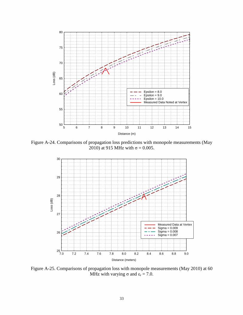
Figure A-24. Comparisons of propagation loss predictions with monopole
measurements (May 2010) at 915 MHz with σ = 0.005. ........................................... 33

viii
Figure A-25. Comparisons of propagation loss with monopole measurements (May
2010) at 60 MHz with varying σ and εr = 7.0. ........................................................... 33
Figure A-26. Comparisons of propagation loss with monopole measurements (May
2010) at 90 MHz with varying σ and εr = 7.0. ........................................................... 34
Figure A-27. Comparisons of propagation loss with monopole measurements (May
2010) at 60 MHz with varying σ and εr = 7.5. ........................................................... 34
Figure A-28. Comparisons of propagation loss with monopole measurements (May
2010) at 60 MHz with varying σ and εr = 8.0. ........................................................... 35
Figure A-29. Comparisons of propagation loss with monopole measurements (May
2010) at 120 MHz with varying σ and εr = 9.0. ......................................................... 35

ix
TABLES
Page
Table 1. Values of permittivity (ε) for the distance range of 8 to 10 meters at
frequencies at and above 150.0 MHz (August 2009 data). ........................................ 16
Table 2. Values of εr for the various distances, frequencies, and permittivity for the
distance range of 8 to 10 meters for frequencies below 150 MHz (August
2009 Data). ................................................................................................................ 17
Table 3. Values of εr at different frequencies at a distance of 8.3 meters (May 2010
data). .......................................................................................................................... 18
Table 4. Values of conductivity and permittivity, for various frequencies for the
single distance of 8.3 meters (May 2010 data). ......................................................... 18


FREE-FIELD MEASUREMENTS OF THE ELECTRICAL PROPERTIES OF SOIL
USING THE SURFACE WAVE PROPAGATION BETWEEN TWO MONOPOLE
ANTENNAS
Nicholas DeMinco, Robert T. Johnk, Paul McKenna,
Chriss A. Hammerschmidt, J. Wayde Allen1
This report describes one of three free-field radio frequency (RF) measurement
systems that are currently being developed by engineers at the Institute for
Telecommunication Sciences (NTIA/ITS). The objective is to provide estimates
of the electrical properties of the ground (permittivity and conductivity) over
which the measurement systems are deployed. This measurement system uses
transmission loss measurements between two monopoles placed close to the
ground at specific separation distances. Soil properties are extracted by comparing
measured data with known analytical models and optimizing the results.
Key words: antenna; radio-wave propagation; deconvolution; Fourier transform; frequency
domain; gating; monopole antenna; reflectivity, signal processing, S-parameters,
time domain; transmission loss; propagation measurement
1 INTRODUCTION
A near-earth propagation measurements program was initiated at the Institute for
Telecommunication Sciences (NTIA/ITS) Table Mountain Field Site (TMFS) in August 2009
under the sponsorship of the Naval Research Laboratory (NRL). A second set of measurements
sponsored by the Table Mountain Research Project were performed in May 2010. The purpose of
these efforts was to develop improved propagation prediction tools and models for close-in
distances (2–250 m) and low antenna heights (0–3 m). While comparing measured and modeled
results, questions arose about the assumed dielectric permittivity and conductivity of the soil at
the TMFS. These ground constants can have a significant influence on RF propagation
predictions near the ground and need to be accurately characterized.
The system described in Section 2 of this report performs two-port transmission measurements
between two resonant ground-plane mounted monopoles placed at various separation distances
ranging from 2 to 250 meters. The measurements were conducted along a main access road at
various road positions using stepped-frequency transmission measurements over the Earth
between the monopoles. For the set of measurements taken in August 2009, the separation
distances were varied within the full range; for the second set of measurements taken in May
2010, the separation distance was fixed at 8.3 meters. It is desirable to locate the antennas as
close to ground as possible, so that the predominant mode of propagation is by means of the
surface wave. The monopoles were placed 8.9 centimeters above ground to simplify feeding the
1 The authors are with the Institute for Telecommunication Sciences, National Telecommunications and Information
Administration, U.S. Department of Commerce, Boulder, CO 80305.

2
antenna from below the ground plane while maintaining the antenna height as close to zero with
respect to a wavelength as possible.
For the frequencies under consideration (30 to 915 MHz), this is essentially equivalent to a zero
height antenna, because the wavelengths are between 0.328 and 10.0 meters. The propagation
between the antennas is predominantly via the Norton surface wave [1]–[3], because the
antennas are very close to the Earth. At this height, the direct and reflected waves cancel each
other, resulting in only the surface wave component of the ground wave as the mechanism for
radio-wave propagation. The skin depth of the propagating wave into the soil is significant, so
the use of the surface wave effectively probes the ground, resulting in an aggregate measure of
the ground constants of the soil. Actual skin depths for different values of sigma (σ) and epsilon
(εr) will be presented in Section 4.

3
2 MONOPOLE TRANSMISSION MEASUREMENT SYSTEM
The system, a schematic of which is shown in Figure 1, uses a vector network analyzer (VNA) to
perform stepped-frequency transmission (S-parameter) measurements over a wide frequency
range between two resonant monopoles separated at a distance d. The monopoles are mounted at
the center of circular aluminum ground planes, and are coaxially fed on the bottom side of the
ground planes. Each antenna is soldered to a coaxial feedthrough that provides a type-N
connection from the bottom. Dielectric spacers on the plates provide enough clearance for a
coaxial cable to feed the monopoles.
The nominal height of the ground planes is h1=h2=8.9 cm. The VNA is configured to perform
stepped-frequency measurements of the S-parameter S21. Measurement data were acquired over a
frequency range from 300 kHz to 6 GHz. Data for the analysis was extracted from this
measurement set over a frequency range subset of 30 MHz to 915 MHz, because of the limited
dynamic range outside the operating frequency range of the resonant monopole antennas.
The system is calibrated by connecting the transmitting and receiving cables together and
performing a through calibration. The cables are then connected to the antennas and the
transmission loss is measured.
VNA
S21
(ground)
Tx
MonopoleRx
Monopole
d
h1 h2
Tx
Port 2
Tx
Port 1
RF Cable RF CableVNAVNA
S21
(ground)
Tx
MonopoleRx
Monopole
d
h1 h2
Tx
Port 2
Tx
Port 1
RF Cable RF Cable
Figure 1. Schematic diagram of the monopole measurement system.
Both magnitude and phase information are acquired, which permits transformations to and from
the time and frequency domain. This capability provides more insight into the propagation over
the ground and permits processing to enhance accuracy and signal fidelity by windowing the
stepped frequency data and time gating the time domain waveform.
A flow chart showing the signal processing sequence is shown in Figure 2. These stepped-
frequency data are windowed to suppress undesired out-of-band effects, then inverse Fourier
transformed to obtain a time-domain waveform. Time gating is then applied to isolate the desired
propagation events and to improve signal-to-noise performance. Finally, the gated waveform is

4
Fourier transformed to yield the gated S21g. Figure 3 depicts the results of this process and shows
the influence on the amplitude spectra when the effects of a nearby reflector are removed using
time gating. The corresponding ungated and gated time domain waveforms are shown in Figure
3(b). The presence of a nearby scatterer manifests itself in the secondary wavelet that follows the
main propagation event. After this packet is gated out and Fourier transformed, the resulting S21
is smoothed out and systematic scalloping is removed. A combination of signal processing and
time gating were used to remove the effects of nearby reflectors and scatters to isolate the
coupling between the antennas. This produces a significant improvement in signal fidelity and
signal-to-noise ratio.
The surface wave loss measurements at the TMFS were performed by measuring the propagation
loss between two matched monopole antennas each mounted on a separate circular ground
planes using techniques described in the previous paragraphs. The ground constants are
determined by using the measured loss of the surface wave between two antennas at known
distances. The antennas were a set of quarter-wave monopoles resonant at 150, 250, 430, 700,
and 915 MHz. The ground planes were approximately one-quarter wavelength in radius. The
antennas were spaced at known separation distances and placed on the ground at a height of
approximately zero meters (8.9 cm) above ground. Practical limitations of feeding the antennas
prevented heights less than 8.9 cm, but analysis has verified that there is a negligible difference
in results between the 8.9 cm and zero antenna heights.
The approach was to compute the propagation losses between the two antennas at the fixed
distances for a variety of ground constants and frequencies and match the measured losses to the
appropriate curves to obtain the various ground constants. The distances between the antennas at
which measurements were taken in 2009 included: 2, 3, 4, 5, 8, 10, 15, 20, 25, 30, 35, 40, 50, 80,
100, 150, 180, 200, and 250 meters. Data for this scenario reflects a road section with a flat
terrain measurement environment. The portion of the path used for performing the measurements
was line-of-sight. The frequency was stepped from 300 kHz to 6000 MHz while the antennas
remained stationary at each of the distances listed above. In 2010, a second set of measurement
data was taken at the same location, but only at a fixed distance of 8.3 meters.

5
Stepped-Frequency
S21(f)
Window (BP Filter)
fhighflow
Inverse Fourier Transform
Time-Domain Waveform
Time Gate
Fourier Transform
S21g(f)
Stepped-Frequency
S21(f)
Stepped-Frequency
S21(f)
Window (BP Filter)
fhighflow
Window (BP Filter)
fhighflow
Inverse Fourier TransformInverse Fourier Transform
Time-Domain WaveformTime-Domain Waveform
Time GateTime Gate
Fourier TransformFourier Transform
S21g(f)S21g(f)
Figure 2. Flowchart of the sequence used to post process the monopole transmission
measurements.
(a)
0 400 800 1200 1600Frequency (MHz)
-140
-120
-100
-80
-60
|S2
1| (d
B)
250 MHz MonopoleS21
S21 time gated
0 20 40 60 80 100Time (ns)
-0.00012
-8E-005
-4E-005
0
4E-005
8E-005
0.00012
s2
1(t
)
desired propagationpacket
spurious reflection
(b)(a)
0 400 800 1200 1600Frequency (MHz)
-140
-120
-100
-80
-60
|S2
1| (d
B)
250 MHz MonopoleS21
S21 time gated
0 20 40 60 80 100Time (ns)
-0.00012
-8E-005
-4E-005
0
4E-005
8E-005
0.00012
s2
1(t
)
desired propagationpacket
spurious reflection
(b)
Figure 3. (a) Ungated and time-gated (0–36 ns) amplitude spectra for 700 MHz resonant
monopoles separated at d = 8 m. (b) Corresponding gated and ungated time-domain waveforms.
6
3 GROUND-WAVE PROPAGATION COMPUTATION METHOD AND THE
DEVELOPMENT OF THE UNDISTURBED-FIELD MODEL
The ground wave includes the direct line-of-sight space wave, the ground-reflected wave, and
the Norton surface wave that propagates along the Earth. The Norton surface wave will hereafter
be referred to as a surface wave in this report. Propagation of the ground wave depends on the
relative geometry of the transmitter and receiver locations and antenna heights. The radio wave
propagates primarily as a surface wave when both the transmitter and receiver antennas are close
to the Earth (approximately 0.25 wavelength or less), because the direct and ground-reflected
waves in the space wave components of the ground wave cancel each other out. As a result, the
surface wave is the only wave component that continues to propagate.
This cancellation occurs because the elevation angle is zero, the two waves (direct and reflected)
are equal amplitude and opposite in phase, and they travel the same distance. The surface wave is
predominantly vertically polarized, since the ground conductivity effectively attenuates most of
the horizontal electric field component at a rate many times that for the vertical component of the
electric field. When one or both antennas are elevated above the ground to a significant height
with respect to a wavelength (greater than 0.25 wavelength), the space wave predominates.
When the antennas are close to the ground with respect to a wavelength, the surface wave
propagates along and is guided by the Earth’s surface. This is similar to the way that an
electromagnetic wave is guided along a transmission line. The attenuation of this wave is directly
affected by the ground constants of the Earth along which it travels [1]. Charges induced in the
Earth by the surface wave travel with the surface wave and create a current in the Earth. The
Earth carrying this current can be modeled as a leaky capacitor ( a capacitive reactance shunted
by a resistance). The characteristics of the Earth as a conductor are therefore represented by this
equivalent parallel resistor-capacitor circuit. The Earth’s conductivity acts as a resistor and the
Earth’s dielectric constant acts as a capacitor. As the surface wave passes over the surface of the
Earth, it is attenuated due to the current flowing through the Earth’s resistance. Energy is taken
from the surface wave to supply the losses in the ground.
Since the equivalent circuit of the Earth is a resistor of resistance R (ohms) and capacitor of
capacitance C (Farads) in parallel, more current flows through the resistance at lower
frequencies, R<<1/ωC (ω = 2πf where f is the frequency in Hertz); and the attenuation factor is
then primarily dependent on the conductivity of the Earth and the frequency. At lower HF
frequencies, AM broadcast (medium frequencies), and lower frequencies in the LF band (below
300 kHz), the Earth can be regarded as being purely resistive in nature. For frequencies above
about 150 MHz, the impedance represented by the Earth is primarily capacitive, so the
attenuation factor for the surface wave at a given physical distance is determined by the
dielectric constant of the Earth and the frequency [1]. The impedance of the capacitor decreases
with increasing frequency.
The ITS Undisturbed-Field Model was originally developed for very short-range propagation for
distances of 2 to 30 meters. Subsequently, the model was shown to be accurate for flat terrain up
to 2 kilometers [2]. The minimum distance is based on staying at distances greater than the
distance within which the reactive field of the antenna is present. This is a distance of one
wavelength. Extensive testing with exact models at close-in distances has verified the

7
computation accuracy for distances as close as 2 meters over the 150 MHz to 6000 MHz
frequency band [2].
This method involves the calculation of the undisturbed electric field as a function of antenna
heights, distance, frequency, and the ground constants from which the path loss is derived. The
undisturbed field is that electric field produced by a transmitting antenna at different distances
and heights above ground without any field-disturbing factors such as other receiver antennas in
the proximity of the receiver antenna location. The undisturbed electric field technique includes
near-field effects of the transmit antenna, the complex two-ray model, antenna near-field and far-
field response, and the surface wave. Since this is a line-of-sight model, the ground is assumed to
be flat over the distance of 2 kilometers or less with no irregular terrain present. For distances of
less than 5 kilometers, the curvature of the Earth has a negligible effect and can be assumed to be
flat for frequencies less than 6 GHz over a smooth Earth [3]. The model was originally
developed for antenna heights of 1 to 3 meters, but further improvements in the model have
demonstrated that the model can be used for antenna height ranges from 0 to 1 meter. It is valid
for frequencies from 150 MHz to 6000 MHz [2].
The space wave component (direct and reflected waves) and surface wave component of the ITS
Undisturbed-Field Model are based on the Sommerfeld integral arising from the solution for the
field due to an elemental dipole above a uniform, finitely-conducting, dielectric half space [4]–
[6]. The half space is bounded by the Earth-air interface. Norton [4], [5], in his effort to simplify
the expressions developed by Sommerfeld [7], derived equations that clearly show the surface
wave and space wave components. Jordan [8] simplified Norton’s equations by deleting the
higher order terms for the vertical and radial directed components of the electric field in
cylindrical coordinates. These higher order terms represent the induction and near field of the
antenna and diminish rapidly with distance. Jordan [8] further reduced the equation complexity
by combining the vector equations for the vertical and radial directed field components, and then
separating the resulting equation into a total space (direct and reflected waves) and surface wave
components. At distances within the line of sight, the field strength of the space and the surface
wave for vertical polarization is given by [4], [5] and [8]:
cos3021
21
r
eR
r
eIkLiE
ikr
v
ikr
space
(1)
2
22
2 2 2
2
sin30 1 1 2 cos 1
2
ikr
surface v
eE i IkL R A u u
r
, (2)
where:
k = 2π/λ,
A is the flat-Earth attenuation function,
I is the peak dipole current amplitude in amperes,
L is the length of the dipole in meters,
u2 = (εr-iσ/ωε0)
-1,
ω is the angular frequency and is equal to 2πf,

8
f is the radio frequency in Hertz,
μ is the magnetic permeability of the Earth, μ = μr ·4π·10-7
henries per meter,
μr is the relative permeability of the Earth,
ε =εr·ε0= εr·8.85·10-12
= the permittivity of the Earth in Farads per meter,
εr is the relative permittivity of the Earth,
ε0 is the permittivity of free space in Farads per meter,
σ is the conductivity of the Earth in Siemens per meter,
is the angle representing the direction of the incident wave measured with respect to
the Earth’s surface,
h1 is the height of the transmitter antenna in meters,
h2 is the height of the receiver antenna in meters,
d is the horizontal distance along the Earth.
The distance 21
2
21
2
1 hhdr is the distance between the dipole and the observation point
in meters.
The distance 1
2 22
2 1 2r d h h is the distance between the dipole image and the observation
point in meters.
Rv is the complex reflection coefficient for vertical polarization and is given by:
2
00
2
00
cossin
cossin
ii
ii
R
rr
rr
v
(3)
Equations (1) through (3) are different for horizontal polarization and can be found in [8].
The attenuation function, A, is the ratio of the electric field from a short vertical dipole over the
lossy Earth’s surface to that field from the same short vertical dipole located on a flat perfectly
conducting surface, and takes into account the ground losses. There are two forms of the
attenuation function presented in this report. The ITS Undisturbed Field Model was developed in
several versions, with each version improving on the previous versions. In response to a request
from the NTIA Office of Spectrum Management, model development was initiated to
specifically address the application of propagation loss predictions for very low antenna heights
and close-in distances [2].
The original concept for development of a propagation model [2] used the Numerical
Electromagnetic Code (NEC) software [12], which uses a method of moments technique in
electromagnetics to compute the electric field versus frequency, ground constants, antenna
heights, and distances. This electric field is then converted to a basic transmission loss as
described in [2]. This original method was cumbersome and required running the NEC software

9
many times to get results over a variety of input parameters and scenarios to create lookup tables
to cover the various parameter ranges. This was Version 0 of the ITS Undisturbed-Field Model.
Version 0 needed to be streamlined into a more efficient and flexible computation method in the
form of a computer model that would rapidly compute propagation loss to be used in system
performance computations and other analysis applications. In response to a Naval Research
Laboratory request to further develop the initial concept into a fast efficient computation model,
Version 1 was developed. The approximate attenuation function described by (4) and (5) is used
in Version 1 of the Undisturbed-Field Model which is described in this section. It uses simple
algebraic equations to perform the calculations. Version 2 uses the more exact representation of
the attenuation function and is valid for a wider variety of parameters than Version 1. It uses a
more complex mathematical algorithm to perform its computations when compared to the simple
equations of Version 1. Version 2 contains the more precise form of the attenuation function that
is used in the ITS Undisturbed-Field Model to perform the propagation loss computation in this
analysis.
Version 1 of the ITS Undisturbed Field Model uses the original Norton approximation to the
attenuation function. Norton simplified the exact and more complex equations for the surface
wave attenuation function into two forms that are more amenable to calculation. Version 1 with
the Norton approximations to the flat-Earth attenuation [4], [5] function of the surface wave can
be easily implemented on a programmable calculator and is reasonably accurate for line-of-sight
propagation [6].
The Version 1 attenuation function, A, is given by:
for p0 < 4.5 and all b:
2 0
0 0
5
0.43 0.01 0 8sin2
pp p p
A e b e
(4a)
for p0 > 4.5 and all b:
0
5
0 8
0
1sin
2 3.7 2
ppA b e
p
, (4b)
where for vertical polarization:
2
0 22
1
3
cos
54 10
1tan
18 10
r
R km f MHz bp
x
f MHzb
x
(5a)

10
and for horizontal polarization:
4
0
1
3
6 10
cos
1tan
18 10
r
R km xp
b
f MHzb
x
, (5b)
where:
3
2 10R km r is the distance between the observation point and the dipole image in
km,
σ is the conductivity of the Earth in Siemens per meter,
εr is the relative permittivity of the Earth,
f(MHz) is the frequency in MHz.
These results are approximations. More exact results were sought for implementation in the ITS
Undisturbed-Field Model.
Version 2 uses Norton’s more exact mathematical algorithm to compute the attenuation function
for the more precise approximations ((6) and (7)) to the flat-Earth attenuation function. It is
accurate for a wider range of parameters, but is more difficult to implement. This was derived by
Norton from the original Sommerfeld formulation [7] for the flat-Earth attenuation function of
the vertically polarized surface wave [5] and is given by:
1
1 11p
A i p e erfc i p , (6)
where
2 22 21 0
2
i bk rp i p e
(7a)
rNN
cos11
(7b)
12
1
2 0
r
kN i
k
(7c)
1 0
2 0 0
rk i
k
(7d)
21
2
21
2
2 hhdr (7e)
11
1 2
2
cos .r
h h
r
(7f)
The horizontal component of the surface wave attenuates at a rate several orders of magnitude
greater than the vertical component and has a magnitude that is negligible in comparison to the
vertically polarized component of the surface wave [8].
Equations (6) and (7) are implemented in Version 2 of the ITS Undisturbed-Field Model used for
computation of the propagation losses. The complementary error function, designated by erfc in
(6), is described in [9]. The parameters p0 and b are as defined above (see (5a) and (5b)), and
1i .
The field strength at small distances is directly proportional to the square root of the power
radiated by the transmitter and the directivity of the antenna in the horizontal and vertical planes.
If the antenna is non-directional in the horizontal plane and has a vertical directional pattern that
is proportional to the cosine of the elevation angle (this corresponds to a short vertical antenna),
then the electric field at one kilometer for an effective radiated power of one kilowatt is 300
mV/m [1]. The flat-Earth attenuation function, A, depends on frequency, distance, and the
ground constants of the Earth along which the wave is traveling. A numerical distance, p0, and
phase angle, b, can be computed and are functions of frequency, ground constants, and distance
in wavelengths.
If the numerical distance, p0, is less than one, then the attenuation function is very close to one,
and, as a result, for distances close to the transmitting antenna the losses in the Earth have very
little effect on the electric-field strength of the surface wave. In this region, the electric field
strength is inversely proportional to distance. For situations where the numerical distance
becomes greater than unity, the attenuation function rapidly decreases in magnitude. When the
numerical distance becomes greater than 10, the attenuation factor is also inversely proportional
to distance. In this circumstance, the combination of the attenuation factor and the un-attenuated
electric field being inversely proportional to distance results in the electric field strength of the
surface wave being inversely proportional to the square of the distance.

12
4 ELECTRIC FIELD PENETRATION DEPTH OF THE SOIL AND ITS EFFECT ON
GROUND-WAVE PROPAGATION
The depth to which the ground currents and electric field penetrate below the Earth’s surface and
still maintain an appreciable magnitude is determined by the average values of the Earth
conductivity (σ) and relative permittivity (εr), and the frequency. Penetration depth is similar to a
skin depth phenomenon in a good conductor, but the Earth is a poor conductor. The skin depth
ranges from a fraction of a meter at the highest frequencies for VHF communications to tens of
meters at AM broadcast and lower frequencies. For this reason, ground-wave propagation at the
lower frequencies is not particularly dependent on properties at the actual ground surface.
Therefore, a recent rainfall which would result in a dramatic change of permittivity at the ground
surface would not significantly affect propagation at MF and LF frequencies. However, at VHF
frequencies a recent rainfall could affect the propagation of radio waves due to the additional
moisture content of the ground near the ground surface.
The electric field strength at a distance z below the surface of the Earth is given by [10]:
0 ,zE E e (8)
where:
E0 is the electric field intensity at the surface of the Earth,
z is the depth in meters below the surface of the Earth,
α is the attenuation per meter of the electric field intensity
The attenuation per meter α is given by:
21 1
1 ,2 2
(9)
where:
ω is the angular frequency and is equal to 2πf,
f is radio frequency in Hertz,
μ is the magnetic permeability of the Earth μ = μr · 4π x 10-7
Henries per meter,
μr is the relative permeability,
ε = the permittivity of the Earth = εr · (8.85 x 10⁻¹²
) Farads per meter,
εr is the relative permittivity of the Earth,
σ is the conductivity of the Earth in Siemens per meter.

13
The distance the wave must travel in a lossy medium to reduce its amplitude to e-1
=0.368 of its
value at the surface is δ = 1/α meters and is called the skin depth of the lossy medium. For other
values of attenuation of the electric field, r=e-αz
, one can use α to determine the distance z below
the surface where the electric field is attenuated to that ratio r. The ratio r is always less than or
equal to 1. The distance z is given by:
ln r
z - ,
(10)
where lnr is the natural logarithm of r.
An example is where f=300 kHz, μr = 1 for a nonmagnetic Earth, εr = 15 for average ground, σ =
.005 for average ground. The attenuation α is calculated as .0751 per meter and δ is calculated as
1/α = 13.32 meters.
The skin depth is the distance at which the electric field is e-1
or .368 (36.8 percent) of its value
at the surface of the Earth [10]. The electric field at this large percentage does not represent a
significant attenuation of the electric field. Some applications may require a lower electric field
percentage such as 10 percent. If the distance, z, at which the electric field is .1 (10 percent) of its
value at the surface is desired, then ln r is ln (.1) = -2.3026, and α = .0751, so
2 3026 30 66z . / . meters. Figure 4 shows the skin depth of several types of media as a
function of frequency. The skin depth does not vary by significant amounts for each media type
at these frequencies. Figure 4 demonstrates how significant the different ground constants are in
affecting the magnitude of the skin depth. It shows that the skin depth is quite large for poor and
average ground. Figure 5 is an expansion of Figure 4 along the frequency axis to show the skin
depth in the 100 kHz to 10 MHz range, and demonstrates how large the skin depths are below
2 MHz.

14
0
2.5
5.0
7.5
10.0
12.5
01x10
32x10
33x10
34x10
35x10
36x10
3
Sigma = 5.0, Epsilon = 81.0 Sea WaterSigma = 0.010, Epsilon = 81.0 Fresh WaterSigma = 0.020, Epsilon = 25.0 Good GroundSigma = 0.005, Epsilon = 15.0, Average GroundSigma = 0.005, Epsilon = 6.0 Less Than Average GroundSigma = 0.001, Epsilon = 4.0 Poor Ground
Frequency (MHz)
Skin
De
pth
(m
)
Skin Depth for 1/e E-Field Attenuation Versus Frequency With Media Type as Parameter
Figure 4. Skin depth for 1/e E-field attenuation versus frequency for various media types.
0
10
20
30
40
0 2 4 6 8 10
= 5.0, r = 81.0 Sea Water
= 0.010, r = 81.0 Fresh Water
= 0.020, r = 25.0 Good Ground
= 0.005, r = 6.0 Less Than Average Ground
= 0.005, r = 15.0 Average Ground
= 0.001, r = 4.0 Poor Ground
Frequency (MHz)
Skin
De
pth
(m
ete
rs)
Figure 5. Skin depth for 1/e E-field attenuation versus frequency for various media types for
lower frequencies.

15
4.1 Computed Sensitivity of Propagation Loss to Values of Epsilon (εr) and Sigma (σ)
The Undisturbed-Field Model [2] developed at ITS was used to perform all propagation loss
prediction computations as a function of antenna heights, relative dielectric constant (εr) ,
conductivity (σ), frequency, and distance. The results of these computations are shown in the
figures in Appendix A. The model has been verified with comparisons to more exact models [2]
and measured data.
Figure A-1 shows the propagation loss for three types of ground for a distance of 10 meters for
antenna heights at zero meters. There is a significant difference in the predicted propagation loss
between poor (εr = 4.0, σ = 0.001) and good ground (εr = 25.0, σ = 0.020). As part of this
analysis effort, a study was performed to determine the sensitivity of the propagation loss to
variations in conductivity (σ) and relative permittivity (εr). Figures A-2 through A-5 show the
sensitivity of propagation loss to σ and εr for a separation distance of 10 meters. The heights of
the transmitter and receiver antennas for all figures in the Appendix are equal to zero. The
computations and measurements are based on heights of 8.9 centimeters which is equivalent to a
zero height at these frequencies. Computations at heights of 8.9 centimeters and 0.0 centimeters
verify this assumption. Figure A-2 shows that for a low conductivity, the loss is very dependent
on the value of εr, but Figure A-3 shows that for a higher σ the loss has less dependence on εr,
particularly for frequencies at and below 150 MHz. Figures A-4 and A-5 show that the loss is
dependent on σ only for frequencies at and below 150 MHz. The sensitivity to variation in σ is
greater for lower values of εr. Figure A-4 has a value of εr = 4 and a higher sensitivity to changes
in σ, whereas Figure A-5 has a value of ε r = 25 and a much lower sensitivity to variations in σ.
Figure A-6 is a plot of loss versus σ with an expanded scale and shows how insensitive the loss
is to variations in σ for frequencies above 150 MHz. Figure A-6 shows that there is some
capability to determine σ from lower frequency data at and below 150 MHz.

16
5 SOIL DIELECTRIC PROPERTIES OBTAINED AT TABLE MOUNTAIN USING
MONOPOLE TRANSMISSION MEASUREMENTS
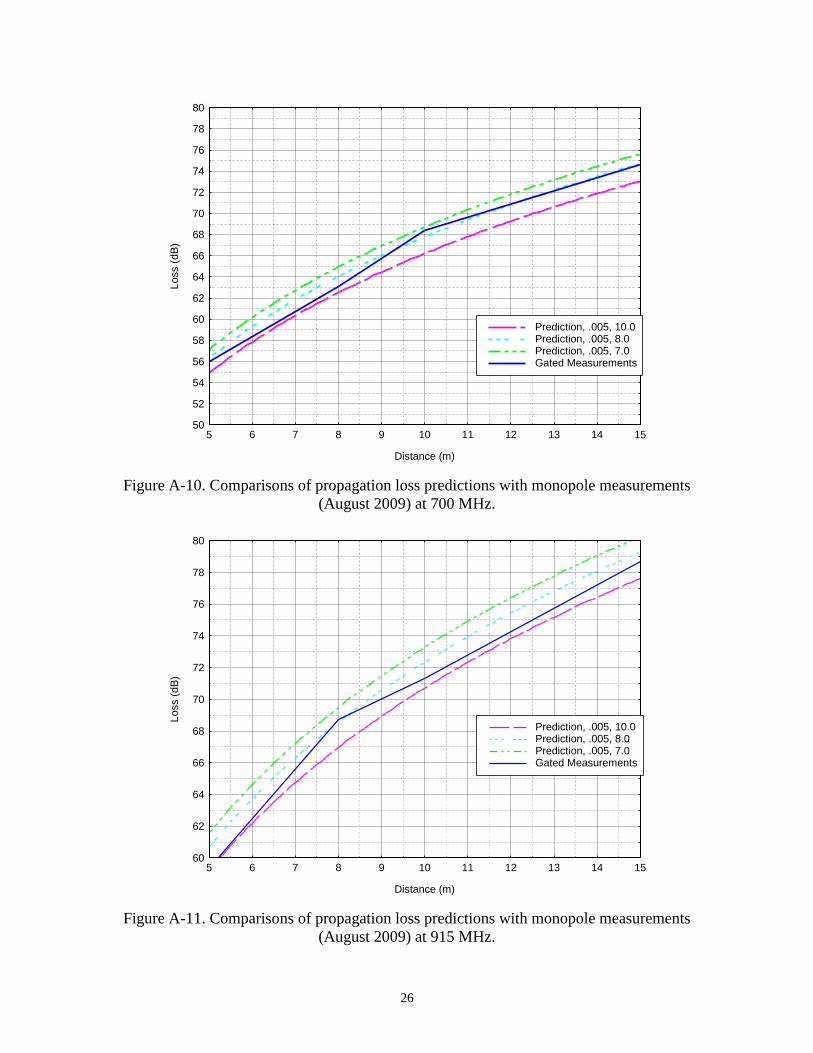
Figures A-7 through A-11 show the results of comparing predictions to measurements for data
taken in late August of 2009. The distance and vertical scales were expanded for better vertical
scale resolution. Measured data was originally recorded over separation distances ranging from 2
to 250 meters using monopole antenna pairs resonant at the five frequencies (150.5, 250, 430,
700 and 915 MHz). The data show that the dielectric constants vary over the distance of the
measurement path. Most data analysis took place over shorter distances. This study concentrated
on distances in the 5 to 15 meter range. The ground at Table Mountain is not homogeneous,
which accounts for the erratic variation of loss versus distance shown in Figures A-7 through A-
11.
These data were available to determine the ground parameters of σ and εr for the measured data
collected in August 2009. Since the values of σ could not be determined at the frequencies above
150 MHz as discussed in Section 3.1, only εr was obtained from these plots. This is due to the
lack of sensitivity of the propagation loss at or above 150 MHz to values of σ. At lower
frequencies below 150 MHz, the loss is insensitive to variations in εr, but sensitive to variations
in σ. The permittivity varies as a function of distance and frequency. Table 1 shows the results of
extracting the values of permittivity from Figures A-7 through A-11 (August 2009 data) for a
conductivity of σ = 0.005 Siemens per meter. Table 2 shows the values of σ from Figures A-12
through A-19 (August 2009 data). The average value of εr in Table 1 is approximately 6.0 for the
first three values of Table 1 and 7.0 for the entire table, so the values of εr of 6.0 to 7.0 were used
to determine σ, because εr is known to be relatively constant in the 30 to 150 MHz region [11].
Referring to Figures A-2 and A-3 the loss versus εr curves are relatively flat between εr = 6.0 and
7.0 for frequencies less than 150 MHz.
Table 1. Values of permittivity (ε) for the distance range of 8 to 10 meters at frequencies at and
above 150.0 MHz (August 2009 data).
Frequency (MHz) Permittivity, εr Conductivity, σ (S/m)
150.5 7.0 to 8.0 0.005
250.0 6.0 to 7.0 0.005
430.0 4.0 to 5.0 0.005
700.0 7.0 to 9.0 0.005
915.0 8.0 to 9.0 0.005
The analysis using the lower frequencies below 150 MHz was performed to determine σ by
compensating the measured data to take into account the reduced efficiency of the antennas when
operating below 150 MHz and then comparing these measured data to the predictions at these
lower frequencies. The distance range was reduced to 7 to 9 meters to allow expansion of the
vertical scales for better resolution.

17
Using data at lower frequencies below 150 MHz, this compensation technique was used to
extract σ, from the measured data shown in Figures A-12 to A-19. The monopole antennas are
narrowband and resonant at their design frequencies. The raw measured data shows the maximal
response of these antennas at their resonant frequencies. The compensation technique included a
correction by applying an impedance mismatch loss in addition to an adjustment of average gain
at the lower frequencies.
This mismatch and gain compensation information was obtained by modeling the 150 MHz
monopole antennas at frequencies below 150 MHz using the method of moments technique of
the NEC software [12]. The NEC software can compute an antenna’s radiation pattern, gain, and
input impedance characteristics. The physical and electrical structure of the 150 MHz resonant
monopole on a circular ground plane was used as input to the NEC software. When this antenna
is analyzed at frequencies other than 150 MHz with the NEC software, the gain, input
impedance, and radiation pattern are computed at the other frequencies computed.
The mismatch loss was computed from the computed input impedance using conventional
techniques as found in [8]. The total degradation in gain and efficiency at frequencies below 150
MHz was obtained by adding the gain degradation and the impedance mismatch loss. Using the
150 MHz monopole provided useful data down to 30 MHz. The results from Figures A-12
through A-19 are summarized in Table 2 for the frequencies listed.
Table 2. Values of εr for the various distances, frequencies, and permittivity for the distance
range of 8 to 10 meters for frequencies below 150 MHz (August 2009 Data).
Frequency (MHz) Permittivity, εr Conductivity, σ (S/m)
30.0 6.0 0.005
60.0 6.0 0.009
30.0 6.5 0.005
60.0 6.5 0.007
30.0 6.7 0.004
60.0 7.0 0.007
30.0 7.0 0.004
60.0 7.0 0.006
A second set of measured data was recorded in May 2010 using the same stepped frequency
technique using sets of monopole antennas resonant at 150.5, 250, 430, 700, and 915 MHz, but
only at a single distance of 8.3 meters. A limited amount of data was available from these
measurements. It was determined that the relative permittivity (εr) and conductivity (σ) were
higher for this set of measurements. The results of these May 2010 measurements are shown in
Figures A-20 through A-24, which are expanded plots for better resolution. These figures were
used to determine εr of the ground at and above 150 MHz. Table 3 summarizes the values of εr
extracted from Figures A-20 through A-24 for σ = 0.005 Siemens/meter.

18
Table 3. Values of εr at different frequencies at a distance of 8.3 meters (May 2010 data).
Frequency (MHz) Permittivity, εr Conductivity, σ (S/m)
150.5 9.0 to 10.0 0.005
250.0 10.0 0.005
430.0 7.5 0.005
700.0 9.0 0.005
915.0 9.0 0.005
These values of εr from Figures A-20 through A-24 were used to determine the conductivity in
Figures A-25 through A-29 at frequencies below 150 MHz.
The higher values for εr of the May 2010 data when compared to measurements of the previous
year (August 2009) were thought to be a result of increased moisture content due to the heavier
rainfall that occurred prior to the May 2010 measurements. Soil conditions were drier when the
previous measurements were taken, in August 2009. For both sets of measurements the ground
was not homogeneous, but this surface wave technique of determining the ground constants
results in an aggregate measure of the non-homogeneous ground at Table Mountain.
Figures A-25 through A-29 present the results of comparing the May 2010 measured data to the
predictions, with plots expanded for better resolution. These figures were used to determine σ of
the ground for the second set of measurements using the lower frequency compensation
technique described previously at frequencies below 150 MHz, since σ could not be resolved
from the measurements above 150 MHz. The plots in these Figures are expanded with better
vertical scale resolution to facilitate the extraction of data. Table 4 summarizes the results of
extracting the values of σ from Figures A-25 through A-29. Referring to Figures A-2 and A-3 the
loss versus εr curves are relatively insensitive to changes in εr between εr = 7.0 to 9.0, which were
the εr values used in Table 4 for determining σ.
Table 4. Values of conductivity and permittivity, for various frequencies for the single distance
of 8.3 meters (May 2010 data).
Frequency (MHz) Permittivity, εr Conductivity, σ (S/m)
30.0 7.0 0.008
30.0 7.5 0.006
30.0 8.0 0.005
90.0 7.0 0.005
120.0 9.0 0.007

19
6 CONCLUSION
It was determined that the propagation loss of the surface wave is relatively insensitive to σ (the
conductivity), but does show significant variation with respect to εr (the relative dielectric
constant) for frequencies including and above about 150 MHz. Lower frequencies below 150
MHz do show some variation with σ, and small variations at these lower frequencies can be used
to determine σ. At higher frequencies, the variation of propagation loss could not be used to
determine σ. This method can be used as a comparison to a vertical incidence (reflection
coefficient) measurement/analysis effort that is currently underway, and could provide possible
verification of values of εr obtained with the vertical incidence method.
Future work would include examining these data above and below 150 MHz using a computer
program with an optimization algorithm to determine the values of εr and σ. Another area of
future work would include developing a method that would use the phase angle of the transfer
function S21 from the measured data with a propagation loss prediction algorithm that contains
phase angle as an alternative method of obtaining the σ from data at frequencies above and
below 150 MHz. Separation of the transfer function into real and imaginary components could
provide better resolution for determination of the σ for comparison to the mathematical
expressions for propagation loss of the surface wave.

20
7 REFERENCES
[1] F.E Terman, Electronic and Radio Engineering, New York: McGraw-Hill Book Co., 1955,
pp.803–808.
[2] N. DeMinco, “Propagation loss prediction considerations for close-in distances and low-
antenna height applications,” NTIA Report TR-07-449, July 2007.
[3] A. Picquenard, Radio-Wave Propagation, New York: John Wiley& Sons, 1974, p.80.
[4] K.A. Norton, “The calculation of ground-wave field intensity over a finitely conducting
spherical Earth,” Proceedings of the Institute of Radio Engineers, Vol. 29, No. 12,
December 1941, pp 623–639.
[5] K.A. Norton, “The propagation of radio waves over the surface of the Earth and in the
upper atmosphere,” Part I, Proc. IRE, Vol. 24, Oct. 1936, pp 1367–1387; Part II, Proc.
IRE, Vol. 25, Sept. 1937, pp. 1203–1236.
[6] R. Li. “The accuracy of Norton’s empirical approximations for ground-wave attenuation,”
IEEE Trans. Ant. Prop., AP-31, No. 4, pp. 624-628, July 1983.
[7] A. Sommerfeld, “Propagation of waves in wireless telegraphy,” Ann. D. Phys. 28, pp.665-
736, March 1909.
[8] E.C. Jordan, Electromagnetic Waves and Radiating Systems, New Jersey: Prentice Hall,
1968, pp.628–650.
[9] M. Abramowitz and I.A. Stegun, Handbook of Mathematical Functions, National Bureau
of Standards AMS 55, U.S. Government Printing Office: Washington, D.C., June 1964, pp.
297–329.
[10] C.A. Balanis, Advanced Engineering Electromagnetics, New York: John Wiley and Sons,
1989, pp.145–154.
[11] International Telecommunications Union (ITU-R), “Electrical characteristics of the surface
of the Earth,” ITU-R Recommendation P.527-3, 1992.
[12] G.J. Burke, “Numerical Electromagnetics Code- NEC-4, method of moments Parts I and
II,” University of California Lawrence Livermore Laboratory Report UCRL-MA-109338,
Livermore, California, 1983.

21
APPENDIX A FIGURES SHOWING RESULTS OF COMPUTATIONS AND
MEASUREMENTS FOR DIELECTRIC CONSTANT AND CONDUCTIVITY
DETERMINATION WITH ALL ANTENNA HEIGHTS EQUAL TO ZERO
0
25
50
75
100
125
0 500 1000 1500 2000 2500 3000 3500 4000 4500 5000 5500 6000
Good Ground: Sigma = 0.020, Epsilon = 25.0Average Ground: Sigma = 0.005, Epsilon = 15.0Poor Ground: Sigma = 0.001, Epsilon = 4.0
Frequency (MHz)
Lo
ss (
dB
)
Loss Versus Frequency for Three Types of Ground
Figure A-1. Propagation loss versus frequency for three types of ground for a distance of 10
meters.

22
20
30
40
50
60
70
80
90
100
110
120
0 5 10 15 20 25
Frequency = 5750 MHzFrequency = 2260 MHzFrequency = 915 MHzFrequency = 430 MHzFrequency = 150 MHzFrequency = 90 MHzFrequency = 60 MHzFrequency = 30 MHz
Epsilon
Lo
ss (
dB
)
Figure A-2. Propagation loss versus epsilon for sigma = 0.001 and distance = 10.0 meters with
frequency as a parameter.
20
30
40
50
60
70
80
90
100
110
120
0 5 10 15 20 25
Frequency = 5750 MHzFrequency = 2260 MHzFrequency = 915 MHzFrequency = 430 MHzFrequency = 150 MHzFrequency = 90 MHzFrequency = 60 MHzFrequency = 30 MHz
Epsilon
Lo
ss (
dB
)
Figure A-3. Propagation loss versus epsilon for sigma 0.020 and distance = 10.0 meters with
frequency as a parameter.

23
20
30
40
50
60
70
80
90
100
110
120
0 0.005 0.010 0.015 0.020
Frequency = 5750 MHzFrequency = 2260 MHzFrequency = 915 MHzFrequency = 430 MHzFrequency = 150 MHzFrequency = 90 MHzFrequency = 60 MHzFrequency = 30 MHz
Sigma (Siemens per meter)
Lo
ss (
dB
)
Figure A-4. Propagation loss versus sigma for epsilon = 4.0 and distance = 10.0 meters with
frequency as a parameter.
20
30
40
50
60
70
80
90
100
110
120
0 0.005 0.010 0.015 0.020
Frequency = 5750 MHzFrequency = 2260 MHzFrequency = 915 MHzFrequency = 430 MHzFrequency = 150 MHzFerquency = 90 MHzFrequency = 60 MHzFrequency = 30 MHz
Sigma (Siemens per meter)
Lo
ss (
dB
)
Figure A-5. Propagation loss versus sigma for epsilon = 25.0 and distance = 10.0 meters with
frequency as a parameter.

24
20
30
40
50
60
70
0 50 100 150 200 250 300 350 400 450 500
Sigma = 0.020 Siemens per meterSigma = 0.010 Siemens per meterSigma = 0.003 Siemens per meterSigma = 0.001 Siemens per meter
Frequency (MHz)
Lo
ss (
dB
)
Loss Versus Frequency for Epsilon = 4.0 With Sigma as Parameter for d = 10.0mh
1 = 0.0 m h
2 =0.0 m Sigma varies from 0.001 to 0.020 with all curves merging together
Figure A-6. Propagation loss versus frequency for epsilon = 4.0 with sigma as a parameter for a
distance of 10 meters with all curves merging together.
30
32
34
36
38
40
42
44
46
48
50
5 6 7 8 9 10 11 12 13 14 15
Prediction, .005, 8.0Prediction, .005, 7.0Predictions, .005, 6.0Gated Measurements
Distance (m)
Lo
ss (
dB
)
Figure A-7. Comparisons of propagation loss predictions with monopole measurements (August
2009) at 150.5 MHz.

25
30
32
34
36
38
40
42
44
46
48
50
52
54
56
58
60
5 6 7 8 9 10 11 12 13 14 15
Prediction, .005, 7.0Prediction, .005, 5.0Predictions, .005 , 6.0Gated Measurements
Distance (m)
Lo
ss (
dB
)
Figure A-8. Comparisons of propagation loss predictions with monopole measurements (August
2009) taken at 250 MHz.
40
42
44
46
48
50
52
54
56
58
60
62
64
66
68
70
5 6 7 8 9 10 11 12 13 14 15
Prediction, .005, 4.0Prediction, .005, 5.0Predictions, .005, 6.0Gated Measurements
Distance (m)
Lo
ss (
dB
)
Figure A-9. Comparisons of propagation loss predictions with monopole measurements (August
2009) taken at 430 MHz.
26
50
52
54
56
58
60
62
64
66
68
70
72
74
76
78
80
5 6 7 8 9 10 11 12 13 14 15
Prediction, .005, 10.0Prediction, .005, 8.0Prediction, .005, 7.0Gated Measurements
Distance (m)
Lo
ss (
dB
)
Figure A-10. Comparisons of propagation loss predictions with monopole measurements
(August 2009) at 700 MHz.
60
62
64
66
68
70
72
74
76
78
80
5 6 7 8 9 10 11 12 13 14 15
Prediction, .005, 10.0Prediction, .005, 8.0Prediction, .005, 7.0Gated Measurements
Distance (m)
Lo
ss (
dB
)
Figure A-11. Comparisons of propagation loss predictions with monopole measurements
(August 2009) at 915 MHz.

27
15
16
17
18
19
20
21
7.0 7.2 7.4 7.6 7.8 8.0 8.2 8.4 8.6 8.8 9.0
Sigma = 0.005Sigma = 0.004Sigma = 0.003Corrected Measured Data
Distance (meters)
Lo
ss (
dB
)
Figure A-12. Corrected measured propagation loss data (August 2009) versus distance compared
to predicted loss for 30 MHz with εr = 6.0 and σ as a parameter.
25
26
27
28
29
30
7.0 7.2 7.4 7.6 7.8 8.0 8.2 8.4 8.6 8.8 9.0
Sigma = 0.010Sigma = 0.009Sigma = 0.008Sigma = 0.007Corrected Measured Data
Distance (meters)
Lo
ss (
dB
)
Figure A-13. Corrected measured propagation loss data (August 2009) versus distance compared
to predicted loss for 60 MHz with εr = 6.0 and σ as a parameter.

28
15
16
17
18
19
20
7.0 7.2 7.4 7.6 7.8 8.0 8.2 8.4 8.6 8.8 9.0
Corrected Measured DataSigma = 0.005Sigma = 0.004Sigma = 0.003
Distance (meters)
Lo
ss (
dB
)
Figure A-14. Corrected measured propagation loss data (August 2009) versus distance compared
to predicted loss for 30 MHz with εr = 7.0 and σ as a parameter.
25
26
27
28
29
30
7.0 7.2 7.4 7.6 7.8 8.0 8.2 8.4 8.6 8.8 9.0
Corrected Measured DataSigma = 0.007Sigma = 0.006Sigma = 0.005Sigma = 0.004
Distance (meters)
Lo
ss (
dB
)
Figure A-15. Corrected measured propagation loss data (August 2009) versus distance compared
to predicted loss for 60 MHz with εr = 7.0 and σ as a parameter.

29
15
16
17
18
19
20
7.0 7.2 7.4 7.6 7.8 8.0 8.2 8.4 8.6 8.8 9.0
Sigma = 0.005Sigma = 0.004Sigma = 0.003Corrected Measured Data
Distance (meters)
Lo
ss (
dB
)
Figure A-16.Corrected measured propagation loss data (August 2009) versus distance compared
to predicted loss for 30 MHz with εr = 6.5 and σ as a parameter.
25
26
27
28
29
30
7.0 7.2 7.4 7.6 7.8 8.0 8.2 8.4 8.6 8.8 9.0
Sigma = 0.009Sigma = 0.008Sigma = 0.007Sigma = 0.006Corrected Measured Data
Distance (meters)
Lo
ss (
dB
)
Figure A-17. Corrected measured propagation loss data (August 2009) versus distance compared
to predicted loss for 60 MHz with εr = 6.5 and σ as a parameter.

30
15
16
17
18
19
20
7.0 7.2 7.4 7.6 7.8 8.0 8.2 8.4 8.6 8.8 9.0
Sigma = 0.005Sigma = 0.004Sigma = 0.003Corrected Measured Data
Distance (meters)
Lo
ss (
dB
)
Figure A-18. Corrected measured propagation loss data versus distance compared to predicted
loss for 30 MHz with εr = 6.7 and σ as a parameter.
25
26
27
28
29
30
7.0 7.2 7.4 7.6 7.8 8.0 8.2 8.4 8.6 8.8 9.0
Sigma = 0.007Sigma = 0.006Sigma = 0.005Corrected Measured Data
Distance (meters)
Lo
ss (
dB
)
Figure A-19. Corrected measured propagation loss data (August 2009) versus distance compared
to predicted loss for 60 MHz with εr = 6.7 and σ as a parameter.

31
30
35
40
45
50
5 6 7 8 9 10 11 12 13 14 15
Epsilon = 9.0Epsilon = 10.0Epsilon = 11.0Measured Data noted at vertex
Distance (m)
Lo
ss (
dB
)
Figure A-20. Comparisons of propagation loss predictions with monopole measurements (May
2010) at 150 MHz with σ = 0.005.
30
35
40
45
50
55
60
5 6 7 8 9 10 11 12 13 14 15
Epsilon = 9.0Epsilon = 10.0Epsilon = 11.0Measured Data noted at Vertex
Distance (m)
Lo
ss (
dB
)
Figure A-21. Comparisons of propagation loss predictions with monopole measurements (May
2010) at 250 MHz with σ = 0.005.

32
40
45
50
55
60
65
70
5 6 7 8 9 10 11 12 13 14 15
Epsilon = 7.0Epsilon = 8.0Epsilon = 9.0Measured Data Noted at Vertex
Distance (m)
Lo
ss (
dB
)
Figure A-22. Comparisons of propagation loss predictions with monopole measurements (May
2010) at 430 MHz with σ = 0.005.
50
55
60
65
70
75
80
5 6 7 8 9 10 11 12 13 14 15
Epsilon = 8.0Epsilon = 9.0Epsilon = 10.0Measured Data Noted at Vertex
Distance (m)
Lo
ss (
dB
)
Figure A-23. Comparisons of propagation loss predictions with monopole measurements (May
2010) at 700 MHz with σ = 0.005.
33
50
55
60
65
70
75
80
5 6 7 8 9 10 11 12 13 14 15
Epsilon = 8.0Epsilon = 9.0Epsilon = 10.0Measured Data Noted at Vertex
Distance (m)
Lo
ss (
dB
)
Figure A-24. Comparisons of propagation loss predictions with monopole measurements (May
2010) at 915 MHz with σ = 0.005.
25
26
27
28
29
30
7.0 7.2 7.4 7.6 7.8 8.0 8.2 8.4 8.6 8.8 9.0
Measured Data at VertexSigma = 0.009Sigma = 0.008Sigma = 0.007
Distance (meters)
Lo
ss (
dB
)
Figure A-25. Comparisons of propagation loss with monopole measurements (May 2010) at 60
MHz with varying σ and εr = 7.0.

34
30
31
32
33
34
35
7.0 7.2 7.4 7.6 7.8 8.0 8.2 8.4 8.6 8.8 9.0
Measured Data at VertexSigma = 0.006Sigma = 0.005Sigma = 0.004
Distance (meters)
Lo
ss (
dB
)
Figure A-26. Comparisons of propagation loss with monopole measurements (May 2010) at 90
MHz with varying σ and εr = 7.0.
25
26
27
28
29
30
7.0 7.2 7.4 7.6 7.8 8.0 8.2 8.4 8.6 8.8 9.0
Measured Data at VertexSigma = 0.007Sigma = 0.006Sigma = 0.005
Distance (meters)
Lo
ss (
dB
)
Figure A-27. Comparisons of propagation loss with monopole measurements (May 2010) at 60
MHz with varying σ and εr = 7.5.

35
25
26
27
28
29
30
7.0 7.2 7.4 7.6 7.8 8.0 8.2 8.4 8.6 8.8 9.0
Measured Data Noted at VertexSigma = 0.004Sigma = 0.006Sigma = 0.005
Distance (meters)
Lo
ss (
dB
)
Figure A-28. Comparisons of propagation loss with monopole measurements (May 2010) at 60
MHz with varying σ and εr = 8.0.
35
36
37
38
7.1 7.3 7.5 7.7 7.9 8.1 8.3 8.5 8.7 8.9
Measured Data Noted at VertexSigma = 0.0065Sigma = 0.006Sigma = 0.005
Distance (meters)
Lo
ss (
dB
)
Figure A-29. Comparisons of propagation loss with monopole measurements (May 2010) at 120
MHz with varying σ and εr = 9.0.


FORM NTIA-29 U.S. DEPARTMENT OF COMMERCE (4-80) NAT’L. TELECOMMUNICATIONS AND INFORMATION ADMINISTRATION
BIBLIOGRAPHIC DATA SHEET
1. PUBLICATION NO.
TR-12-484 2. Government Accession No.
3. Recipient’s Accession No.
4. TITLE AND SUBTITLE
Free-Field Measurements of the Electrical Properties of Soil Using the Surface Wave
Propagation Between Two Monopole Antennas
5. Publication Date
January 2012
6. Performing Organization Code
NTIA/ITS.E
7. AUTHOR(S)
Nicholas DeMinco, Robert T. Johnk, Paul McKenna, Chriss A. Hammerschmidt, J.
Wayde Allen
9. Project/Task/Work Unit No.
3141000-300
8. PERFORMING ORGANIZATION NAME AND ADDRESS
Institute for Telecommunication Sciences
National Telecommunications & Information Administration
U.S. Department of Commerce
325 Broadway
Boulder, CO 80305
10. Contract/Grant Number.
11. Sponsoring Organization Name and Address
National Telecommunications & Information Administration
Herbert C. Hoover Building
14th
& Constitution Ave., NW
Washington, DC 20230
12. Type of Report and Period Covered
14. SUPPLEMENTARY NOTES
15. ABSTRACT (A 200-word or less factual summary of most significant information. If document includes a significant bibliography or literature survey, mention it here.)
This report describes one of three free-field, radio-frequency (RF) measurement systems that are currently being developed
by engineers at the Institute for Telecommunication Sciences (NTIA/ITS).The objective is to provide estimates of the
electrical properties of the ground (permittivity and conductivity) over which they are deployed. This measurement system
uses transmission loss measurements between two monopoles placed close to the ground at specific separation distances. Soil
properties are extracted by comparing measured data with known analytical models and optimizing the results.
16. Key Words (Alphabetical order, separated by semicolons)
17. AVAILABILITY STATEMENT
UNLIMITED.
FOR OFFICIAL DISTRIBUTION.
18. Security Class. (This report)
Unclassified
20. Number of pages
51
19. Security Class. (This page)
Unclassified
21. Price:


NTIA FORMAL PUBLICATION SERIES
NTIA MONOGRAPH (MG) A scholarly, professionally oriented publication dealing with state-of-the-art research or an authoritative treatment of a broad area. Expected to have long-lasting value.
NTIA SPECIAL PUBLICATION (SP) Conference proceedings, bibliographies, selected speeches, course and instructional materials, directories, and major studies mandated by Congress.
NTIA REPORT (TR) Important contributions to existing knowledge of less breadth than a monograph, such as results of completed projects and major activities. Subsets of this series include:
NTIA RESTRICTED REPORT (RR) Contributions that are limited in distribution because of national security classification or Departmental constraints.
NTIA CONTRACTOR REPORT (CR) Information generated under an NTIA contract or grant, written by the contractor, and considered an important contribution to existing knowledge.
JOINT NTIA/OTHER-AGENCY REPORT (JR) This report receives both local NTIA and other agency review. Both agencies’ logos and report series numbering appear on the cover.
NTIA SOFTWARE & DATA PRODUCTS (SD) Software such as programs, test data, and sound/video files. This series can be used to transfer technology to U.S. industry.
NTIA HANDBOOK (HB) Information pertaining to technical procedures, reference and data guides, and formal user’s manuals that are expected to be pertinent for a long time.
NTIA TECHNICAL MEMORANDUM (TM) Technical information typically of less breadth than an NTIA Report. The series includes data, preliminary project results, and information for a specific, limited audience.
For information about NTIA publications, contact the NTIA/ITS Technical Publications Office at 325 Broadway, Boulder, CO, 80305 Tel. (303) 497-3572 or e-mail [email protected].
This report is for sale by the National Technical Information Service, 5285 Port Royal Road, Springfield, VA 22161,Tel. (800) 553-6847.