Free Single-DOF Oscillator - colorado.edu · ASEN 3112 Lecture 1 – Slide 1. ASEN 3112 - Structures We can go pretty fast in this ... Structural dynamics studies the motion of structures

ASEN 3112 - Structures

17Free

Single-DOFOscillator

ASEN 3112 Lecture 1 – Slide 1


We can go pretty fast in thisLecture, as it is largely APPM 2350 (ODE-LA course) material


Structural Dynamics Notation


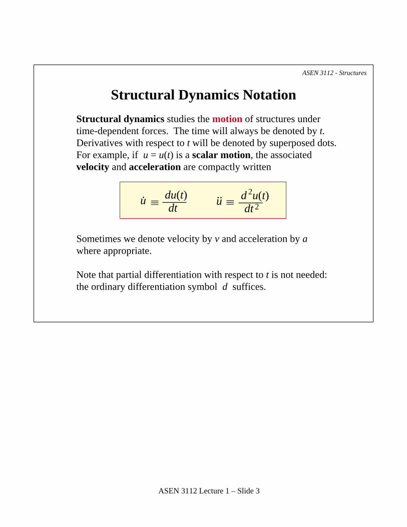
Structural dynamics studies the motion of structures undertime-dependent forces. The time will always be denoted by t.Derivatives with respect to t will be denoted by superposed dots.For example, if u = u(t) is a scalar motion, the associated velocity and acceleration are compactly written

Sometimes we denote velocity by v and acceleration by a where appropriate.

Note that partial differentiation with respect to t is not needed: the ordinary differentiation symbol d suffices.

u2

2du(t)dt

.u d u(t)

dt..


Free Undamped SDOF Oscillator: Configuration


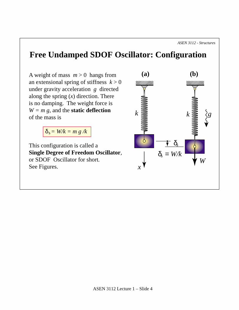
A weight of mass m > 0 hangs from an extensional spring of stiffness k > 0 under gravity acceleration g directed along the spring (x) direction. Thereis no damping. The weight force is W = m g, and the static deflection of the mass is δ = W/k = m g /k

This configuration is called a Single Degree of Freedom Oscillator, or SDOF Oscillator for short. See Figures.

��

��

sδ

sδ = W/kW

k k g

x

(a) (b)

s


Free Undamped SDOF Oscillator: Initial ConditionsASEN 3112 - Structures

��

m u..sδu=u(t)

s

s

δ = W/kW

W

k k k

(a) (b) (c)

g g

x

00

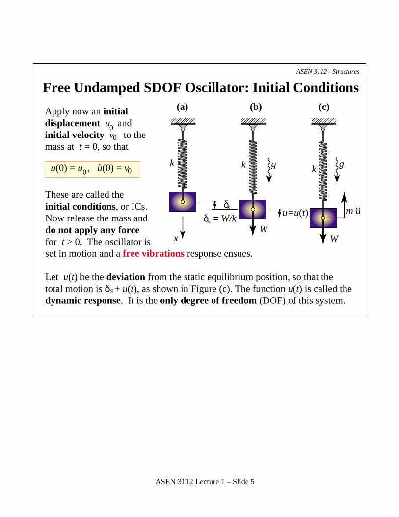
These are called the initial conditions, or ICs.Now release the mass anddo not apply any forcefor t > 0. The oscillator is set in motion and a free vibrations response ensues.

Let u(t) be the deviation from the static equilibrium position, so that the total motion is δ + u(t), as shown in Figure (c). The function u(t) is called the dynamic response. It is the only degree of freedom (DOF) of this system.

0

Apply now an initial displacement u and initial velocity v to the mass at t = 0, so that

0

u(0) = u , u(0) = v .


Free Undamped SDOF Oscillator: EOM ASEN 3112 - Structures

m u..

F = k (δ +u)s

ss

s

s

W

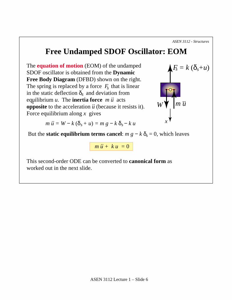
The equation of motion (EOM) of the undampedSDOF oscillator is obtained from the Dynamic Free Body Diagram (DFBD) shown on the right. The spring is replaced by a force F that is linear in the static deflection δ and deviation from equilibrium u. The inertia force m u acts opposite to the acceleration u (because it resists it). Force equilibrium along x gives

But the static equilibrium terms cancel: m g − k δ = 0, which leaves

This second-order ODE can be converted to canonical form asworked out in the next slide.

s

s

sm u = W − k (δ + u) = m g − k δ − k u..

....

x

m u + k u = 0..


Free Undamped SDOF Oscillator: Canonical EOM


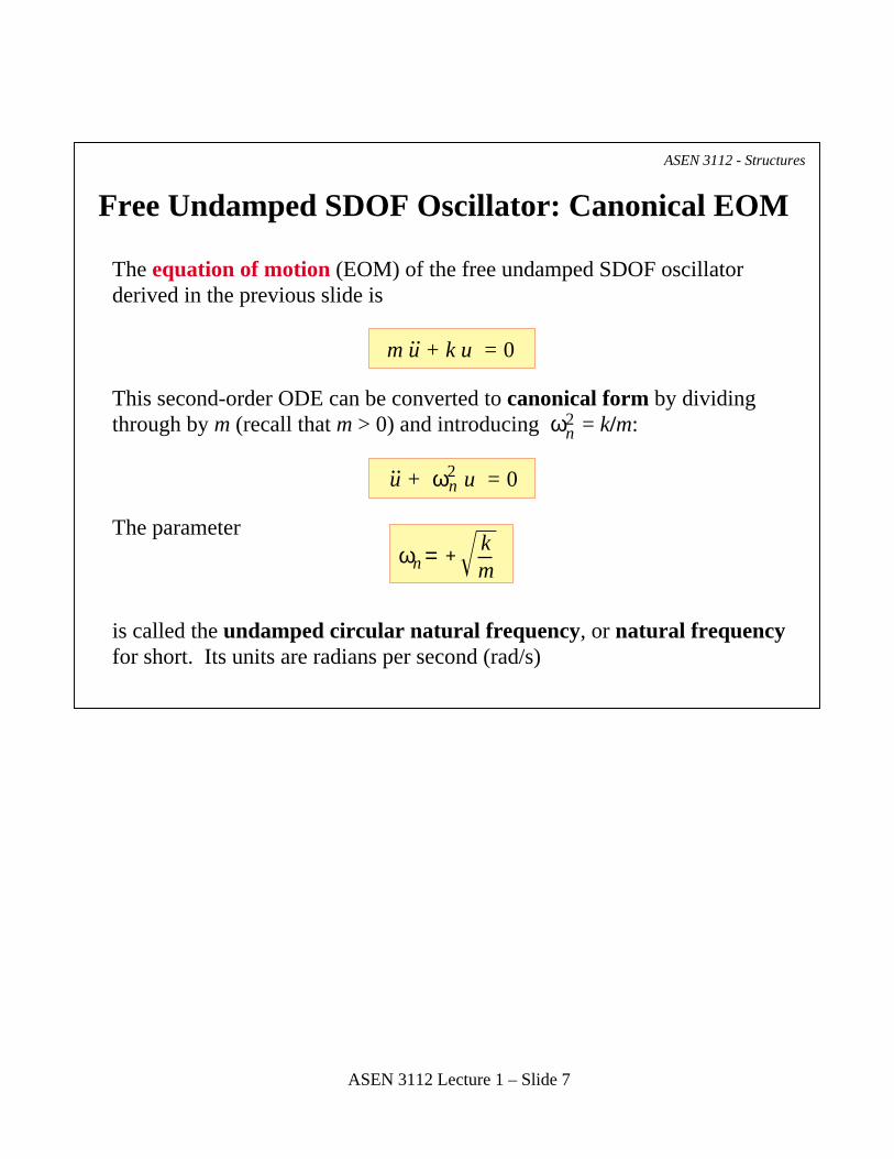
The equation of motion (EOM) of the free undamped SDOF oscillator derived in the previous slide is

This second-order ODE can be converted to canonical form by dividingthrough by m (recall that m > 0) and introducing ω = k/m:

The parameter

is called the undamped circular natural frequency, or natural frequency for short. Its units are radians per second (rad/s)

u + ω u = 0..

n

n

n2

2

m u + k u = 0..

ω = +km


Free Undamped SDOF Oscillator: EOM Features


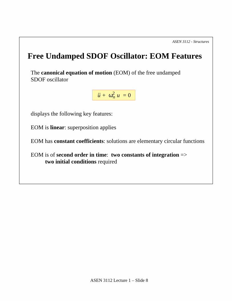
The canonical equation of motion (EOM) of the free undampedSDOF oscillator

displays the following key features:

EOM is linear: superposition applies

EOM has constant coefficients: solutions are elementary circular functions

EOM is of second order in time: two constants of integration => two initial conditions required

u + ω u = 0..

n2


Free Undamped SDOF Oscillator: Solution in Terms of Complex Exponentials


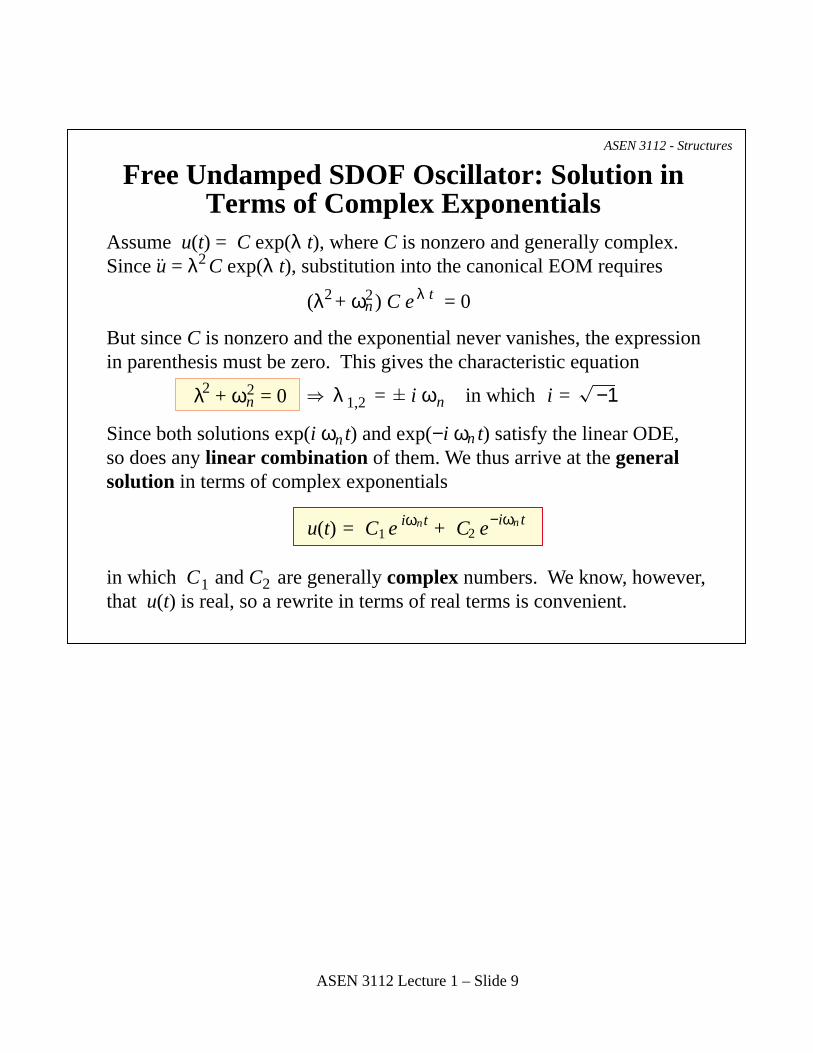
Assume u(t) = C exp(λ t), where C is nonzero and generally complex.Since u = λ C exp(λ t), substitution into the canonical EOM requires

But since C is nonzero and the exponential never vanishes, the expressionin parenthesis must be zero. This gives the characteristic equation

Since both solutions exp(i ω t) and exp(−i ω t) satisfy the linear ODE, so does any linear combination of them. We thus arrive at the general solution in terms of complex exponentials

in which C and C are generally complex numbers. We know, however, that u(t) is real, so a rewrite in terms of real terms is convenient.

2

2

2n

n

n n

1 2

(λ + ω ) C e = 0

22nλ + ω = 0

..

λ = i ω in which 1,2 i = −1

1 2u(t) = C e + C e niω t n−iω t

λ t


Free Undamped SDOF Oscillator: Solution in Terms of Trigonometric Functions


±±i θ

u(t)

u(t)

u(t)

= (C1

1 11

+ C2

2 22

) cos ωnt + i(C1 − C2) sin ωnt

= A1

1

1

cos ωnt + A2

22

sin ωn

n

t

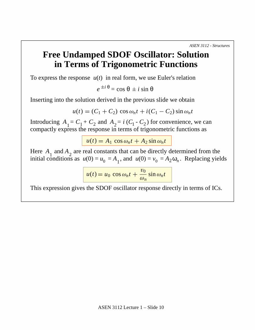
= u0 cos ωnt + v0

0 0

ωnsin ωnt

To express the response u(t) in real form, we use Euler's relation

Inserting into the solution derived in the previous slide we obtain

Introducing A = C + C and A = i (C - C ) for convenience, we can compactly express the response in terms of trigonometric functions as

Here A and A are real constants that can be directly determined from theinitial conditions as u(0) = u = A , and u(0) = v = A ω . Replacing yields

This expression gives the SDOF oscillator response directly in terms of ICs.

e = cos θ i sin θ


Free Undamped SDOF Oscillator: Phased ResponseASEN 3112 - Structures

= U cos(ωnt − α)

U =√

u20 +

(v0

ωn

)2

tan α = v0

ωn u0

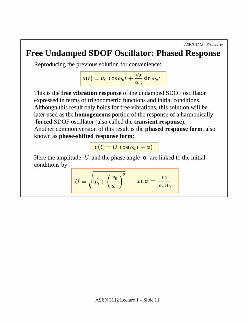
Reproducing the previous solution for convenience:

This is the free vibration response of the undamped SDOF oscillator expressed in terms of trigonometric functions and initial conditions.Although this result only holds for free vibrations, this solution will belater used as the homogeneous portion of the response of a harmonically forced SDOF oscillator (also called the transient response). Another common version of this result is the phased response form, alsoknown as phase-shifted response form:

Here the amplitude U and the phase angle α are linked to the initialconditions by

u(t)

u(t)

= u0 cos ωnt + v0

ωnsin ωnt


Free Undamped SDOF Oscillator: Effect of ICsASEN 3112 - Structures

u(t) = u0

0

0

0

cos ωnt

0

0

0

0 0

fn

n

nn

n

n

n

= ωn

2πTn = 1

fn= 2π

ωn

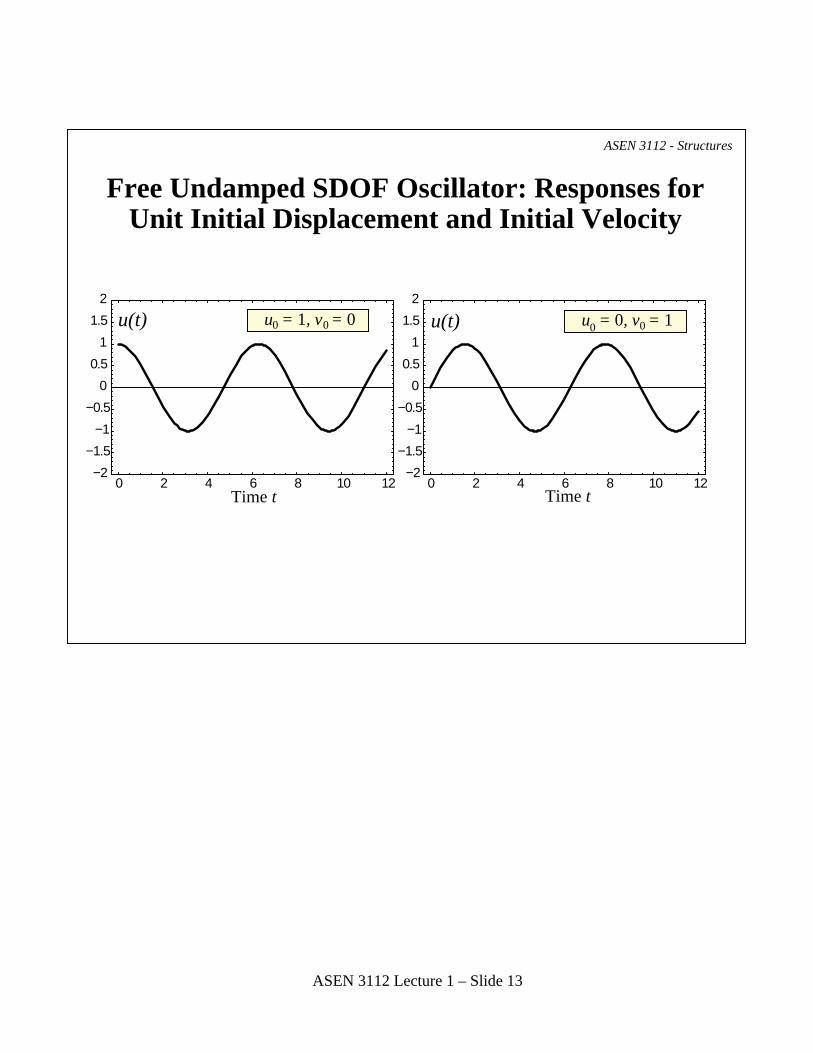
To study the effect of initial conditions, consider first the case where the massis displaced from its static equilibrium position by u and released. Then v = 0, so the response is

This is called a simple harmonic motion with amplitude u , undampednatural frequency f and undamped natural period T given by

The frequency f is expressed in cycles per second or Hertz (abbr. Hz;1 Hz = cycle/s). The period is given in seconds per cycle, or simply seconds (s).It is easily verified that for this case the phased response has U = u and α = 0.If u = 0 but v is nonzero the response is u(t) = v sin ω t/ω .This has the same frequency but amplitude v /ω and starts at zero.Plots for a unit initial displacement and initial velocity are shown on next slide.


Free Undamped SDOF Oscillator: Responses for Unit Initial Displacement and Initial Velocity


0 2 4 6 8 10 12

−1.5−1

−0.50

0.51

1.52

0 2 4 6 8 10 12

−1.5−1

−2−2

−0.50

0.51

1.52

Time t Time t

u(t) u(t)u = 1, v = 00 00 u = 0, v = 10


Free Damped SDOF Oscillator: ConfigurationASEN 3112 - Structures

��

sδu=u(t)

sδ = W/kW

k c ck

(a) (b)

g

x

The undamped SDOF oscillator is generalized by adding a viscous damperthat exerts a resisting force c uproportional to the velocity u ofthe moving mass. Here c is called the damping coefficient.Note that the static deflection of the mass does not change: δ = W/k = m g /k

This configuration is called a Damped Single Degree of Freedom Oscillator, or Damped SDOF Oscillator for short. (Viscous damping will be assumed unless the contrary is stated.) See Figures.

..

s


Free Damped SDOF Oscillator: ICsASEN 3112 - Structures

��

sδu=u(t)

sδ = W/kW

W

k c c ck k

(a) (b) (c)

g g

x

m u..

s

0

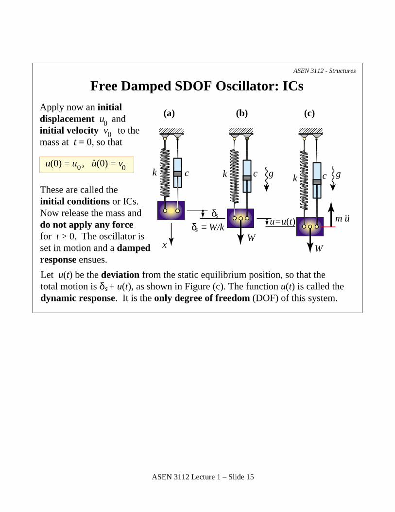
These are called the initial conditions or ICs.Now release the mass anddo not apply any forcefor t > 0. The oscillator is set in motion and a dampedresponse ensues. Let u(t) be the deviation from the static equilibrium position, so that the total motion is δ + u(t), as shown in Figure (c). The function u(t) is called the dynamic response. It is the only degree of freedom (DOF) of this system.

Apply now an initial displacement u and initial velocity v to the mass at t = 0, so that

0

0

0u(0) = u , u(0) = v .


Free, Damped SDOF Oscillator: EOM From DFBDASEN 3112 - Structures

m u..

F = k (δ +u)s s.

F = cud

W

s

d

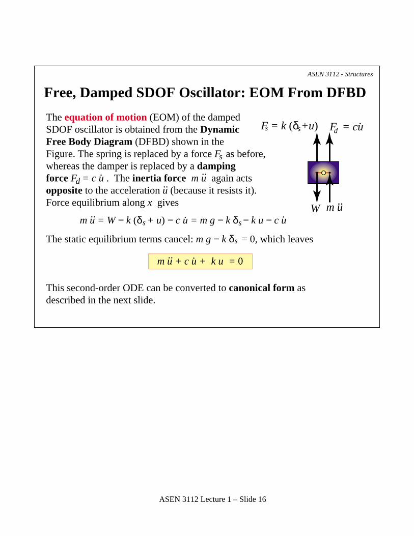
The equation of motion (EOM) of the damped SDOF oscillator is obtained from the Dynamic Free Body Diagram (DFBD) shown in the Figure. The spring is replaced by a force F as before,whereas the damper is replaced by a dampingforce F = c u . The inertia force m u again acts opposite to the acceleration u (because it resists it). Force equilibrium along x gives

The static equilibrium terms cancel: m g − k δ = 0, which leaves

This second-order ODE can be converted to canonical form asdescribed in the next slide.

s

s

sm u = W − k (δ + u) − c u = m g − k δ − k u − c u..

....

m u + c u + k u = 0..

.

.

.

.


Free, Damped SDOF Oscillator: EOM ASEN 3112 - Structures

m u + c u + k u = 0

ω2n

n

= k

m mmωn = + k

mc = 2ξωn ξ = c

2ωn

u + 2ξω

n

n u + ω2n u = 0

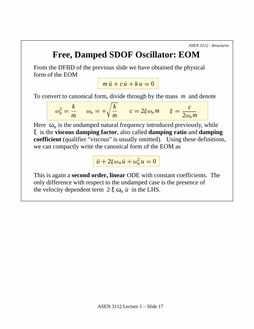
From the DFBD of the previous slide we have obtained the physical form of the EOM

To convert to canonical form, divide through by the mass m and denote

Here ω is the undamped natural frequency introduced previously, whileξ is the viscous damping factor, also called damping ratio and dampingcoefficient (qualifier "viscous" is usually omitted). Using these definitions, we can compactly write the canonical form of the EOM as

This is again a second order, linear ODE with constant coefficients. Theonly difference with respect to the undamped case is the presence of the velocity dependent term 2 ξ ω u in the LHS..


Free, Damped SDOF Oscillator: Char Equation ASEN 3112 - Structures

λ t

λ2 + 2ξωnλ + ω2n = 0

λ1,2 = −ξωn ωn ξ 2 − 1

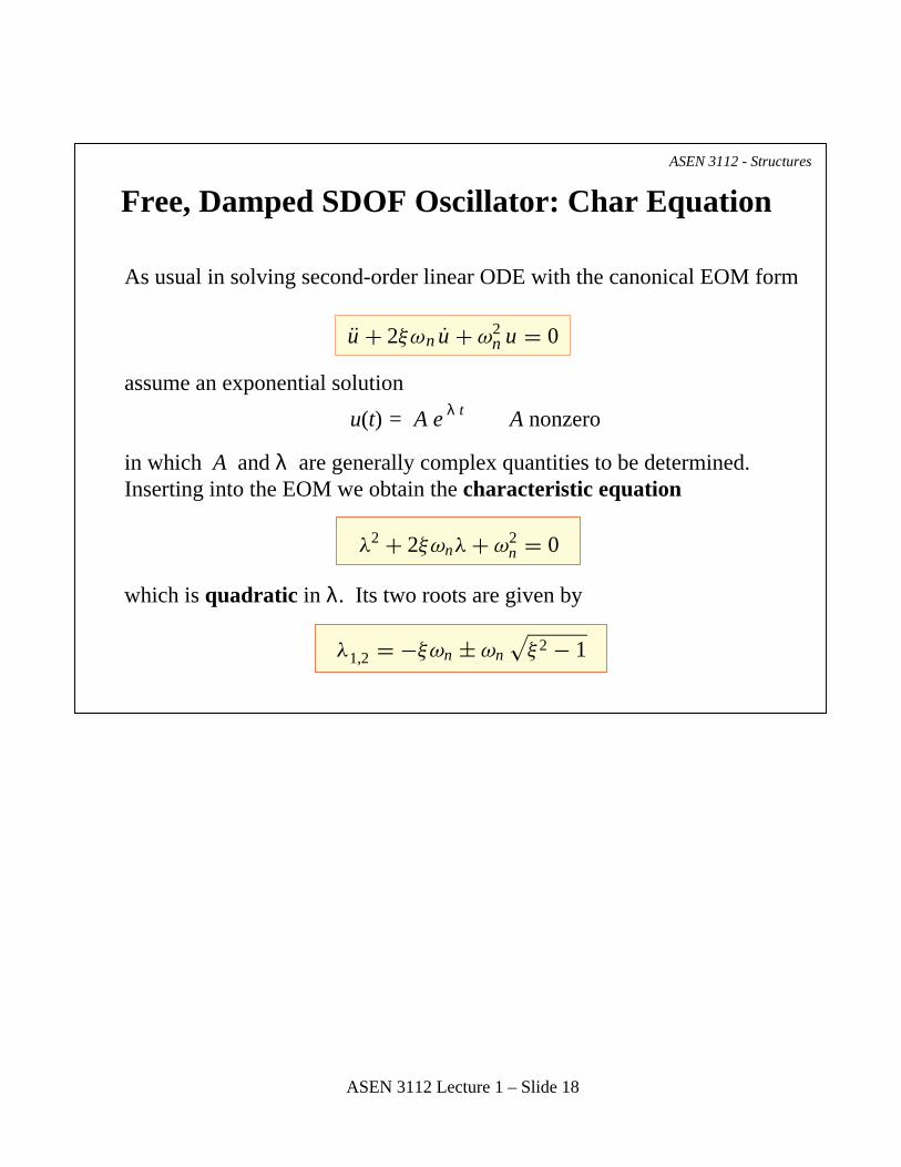
As usual in solving second-order linear ODE with the canonical EOM form

assume an exponential solution

in which A and λ are generally complex quantities to be determined.Inserting into the EOM we obtain the characteristic equation

which is quadratic in λ. Its two roots are given by

u(t) = A e A nonzero

u + 2ξωn u + ω2n u = 0


Free Damped SDOF Oscillator: Three Response Types


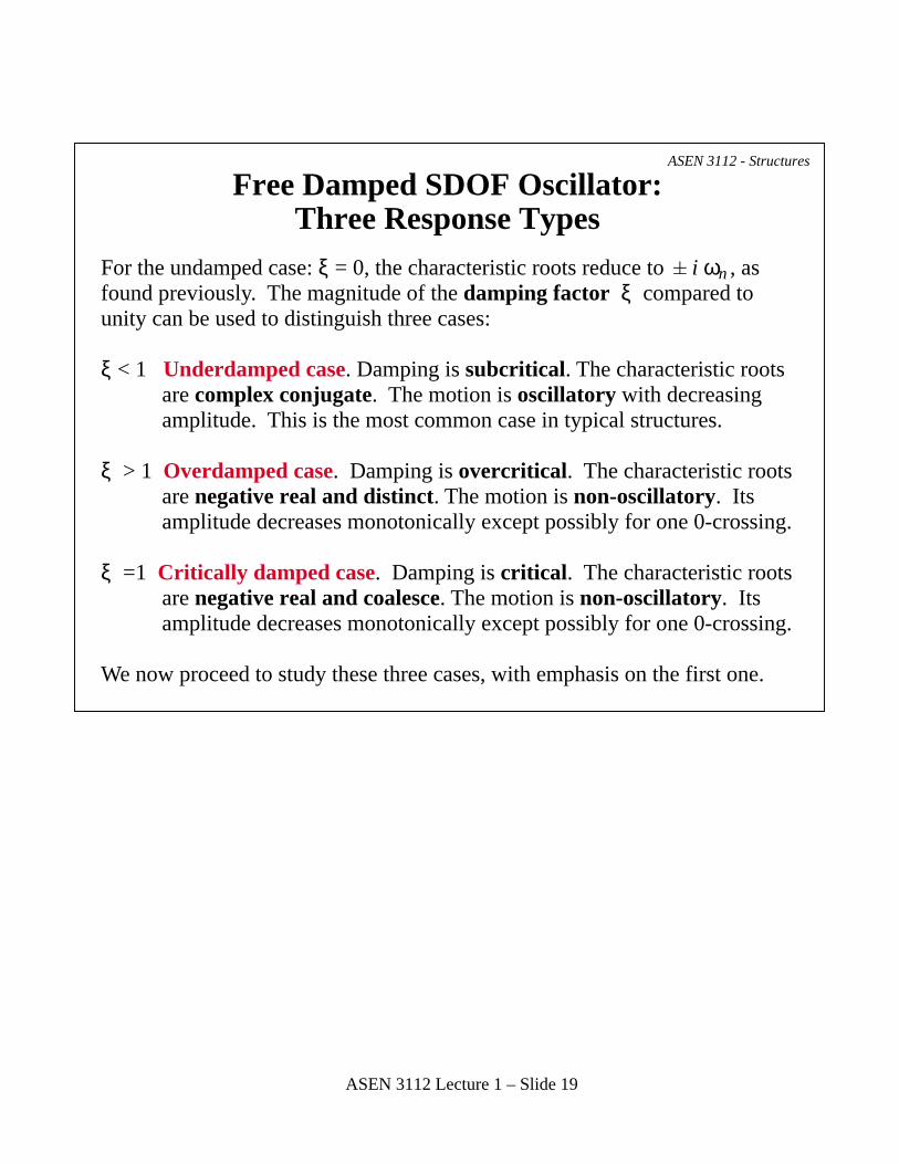
For the undamped case: ξ = 0, the characteristic roots reduce to i ω , asfound previously. The magnitude of the damping factor ξ compared to unity can be used to distinguish three cases:

ξ < 1 Underdamped case. Damping is subcritical. The characteristic roots are complex conjugate. The motion is oscillatory with decreasing amplitude. This is the most common case in typical structures.

ξ > 1 Overdamped case. Damping is overcritical. The characteristic roots are negative real and distinct. The motion is non-oscillatory. Its amplitude decreases monotonically except possibly for one 0-crossing.

ξ =1 Critically damped case. Damping is critical. The characteristic roots are negative real and coalesce. The motion is non-oscillatory. Its amplitude decreases monotonically except possibly for one 0-crossing.

We now proceed to study these three cases, with emphasis on the first one.

n


Free Damped SDOF Oscillator: Underdamped Case


λ1,2 = −ξωn ± iωd

d

ωd = ωn

n

1 − ξ 2

Td = 2π

ωd

= e−ξ ωnt ( A1 cos ωd t + A2 sin ωd t)

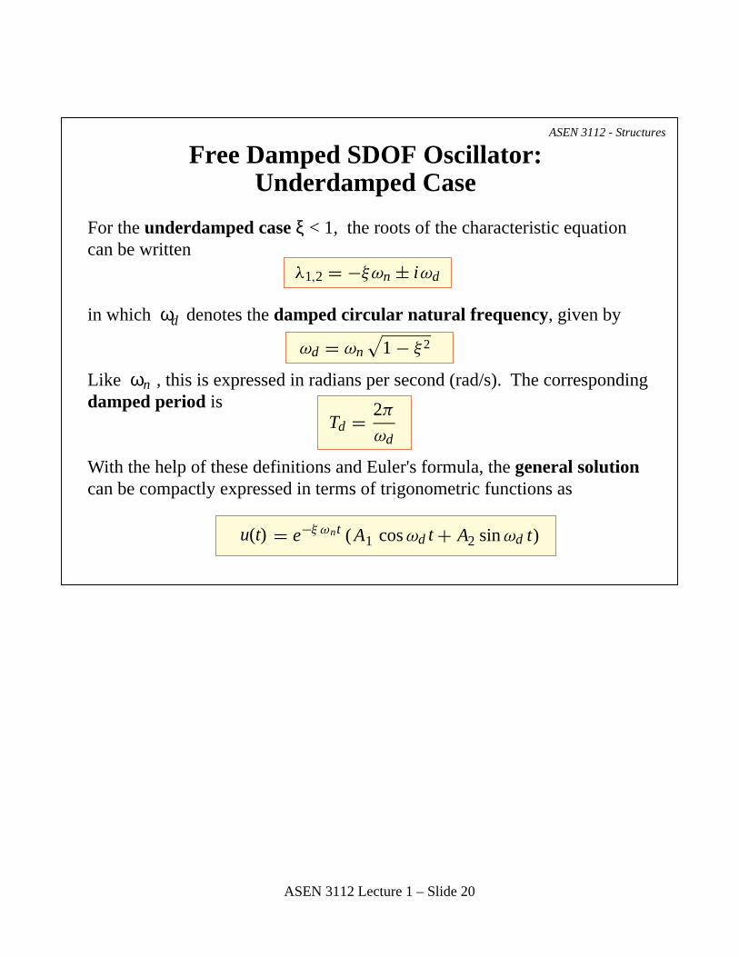
For the underdamped case ξ < 1, the roots of the characteristic equationcan be written

in which ω denotes the damped circular natural frequency, given by

Like ω , this is expressed in radians per second (rad/s). The correspondingdamped period is

With the help of these definitions and Euler's formula, the general solutioncan be compactly expressed in terms of trigonometric functions as

u(t)


Free Damped SDOF Oscillator: Underdamped Case (cnt'd)


u(t)

u(t)

= e−ξ ωn t(

u0

00

0 0

cos ωd t + v0

0

+ ξ ωn

n

u0

ωd

d

sin ωd t)

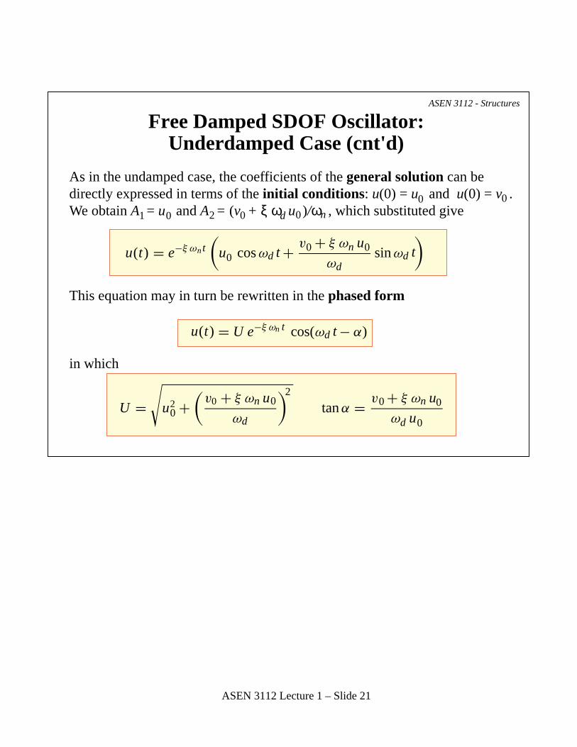
= U e−ξ ωn t cos(ωd t − α)

U = u20 +

(v0 + ξ ωn u0

ωd

)2

tan α = v0 + ξ ωn u0

ωd u0

As in the undamped case, the coefficients of the general solution can be directly expressed in terms of the initial conditions: u(0) = u and u(0) = v . We obtain A = u and A = (v + ξ ω u )/ω , which substituted give

This equation may in turn be rewritten in the phased form

in which

1 2


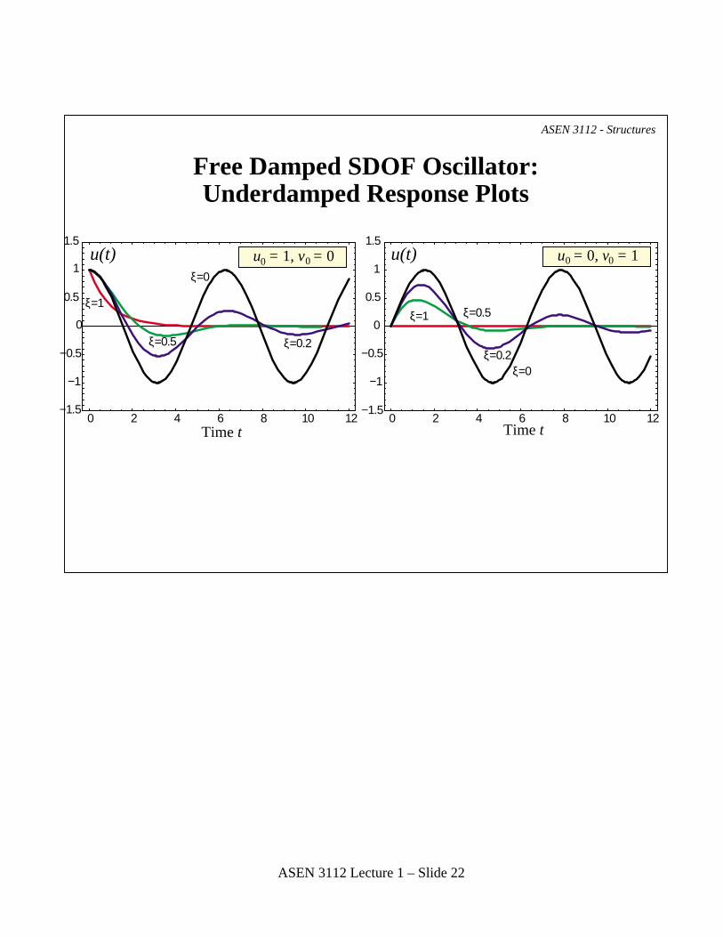
Free Damped SDOF Oscillator: Underdamped Response Plots


0 2 4 6 8 10 12

−1

−0.5

0

0.5

1

1.5

0 2 4 6 8 10 12

−1

−0.5

0

0.5

1

1.5

−1.5−1.5

Time t Time t

u(t) u(t)u = 1, v = 00 u = 0, v = 10 00

ξ=0

ξ=0.2ξ=0.5

ξ=1

ξ=0ξ=0.2

ξ=0.5ξ=1


Free Damped SDOF Oscillator: Critically Damped Case


1

1

1

2

2

2

n

0 n

n

00

If ξ = 1 the characteristic roots coalesce: λ = λ = −ω . The theory ofsecond-order linear ODE says that the solution is

in which coefficients A and A depend on initial conditions. Introducing these we arrive at the final expression for the response

Typical pictures of the response are shown on the last slide together with the overdamped case. The critically damped case responsecurves are plotted in red.

u(t) = (A + A t ) e−ω t

nu(t) = [u + (v + ω u ) t ] e−ω t


Free Damped SDOF Oscillator: Overdamped Case


u(t) = e−ξ ωn t u0 cosh ω∗t + v0 + ξ ωn u0

ω∗ sinh ω∗t

If ξ > 1 the characteristic equation has two distinct negative real roots.For convenience introduce the pseudo frequency

Then the solution may be compactly expressed in terms of the hyperbolicsine and cosine as

in which coefficients A and A depend on initial conditions. Introducing these we arrive at the final expression for the response

The effect of the damping factor ξ on the response of an overdampedSDOF oscillator may be observed in the pictures of the next slide.

1 2

ω∗ = ωn ξ 2 − 1

u (t) = e−ξ ωn t ( A1 cosh ω∗t + A2 sinh ω∗t )


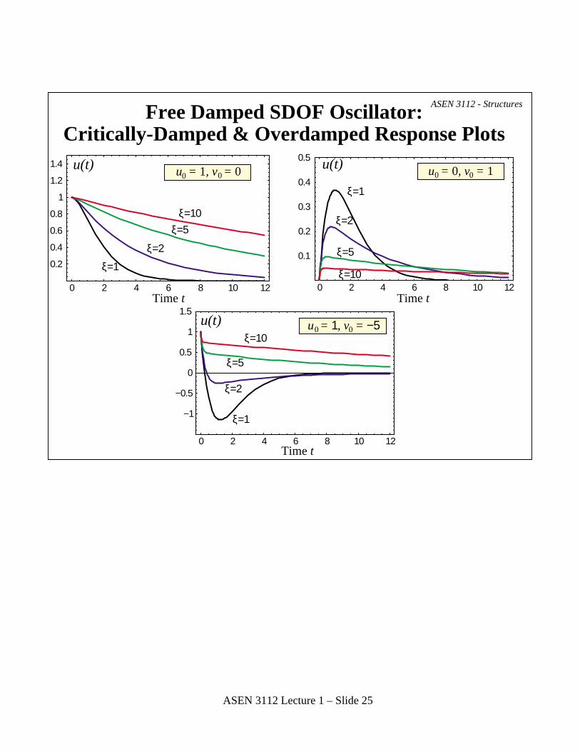
Free Damped SDOF Oscillator: Critically-Damped & Overdamped Response Plots


0 2 4 6 8 10 12

0.2

0.4

0.6

0.8

1

1.2

1.4

0 2 4 6 8 10 12

−1

−0.5

0

0.5

1

1.5

0 2 4 6 8 10 12

0.1

0.2

0.3

0.4

0.5

Time t Time t

Time t

u(t)

u(t)

u(t)

ξ=10

ξ=10

ξ=10

ξ=5

ξ=5

ξ=5

ξ=2

ξ=2

ξ=2

ξ=1

ξ=1

ξ=1

u = 1, v = 00 u = 0, v = 10 0

u = 1, v = −500

0


Documents

Free Single-DOF Oscillator - colorado.edu · ASEN 3112 Lecture 1 – Slide 1. ASEN 3112 - Structures We can go pretty fast in this ... Structural dynamics studies the motion of structures