Free Trade Agreements, Trade Openness and Economic Growth

Free Trade Agreements, Trade Openness and

Economic Growth: A study of Asia

Saian Sadat*

August 2017

Supervisor: Dr. Jean-Marie Viaene

Co-reader: Dr. Julian Emami Namini

MSc program: International Economics

Erasmus School of Economics, Erasmus University Rotterdam.

* Student number: 426763. Email: [email protected]

mailto:[email protected]

Abstract

The accelerated proliferation of the volume of FTAs for Asian economies has constantly intrigued

the economics researchers. An anonymous conclusion is yet to be reached about the effect of FTAs

on economic growth. This research investigates the affiliation amidst in-effect FTAs and trade

openness on growth. A dynamic panel approach with the Arellano-Bond GMM estimators has

been used for this research to tackle the endogeneity issue faced by past literatures. This research

enhances the current literature by scrutinizing both bilateral and multilateral FTAs in individual

models with a dummy variable approach. The inspection of the effect of FTAs on economic

development of Asian LDCs in a separate model is also a contribution of this paper to existing

literature. Individually, the FTAs failed to indicate statistically significant and positive impact on

growth. However, when tested in the presence of trade openness they do exhibit positive statistical

significance on growth. Intriguingly, trade openness exhibits a negative ramification on growth in

all estimations. The FTA dummy for the Asian LDCs demonstrates a negative outcome on

economical progression which can be attributed to the net importer characteristics of those

countries.

1

Table of Contents

1. Introduction ................................................................................................................................. 7

2. Literature Review...................................................................................................................... 10

2.1 Trade Theories and Growth................................................................................................. 10

2.2 FTA, Trade and Growth ...................................................................................................... 12

2.3 Trade Openness and Growth ............................................................................................... 14

2.4 FTA scenario of Asia ….………………………………………………………………….16

2.5 Asia and Trade Openness……….…………………...…………………………………….18

3. Methodology ............................................................................................................................ 20

3.1 Estimation Model ................................................................................................................ 20

3.2 Variables.............................................................................................................................. 21

3.2.1 Dependent Variables ..................................................................................................... 23

3.2.2 Independent Variables ................................................................................................... 23

3.2.3 Instrumental Variables .................................................................................................. 25

3.2.4 Selection of Variables…………………………………………………………….…...26

3.3 Data: .................................................................................................................................... 27

3.3.1 Data Timeline…………………………………………………………………………27

3.3.2 Data Sources …………….…………………………………………………………...28

4. Hypotheses……………………………...……………………………………………………..28

4.1 FTAs and Asia………………………….………………………………………………….28

4.2 Openness of Asia ................................................................................................................. 31

4.3 FTA and openness ............................................................................................................... 32

4.4 Growth of Least Developed Countries ................................................................................ 33

5. Empirical Outputs ..................................................................................................................... 35

5.1 Unit root tests…………………………………………………..……………....………….35

5.2 Hypotheses Estimations…………..……………………………………………………….36

5.2.1 Hypothesis 1………………………………………………………………………....36

5.2.2 Hypothesis 2………………………………………………………………………....39

5.2.3 Hypothesis 3…………………………………………………………………………42

5.2.4 Hypothesis 4…………………………………………………………………………45

2

5.2.5 Hypothesis 5………………………………………………………………………..47

5.2.6 Hypothesis 6………………………………………………………………………..50

5.2.7 Hypothesis 7………………………………………………………………………..53

5.2.9 Hypothesis 8………………………………………………………………………..55

5.2.8 Hypothesis 9………………………………………………………………………..58

6. Policy Recommendation and Future Research Prospects …………………………………..60

7. Appendix…………………………………………………………………………………….63

8. References…………………………………………………………………………………...67

3

List of Tables

Table 3.1: Variable name, description, formula and source 22

Table 4.1: In effect FTAs as of 2015 29

Table 5.1: Unit root test of ycapit 35

Table 5.2: Unit root test of TOi,t-1 36

Table 5.3: Benchmark OLS regressions without and with control variables 37

Table 5.4: Arellano-Bond estimations of the first hypothesis 38


Table 5.6: Arellano-Bond estimations of the second hypothesis 41


Table 5.8: Arellano-Bond estimations of the third hypothesis 44


Table 5.10: Arellano-Bond estimations of the fourth hypothesis 46


Table 5.12: Arellano-Bond estimations of the fifth hypothesis 49


Table 5.14: Arellano-Bond estimations of the sixth hypothesis 52


Table 5.16: Arellano-Bond estimations of the seven hypothesis 54


4

Table 5.18: Arellano-Bond estimations of the eight hypothesis 57


Table 5.19: Arellano-Bond estimations of the nineth hypothesis 59

Table A.1: Summary statistics of the untransformed variables 65

Table A.2: Summary statistics of the transformed variables and the instrumental

variable

66

Table A.3: Summary statistics of the dummy variables 66

5

List of Figures

Figure 2.1: Total and proposed number of FTAs in Asia

17

Figure 2.2: Exports of goods and services (% of GDP) for South Asian Countries

19

Figure 4.1: Asia’s share of world merchandise trade

31

Figure A.1: Distribution of trade openness for the Asian countries

63

Figure A.2: Distribution of BFTAs for the subject countries

64

Figure A.3: Distribution of MFTAs for the subject countries

65

6

Abbreviations

ADB Asian Development Bank

ADF Augmented Dickey Fuller Test

ARIC Asia Regional Integration Center

ATE Average Treatment Effect

BFTA Bilateral Free Trade Agreement

CA Comparative Advantage

CPI Consumer Price Index

FDI Foreign Direct Investment

FTA Free Trade Agreement

GMM Generalized Methods of Moments

HO Heckscher-Ohlin

IV Instrument Variable

LDC Least Developed Country

MFTA Multilateral Free Trade Agreement

OLS Ordinary Least Squares

PC Per Capita

UNCTAD United Nation Conference on Trade and Development

7

1. Introduction

“As far as we are concerned there is no protection in Protectionism”

- Jean-Claude Juncker,

President; European Commission

6th July; Brussels, Belgium.

This statement was made after European Union entered into a Free Trade Agreement (FTA) with

Japan which is deemed to be the biggest FTA of the modern age.

The definition of a Free Trade Agreement (FTA): a treaty among numerous countries to minimize

trade barriers – import quotas and tariffs; and to introduce a zone where limitation free trade in

services and merchandises is channeled across mutual borders. It is a tool for economic integration.

During the last three decades the Asian economies have significantly liberalized their international

trade through economic integrations. Along with being a part of the World Trade Organization

(WTO) the countries are now opting to establish FTA’s within themselves. Association of

Southeast Asian Nations (ASEAN) and South Asian Association for Regional Corporation

(SAARC) were created with a view to facilitate trade for their member countries within Asia.

These organizations are growing in member numbers with passing time as countries look to be

more integrated in a higher scale to reap the benefits of trade. A membership of such organizations

is lucrative as it provides an automatic access to the multilateral FTAs signed by the organization.

The number of bilateral FTAs (one-to-one FTA) has also substantially increased as countries try

to negotiate their individual needs for favorable terms of trade.

Economic integrations and FTAs are believed to foster economic growth. Among all the benefits

of such agreements this is the one that has captured the most attention from the economic

researchers. Evidence is present for both positive and negative influence of FTA on growth.1 Past

literature on the topic have failed to conclude a confirm direction of the FTA’s effect on countries

economic growth. The lack of a concrete conclusion and the rapid increase in the number of FTAs

for the Asian countries serve as motivation for the paper. The paper address the issue with a dummy

1 Detailed discussion can be found at section 2

8

variable approach which represents the concluded and in-effect FTAs for a country. The first

research question that this paper addresses is:

“Does having an in-effect FTA let it be bilateral or multilateral leads to positive economic growth

for its member country in comparison with a country with no FTA?”

The paper also investigates the consequence of trade openness on growth. Despite large number

of work an anonymous conclusion of the effect of trade openness has not been reached yet.

According to Baldwin (2003) puts it, “Because of the ambiguity of the relationship between trade

and growth, the empirical relationship remains an open one.” Harrison and Rodriguez-Clare (2009)

reviewed past studies inspecting the affinity amongst trade-openness and growth. Studies

exhibiting a positive connection amid openness and economic progress suffer from numerous

number of limitations. Two of the biggest issues of past literature are the definition of trade-

openness used by the past authors and the issue of endogeneity between trade-openness and

economic growth. Authors in the past have utilized the Gravity equation approach to tackle the

endogeneity issue. However, the Gravity model itself suffer from time invariant observations issue.

These issues have made the past estimation models subject to criticism and serves as motivation

for this paper. Therefore, the second research question becomes:

“Can greater trade integration induce positive level of growth on subject country’s economy?”

This research scrutinizes the influence of FTAs on economic growth of Least Developed Countries

(LDC) separately. DeJong and Ripoll (2006), tests cross-country data for 1975-2000 and finds

economic growth is affected through openness. However, the magnitude is restricted by the income

level. A positive link was discovered between growth rates and tariffs for world’s poorest countries

while the association was negative for rich countries. Due to lack of bargaining power to influence

the terms of trade the LDCs can suffer from adverse effect of trade. This paper suspects a negative

impact of FTAs for LDCs. The final research question of the paper is:

“Does the FTAs (both bilateral and multilateral) exhibit a negative burden on the economic

development of LDCs?”

Past studies have used trade openness and trade volume interchangeably. This study explores the

effect of trade openness on growth with an index for trade openness. The endogeneity of the FTA

and trade openness is repeatedly stated in past literature. To manage the issue of endogeneity this

9

research uses a dynamic panel model approach. The Arellano-Bond approach for estimating

dynamic panel model uses lags of the dependent and independent variables instrument variables.

A separate instrument variable for trade openness is also used along with the lagged instrument

variables. Furthermore, the openness indicator is tested in lagged form to tackle the issue of reverse

causality. The models are tested in the presence of a set of six control variables.

The dynamic panel model is estimated for 31 Asian countries including seven out of nine LDCs

of the region. The time line is 1990-2013 as the FTAs are a relatively new notion for Asian

economies. To reveal the actual effect of FTA on growth only the in-effect FTAs are considered

in this study leaving out the FTAs those which are under negotiation or have been signed but not

called into effect yet. The different models are estimated with a strongly balanced panel dataset.

The effect of FTAs on economic growth is tested in two separate models. One model tests the

FTAs independently and the other model tests the FTAs in presence of trade openness. When

tested individually, both formation of the FTAs fail to exhibit a positive impact on economic

growth of Asian countries. Intriguingly, when tested in the presence of trade openness both dummy

variables for bilateral and multilateral FTA exhibit a positive and statistically significant effect on

economic growth. These findings is in agreement with Nunn and Trefler (2004), who have shown

countries with controlled trade openness experience higher growth.

The trade openness variable is statistically significant throughout the models as expected.

However, interestingly enough it demonstrates a negative sign in all the estimations. Although this

finding may be infrequent it is not unprecedented. Chang, Kaltani, and Loayza (2009) show that

the growth effect of trade openness is significantly positive only if certain complementary

domestic reforms are undertaken, including deregulations of business, financial developments,

better education, rule of law, labor market flexibility, etc.

The dummy variable of FTAs for LDCs appears with a negative coefficient value. Both bilateral

and multilateral FTAs exhibit negative effect on economic growth for LDCs. FTAs eliminates

import tariffs which can be crucial in protecting domestic industries from rigorous international

competition. Harrison and Rodriguez-Clare (2009) reviewed studies that show industrial policies

which offers a degree of protection tend to have a positive effect on economic growth of those

countries that lack comparative advantage in trade. This is discussed in depth later in the paper.

10

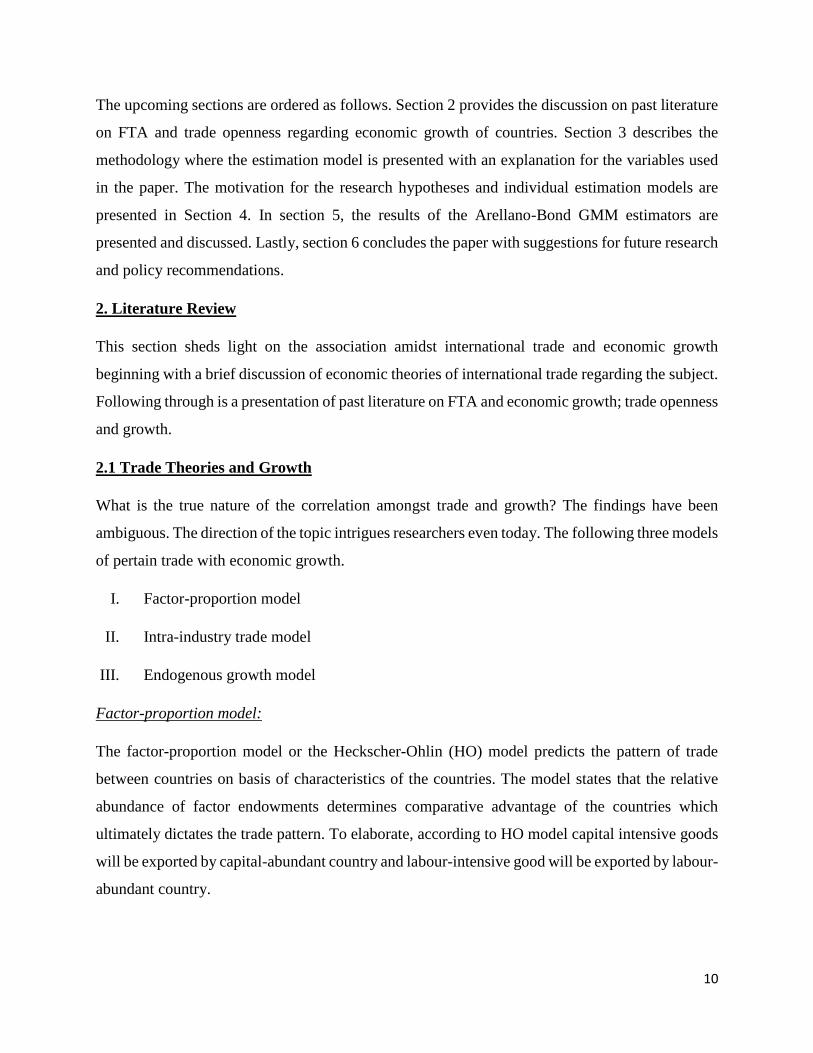
The upcoming sections are ordered as follows. Section 2 provides the discussion on past literature

on FTA and trade openness regarding economic growth of countries. Section 3 describes the

methodology where the estimation model is presented with an explanation for the variables used

in the paper. The motivation for the research hypotheses and individual estimation models are

presented in Section 4. In section 5, the results of the Arellano-Bond GMM estimators are

presented and discussed. Lastly, section 6 concludes the paper with suggestions for future research

and policy recommendations.

2. Literature Review

This section sheds light on the association amidst international trade and economic growth

beginning with a brief discussion of economic theories of international trade regarding the subject.

Following through is a presentation of past literature on FTA and economic growth; trade openness

and growth.

2.1 Trade Theories and Growth

What is the true nature of the correlation amongst trade and growth? The findings have been

ambiguous. The direction of the topic intrigues researchers even today. The following three models

of pertain trade with economic growth.

I. Factor-proportion model

II. Intra-industry trade model

III. Endogenous growth model

Factor-proportion model:

The factor-proportion model or the Heckscher-Ohlin (HO) model predicts the pattern of trade

between countries on basis of characteristics of the countries. The model states that the relative

abundance of factor endowments determines comparative advantage of the countries which

ultimately dictates the trade pattern. To elaborate, according to HO model capital intensive goods

will be exported by capital-abundant country and labour-intensive good will be exported by labour-

abundant country.

11

The HO model itself doesn’t exhibit the direct relation between trade and growth; the Rybczynski

theorem- dynamic version of HO sheds light on the subject. Under the assumption of the abundant

factor being capital it assumes that ultra-biased growth along the capital-expansion path will be

reached by the country.

Intra-industry trade model:

Substantial empirical studies of international trade have argued that conventional theories of

comparative advantage cannot effectively explain the trade among the industrial countries. Two

stylized facts of world trade can provide explanation to the contradiction of traditional theories.

First- majority of world trade is conducted among countries with analogous factor endowments.

Second- the nature of trade between identical countries is fundamentally introductory; implying

the trade consists of two-way transaction in parallel goods. The inter-industry specialization and

trade is a result of orthodox forces of CA operating on groups of products. Nevertheless, existence

of scale economies in production limits the diversity of merchandises produced by a country.

Hence identical countries will have an incentive to trade, usually in goods manufactured with

analogous factor proportions and this trade does not include distributional effect of income. These

economies of scale emerging in intra-industry trade are thought to pave the way for rapid

productivity gains and thus accelerated growth (Krugman, 1981).

Endogenous growth model:

Endogenous growth theory states economic growth is mainly the result of endogenous factors and

not exogenous forces. It states that investment in human capital, innovation, and knowledge are

substantial patrons of economic growth. It further explains the aspect of spillover effects and

positive externalities of a knowledge-based economy which leads to economic growth. The

implication of the theory is that policies increasing the openness and competitiveness of the

economy will foster growth.

Foreign direct investment (FDI) increases knowledge spillovers across countries (Barro and Sala-

i-Martin, 1995). Both physical and human capital experiences productivity increase through

spillovers. Production efficiency enrichment of endogenous growth factors can be extended with

supplementary Research and Development and with learning-by-doing. In this model, investment

12

or trade first affect the productivity of endogenous growth factors and then the economic progress

of a country.

2.2 FTA, Trade and Growth:

Having experienced the rapid rise in the volume of Free Trade Agreements among countries, both

bilateral and multi-lateral; in last two decades one can be led to assume that FTAs have positive

effect on the country’s income. However, there is little empirical support from the international

economists to the claim of a positive effect of FTAs on country’s income due to lack of reliable

quantitative estimation methods.

The vast majority of the past literature on FTAs has been concentrated on examining the effect of

FTAs on member countries trade flows rather than investigating a direct link of FTAs with the

economic growth of the member countries. “Gravity Equation” has been the most popular

approach in the past literature to study the effect of FTAs on bilateral trade flows. Noble laureate

Jan Tinbergen (1962) was the first to publish an econometric study using the gravity equation for

international trade flows. His work which included evaluation of FTA dummy variables on trade

which showed insignificant ATE of FTAs on trade flows.

Past literature of gravity equation typically applied cross-sectional data for a particular year or

multiple years pooled together and used a dummy variable representing the absence or presence

of an FTA to estimate the ATE of an FTA on member countries' bilateral trade flows (Aitken

(1973) and Baldwin (1994)). Following this particular method Aitken (1973) found positive and

statistically significant effect of European Commission on its members trade flows. However,

coefficient estimation of such dummy variable frequently depicts extreme volatility across years.

In numerous cases seemingly successful economic integrations– such as the European Union

(formerly, European Economic Community) – have negative estimated treatment effects, Frankel

(1997). This vulnerability of estimated FTA treatment effects was addressed by Ghosh and

Yamarik (2004). They applied extreme-bounds analysis to test the robustness of FTA dummy

coefficient estimates and found empirical evidence using cross-section data that estimated ATE of

most FTAs are “fragile”; pointing out the fact that there are still no consistent ex post estimates of

ATE of the FTAs.

13

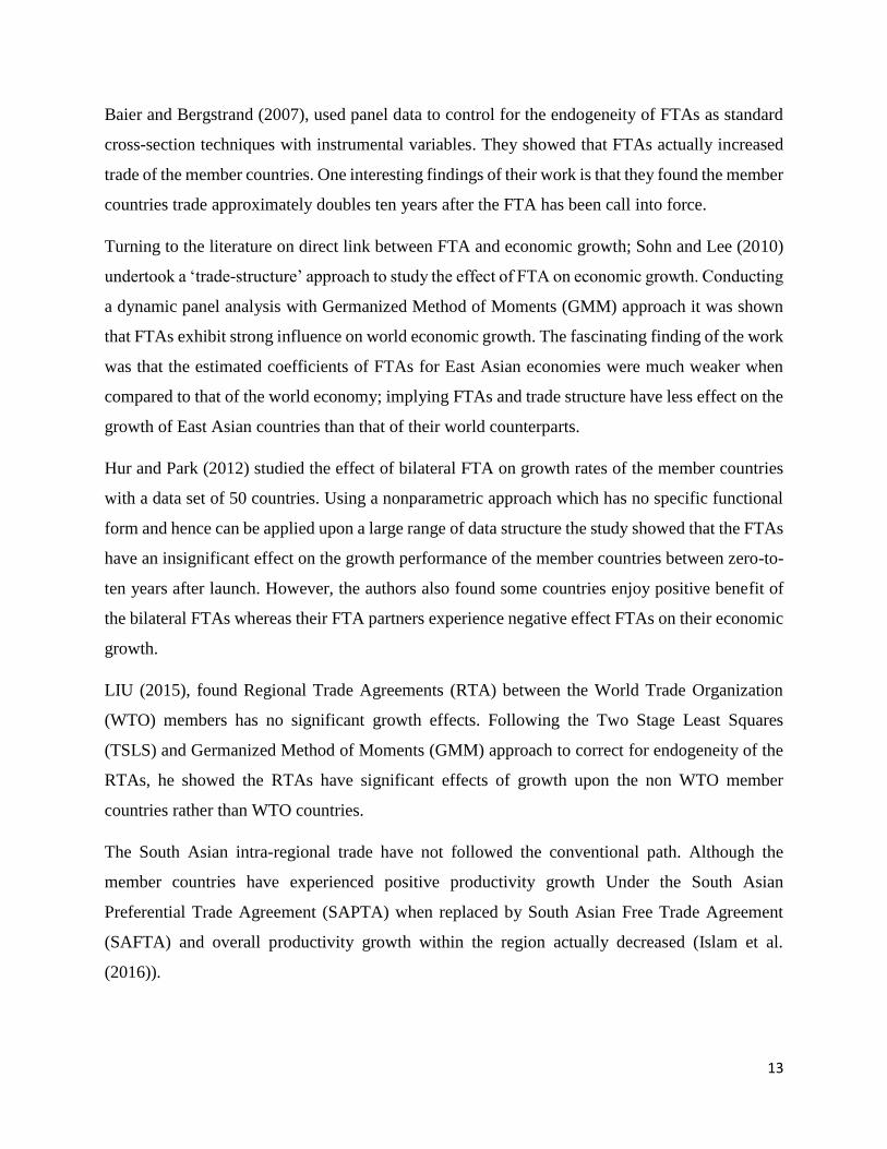
Baier and Bergstrand (2007), used panel data to control for the endogeneity of FTAs as standard

cross-section techniques with instrumental variables. They showed that FTAs actually increased

trade of the member countries. One interesting findings of their work is that they found the member

countries trade approximately doubles ten years after the FTA has been call into force.

Turning to the literature on direct link between FTA and economic growth; Sohn and Lee (2010)

undertook a ‘trade-structure’ approach to study the effect of FTA on economic growth. Conducting

a dynamic panel analysis with Germanized Method of Moments (GMM) approach it was shown

that FTAs exhibit strong influence on world economic growth. The fascinating finding of the work

was that the estimated coefficients of FTAs for East Asian economies were much weaker when

compared to that of the world economy; implying FTAs and trade structure have less effect on the

growth of East Asian countries than that of their world counterparts.

Hur and Park (2012) studied the effect of bilateral FTA on growth rates of the member countries

with a data set of 50 countries. Using a nonparametric approach which has no specific functional

form and hence can be applied upon a large range of data structure the study showed that the FTAs

have an insignificant effect on the growth performance of the member countries between zero-to-

ten years after launch. However, the authors also found some countries enjoy positive benefit of

the bilateral FTAs whereas their FTA partners experience negative effect FTAs on their economic

growth.

LIU (2015), found Regional Trade Agreements (RTA) between the World Trade Organization

(WTO) members has no significant growth effects. Following the Two Stage Least Squares

(TSLS) and Germanized Method of Moments (GMM) approach to correct for endogeneity of the

RTAs, he showed the RTAs have significant effects of growth upon the non WTO member

countries rather than WTO countries.

The South Asian intra-regional trade have not followed the conventional path. Although the

member countries have experienced positive productivity growth Under the South Asian

Preferential Trade Agreement (SAPTA) when replaced by South Asian Free Trade Agreement

(SAFTA) and overall productivity growth within the region actually decreased (Islam et al.

(2016)).

14

To sum it up, researchers are yet to be find a concrete answer to the question whether FTAs have

positive effect on countries economic growth or not, which serves as inspiration for this paper.

2.3 Trade Openness and Growth:

According to Busse and Koeniger (2012), trade is believed to foster the efficiency of resource

allocation, allowing a country to realize economies of scale and scope, support technological

progress, inspire the transmission of knowledge, and increase competitiveness in both domestic

and international markets, leading to an escalation of production line and moreover to the

development of new products. While recent empirical literature and research support this view,

little more than a decade ago the discussion of the topic seemed undecided as there was evidence

for both results: trade openness and trade barriers promoting growth.

The first era of globalization has experienced a tariff-growth paradox. Average tariff rates, which

are ought to hinder trade, had significant-positive relationship with total factor productivity growth

for 1980-1990 (Rodriguez and Rodrik, 2001). Positive association between import tariffs and

economic growth were also reported by Rodrik (2001) with graphical evidence for 1990s. In the

same light, Yanikkaya (2003) examines the relationship between growth and trade restrictions and

finds contradictory outcomes to the orthodox view on the issue, confirming that trade barriers in

form of tariffs can actually be advantageous for developing countries’ economic growth under

certain conditions.

Rruka (2004) provides additional evidence supporting Yanikkaya’s findings that appropriate

tariffs indeed appear to provide for higher levels of economic growth through adequate protection

from international trade. However, the sector on which the protection is applied is shown to be a

crucial factor. Nunn and Trefler (2004) found growth is rapid for countries that protect skill-

intensive sectors when compared to countries which protect unskilled-labor-intensive industries.

Lehmann and O’Rourke (2008) found what you protect matters. They found evidence that policies

are much likely to have the desired outcome if the pattern of protection is skewed towards sectors

yielding increasing returns that provides important externalities compared to protection is given to

declining sectors or sectors with-out externalities. This finding is also supported by Grossman and

Helpman (1991).

15

Abbas (2014) examined impact of trade liberalization on economic growth and showed increased

trade liberalization deteriorates economic growth of both developing and least developed

countries.

On the other side, International bodies argue generally for a positive relationship between trade

openness and growth. The OECD (1998, 36) states: “More open and outward-oriented economies

consistently outperform countries with restrictive trade and [foreign] investment regimes.”

According to the International Monetary Fund (IMF; 1997, 84): “Policies toward foreign trade are

among the more important factors promoting economic growth and convergence in developing

countries.” Sachs and Warner (1995), using an openness index rather than trade barriers, give

supporting evidence to the claim that outward-oriented economies consistently outperform inward-

oriented economies, with the conclusion that openness leads to more economic growth.

The conventional approaches, which were mainly used before the millennial, oversee the fact that

the openness indicators are in many cases likely to be endogenous and hence, lead to biased results

(Rodriguez and Rodrik, 1999). Rodriguez and Rodrik argue that the explanatory power of trade

barriers are often correlated with other growth-inhibiting factors such as governance; or at best

represents a proxy for general economic performance. Frankel and Romer (1999) which was

published by in the same year as Rodriguez and Rodriks’ critique; introduced an instrumental

variable approach to the trade-openness-and-growth-topic, using a Gravity model for the IV-

regression. Comparing their results of the standard OLS estimates with those of the IV-regression,

they argue that there is no evidence that OLS estimates overstate the effects of trade on income

growth. Their findings suggest that trade has a quantitatively large and robust positive effect on

income and that OLS merely underestimates the effect of the trade share on income.

While testing influence of trade openness on income through trade volume and tariff measures no

systematic effect was found on the income share of the poorest countries (Dollar and Kraay, 2004).

Interestingly, when they tested the impact of trade openness through decade-to-decade change in

trade volume with an instrumental variable approach the results turned in favour of trade. Using

lagged trade volume as instrument for current trade volume over cross-sectional data, the findings

indicated that changes in growth rates of the economies are highly correlated with the changes in

the trade volume.

16

A Frankel-Romer instrument was imitated by Ferrarini (2010) from a global trade matrix for 1990–

2007 period of 157 countries. It was deployed to evaluate the direction of the relationship between

trade and income. Results from the panel instrumental variable regression confirms rise of income

on average across trading nations triggered by international trade, particularly this effect appears

to be strongest for countries of developing Asia. Distinctively, country-size which was thought to

be a representation of domestic trade potential was found to be less an appropriate feature in

clarifying the increase of income in developing Asia.

Despite evidence of positive effect of trade openness on economic growth, the presence of negative

effect of trade openness in past literature is also not negligible. The shortage of guaranteed

direction of the impact of trade openness serves as motivation to investigate this issue in this

research.

2.4 FTA Scenario of Asia

The notion of Free Trade Agreements were slow for Asian economies during the end period of the

twentieth century. A meager number of three FTAs were in force in East Asia, including the

ASEAN Free Trade Area (AFTA) in 2000. Fascinatingly, the quantity of FTAs in the region

augmented more than tenfold in just a decade. Rapid growth in the FTA initiatives in Asia are

attributed to the following four main factors by Kawai and Wignaraja (2011/2014):

(i) Deepening market-driven economic integration in Asia,

(ii) European and North American economic integration,

(iii) The 1997–1998 Asian financial crisis, and

(iv) Slow progress in the WTO Doha negotiations

First, the market-driven economic integration through trade, FDI, and the formation of production

networks between East Asian economies. The world economy is increasingly becoming

interconnected and to sustain in a competitive world, trade integration between the countries are

crucial. The policymakers of Asia believe that FTAs can be used as a tool to eliminate the cross-

border obstacles and promote the growth of trade and FDI. Hence, FTAs are regarded a policy

framework to expand the production networks formed among the global Multi-National

Companies (MNC) and the East Asian firms.

17

Second, North American and European developed countries forming regional economic

agreements i.e. North American Free Trade Agreement (NAFTA) and European Union have

inspired East Asian FTAs. The expansion of EU to the Baltic region and the success of NAFTA

made the Asian economies realized the necessity to create economic integration to strengthen their

negotiation authority, improve international competitiveness and raise their voice on global trade

issues.

Third, financial crisis of 1997–1998 in Asia served as a wake-up call for the Asian economies.

During the Crisis Thailand suffered the most. The debt-to-GDP ratio shot up beyond 180% in the

four major ASEAN countries. The crisis made the Asian countries realize that in order to sustain

growth and stability they need to work together in the area of trade and investment by addressing

mutual obstacles. Owing to time consuming nature of the targets, they are not yet fulfilled by either

regional cooperation or national policies. Nevertheless, following the rise of FTAs in the region

especially with the largest economies of the regions- Japan and China, a number of other countries

have begun to bandwagon of these initiatives out of fear of rejection.

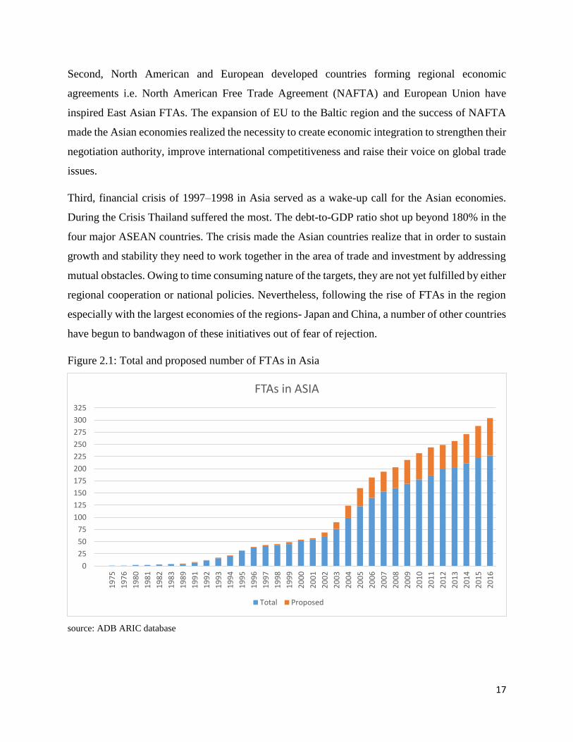
Figure 2.1: Total and proposed number of FTAs in Asia

source: ADB ARIC database

0

25

50

75

100

125

150

175

200

225

250

275

300

325

19

75

19

76

19

80

19

81

19

82

19

83

19

89

19

91

19

92

19

93

19

94

19

95

19

96

19

97

19

98

19

99

20

00

20

01

20

02

20

03

20

04

20

05

20

06

20

07

20

08

20

09

20

10

20

11

20

12

20

13

20

14

20

15

20

16

FTAs in ASIA

Total Proposed

18

Fourth, the slow progress of the WTO Doha Development Round negotiations. Beginning in

November 2001 the WTO Doha Development Round aimed to promote trade-led growth in least

developed countries. The major focused points were liberalization of two key areas: market access

for agricultural and non-agricultural goods. Unfortunately thirteen years after the initiation of the

Doha Development Round it failed to successfully conclude the negotiations which led the Asian

countries seek the FTAs as an alternative approach and resulted in a surge in the number of FTAs.

This phenomenon is fairly evident from the graph above which demonstrates the surge in FTA

numbers for the Asian region. The number of FTA in 1975 and in 1989 was only one and four

respectively. From that not only the number of signed FTAs has increased significantly to 232

FTAs in 2017; but also higher number of FTAs are being proposed, 90 in 2017 by the Asian

countries both in form of bilateral and multilateral partnerships.

2.5 Asia and Trade Openness

The emergence of Asia in the world economy as factory economy over the fifty year period from

the back-dated agricultural economy is considered as an economic miracle (Stiglitz, (1996)). In

1950, East Asia (excluding China and Japan) were lagging behind Latin America which was the

most developed region outside the industrial countries, with an average level of real GDP per

capita more than 2.5 times than that of East Asian countries. During the period of 1950s and 1960s

Asia had little prospect of economic advancement as the countries were burdened with high

poverty levels and lacked natural resources to boost the economy. A long period of policies

directed towards creating market driven expansion of international trade and FDI assisted Asia to

become the ‘global factory’ that the world sees today. Needless to mention, FTA and openness of

the economies both have played vital parts in creating the modern factory Asia.

Since 1980s, Asian countries emerged in the stage of global economy. In 1985, Asia accounted for

19% of total world export. The leading economies such as Japan and China shifted towards

manufacturing economies from agricultural economic systems. In 1995, Japan was the third largest

country in the world in terms of total export. China overtook Japan in 2004 to become the biggest

exporting economy in Asia and the third largest in the world. By 2009 China replaced Germany

as the world’s leading exporter. Since then China has kept the position of world largest exporter

economy strongly under its belt. Not only the East Asian economies but also the countries of South

Asia are also letting their presence known in the global stage especially in the Ready-made-

19

Garments (RMG) sector. Bangladesh - a South Asian least developed country is the second largest

exporter of RMG in the world after China. The South Asian economies are exhibiting a greater

degree of openness through their export orientated economies. The following diagram

demonstrates the percentage share of exports in country’s GDP for South Asian countries.

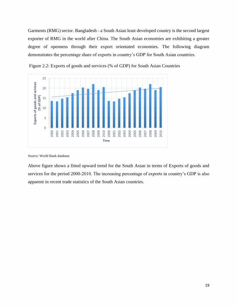
Figure 2.2: Exports of goods and services (% of GDP) for South Asian Countries

Source: World Bank database

Above figure shows a fitted upward trend for the South Asian in terms of Exports of goods and

services for the period 2000-2010. The increasing percentage of exports in country’s GDP is also

apparent in recent trade statistics of the South Asian countries.

0

5

10

15

20

25

20

00

20

01

20

02

20

03

20

04

20

05

20

06

20

07

20

08

20

09

20

10

20

00

20

01

20

02

20

03

20

04

20

05

20

06

20

07

20

08

20

09

20

10

Exp

ort

s o

f go

od

s an

d s

erv

ice

s(%

of

GD

P)

Time

20

3. Methodology

A formal model for the estimation is created in this section. A description of the variables used in

the estimation process and the sources of data are also presented in this section.

3.1 Estimation Model

Majority of past literature on FTA used the Average Treat Effect (ATE) with a probit model to

determine the effect of FTAs on cross-sectional data. Instrumental variables (IV) were introduced

to tackle the issue of endogeneity. However, despite trying a wide range of instrumental variable

the results were inconsistent. The IVs used by the past authors which are correlated cross-

sectionally with FTA are also correlated cross-sectionally with other variables. This made the

problem of endogeneity persist in cross sectional studies such as the gravity model studies on FTA.

Later it was concluded, the IV estimations of the cross-sectional data are not a reliable method for

the endogeneity issue of FTAs (Baier and Bergstrand, (2007)).

This paper uses dynamic panel model approach for this research. Random and fixed effect methods

will lead to biased estimator in this particular case. A traditional random effect approach on panel

data will lead to biased estimation of the parameters as it cannot account for the unobservable time-

invariant heterogeneity among the countries. In fixed effect model, the underlying assumption is

that the regressors are correlated to the time-invariant unobserved component. Correlation between

observables and unobservables creates endogeneity problem which produces inconsistent

estimations parameters if orthodox linear panel-data estimators are used. Possible solution would

be to take the first difference for the relationship of interest. For instance, when one wants to

estimate the following relationship:

yit = αi + γyi(t−1) + βjXit + εit (3.1)

Where y is the real per capita growth rate of GDP between period t-1 and t. i, t and j represnts

countries i Є (1,2, ……, N), time periods t Є (1990,1991,……,2013) and variables j Є (1,2, ……,

n) respectively. X is the vector containing main interest variable FTA dummies and trade openness

along with other control variables. The β captures the variable’s effect on growth. Lastly, ε is the

error term. Taking the first differences will result in the following:

Δyit = γΔyi(t−1) +βjΔXit + Δεit (3.2)

21

Unfortunately, even after the transformation to the first differences this strategy will not work as

yi(t−1) in Δyi(t−1) is a function εit-1 which is also in Δεit. Therefore, implying E(Δyi(t−1)Δεit)≠0.

This correlation can be corrected using instrumental variables. Now the question becomes which

instrumental variable? Arellano and Bond (1991), revealed the construction of estimators on the

basis of moment equations constructed from further lagged levels of yit and first-differenced errors.

Assumption of Generalized Method of Moments (GMM): particular lagged levels of the dependent

variable are orthogonal to the differenced disturbances is used to create GMM-type moment

conditions. Following this framework Arellano-Bond suggests the second lags of the dependent

variable and all the feasible lags thereafter are reliable IVs for the purpose of estimation. Thus, the

above linear dynamic model is estimated using Xi(t-2), Xi(t-3),…… and yi(t-2),yi(t-3)…. and so on as

instruments for the entire period of the data.

In order to the Arellano-Bond IVs to hold the following condition must hold:

E(Δyi(t−T)Δεit)=0 for T ≥2 (3.3)

Which implies the differenced unobserved time-invariant component should be unrelated to the

second lag of the dependent variable and the lags thereafter. This solves the problem of

endogeneity. The statement also indicates absence of serial correlation in εit. This leads to

consistent estimator under heterogeneity.

First two models are estimated for bilateral and multilateral dummy variables. In the third model

trade openness is introduced. In fourth and fifth model the FTA dummies are tested in the presence

of trade openness. The last four model examines the effect of FTAs on LDCs by introducing

separate dummy variable for both bilateral and multilateral FTAs for the LDCs. The LDC dummy

variables are also investigated together with trade openness for scrutiny. In every model for trade

openness an instrumental variable has been used to tackle endogeneity.

3.2 Variables

An overview of the dependent, independent and instrumental variable of the growth regression is

presented in this section. Discussion regarding the selection of explanatory variables compared to

standard variables is also offered in the section.

22

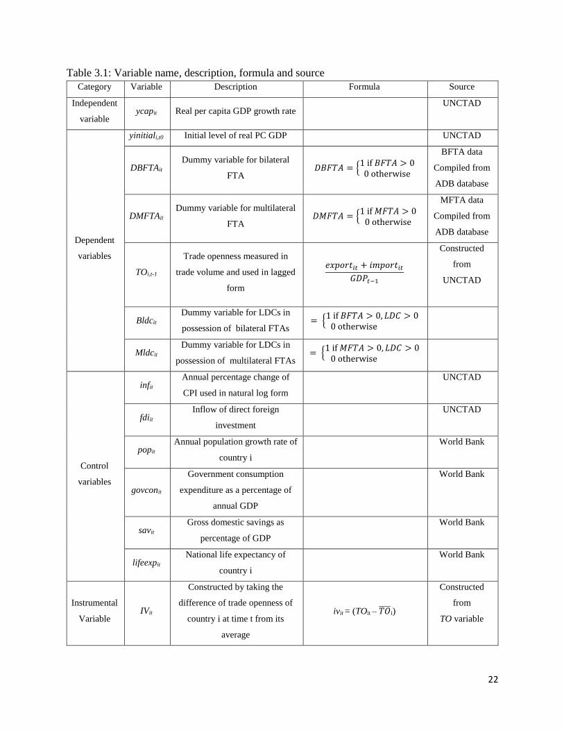
Table 3.1: Variable name, description, formula and source

Category Variable Description Formula Source

Independent

variable ycapit Real per capita GDP growth rate

UNCTAD

Dependent

variables

yinitiali,t0 Initial level of real PC GDP UNCTAD

DBFTAit

Dummy variable for bilateral

FTA 𝐷𝐵𝐹𝑇𝐴 = {

1 if 𝐵𝐹𝑇𝐴 > 00 otherwise

BFTA data

Compiled from

ADB database

DMFTAit Dummy variable for multilateral

FTA 𝐷𝑀𝐹𝑇𝐴 = {

1 if 𝑀𝐹𝑇𝐴 > 00 otherwise

MFTA data

Compiled from

ADB database

TOi,t-1

Trade openness measured in

trade volume and used in lagged

form

𝑒𝑥𝑝𝑜𝑟𝑡𝑖𝑡 + 𝑖𝑚𝑝𝑜𝑟𝑡𝑖𝑡

𝐺𝐷𝑃𝑡−1

Constructed

from

UNCTAD

Bldcit Dummy variable for LDCs in

possession of bilateral FTAs = {

1 if 𝐵𝐹𝑇𝐴 > 0, 𝐿𝐷𝐶 > 00 otherwise

Mldcit Dummy variable for LDCs in

possession of multilateral FTAs = {

1 if 𝑀𝐹𝑇𝐴 > 0, 𝐿𝐷𝐶 > 00 otherwise

Control

variables

infit Annual percentage change of

CPI used in natural log form

UNCTAD

fdiit Inflow of direct foreign

investment

UNCTAD

popit Annual population growth rate of

country i

World Bank

govconit

Government consumption

expenditure as a percentage of

annual GDP

World Bank

savit Gross domestic savings as

percentage of GDP

World Bank

lifeexpit National life expectancy of

country i

World Bank

Instrumental

Variable IVit

Constructed by taking the

difference of trade openness of

country i at time t from its

average

ivit = (TOit – 𝑇𝑂̅̅ ̅̅ i)

Constructed

from

TO variable

23

Detailed explanation of every variable and their construction methods are presented in the

following section.

3.2.1 Dependent Variables

ycapit is the dependent variable representing the annual average per capital GDP growth rate of

country i at time t at constant national currency. Contemporaneous literatures have used it as an

indicator to describe the pace of economic development of an economy.

3.2.2 Independent Variables

yinitiali,t0 is initial level of real per capital GDP in the OLS benchmark regressions. Dollar and

Kraay (2004) used such per capital GDP levels to account for the initial state as suggested by the

neoclassical growth theory. This variable takes into account the per capita GDP of the year one of

the data timeline for each country i. The variable is expected to exhibit negative sign in keeping

with the growth theories.

ycapi,t-1 is a lagged value of the dependent variable ycap. The crucial assumption of Arellano-Bond

estimate of the dynamic panel model is that the current dependent variable is influenced by its past

form. Previous economic literatures have shown that past growth levels of per capita GDP growth

can influence current growth level. This convergence is tasted with the inclusion of initial GDP

per capita. The lagged dependent variable serves as a proxy for the initial GDP variable.

DBFTAit is the dummy variable which takes the value of 1 for country i for any positive number

of in effect bilateral FTA at t year and 0 otherwise. Talking inspiration from the past literature to

capture the effect of FTA on economic development the dummy variable DBFTA is created. The

dummy variable is created based on the variable BFTA which symbolizing the number of

concluded and in effect bilateral FTAs for country i at time t.

DMFTAit is the dummy variable which takes the value of 1 for country i for any positive number

of in effect multilateral FTA at t year and 0 otherwise. To capture the effect of FTA on economic

development the dummy variable DMFTA is created. The dummy variable is created based on the

variable MFTA which symbolizing the number of concluded and in effect Multilateral FTAs for

country i at time t.

24

TOit is the variable describing the trade openness of a country. A trade volume index approach is

used to measure the trade openness. This index, as provided by the World Bank and used in a

multitude of studies, is defined as the simple ratio of exports and imports to the GDP level of a

country. Many acknowledged studies have used and proved the validity of this approach through

significance; Frankel and Romer (1999), Dollar and Kraay (2004) among others. A modified form

of the ratio, which includes the one-year lag of the GDP level is used in this research. The

approach, first mentioned by Koeniger and Busse (2012), appears to be reasonable as it tackles the

issue that the trade to GDP ratio in its standard form can conceal important information, in that an

increase in exports and imports, e.g., leads to a concurrent increase of the GDP of a country.

Koeniger and Busse state “This trade measure avoids a potential bias due to simultaneous changes

of both the nominator, volume of exports and imports, and the denominator, total GDP.” Lastly,

the trade openness variable itself is used in lagged form, TOi,t-1 ;following Dollar and Kraay (2004)

and Gries and Redlin (2012). This solves one endogeneity problem of potential reverse causality

between the explanatory variable TOi,t-1 and the dependent variable ycapit.

infit is the annual percentage change in the cost of acquiring a basket of services and goods for

average consumer that may be fixed or changed at specified intervals on yearly basis, as measured

by CPI. The inflation rate serves as proxy for financial stability or monetary policy of a country.

The data is converted into percentage points and the natural logarithm form of the variable is used

for the study.

fdiit stands for the inflow of foreign direct investment for country i at t year. The inflow is measured

as flow of direct foreign investment rather than stock. The fdi is taken as an annual percentage of

GDP.

popit stands for annual growth of total population for country i. The idea is to use it as a proxy for

the labour force growth of a country. Dollar and Kraay (2004) include this as growth rate.

Yanikkaya (2003) uses population densities in his growth regression. This paper uses the annual

population growth rate.

govconit stands for all government final consumption expenditures for purchases of goods and

services (including compensation of employees) and is evaluated as ratio to real GDP. Barro

(1991); Folster and Henrekson (2001) used government consumption expenditure in their work as

a measure of growth. As a macro variable researchers have used both lagged and non-lagged

25

version government consumption. This research uses a non-lagged version of the variable. The

government consumption to GDP ratio proxies for institutional stability of a country.

savit represents the gross domestic savings rate for a country. It is measured as the total domestic

savings less final consumption expenditure (total consumption) as a percentage of GDP. Osang

and Pereira (1997) used savings to examine growth rate with respect to trade volumes. Savings

serve as a proxy for economic stability of a country.

lifeexpit represents the number of years a newborn infant would live if prevailing patterns of

mortality at the time of its birth were to stay the same throughout its life. Yanikkaya (2003)

includes 5 year lagged value of life expectancy to capture its effect on growth. In this paper non

lagged value of life expectancy has been used.

Bldcit is the dummy variable for least developed countries in possession of in effect bilateral FTAs.

This dummy variables characterizes the effect of bilateral FTAs for a LDC member on its growth.

It takes a value of 1 for a LDC country having any number of positive in effect bilateral FTAs at

year t and 0 otherwise. The dummy variable is created based on the interaction between BDFTA

and LDC variable.

Mldcit is the dummy variable for least developed countries in possession of in effect multilateral

FTAs. This dummy variables characterizes the effect of multilateral FTAs for a LDC member on

its growth. It takes a value of 1 for a LDC country having any number of positive in effect

multilateral FTAs at year t and 0 otherwise. The dummy variable is created based on the interaction

between DMFTA and LDC variable.

3.2.3 Instrumental Variables

Apart from the lags of the dependent and the independent variables the following variable is also

used as an instrumental variable for the dynamic panel model.

IVit is the instrumental variable used for the trade openness variable where account is given to the

potential endogeneity of the open variable. For the construction of the instrumental variable the

average of trade openness for each country over the entire period from 1990 to 2013 was built.

Then a new series for the instrumental variable is calculated for each country i by differencing the

observation of the trade volume variable and its average, such that:

26

ivit = (xit – �̅�i) (3.4)

The construction of instrumental variable are inspired by Dollar and Kraay (2004) and supported

and described in Verbeek (2012).

This instrumental variable approach is superior than that of studies reviewed by Harrison and

Rodríguez (2009). They use geographical distance as an instrument variable with a gravity model.

This is a weak approach as geographical distance does not change over time and its assumption

also does not hold under real world settings. This approach assumes countries trade more through

shared borders. In reality Asian countries exhibits higher inter region trade than intra region. For

instance, Bangladesh exports approx. more than 87% of its total exports to USA an EU compared

to Asian countries.

3.2.4 Selection of Variables

According to past literature initial level of real GDP per capita, investment share of GDP, measure

of human capital such as school enrolment rate and population growth explain approx. half of the

cross section variance of growth rates. This also serves as inspiration for the variables selected in

this research.

The yinitiali,t0 variable has been used in the OLS regressions to test the convergence of the steady

state as predicted by the neoclassical growth theory and to maintain competency with the past

literature.

The data for domestic invest share of GDP of the subject counties is inadequate. The author

includes FDI share of GDP and domestic savings share of GDP to account for this phenomena.

For the measure of human capital primary school enrolment rate were included in the regression

models. Unfortunately, when tested the variable exhibited contradictory sign and significance to

that of economic theory and past literature. The preference of the variable resulted in an enormous

drop in the Wald chi2 statistics. The results remained unchanged even after testing the variable

from two different data bases, the World Bank and UNESCO respectively. Therefore, it was

decided to drop the variable from the data set as the author aims to secure non-biased estimations.

Population growth rate is included in this study as claimed by the past literature.

27

The first significance portion of residuals is explained by economic indicators such as political

stability and market distortions etc., according to past studies. The author tried to include rule of

law and government efficiency to account for such indicators. Unfortunately, the availability of

data has been an obstacle in this case. Both of the data set suffer from nine missing values for each

of the subject countries in the time period of the study including starting seven years of the time

period. An interpolation could have been done. However, as starting seven values were missing

rather than values in the middle of the time line; the fitted values would result in biased and low

precision estimations. Therefore, the author decided not to include this variables.

The second portion of the residual is explained by international factors which is the central focus

of this research. The study includes trade openness and dummy variables for FTAs to examine the

impact of trade variables on growth rate.

3.3 Data

3.3.1 Data Timeline

The study is focused on the Asia region. The Asian countries have shown tremendous economic

development in recent years. The study takes into account 31 Asian countries after dropping some

outliers with large gap in their data. The time line of the data is 24 years staring from 1990 to 2013.

The past studies on trade openness have larger timeline; however, as the paper focuses on impact

of FTA and they only came into the trade scenario of Asia during 1990s, a later starting point for

the data set is selected. Before 1990 the number of in effect FTAs in Asia were almost nonexistent.

Nominal number of the subject countries of this study had positive number of in effect FTA in

1990. The notion of FTA gradually appeared for the Asian countries in 1990s and picked up the

pace in the 2000s. The end period is 2013 as the data for many subject countries for the year 2014

has not been published yet. Therefore, 1990-2013 is considered the proper timeline for the research

which lets the paper take into account recent data for the variables. After dropping outlier the final

dataset provides a strongly balanced dynamic panel dataset.

Majority of the countries have experienced positive growth in per capita GDP during the study

time period. The decadal average of 1990s and 2000s (Appendix) show greater increase in per

capita GDP growth in the 2000s compared to that of 1990s. Many of the countries actually doubled

28

their growth rate of GDP/capita. The graph of trade openness index (Appendix) also exhibits

increased openness of the economies during the data time line, with different dimensions.

3.3.2 Data Sources

The dataset used in this paper is compiled from several sources. The FTA data is collected from

the ADB ARIC database which provides information on country-wise FTAs. The data for GDP

per capita growth rate, real PC GDP level, trade volume, annual GDP, FDI, inflation is obtained

from United Nations Conference of Trade and Development (UNCTAD) statistics data base. The

savings, annual population growth rate, life expectancy and government consumption expenditure

data has been secured from World Development Indicator of the World Bank database.

4. Hypotheses

4.1 FTAs and Asia

The Asian countries have also realized the importance of regional integration. The Asian countries

have two regional associations; South Asian Association for Regional Corporation (SAARC) and

Association of Southeast Asian Nations (ASEAN). SAARC founded in 1985 has eight member

countries - Afghanistan, Bangladesh, Bhutan, India, Maldives, Nepal, Pakistan, and Sri Lanka. In

2006, SAARC launched the South Asian Free Trade Area (SAFTA) for its member countries.

Following the launch of the FTA the intra-SAARC exports increased substantially to $354.6

billion in 2012 from $206.7 billion in 2009.

ASEAN, founded in 1967 is greater of the two regional organizations. It started with five then

extended to ten member countries – Brunei, Cambodia, Indonesia, Laos, Malaysia, Myanmar,

Philippines, Singapore, Thailand, and Vietnam. ASEAN realizing the importance of regional

integration expanded to include China, Japan and South Korea, three major economies of Asia is

now known as ASEAN plus three. ASEAN launch the ASEAN Free Trade Agreement (AFTA) in

1992. Apart from the AFTA, ASEAN has FTAs with China, Korea, Japan, Australia, New

Zealand, and India. The expected bilateral trade between ASEAN and China alone for 2015 was

$500 billion.

The following table presents the number of concluded and in effect FTAs both bilateral and

multilateral as of 2015 for the subject countries of this particular study.

29

Table 4.1: In effect FTAs as of 2015

Source: compiled from ADB ARIC database

Country Bilateral FTAs Multi-lateral FTAs Total FTAs

Armenia 8 2 10

Azerbaijan 4 1 5

Bangladesh 0 3 3

Bhutan 1 1 2

Brunei Darussalam 1 7 8

Cambodia 0 6 6

China 14 2 16

Fiji 0 3 3

Georgia 8 3 11

Hong Kong 3 1 4

India 9 4 13

Indonesia 2 7 9

Iran 2 0 2

Japan 13 1 14

Korea [republic of] 11 4 15

Kyrgyz 7 2 9

Lao PDR 1 7 8

Malaysia 7 7 14

Maldives 0 1 1

Myanmar 0 6 6

Nepal 1 1 2

Pakistan 7 3 10

Philippines 1 6 7

Saudi Arabia 0 2 2

Singapore 11 9 20

Sri Lanka 3 2 5

Tajikistan 6 1 7

Thailand 7 6 13

UAE 0 2 2

Vietnam 3 6 9

Yemen 0 1 1

30

Among the countries Singapore is in the lead with 20 FTAs, followed by China with 16 and South

Korea with 15 FTAs. The leading Asian economies are making haste in securing greater number

of FTAs with their trading partners. Currently China, India, South Korea and Singapore have

7,15,8 and 8 FTAs under negotiations respectively. Asia trumps Americas’ in FTAs per country.

On average Asia has 3.8 concluded FTAs per country compared with 2.9 for the America’s. Rapid

rise in the number of FTAs among the Asian countries point in the direction that the FTAs are

believed to be instrumental in the growth of the economy.

The target of this research is to investigate the effect of FTAs on economic growth. The effect of

the FTAs that are in negotiation phase or have been signed but have not been called into force are

difficult to demonstrate. Therefore, to capture the distinguish effect the study only considers the

FTAs which have been signed and put into effect by the member countries. The leading economies

of Asia such as China, India, Japan, South Korea and Singapore have significantly greater number

of bilateral FTAs compared to those of their multilateral FTAs. It is assumed by the policy makers

that since the number of interested parties in bilateral FTAs is generally restricted to two, it

provides the member countries a greater negotiations power in the trade deal. There is less conflict

of interest when compared to dealing with a trade bloc or cluster of countries and it is assumed to

be more effective in terms of economic growth due to the favorable trade conditions of the member

countries. Hence the first hypothesis tested in the paper is:

Hypothesis 1: Bilateral FTAs have a positive and significant effect on the economic growth of its

member countries

The first regression model of the paper is:

Past literature mostly considered the effect of bilateral FTAs. Despite being lower in number to

the bilateral FTAs there are significant number of in effect multilateral FTAs for the Asian

countries. Regardless of being the more complicated version of the FTAs to negotiate the

multilateral FTAs are able to provide access to vast trade areas. With an aim to scrutinize the effect

of FTAs on economic growth, this research examines the bilateral and multilateral FTAs

separately. This adds a new dimension to the existing literature.

Δycapit= γΔycapi(t−1) +β1ΔDBFTAit + β2ΔXit +Δεit (4.1)

31

The second hypothesis is:

Hypothesis 2: Multilateral FTAs have a positive and significant effect on the economic growth of

its member countries

The second regression model of the paper-

4.2 Openness of Asia

The Asian economies are becoming more trade orientated and thus more open. In 2013, 5% of

world imports and 10% of world’s commercial services exports are attributed to ASEAN. In 2014,

ASEAN shipped 7% of total world merchandise exports. Asia as a region is the second biggest

exporter and importer in world merchandise trade after Europe. China and Japan hold the first and

the fourth position for global export of merchandise in 2014. The following figure demonstrates

the share of Asia as a region in the world merchandise trade.

Figure 4.1: Asia’s share of world merchandise trade

Source: International Trade Statistics 2015

19.1

26 26.1

32

18.5

23.5 23.5

31.5

0

5

10

15

20

25

30

35

1983 1993 2003 2013

% o

f W

orl

d T

rad

e

export import

Δycapit= γΔycapi(t−1) +β1ΔDMFTAit + β2ΔXit +Δεit (4.2)

32

It is apparent from the chart that Asia’s share in the world trade is increasing. This upward

movement started in the latter part of the last century. Asia has been blessed with vast workforce

and the Asian economies have been intelligent to utilize their massive workforce to turn their

economies into manufacture economies. This openness nature of the Asian economies is greatly

attributed to the FTAs, both bilateral and Multilateral. The FTAs generally ensure nominal to zero

tariff on imports for a member country in the market of its FTA-partner country. This has been

instrumental in increasing the competitiveness of the emerging Asian economies and fueling the

export boom of the region. However, there is another side of this phenomenon. The developing

and LDCs of Asia are net importers. The bulk portion of raw materials and intermediate goods of

their export industries are imported. FTAs work as a balancing force to facilitate the Asian

countries. This leads the author to suspect that without the presence of FTAs, individually trade

openness would actually deter economic growth of a country. Therefore, the third hypothesis for

the paper is:

Hypothesis 3: Trade openness in absence of FTAs has a negative and significant effect on the

economic growth a country

The regression model for testing trade openness is the following:

4.3 FTA and openness

FTA and trade openness are anticipated to have an effect on economic growth independently.

Nonetheless, there is a relatively new notion of the “third country”. It is suspected that having an

FTA may induce one of the member countries to trade in greater proportion than earlier with a

third country who does not belong to the FTA group. One economic intuition to this scenario is

forming an FTA leads to grater trade volume between the member countries. The increased amount

of trade demands higher raw materials and intermediate goods for the finished products. This could

lead to the member countries trading in increased volume with a third country despite being a non-

FTA country which in turn makes the member countries economy more open. Chen and Joshi

(2010) showed that the third country effects play an important role in countries' decision to

establish new FTAs. The FTAs aims to ensure that there is no exploitation in the trade dimension

Δycapit= γΔycapi(t−1) +β1ΔTOi,t-1 + β2ΔXit +Δεit (4.3)

33

by creating a win-win situation for the interested parties and creating an indirect positive

externality. Trade openness with non-FTA partners in a controlled measure, coupled with FTAs is

expected to result in positive economic growth. Thus the hypotheses becomes:

Hypothesis 4: Bilateral FTAs in the presence of trade openness has a positive and significant effect

on a country’s economic growth

Regression model to test the hypothesis regarding bilateral FTA and trade openness is-

To scrutinize the effects of bilateral and multilateral FTAs separately the next hypothesis is-

Hypothesis 5: Multilateral FTAs in the presence of trade openness has a positive and significant

effect on a country’s economic growth

Regression model to test the hypothesis regarding multilateral FTA and trade openness is-

4.4 Growth of Least Developed Countries

There are nine LDCs in Asia. Afghanistan, Bangladesh, Bhutan, Cambodia, East Timor, Laos,

Myanmar, Nepal and Yemen. Unfortunately, East Timor doesn’t have any sort of FTA and

Afghanistan lack adequate data to run statistical tests. The paper considers the rest of the seven

countries as subject for this research. The LDC countries of Asia are heavily export oriented. In

2010, the ratio of total export of goods and services to GDP for Bangladesh, Bhutan, Cambodia,

Laos, Myanmar, Nepal and Yemen was 19.4, 37.1, 52.1, 31.1, 15.5, 9.3 and 39.7 respectively.

According to growth theories the Least Developed Countries (LDC) experience higher degree of

growth compared to the developed economies for the same degree of growth measures for being

at the initial phase of the growth path. This statement is also holds for negative effects. Researchers

suspect opening up the economies of the LDCs by eliminating all protective trade barriers can

reduce the net national income. Clemens and Williamson (2001), found a positive correlation

between import tariffs and economic growth across countries during the late nineteenth century.

Δycapit = γΔycapi(t−1) +β1ΔDBFTAit + β2ΔTOi,t-1 + β3ΔXit +Δεit (4.4)

Δycapit = γΔycapi(t−1) +β1ΔDMFTAit + β2ΔTOi,t-1 + β3ΔXit +Δεit (4.5)

34

Among the Asian LDCs Bangladesh, Cambodia, Myanmar and Yemen doesn’t have any bilateral

FTAs. The LDCs lack the socio-economic position to influence terms of trade in their favor in the

FTA negotiations. A bilateral FTA with LDCs are sometimes considered a liability by the

developed counterparts. Oskooee, Mohtadi, and Shabsigh (1991) found negative relation between

export growth and economic growth of Indonesia. Abbas (2014) found negative effect of trade

liberalization index on economic growth of LDCs. This paper suspects a negative relation with the

FTAs and the growth of the LDCs. The paper tests the effect of FTA on LDCs by introducing a

dummy variable. The hypothesis is:

Hypothesis 6: There is significant negative difference on the effect of Bilateral FTAs on growth of

the least developed countries

The regression equation:

Then the effect of bilateral FTAs on LDCs are tested in the presence of trade openness. The LDCs

have implemented protective measures for their domestic industries. However, the author suspects

even with established protection policies the LDCs experience a negative effect on growth due to

the FTAs.

Hypothesis 7: There is significant negative difference on the effect of Bilateral FTAs even in the

presence of trade openness on growth of the least developed countries

The regression equation:

The paper examines the effects of bilateral and multilateral FTAs independently. The last two

hypotheses of the author’s work is to scrutinize the effects of multilateral FTAs on economic

growth of LDCs. A negative relation is also suspected in case of the multilateral FTAs due to

similar underlying assumptions. The hypothesis is:

Hypothesis 8: There is significant negative difference on the effect of Multilateral FTAs on growth

of the least developed countries

Δycapit= γΔycapi(t−1) +β1ΔBldcit + β2ΔXit +Δεit (4.6)

Δycapit= γΔycapi(t−1) +β1ΔBldcit + β2ΔTOi,t-1 + β3ΔXit +Δεit (4.7)

35

The regression model:

Lastly, author suspects even with trade openness the LDCs experience a negative effect on growth

due to the multilateral FTAs. The final hypothesis of the paper is:

Hypothesis 9: There is significant negative difference on the effect of Multilateral FTAs even in

the presence of trade openness on growth of the least developed countries

The last regression model in this paper to be tested is-

5. Empirical Outputs

The outputs of the estimated regressions along with their interpretation are presented are presented

in this section.

5.1 Unit root tests

The analysis begins with testing the core variables for unit roots. Presence of unit root in a variable

may lead to spurious regression results. The dependent variable ycapit and the independent variable

TO are tested for unit roots. The FTAs enter the regression models as dummy variables which

doesn’t contain unit roots by construction. The Augmented Dickey-Fuller (ADF) test has been

used for unit roots.

The dependent variable ycapit doesn’t contain unit roots when tested by ADF including time trend

and one lagged difference. The inverse chi-square and modified inverse chi-square both are highly

statistically significant with p-values of 0.0000 which allows us to reject the null hypothesis of “all

panel contains unit root”.

Table 5.1: Unit root test of ycapit

Statistic p-value

Inverse chi-squared(62) P 219.2998 0.00

Inverse normal Z -8.8556 0.00

Inverse logit t(159) L* -10.1958 0.00

Modified inv. chi-squared Pm 14.1259 0.00

Δycapit= γΔycapi(t−1) +β1ΔMldcit + β2ΔXit +Δεit (4.8)

Δycapit= γΔycapi(t−1) +β1ΔMldcit + β2ΔTOi,t-1 + β3ΔXit +Δεit (4.9)

36

Next, the TOit variable is tested for unit roots with the ADF test. The TOit variable does contain

unit roots. However, for this research the lagged version of TO have been used. When TOi,t-1 is

tested for unit roots with the ADF approach it does not exhibit any unit roots. This secures the

research from coming across spurious regression results. The inverse chi-square and modified

inverse chi-square both are highly statistically significant with p-values of 0.0000 which allows us

to reject the null hypothesis of “all panel contains unit root”.

Table 5.2: Unit root test of TOi,t-1

Statistic p-value

Inverse chi-squared(62) P 505.1444 0.00

Inverse normal Z -8.0423 0.00

Inverse logit t(159) L* -21.4350 0.00

Modified inv. chi-squared Pm 39.7955 0.00

5.2 Hypotheses Estimations

The dynamic panel models are estimated by the Arellano-Bond approach which corrects for the

unobservable endogeneity and heteroskedasticity by using lags of dependent and independent

variable created with GMM type moments as instrumental variables. In the regression models with

trade openness an additional instrumental variable IV has been used along with the differentiated

instrumental variables used in the Arellano-Bond approach.

5.2.1 Hypothesis 1

The first hypothesis tests the effect of bilateral FTAs on a country’s economic growth. First a

simple OLS model has been run with the dependent variable, the dummy variable of bilateral FTAs

and the initial level per capita GDP. A second OLS regression has been run including all the

control variables. These two models are used as benchmarks to compare the results with the

Arellano-Bond models.

In the first OLS model DBFTAit is positive in value. It changes sign to negative in presence of the

control variables. It is statistically insignificant in both of the equations. The yinitiali,t0 variable is

high statistical significance with negative sign in both equations confirming the assumption of

neoclassical growth theory. The control variables inflation, population growth, domestic savings

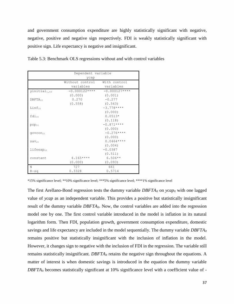
37

and government consumption expenditure are highly statistically significant with negative,

negative, positive and negative sign respectively. FDI is weakly statistically significant with

positive sign. Life expectancy is negative and insignificant.

Table 5.3: Benchmark OLS regressions without and with control variables

*15% significance level; **10% significance level; ***5% significance level; ****1% significance level

The first Arellano-Bond regression tests the dummy variable DBFTAit on ycapit with one lagged

value of ycap as an independent variable. This provides a positive but statistically insignificant

result of the dummy variable DBFTAit. Now, the control variables are added into the regression

model one by one. The first control variable introduced in the model is inflation in its natural

logarithm form. Then FDI, population growth, government consumption expenditure, domestic

savings and life expectancy are included in the model sequentially. The dummy variable DBFTAit

remains positive but statistically insignificant with the inclusion of inflation in the model.

However, it changes sign to negative with the inclusion of FDI in the regression. The variable still

remains statistically insignificant. DBFTAit retains the negative sign throughout the equations. A

matter of interest is when domestic savings is introduced in the equation the dummy variable

DBFTAit becomes statistically significant at 10% significance level with a coefficient value of -

Dependent variable

ycap

Without control

variables

With control

variables

yinitiali,t0 -0.000122**** -0.000127****

(0.000) (0.001)

DBFTAit 0.270 -0.277

(0.558) (0.543)

Linfit -3.778****

(0.000)

fdiit 0.0513*

(0.118)

popit -0.871****

(0.000)

govconit -0.276****

(0.000)

savit 0.0464****

(0.004)

lifeexpit -0.0387

(0.511)

constant 4.165**** 6.506**

(0.000) (0.093)

N 727 661

R-sq 0.3328 0.5714

38

1.185. This finding is contradictory to the hypothesis. With the inclusion of the last control variable

life expectancy, the dummy variable DBFTAit again becomes statistically insignificant while

retaining the negative sign.

Table 5.4: Arellano-Bond estimations of the first hypothesis


All Wald chi2 statistics are statistically significant with 0.000 p-values

Dependent variable

ycap

(1) (2) (3) (4) (5) (6) (7)

ycapi,t-1 0.455**** 0.411**** 0.412**** 0.406**** 0.412**** 0.394**** 0.393****

(0.000) (0.000) (0.000) (0.000) (0.000) (0.000) (0.000)

DBFTAit 0.315 0.0163 -0.0786 -0.409 -0.577 -1.185** -0.504

(0.631) (0.981) (0.907) (0.545) (0.349) (0.069) (0.530)

Linfit -1.222**** -1.127**** -1.216**** -1.300**** -1.210**** -1.373****

(0.004) (0.008) (0.004) (0.001) (0.002) (0.001)

fdiit 0.0793** 0.0881*** 0.0690** 0.0765** 0.0787***

(0.063) (0.039) (0.080) (0.054) (0.048)

popit -0.683**** -0.868**** -0.814**** -0.815****

(0.001) (0.000) (0.000) (0.000)

govconit -0.424**** -0.409**** -0.387****

(0.000) (0.000) (0.000)

savit 0.0665**** 0.0756****

(0.008) (0.003)

lifeexpit -0.164*

(0.150)

constant 1.915**** 0.830* 0.648 1.769**** 7.363**** 5.888**** 16.37***

(0.000) (0.117) (0.229) (0.005) (0.000) (0.000) (0.028)

N 663 649 649 649 610 601 601

Wald chi2 191.33 205.50 209.18 220.72 326.54 335.61 338.75

39

The lagged value of per capita GDP growth rate is positive and highly statistically significant in

all estimations. Proving the assumption that the present growth rate of PC GDP growth is highly

influence by past growth rates.

Inflation is highly statistically significant throughout the models with a negative sign. This is

intuitive as higher level of inflation lower the growth rate of per capita GDP. FDI is positive and

statistically significant in all models. This is supported by economics theories as more inflow of

FDI leads to greater economic activities which enhances the growth rate of per capita GDP.

Population growth rate is highly statistically significant throughout the models with a negative

sign. Asia has few of the most densely populated countries such as Bangladesh, China and India

which accounts for one third of the world population. Higher population growth leads to

exhaustion of resources and high level of poverty which slows down economic growth.

Government consumption expenditure is negatively statistically significant. Past research has

found higher government expenditure leads to lower growth of economy (Barro (1991)). Domestic

savings is positive and highly statistically significant. Higher rate of savings implies higher level

of per capita income. Lastly, life expectancy is weakly statistically significant with a negative sign.

Higher life expectancy implies a greater number of senior population who depend on government

in terms of pension. This leads to supplementary pressure on limited resources and lower economic

growth, a situation currently faced by Japan.

The results of these regression equation leads to the conclusion that bilateral FTA does not exhibit

positive and significant influence on country’s economic growth. The first hypothesis is rejected.

5.2.2 Hypothesis 2

The second hypothesis tests the effect of multilateral FTAs on a country’s economic growth. First

two simple OLS model has been run. First OLS models tests the dependent variable ycapit, the

dummy variable of multilateral FTAs and yinitiali,t0. Second OLS regression has been tested

including all the control variables. These two models are used as benchmarks to compare the

results with the Arellano-Bond models.

40


Dependent variable

ycap

Without control

variables

With control

variables

yinitiali,t0 -0.000124**** -0.000129****

(0.000) (0.001)

DMFTAit 0.191 -0.862**

(0.695) (0.059)

Linfit -3.835****

(0.000)

fdiit 0.0491*

(0.134)

popit -0.834****

(0.000)

govconit -0.286****

(0.000)

savit 0.0502****

(0.002)

lifeexpit -0.0357

(0.508)

constant 4.173**** 6.633**

(0.000) (0.065)

N 727 661

R-sq 0.3434 0.5747


The dummy variable for multilateral FTAs, DMFTAit is positive in the first OLS model.

Fascinatingly, it turns negative and gains statistical significance in the second OLS equation. The

initial level per capita GDP is highly statistically significant at 1% significance level in both OLS

models. Every control variables are statistically significant in different level of significance with

expected signs excluding lifeexpit.

Now, the dynamic panel models are estimated. The first Arellano-Bond regression tests the dummy

variable DMFTAit on ycapit with one lag of ycapi,t-1 as an independent variable. The lagged version

of real per capita GDP growth rate which represents a proxy for initial GDP in this research, is

highly statistically significant at 1% significance level with p-value of 0.000 in all the estimations.

This is in line with economic theories, implicating that past values of growth rate can influence

the growth rate of the present.

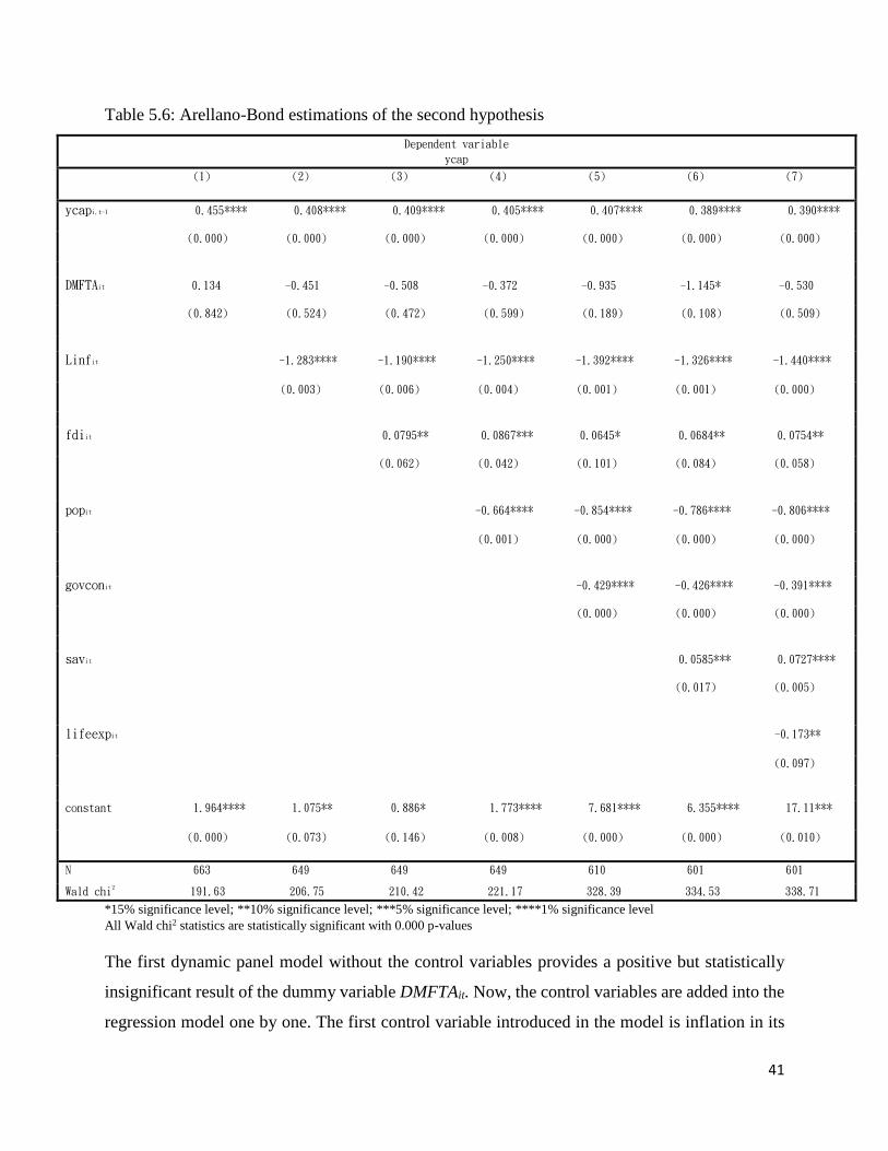
41

Table 5.6: Arellano-Bond estimations of the second hypothesis

Dependent variable

ycap

(1) (2) (3) (4) (5) (6) (7)

ycapi,t-1 0.455**** 0.408**** 0.409**** 0.405**** 0.407**** 0.389**** 0.390****

(0.000) (0.000) (0.000) (0.000) (0.000) (0.000) (0.000)

DMFTAit 0.134 -0.451 -0.508 -0.372 -0.935 -1.145* -0.530

(0.842) (0.524) (0.472) (0.599) (0.189) (0.108) (0.509)

Linfit -1.283**** -1.190**** -1.250**** -1.392**** -1.326**** -1.440****

(0.003) (0.006) (0.004) (0.001) (0.001) (0.000)

fdiit 0.0795** 0.0867*** 0.0645* 0.0684** 0.0754**

(0.062) (0.042) (0.101) (0.084) (0.058)

popit -0.664**** -0.854**** -0.786**** -0.806****

(0.001) (0.000) (0.000) (0.000)

govconit -0.429**** -0.426**** -0.391****

(0.000) (0.000) (0.000)

savit 0.0585*** 0.0727****

(0.017) (0.005)

lifeexpit -0.173**

(0.097)

constant 1.964**** 1.075** 0.886* 1.773**** 7.681**** 6.355**** 17.11***

(0.000) (0.073) (0.146) (0.008) (0.000) (0.000) (0.010)

N 663 649 649 649 610 601 601

Wald chi2 191.63 206.75 210.42 221.17 328.39 334.53 338.71



The first dynamic panel model without the control variables provides a positive but statistically

insignificant result of the dummy variable DMFTAit. Now, the control variables are added into the

regression model one by one. The first control variable introduced in the model is inflation in its

42

natural logarithm form. Then FDI, population growth, government consumption expenditure,

domestic savings and life expectancy are incorporated in the regressions sequentially. With

inclusion of first control variavble infit the dummy variable DMFTAit changes its sign to negative

but remains statistically insignificant with the inclusion of inflation in the model. DMFTAit retains

the negative sign throughout the equations. A matter of interest is when domestic savings is

introduced in the equation the dummy variable DMFTAit becomes statistically significant at 15%

significance level with a coefficient value of -1.145. This shows multilateral FTAs actually have

a negative effect on economic growths of its member countries. This finding is contradictory to

the hypothesis. With the inclusion of the last control variable life expectancy, the dummy variable

DMFTAit again becomes statistically insignificant while retaining the negative sign.

The control variable inflation is highly statistically significant throughout each models with a

negative sign. FDI is positively statistically significant in all models. Population growth rate is

highly statistically significant throughout the models with a negative sign. Government

consumption expenditure is negatively statistically significant. Domestic savings is positive and

highly statistically significant. Higher rate of savings implies higher level of per capita income.

Lastly, life expectancy is weakly statistically significant with a negative sign. All of them exhibit

expected signs and follow similar patterns to that of the bilateral FTA model tested earlier.

The results of these regression equations lead to the conclusion that multilateral FTAs do not

demonstrates a significant positive effect on country’s growth. The second hypothesis is rejected.

5.2.3 Hypothesis 3

The third hypothesis examines trade openness on economic growth. Contrary to popular notion

this paper suspects a negative linkage among economic growth and trade openness in the absence

of FTAs. The instrumental variable IVit has been used in the dynamic panel models.

Research begins with two benchmark OLS regressions without and with control variables

respectively. The trade openness variable in its lagged form is statistically significant and negative

in both of the models. Linfit is statistically significant and positive. All the other control variables

are statistically significant with expected signs.

43


Dependent variable

ycap

Without control

variables

With control

variables

yinitiali,t0 -0.000135**** -0.000139****

(0.000) (0.000)

TOi,t-1 -0.00671**** -0.00941****

(0.009) (0.000)

Linfit 0.388

(0.401)

fdiit 0.0723***

(0.017)

popit -0.775****

(0.000)

govconit -0.121***

(0.016)

savit 0.0845****

(0.000)

lifeexpit -0.0146

(0.783)

constant 5.431**** 7.576***

(0.000) (0.029)

N 683 622

R-sq 0.3295 0.5759


The instrument variable IVit is used in Arellano-Bond approach for these estimations. The lagged

ycapi,t-1 is highly positively statistically significant in all equations confiming the assumption of

past growth rates predicting the present growth rates of per capita GDP.

TOi,t-1 is highly tatistically significant at 1% significane level and negative both in the individual

model and in every model of the control variables. The coefficient values of TOi,t-1 increases with

inclusion of each control variable. The results proof that trade openness can actually be

deterimental for economic expansion of countries in absence of FTAs. The negative effect of trade

openness is corroborated by Grossman and Helpman (1991), Yanikkaya (2003). Both of the

literature shows countries with protection policies which leads to lower level of trade openness

experience higher growth compared to that of their counterparts. The Asian region consists of

mainly developing and LDCs. In order to achieve sustainable growth these countries require

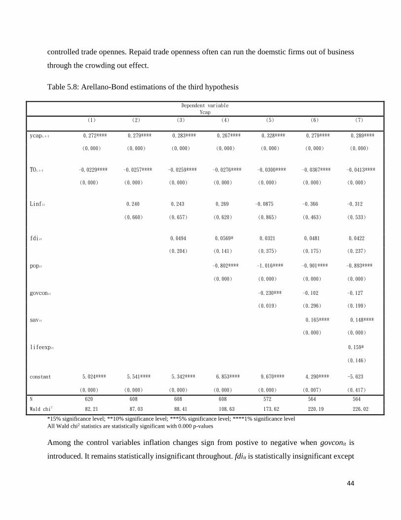
44

controlled trade opennes. Repaid trade openness often can run the doemstic firms out of business

through the crowding out effect.

Table 5.8: Arellano-Bond estimations of the third hypothesis

Dependent variable

Ycap

(1) (2) (3) (4) (5) (6) (7)

ycapi,t-1 0.272**** 0.279**** 0.283**** 0.267**** 0.328**** 0.279**** 0.289****

(0.000) (0.000) (0.000) (0.000) (0.000) (0.000) (0.000)

TOi,t-1 -0.0229**** -0.0257**** -0.0259**** -0.0276**** -0.0300**** -0.0367**** -0.0413****

(0.000) (0.000) (0.000) (0.000) (0.000) (0.000) (0.000)

Linfit 0.240 0.243 0.269 -0.0875 -0.366 -0.312

(0.660) (0.657) (0.620) (0.865) (0.463) (0.533)

fdiit 0.0494 0.0569* 0.0321 0.0481 0.0422

(0.204) (0.141) (0.375) (0.175) (0.237)

popit -0.802**** -1.016**** -0.901**** -0.893****

(0.000) (0.000) (0.000) (0.000)

govconit -0.230*** -0.102 -0.127

(0.019) (0.296) (0.199)

savit 0.165**** 0.148****

(0.000) (0.000)

lifeexpit 0.159*

(0.146)

constant 5.024**** 5.541**** 5.342**** 6.853**** 9.670**** 4.290**** -5.623

(0.000) (0.000) (0.000) (0.000) (0.000) (0.007) (0.417)

N 620 608 608 608 572 564 564

Wald chi2 82.21 87.03 88.41 108.63 173.62 220.19 226.02



Among the control variables inflation changes sign from postive to negative when govconit is

introduced. It remains statistically insignificant throughout. fdiit is statistically insignificant except

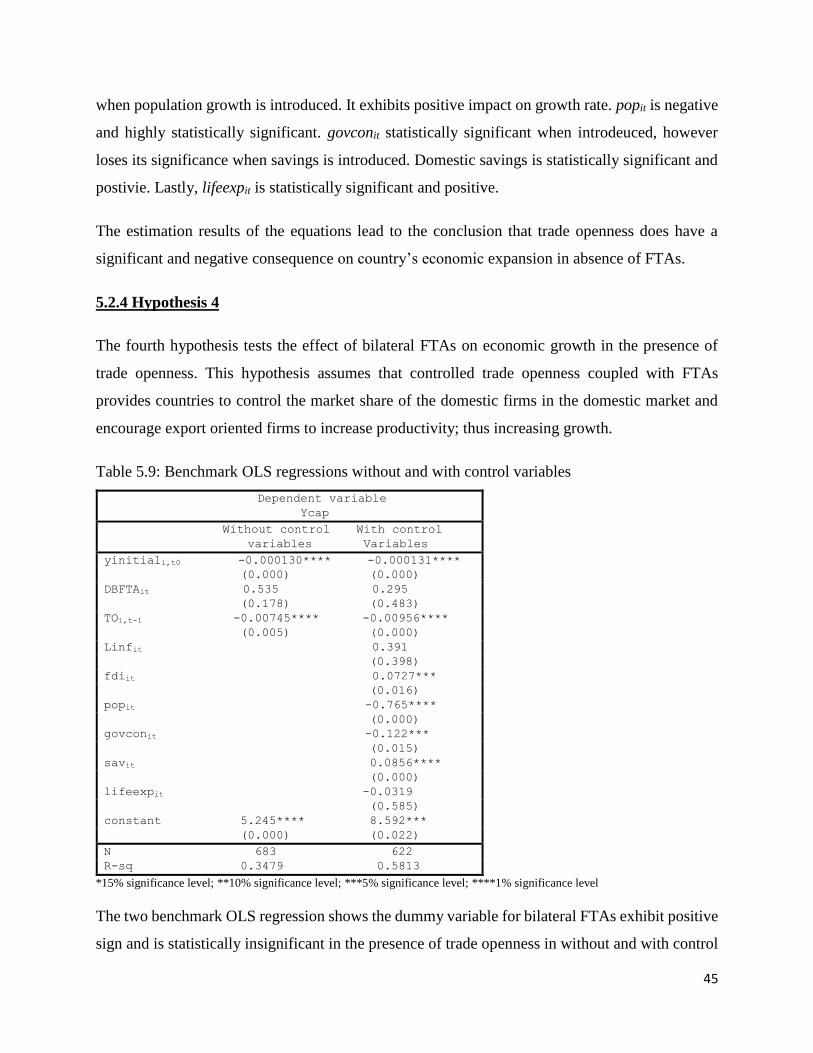
45

when population growth is introduced. It exhibits positive impact on growth rate. popit is negative

and highly statistically significant. govconit statistically significant when introdeuced, however

loses its significance when savings is introduced. Domestic savings is statistically significant and

postivie. Lastly, lifeexpit is statistically significant and positive.

The estimation results of the equations lead to the conclusion that trade openness does have a

significant and negative consequence on country’s economic expansion in absence of FTAs.

5.2.4 Hypothesis 4

The fourth hypothesis tests the effect of bilateral FTAs on economic growth in the presence of

trade openness. This hypothesis assumes that controlled trade openness coupled with FTAs

provides countries to control the market share of the domestic firms in the domestic market and

encourage export oriented firms to increase productivity; thus increasing growth.


Dependent variable

Ycap

Without control

variables

With control

Variables

yinitiali,t0 -0.000130**** -0.000131****

(0.000) (0.000)

DBFTAit 0.535 0.295

(0.178) (0.483)

TOi,t-1 -0.00745**** -0.00956****

(0.005) (0.000)

Linfit 0.391

(0.398)

fdiit 0.0727***

(0.016)

popit -0.765****

(0.000)

govconit -0.122***

(0.015)

savit 0.0856****

(0.000)

lifeexpit -0.0319

(0.585)

constant 5.245**** 8.592***

(0.000) (0.022)

N 683 622

R-sq 0.3479 0.5813


The two benchmark OLS regression shows the dummy variable for bilateral FTAs exhibit positive

sign and is statistically insignificant in the presence of trade openness in without and with control

46

variables. Trade openness still remains negative and highly statistically significant. Among the

control variables inflation and life expectancy is positive and negative respectively and both show

statistical insignificance. Other control variables are statistically significant with expected signs.

Table 5.10: Arellano-Bond estimations of the fourth hypothesis

Dependent variable

ycap

(1) (2) (3) (4) (5) (6) (7)

ycapi,t-1 0.272**** 0.278**** 0.282**** 0.267**** 0.327**** 0.281**** 0.287****

(0.000) (0.000) (0.000) (0.000) (0.000) (0.000) (0.000)

DBFTAit 2.519**** 2.360**** 2.313**** 1.982**** 1.733**** 0.814 0.504

(0.000) (0.001) (0.001) (0.004) (0.006) (0.203) (0.487)

TOi,t-1 -0.0327**** -0.0342**** -0.0342**** -0.0346**** -0.0367**** -0.0393**** -0.0417****

(0.000) (0.000) (0.000) (0.000) (0.000) (0.000) (0.000)

Linfit 0.260 0.262 0.285 -0.108 -0.363 -0.327

(0.632) (0.629) (0.598) (0.833) (0.467) (0.514)

fdiit 0.0418 0.0498 0.0239 0.0436 0.0411

(0.280) (0.196) (0.508) (0.222) (0.250)

popit -0.741**** -0.974**** -0.889**** -0.887****

(0.000) (0.000) (0.000) (0.000)

govconit -0.239*** -0.112 -0.127

(0.014) (0.250) (0.201)

savit 0.158**** 0.149****

(0.000) (0.000)

lifeexpit 0.117

(0.347)

constant 4.882**** 5.357**** 5.194**** 6.615**** 9.593**** 4.470**** -2.895

(0.000) (0.000) (0.000) (0.000) (0.000) (0.005) (0.714)

N 620 608 608 608 572 564 564

Wald chi2 97.16 99.77 100.62 117.77 182.73 222.11 226.18



In the Arellano-Bond model the instrumental variable IVit has been utilized. Lagged yacpi,t-1 is

positive and highly statistically significant in all equations. The dummy variable DBFTAit is highly

47

statistically significant at 1% significance level and positive in the presence of trade openness. It

retains its statistical significance at 1% significance level with introduction of control variables

inflation, FDI, popit and govconit. With introduction of savit into the equation it loses its statistical

significance, however remains positive in sign. One possible interpretation of this is with

increasing domestic savings there is less consumption demand in the market for both imported and

domestic products. Due to lower number of market transaction the bilateral FTAs though still

positive in value, fails to significantly affect the economic growth. In the final equation with

inclusion of lifeexpit it remains positive and statistically insignificant.

The control variables inflation, FDI and life expectancy are statistically insignificant. Population

growth is highly statistically significant in all equations. govconit is statistically significant only

when it is first introduced. savit is highly statistically significant and positive in this model.

Based on the above results it is concluded bilateral FTA can have positive impact on economic

growth in presence of trade openness if certain pre-conditions are fulfilled. Therefore, hypothesis

four cannot be rejected.

5.2.5 Hypothesis 5

The fifth hypothesis tests the effect of multilateral FTAs on economic growth in the presence of

trade openness. The paper expects to find a positive relation between multilateral FTAs and

economic growth. The instrumental variable IVit has been used in the Arellano-Bond models.

The benchmark OLS euqations show DMFTAit is negative and statistically insignificant in

presence of trade openness. Trade openness is highly statistically significant and negative in both

equations. Initial level per capital GDP exhibits negative sign as predicted. The control variables

behave in similar fashion to that of benchmark equations of the fourth hypothesis with inflation

rate and life expectancy remaining statistically insignificant.

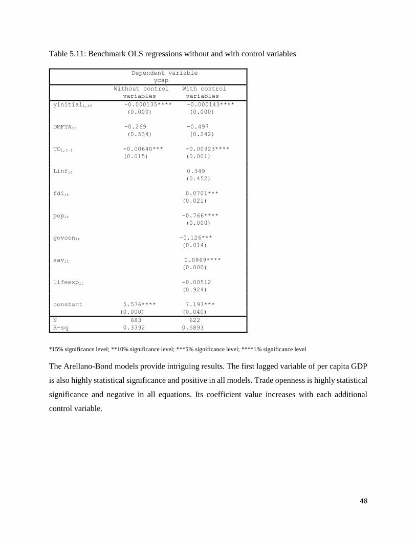
48


Dependent variable

ycap

Without control

variables

With control

variables

yinitiali,t0 -0.000135**** -0.000143****

(0.000) (0.000)

DMFTAit -0.269 -0.497

(0.534) (0.242)

TOi,t-1 -0.00640*** -0.00923****

(0.015) (0.001)

Linfit 0.349

(0.452)

fdiit 0.0701***

(0.021)

popit -0.766****

(0.000)

govconit -0.126***

(0.014)

savit 0.0869****

(0.000)

lifeexpit -0.00512

(0.924)

constant 5.576**** 7.193***

(0.000) (0.040)

N 683 622

R-sq 0.3392 0.5893


The Arellano-Bond models provide intriguing results. The first lagged variable of per capita GDP

is also highly statistical significance and positive in all models. Trade openness is highly statistical

significance and negative in all equations. Its coefficient value increases with each additional

control variable.

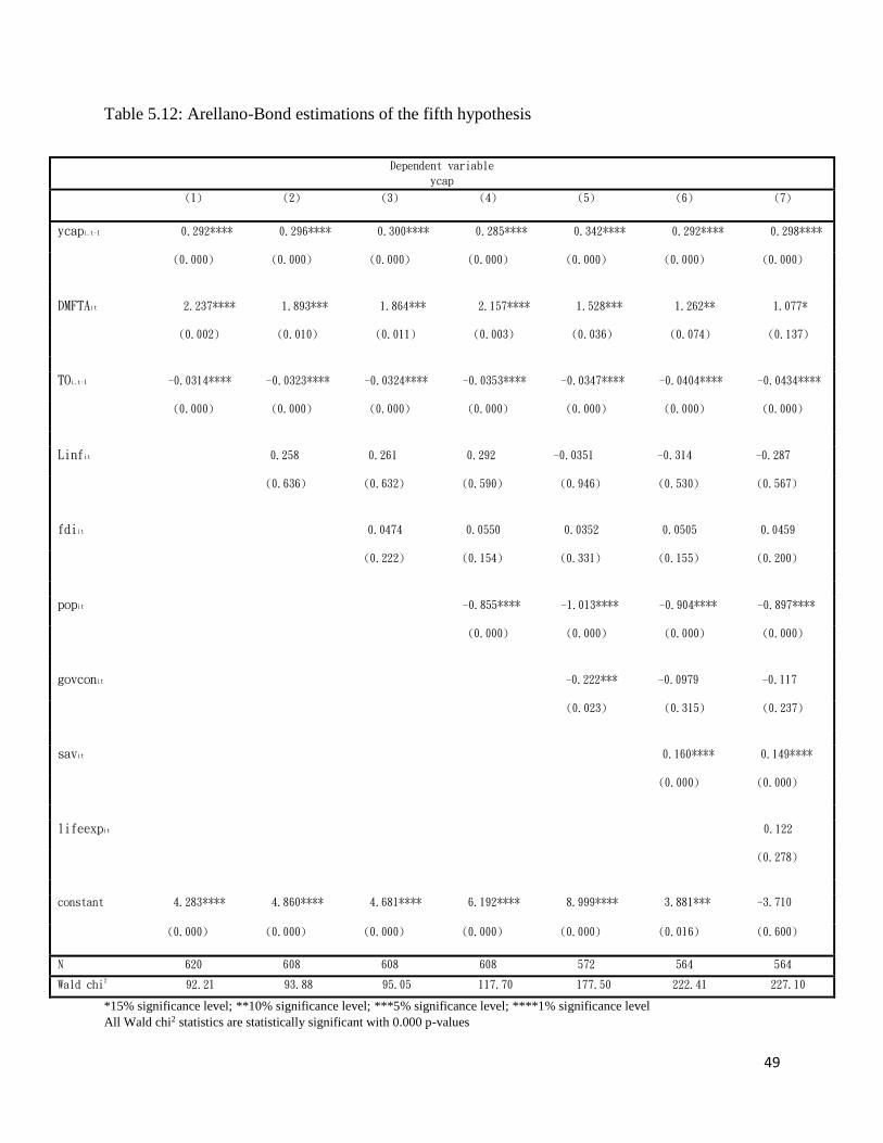
49

Table 5.12: Arellano-Bond estimations of the fifth hypothesis



Dependent variable

ycap

(1) (2) (3) (4) (5) (6) (7)

ycapi,t-1 0.292**** 0.296**** 0.300**** 0.285**** 0.342**** 0.292**** 0.298****

(0.000) (0.000) (0.000) (0.000) (0.000) (0.000) (0.000)

DMFTAit 2.237**** 1.893*** 1.864*** 2.157**** 1.528*** 1.262** 1.077*

(0.002) (0.010) (0.011) (0.003) (0.036) (0.074) (0.137)

TOi,t-1 -0.0314**** -0.0323**** -0.0324**** -0.0353**** -0.0347**** -0.0404**** -0.0434****

(0.000) (0.000) (0.000) (0.000) (0.000) (0.000) (0.000)

Linfit 0.258 0.261 0.292 -0.0351 -0.314 -0.287

(0.636) (0.632) (0.590) (0.946) (0.530) (0.567)

fdiit 0.0474 0.0550 0.0352 0.0505 0.0459

(0.222) (0.154) (0.331) (0.155) (0.200)

popit -0.855**** -1.013**** -0.904**** -0.897****

(0.000) (0.000) (0.000) (0.000)

govconit -0.222*** -0.0979 -0.117

(0.023) (0.315) (0.237)

savit 0.160**** 0.149****

(0.000) (0.000)

lifeexpit 0.122

(0.278)

constant 4.283**** 4.860**** 4.681**** 6.192**** 8.999**** 3.881*** -3.710

(0.000) (0.000) (0.000) (0.000) (0.000) (0.016) (0.600)

N 620 608 608 608 572 564 564

Wald chi2 92.21 93.88 95.05 117.70 177.50 222.41 227.10

50

DMFTAit shows high positive statistical significance at 1% significance level in the dynamic panel

model without the control variables. It remains statistically significant and positive in all of the

equations even with inclusion of savings, unlike bilateral FTAs. The significance level slightly

drops with the introduction of control variables inflation and FDI. With the introduction of popit,

DMFTAit becomes statistically significant at 1% significance level. The coefficient value also

increases in this equation. The significance level drops again with inclusion of govconit. The

significance level again 10% with introduction of savings. In the last equation DMFTAit still

exhibits positive statistical significance. One interesting observation, DMFTAit gradually decreases

in its coefficient value until population growth is introduced. There is a jump in equation 4 and

then it gradually decreases again. This validates the findings of Lehmann and O’Rourke (2008);

Nunn and Trefler (2004). Both of the studies found countries with controlled trade openness

towards higher returns and export oriented domestic sectors experienced higher growth. One

possible explanation of why DMFTAit retains its statistical significance with higher domestic

savings but DBFTAit loses its; is multilateral FTAs are generally conducted between a country and

a trade bloc. MFTAs covers greater trade areas than that of BFTAs. Higher domestic savings may

be sufficient to offset the BFTA effects, it is not enough in magnitude to offset the total trade effect

of MFTAs.

Based on the above estimations it is concluded MFTAs displays positive and significant effect on

economic advancement in presence of trade openness. Hypothesis five is proven true.

5.2.6 Hypothesis 6

The sixth hypothesis examines the negative effect of BFTA on economic progress of LDCs with

dummy variable Bldcit which takes a value of 1 when a LDC has a bilateral FTA and 0 otherwise.

The benchmark OLS regression shows positive and statistically insignificant effect of BFTAs on

economic progression of LDCs in both models. All of the control variables are significant with

expected signs except life expectancy which is insignificant.

51


Dependent variable

ycap

Without control

variables

With control

variables

yinitiali,t0 -0.000124**** -0.000120****

(0.000) (0.001)

Bldcit 0.203 0.146

(0.856) (0.881)

Linfit -3.784****

(0.000)

fdiit 0.0508*

(0.122)

popit -0.861****

(0.000)

govconit -0.278****

(0.000)

savit 0.0475****

(0.003)

lifeexpit -0.0552

(0.303)

constant 4.276**** 7.453***

(0.000) (0.039)

N 727 661

R-sq 0.3348 0.5709


Lagged ycapi,t-1 is highly statistically significant and positive in every Arellano-Bond equations.

The dummy variable Bldcit is negative in the first equation without control variables. It is

statistically insignificant in presence of inflation, fdiit and popit. However, it becomes statistically

significant at 15% significance level with the inclusion of government consumption expenditure.

It becomes highly statistically significant at 5% significance level with inclusion of savit. The

significance level again increases to 15% with introduction of life expectancy. Bldcit exhibits a

negative effect in all three of the statistically significant equations.

All the control variables remains statistically significant since their inclusion of the in the equations

with expected signs. Apart from FDI and lifeexpit which are statistically significant at 5% and 10%

significance level respectively; all the other control variables are statistically significant at 1%

significance level.

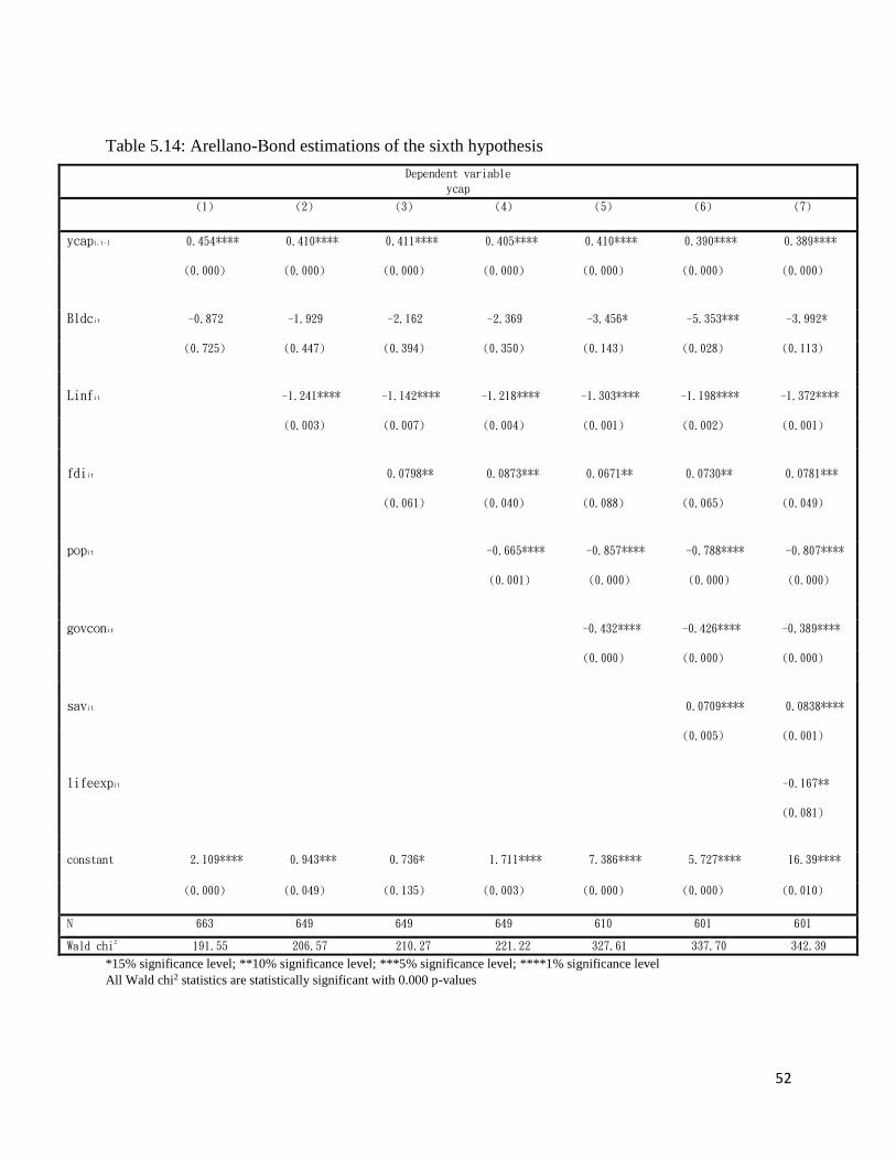
52

Table 5.14: Arellano-Bond estimations of the sixth hypothesis



Dependent variable

ycap

(1) (2) (3) (4) (5) (6) (7)

ycapi,t-1 0.454**** 0.410**** 0.411**** 0.405**** 0.410**** 0.390**** 0.389****

(0.000) (0.000) (0.000) (0.000) (0.000) (0.000) (0.000)

Bldcit -0.872 -1.929 -2.162 -2.369 -3.456* -5.353*** -3.992*

(0.725) (0.447) (0.394) (0.350) (0.143) (0.028) (0.113)

Linfit -1.241**** -1.142**** -1.218**** -1.303**** -1.198**** -1.372****

(0.003) (0.007) (0.004) (0.001) (0.002) (0.001)

fdiit 0.0798** 0.0873*** 0.0671** 0.0730** 0.0781***

(0.061) (0.040) (0.088) (0.065) (0.049)

popit -0.665**** -0.857**** -0.788**** -0.807****

(0.001) (0.000) (0.000) (0.000)

govconit -0.432**** -0.426**** -0.389****

(0.000) (0.000) (0.000)

savit 0.0709**** 0.0838****

(0.005) (0.001)

lifeexpit -0.167**

(0.081)

constant 2.109**** 0.943*** 0.736* 1.711**** 7.386**** 5.727**** 16.39****

(0.000) (0.049) (0.135) (0.003) (0.000) (0.000) (0.010)

N 663 649 649 649 610 601 601

Wald chi2 191.55 206.57 210.27 221.22 327.61 337.70 342.39

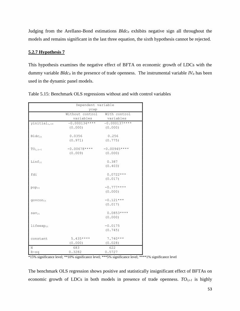
53

Judging from the Arellano-Bond estimations Bldcit exhibits negative sign all throughout the

models and remains significant in the last three equation, the sixth hypothesis cannot be rejected.

5.2.7 Hypothesis 7

This hypothesis examines the negative effect of BFTA on economic growth of LDCs with the

dummy variable Bldcit in the presence of trade openness. The instrumental variable IVit has been

used in the dynamic panel models.


Dependent variable

ycap

Without control

variables

With control

variables

yinitiali,t0 -0.000134**** -0.000137****

(0.000) (0.000)

Bldcit 0.0356 0.256

(0.971) (0.775)

TOi,t-1 -0.00678**** -0.00945****

(0.009) (0.000)

Linfit 0.387

(0.403)

fdi 0.0722***

(0.017)

popit -0.777****

(0.000)

govconit -0.121***

(0.017)

savit 0.0853****

(0.000)

lifeexpit -0.0175

(0.745)

constant 5.435**** 7.740***

(0.000) (0.028)

N 683 622

R-sq 0.3282 0.5727


The benchmark OLS regression shows positive and statistically insignificant effect of BFTAs on

economic growth of LDCs in both models in presence of trade openness. TOi,t-1 is highly

54

statistically significant and negative both with and without control variables. yinitiali,t0 is highly

statistically significant in both models.

Table 5.16: Arellano-Bond estimations of the seven hypothesis



Dependent variable

ycap

(1) (2) (3) (4) (5) (6) (7)

ycapi,t-1 0.272**** 0.279**** 0.283**** 0.267**** 0.328**** 0.278**** 0.290****

(0.000) (0.000) (0.000) (0.000) (0.000) (0.000) (0.000)

Bldcit 2.507 1.653 1.626 1.355 -0.459 -2.800 -3.600**

(0.269) (0.477) (0.485) (0.558) (0.829) (0.179) (0.091)

TOi,t-1 -0.0245**** -0.0266**** -0.0268**** -0.0283**** -0.0297**** -0.0356**** -0.0413****

(0.000) (0.000) (0.000) (0.000) (0.000) (0.000) (0.000)

Linfit 0.241 0.244 0.271 -0.0865 -0.385 -0.324

(0.658) (0.655) (0.618) (0.867) (0.441) (0.517)

fdiit 0.0482 0.0557* 0.0311 0.0489 0.0418

(0.215) (0.150) (0.391) (0.168) (0.241)

popit -0.796**** -1.010**** -0.901**** -0.893****

(0.000) (0.000) (0.000) (0.000)

govconit -0.230*** -0.104 -0.137

(0.019) (0.284) (0.166)

savit 0.172**** 0.153****

(0.000) (0.000)

lifeexpit 0.205**

(0.070)

constant 5.014**** 5.518**** 5.324**** 6.829**** 9.661**** 4.163**** -8.661

(0.000) (0.000) (0.000) (0.000) (0.000) (0.009) (0.227)

N 620 608 608 608 572 564 564

Wald chi2 83.40 87.44 88.76 108.64 172.62 222.13 229.27

55

Lagged ycapi,t-1 is highly statistically significant in each dynamic panel equations. Bldcit is positive

and statistically insignificant in the regression model without control variables. It shows gradual

decrease in its positive value with each additional control variable while remaining statistically

insignificant. The dummy variable changes its sign to negative from positive with the inclusion of

govconit which is statistically significant in the equation. Bldcit remains negative in the rest of the

equation. In the final equation with all the control variable Bldcit becomes statistically significant

at 10% significance level. Trade openness is negative and highly statistically significant in all the

dynamic panel models.

Bldcit shows both positive and negative effect on economic growth in the presence of trade

openness. However, as it is statistically significant in the last equation of the dynamic panel model

the paper cannot completely reject hypothesis seven.

5.2.8 Hypothesis 8

The eight hypothesis examines the negative effect of MFTA on economic growth of LDCs with

the dummy variable Mldcit which takes a value of 1 when a LDC has a multilateral FTA and 0

otherwise. This model tests the effect of multilateral FTAs on LDC’s economic growth

individually without the presence of trade openness.

The benchmark OLS regressions show Mldcit is positive and statistically insignificant in both of

the model. The coefficient value of Mldcit drops noticeably in the presence of the control variables.

The initial level per capita GDP is highly statistically significant in both of the OLS models. In the

second equation in the control variables are statistically significant with proper signs in line with

economic theories except life expectancy. Life expectancy is statistically insignificant and

negative in coefficient value.

56


Dependent variable

ycap

Without control

variables

With control

variables

yinitiali,t0 -0.000118**** -0.000121****

(0.000) (0.001)

Mldcit 0.841 0.249

(0.278) (0.715)

Linfit -3.751****

(0.000)

fdiit 0.0515*

(0.112)

popit -0.866****

(0.000)

govconit -0.260****

(0.000)

savit 0.0482****

(0.002)

lifeexpit -0.0527

(0.310)

constant 4.113**** 7.044***

(0.000) (0.047)

N 727 661

R-sq 0.3370 0.5845


The dyanmic panel model exhibits positive and highly statistically significant values for the lagged

per capita GDP growth. Mldcit is negative and statistically insignificant in individual Arellano-

Bond model. The dummy variable remains statistically insignificant with inclusion of inflation,

fdiit, popit respectivly. With the introduction of govcon it becomes statistically significant at 15%

significance level. The significance level increases to 5% in the inclusion of domestic savings. It

drops to 10% significance level when lifeexp is introduced in the last dynamic panel model. Mldcit

exhibits negative sign in all the dynamic panel models. A similarity can be observed here with that

of hypothesis six is that in both cases the dummy variables become statistically significant when

government consumption expenditur is introducted in the dynamic panel model. govconit is highly

statistically significant and negative in equation 5,6 and 7. Past literature has found higher

government expenditure leads to lower economic growth. Afonso and Furceri (2008) showed 1

percentage point rise in the government spending to GDP ratio decreses growth in the OECD by

0.12% and in the European Union by 0.13%. As LDCs suffer from the basic economic phenomena-

scarcity of resources, higher government expenditure shifts the distribution of resources from

export orinted industries. The negative effect also signifies that the LDCs import more under the

MFTAs compared to their export counterpart.

57

Table 5.18: Arellano-Bond estimations of the eight hypothesis

Dependent variable

ycap

(1) (2) (3) (4) (5) (6) (7)

ycapi,t-1 0.452**** 0.408**** 0.409**** 0.404**** 0.410**** 0.390**** 0.389****

(0.000) (0.000) (0.000) (0.000) (0.000) (0.000) (0.000)

Mldcit -1.646 -1.994 -2.105 -2.320 -2.338* -3.503*** -2.825**

(0.320) (0.248) (0.222) (0.178) (0.139) (0.031) (0.086)

Linfit -1.254**** -1.156**** -1.235**** -1.312**** -1.220**** -1.397****

(0.003) (0.006) (0.004) (0.001) (0.002) (0.001)

fdiit 0.0797** 0.0872*** 0.0668** 0.0722** 0.0778***

(0.061) (0.041) (0.090) (0.068) (0.050)

popit -0.673**** -0.862**** -0.796**** -0.817****

(0.001) (0.000) (0.000) (0.000)

govconit -0.429**** -0.424**** -0.387****

(0.000) (0.000) (0.000)

savit 0.0657**** 0.0807****

(0.008) (0.002)

lifeexpit -0.175**

(0.063)

constant 2.345**** 1.160*** 0.957** 1.969**** 7.542**** 6.061**** 17.16****

(0.000) (0.031) (0.081) (0.002) (0.000) (0.000) (0.006)

N 663 649 649 649 610 601 601

Wald chi2 192.61 207.50 211.18 222.44 327.58 335.82 341.22



Based on the above estimations it is possible to observe that LDCs do experience a negative effect

on economic growth through multilateral FTAs. Therefore, hypothesis eight cannot be rejected.

58

5.2.9 Hypothesis 9

The final hypothesis of the research inspects the negative effect of MFTA on economic growth of

LDCs with dummy variable Mldcit in the presence of trade openness. The instrumental variable

IVit has been used in the dynamic panel models.


Dependent variable

ycap

Without control

variables

With control

variables

yinitiali,t0 -0.000131**** -0.000135****

(0.000) (0.000)

Mldcit 0.438 0.659

(0.540) (0.310)

TOi,t-1 -0.00680**** -0.00938****

(0.008) (0.000)

Linfit 0.409

(0.377)

fdiit 0.0727***

(0.016)

popit -0.776****

(0.000)

govconit -0.113***

(0.027)

savit 0.0854****

(0.000)

lifeexpit -0.0137

(0.795)

constant 5.344**** 7.285***

(0.000) (0.036)

N 683 622

R-sq 0.3202 0.5772


The benchmark OLS regression shows positive and statistically insignificant effect of MFTAs on

growth of LDCs in both models in presence of trade openness. TOi,t-1 is highly statistically

significant and negative both with and without control variables. The coefficient value of trade

openness is small.

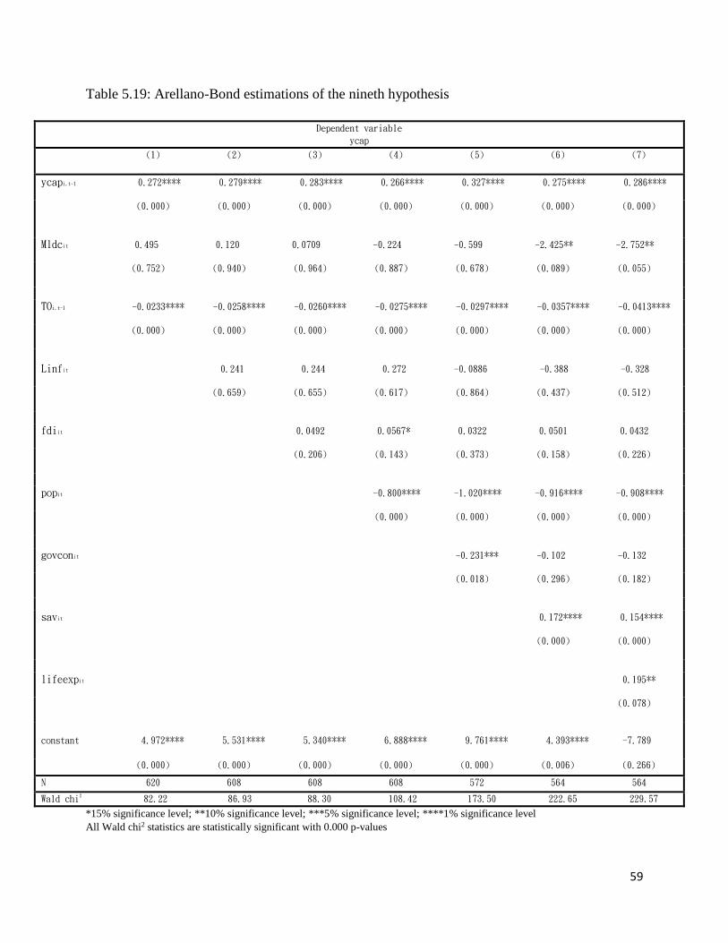
59

Table 5.19: Arellano-Bond estimations of the nineth hypothesis



Dependent variable

ycap

(1) (2) (3) (4) (5) (6) (7)

ycapi,t-1 0.272**** 0.279**** 0.283**** 0.266**** 0.327**** 0.275**** 0.286****

(0.000) (0.000) (0.000) (0.000) (0.000) (0.000) (0.000)

Mldcit 0.495 0.120 0.0709 -0.224 -0.599 -2.425** -2.752**

(0.752) (0.940) (0.964) (0.887) (0.678) (0.089) (0.055)

TOi,t-1 -0.0233**** -0.0258**** -0.0260**** -0.0275**** -0.0297**** -0.0357**** -0.0413****

(0.000) (0.000) (0.000) (0.000) (0.000) (0.000) (0.000)

Linfit 0.241 0.244 0.272 -0.0886 -0.388 -0.328

(0.659) (0.655) (0.617) (0.864) (0.437) (0.512)

fdiit 0.0492 0.0567* 0.0322 0.0501 0.0432

(0.206) (0.143) (0.373) (0.158) (0.226)

popit -0.800**** -1.020**** -0.916**** -0.908****

(0.000) (0.000) (0.000) (0.000)

govconit -0.231*** -0.102 -0.132

(0.018) (0.296) (0.182)

savit 0.172**** 0.154****

(0.000) (0.000)

lifeexpit 0.195**

(0.078)

constant 4.972**** 5.531**** 5.340**** 6.888**** 9.761**** 4.393**** -7.789

(0.000) (0.000) (0.000) (0.000) (0.000) (0.006) (0.266)

N 620 608 608 608 572 564 564

Wald chi2 82.22 86.93 88.30 108.42 173.50 222.65 229.57

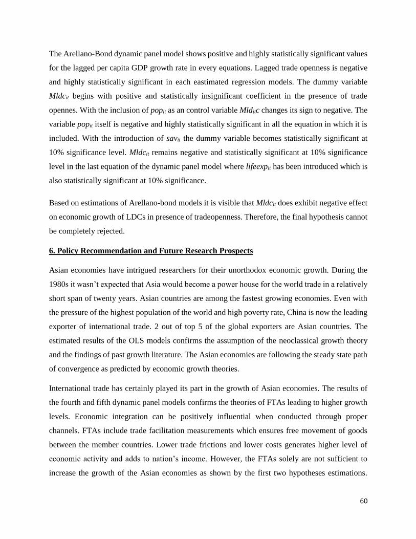
60

The Arellano-Bond dynamic panel model shows positive and highly statistically significant values

for the lagged per capita GDP growth rate in every equations. Lagged trade openness is negative

and highly statistically significant in each eastimated regression models. The dummy variable

Mldcit begins with positive and statistically insignificant coefficient in the presence of trade

opennes. With the inclusion of popit as an control variable Mlditc changes its sign to negative. The

variable popit itself is negative and highly statistically significant in all the equation in which it is

included. With the introduction of savit the dummy variable becomes statistically significant at

10% significance level. Mldcit remains negative and statistically significant at 10% significance

level in the last equation of the dynamic panel model where lifeexpit has been introduced which is

also statistically significant at 10% significance.

Based on estimations of Arellano-bond models it is visible that Mldcit does exhibit negative effect

on economic growth of LDCs in presence of tradeopenness. Therefore, the final hypothesis cannot

be completely rejected.

6. Policy Recommendation and Future Research Prospects

Asian economies have intrigued researchers for their unorthodox economic growth. During the

1980s it wasn’t expected that Asia would become a power house for the world trade in a relatively

short span of twenty years. Asian countries are among the fastest growing economies. Even with

the pressure of the highest population of the world and high poverty rate, China is now the leading

exporter of international trade. 2 out of top 5 of the global exporters are Asian countries. The

estimated results of the OLS models confirms the assumption of the neoclassical growth theory

and the findings of past growth literature. The Asian economies are following the steady state path

of convergence as predicted by economic growth theories.

International trade has certainly played its part in the growth of Asian economies. The results of

the fourth and fifth dynamic panel models confirms the theories of FTAs leading to higher growth

levels. Economic integration can be positively influential when conducted through proper

channels. FTAs include trade facilitation measurements which ensures free movement of goods

between the member countries. Lower trade frictions and lower costs generates higher level of

economic activity and adds to nation’s income. However, the FTAs solely are not sufficient to

increase the growth of the Asian economies as shown by the first two hypotheses estimations.

61

They need to be combined with proper trade openness measurements to enjoy the positive impact

on growth. A recommendation to the policy makers would be to carefully calculate the gains from

exports against the costs of imports not only from the direct FTA partners but also from the

externality generated by the FTAs and only opt for FTAs if the gains outweighs the costs.

Trade openness is negatively effects economic growth as it has been proven by the third hypothesis

and also in the other estimations. Although it may seem unorthodox to experience a negative

impact of trade openness it is not unprecedented as it has been discussed in the literature review.

First explanation of this outcome can be attributed to the measure of trade openness used in this

study. Past literature have used only export growth, import tariff decline and trade volume

separately whereas this study has used an index for trade openness. The index uses trade volume

as a ratio of lagged value of GDP. This approach liberates the index from reverse causality and

contemporaneous effect suffered by the measurements used in past studies. Another explanation

for this phenomena is the Financial Crisis of late 2000s. The world economy suffered prominently

in the Financial Crisis beginning in 2007. This resulted in extensive decrease of the purchasing

power of the western economies which are the major consumers of Asian exports. The crisis also

resulted in dramatic increase of food prices in the world. The majority of the Asian economy

especially the LDCs are net importers of food. While the income from Asian export sector

declined; food grains being an inelastic product, the volume of import did not decrease in

proportion. This resulted in lower net income level for the Asian economies. The western world

and the Asian exports are still recovering from aftermath of the crisis.

The LDC countries reveals the other side of the trade liberalization. Blindly signing FTAs as a

bandwagon effect will lead to lower growth. The developing economies in Asia achieved their

developing status with none or little assistant from FTAs. The recent rapid growth FTAs are

exhibited by the economies which have already overcame the LDC phase and now possess

substantial resources to tackle the issues that come with opening their economies to foreign

competitors. They are now in possession of the technical knowledge and economic means to utilize

their comparative advantage of trade to maintain a positive balance in their trade account. It would

seem timing of the FTA is crucial. FTA being a two directional tool, the gains from it should be

carefully calculated with the costs of conducting an FTA rather than making an untimely decision

just for the sake of it. The proverb “learn to walk before you can run” can be a motto for the Asian

62

LDCs in this context. It is recommended that the LDCs should commence a FTA only if it

facilitates its export oriented industries in which the LDC has a comparative advantage.

The paper followed a dynamic panel approach to tackle the issue of endogeneity by using the

difference of the variables as instrumental variables along with the separate IV for trade openness.

Selecting a proper instrumental variable has always been a challenge for researchers. Future

research can attempt to investigate the trade openness and FTA aspect of growth with different

instrumental variable approach. Taking a different data sample with a longer time period can also

be tested for significant results of the FTAs as FTAs tend to effect growth in the long run (Hur and

Park, (2012)). This can be an exciting prospect for future researchers.

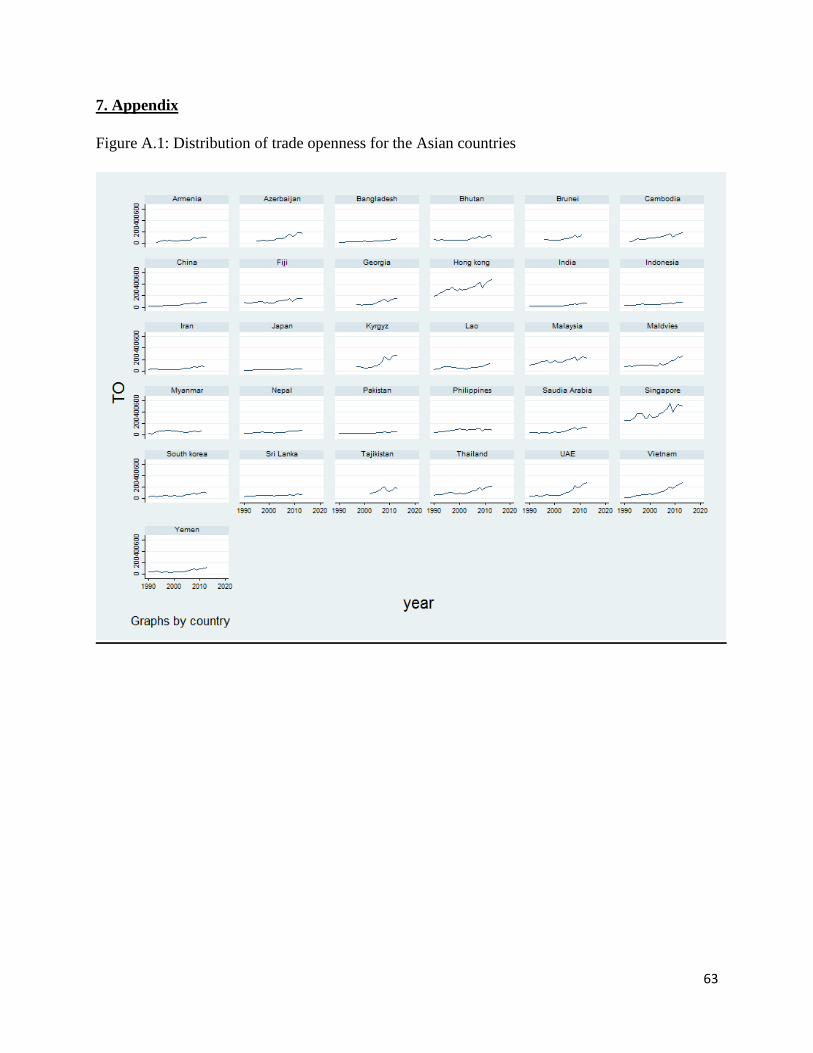
63

7. Appendix

Figure A.1: Distribution of trade openness for the Asian countries

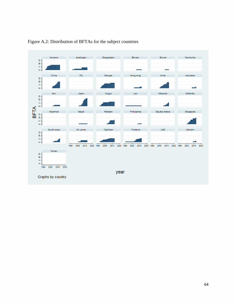
64

Figure A.2: Distribution of BFTAs for the subject countries

65

Figure A.3: Distribution of MFTAs for the subject countries

Table A.1: Statistical summary of original variables

Variable Observations Mean Standard Deviations Minimum Maximum

ycapit 727 3.546468 5.321967 -28.042 32.892

yinitiali,t0 744 5959.228 10948.23 78.40406 45225.2

toit 690 97.81016 89.38046 13.88851 552.8398

infit 725 .6078375 6.445499 -.2209142 154.4438

fdiit 734 3.927131 6.019503 -14.369 50.295

popit 744 1.620441 1.603365 -2.659709 15.0326

govconit 696 12.69264 5.245314 3.46 34.386

savit 687 23.89648 16.66285 -48.712 64.445

lifeexpit 744 69.26361 6.520183 52.462 83.832

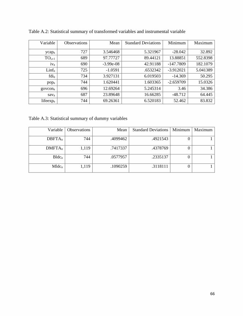
66

Table A.2: Statistical summary of transformed variables and instrumental variable


ycapit 727 3.546468 5.321967 -28.042 32.892

TOi,t-1 689 97.77727 89.44121 13.88851 552.8398

ivit 690 -3.99e-08 42.91188 -147.7809 182.1079

Linfit 725 -1.0591 .6532342 -3.912021 5.041389

fdiit 734 3.927131 6.019503 -14.369 50.295

popit 744 1.620441 1.603365 -2.659709 15.0326

govconit 696 12.69264 5.245314 3.46 34.386

savit 687 23.89648 16.66285 -48.712 64.445

lifeexpit 744 69.26361 6.520183 52.462 83.832

Table A.3: Statistical summary of dummy variables


DBFTAit 744 .4099462 .4921543 0 1

DMFTAit 1,119 .7417337 .4378769 0 1

Bldcit 744 .0577957 .2335137 0 1

Mldcit 1,119 .1090259 .3118111 0 1

67

8. References

Abbas, S., (2014). Trade liberalization and its economic impact on developing and least

developed countries. Journal of International Trade Law and Policy, Vol. 13, No.

3, pp. 215-221

Aitken, Norman D., (1973). The effect of the EEC and EFTA on European trade: a

temporal cross-section analysis. American Economic Review 5, 881–892

(December).

Arellano, M., and Bond, S., (1991). Some tests of specification for panel data: Monte Carlo

evidence and an application to employment equations. Review of Economic Studies

58: 277–297

Baldwin, R. E., (1994). Towards an Integrated Europe. Graduate Institute of International

Studies, Geneva.

Baldwin, R. E., (2003). “Openness and Growth: What’s the Empirical Relationship?”

NBER working paper 9578

Barro, J. R., (1991). Economic Growth in a Cross Section of Countries. The Quarterly

Journal of Economics, Vol. 106, No. 2, pp. 407-443.

Barro, R. and Sala-i-Martin, X., (1995). Economic Growth, New York: McGraw-Hill.

Baier L. S., and Bergstrand H., (2007). Do Free Trade Agreements Actually Increase

Members’ International Trade? Journal of International Economics, 71, 72-95.

Busse, M., and Koeniger, J., (2012) “Trade and Economic Growth: A Re-examination of

the Empirical Evidence”, Institute of International Economics, Hamburg.

Chang, R., Kaltani, L., and Loayza, N. V. (2009). Openness can be good for growth: The

role of policy complementarities. Journal of Development Economics, 90(1), 33–

49.

Chen, M X., and Joshi, S., (2010). Third-country effects on the formation of free trade

agreements. Journal of International Economics 82, 238–248

DeJong, D. N. and M. Ripoll. (2006). Tariffs and growth: An empirical exploration of

contingent relationships. Review of Economics and Statistics 88, (4) (11/01): 625-

40.

Dollar, D., and Kraay, A., (2004). Trade, growth, and poverty. The Economic Journal, 114,

F22−F49.

Ferrarini, A., (2010), “Trade and Income in Asia: Panel Data Evidence from Instrumental

Variable Regression”, ADB Economics Working Paper Series.

68

Folster, S., and Henrekson, M., (2001). Growth Effects of Government Expenditure and

Taxation in Rich Countries. European Economic Review, vol. 45, issue 8, 1501-

1520.

Frankel, J.A., (1997). Regional Trading Blocs. Institute for International Economics,

Washington, DC.

Frankel, J.A., and Romer, D. (1999). “Does trade cause growth?”. American Economic

Review, 89 (3), 379–399.

Ghosh, S. and Yamarik, S., (2004). Are regional trading arrangements trade creating? An

application of extreme bounds analysis. Journal of International Economics 63 (2),

369–395 (July).

Gries, and Redlin, (2012), “Trade Openness and Economic Growth: A Panel Causality

Analysis”, Center for international economics working Paper Series.

Grossman, G., and Helpman E., (1991). Innovation and growth in the global economy.

MIT Press, Cambridge MA and London UK.

Hanushek, E. A., and Woessmann, L., (2012). Do better schools lead to more growth?

Cognitive skills, economic outcomes, and causation. Journal of Economic Growth,

Vol. 17, No. 4, pp. 267-321

Harrison, A., and Rodríguez-Clare, A., (2009). Trade, Foreign Investment, and Industrial

Policy for Developing Countries. NBER Working Paper, No. 15261

Hur, J., and Park, C., (2012). Do Free Trade Agreements Increase Economic Growth of the

Member Countries? World Development Vol. 40, No. 7, pp. 1283–1294

Islam, A., Salim, R., and Bloch, H., (2016). Does Regional Integration Affect Efficiency

and Productivity Growth? Empirical Evidence from South Asia. Review of Urban

and Regional Development Studies Vol. 28, No. 2

Kawai, M., and Wignaraja, G., (2014), Trade Policy and Growth in Asia. ADB Economics

Working Paper Series

Krugman, P. R., (1979). “A Model of Innovation, Technology Transfer, and the World

Distribution of Income,” Journal of Political Economy 87:253–66.

Liu, X., (2016). Trade Agreements and Economic Growth. Southern Economic Journal

Volume 82, Issue 4, Pages 1374–1401

Lehmann Sibulle H. and Kevin H. O’Rourke. (2008). The Structure of Protection and

Growth in the Late 19th Century, NBER Working Paper, No. 14493.

Nunn, N. and D. Trefler, (2004). The Political Economy of Tariffs and Long-term Growth,

revision requested at the American Economic Journal: Macroeconomics.

69

Osang, T., and Pereira, A., (1997). "Savings, Volume of Trade, and Growth," Review of

International Economics, vol. 5(3), pages 310-23,

Rodriguez, F., and Rodrik, D. (2001). Trade policy and economic growth: A skeptic's guide

to the cross-national evidence. In: B. Bernanke, and К. Rogoff (Eds.), NBER

macroeconomics annual 2000. Cambridge, MA: National Bureau of Economic

Research. 2000.

Rodrik, D., (2001). Trading in illusions. Foreign Policy 123, 54– 63 (Mar./Apr.).

Rruka, D. (2004). Decoding the Effects of Trade Volume and Trade Policies on Economic

Growth: A Cross-Country Investigation. http://econwpa.repec.org

Sachs, J. D., and Warner, A. (1995). Economic reform and the process of global

integration. Brookings Papers on Economic Activity, 1, 1-118.

Sohn, C., and Lee, H., (2010). Trade Structure, FTAs, and Economic Growth. Review of

Development Economics, 14(3), 683–698

Stiglitz, J E., (1996). Some Lessons from the East Asian Miracle. World Bank Research

Observer Volume 11, Issue 2, Pp. 151-177.

Tinbergen, J., (1962). Shaping the World Economy. The Twentieth Century Fund, New

York.

Verbeek, M., (2012). “A Guide to Modern Econometics”, John Wiley and Sons Ltd.

Yanikkaya, H. (2003). Trade openness and economic growth: a cross–country empirical

investigation. Journal of Development Economics 72, 57–89.

http://econwpa.repec.org/

Documents

Free Trade Agreements, Trade Openness and Economic Growth