Embed Size (px)
DESCRIPTION
Free trade model
Citation preview

Homepage International Economics
International Economics, Robert A. Mundell, New York: Macmillan, 1968, pp. 3
- 16.
The Classical System
Robert A. Mundell
The distinction, vital to the classical system of international trade theory, between
the short-run mechanism of balance-of-payments adjustment and the static theory
of barter was an important dimension of the classical dichotomy between monetary
theory and value theory. This dichotomy was a powerful tool of analytical
abstraction that enabled a separation of long-run static analysis from short-run
dynamics. In dynamical, short-run, disequilibrium theory, monetary elements
assume a role of first-order importance in the adjustment process. But after the
adjustment process is completed money is shown in its true light as a mere veil,
with no influence upon the nature or position of long-run equilibrium. A major task
of exposition in classical theory, therefore, was to demonstrate the automaticity of
equilibrium through examination of the monetary adjustment process, and through
this demonstration, the unimportance, in the long run, of monetary phenomena.
The demonstration of the automaticity of balance-of-payments adjustment in the
field of international trade theory was a companion to, although it anteceded, the
demonstration of a different kind of automaticity in value theory. In the theory of a
closed economy the classical economists assumed the system tended automatically
toward a full-employment equilibrium, on the premise that money wages were
flexible, and it was an equilibrium not affected, in any fundamental way, by the

amount of money in the system. Whatever the temporary effects of a change in
central bank policy, the money supply had no influence upon the equilibrium rate
of interest, which was identified with the rate of profit, or the real wage. Instead,
money exerted its influence merely upon the price level and the level of money
wages. Since money could not alter either the level of real wages or the rate of
interest, it could not affect the equilibrium level of any real magnitude in the
economic system, and the path was cleared for long-run analysis and abstraction
from purely monetary phenomena.
In an open economy linked to the rest of the world by international trade and the
gold standard, on the other hand, the central bank could not even affect the
nominal quantity of money in the system unless the country was large enough to
influence, by itself, the world price level. Whereas in a closed economy the central
bank could determine the nominal quantity of money, and the public, through
spending or hoarding it, could determine its real value, in an open economy any
excess of new money creation over desired hoarding would escape down the
foreign drain. An overissue of money by the banking system would quickly bring
its own corrective: Specie would flow out and force the banks to take back the
redundant currency, or else suffer a depreciation of the gold value of bank notes.
The nominal quantity of money was thus determined in a single economy by
international considerations, and the barter terms of trade could not be affected
permanently by purely monetary disturbances.
To have perceived the validity of these propositions, which even today exhibit a
fundamental truth, was the supreme intellectual achievement of classical economic
analysis. Through this theory mercantilist fallacies could be refuted and the way
paved for the emphasis on the doctrine of free trade and on other real phenomena,
the only considerations that were supposed to matter in the long run. Ricardo's love

was not the short-run dynamic mechanism but the long-run static theory of
international barter.
We know today that this separation of statical, barter theory from dynamical,
monetary theory was carried too far, in the sense that it cannot be maintained, as
the classical school seemed to hold it could, that the trade equilibrium established
under conditions in which money is used and the trade equilibrium reached under
conditions of barter are identical. Indeed, it is difficult to conceive of a way in
which the assertion can be given an operational meaning. What is valid in the
separation is not the identical nature of the equilibrium that is achieved, but rather
the universality of the principles established in the process of reaching trade
equilibrium. The principles established would not be different and it is this that
provides the justification for an extended treatment of the classical barter model.
The barter model is indeed the source of many propositions that form the body of
modern international trade theory. Despite severe criticism of other aspects of
classical theory the barter model has stood the test of time. Its survival can be
attributed partly to its applicability to current policy issues in the country in which
it originated, and partly to its internal consistency. It was logically immune to
criticisms of general equilibrium and macroeconomic methods and was
aggregative in scope.
The classical school was interested in establishing the direction in which the terms
of trade would move as a result of exogenous disturbances to equilibrium such as
would arise from tariffs, hoarding, harvest failures, income transfers (or other
remittances) and productivity changes. More powerful methods today make it
possible to derive additional implications from the model and to deduce, in cases
where the relevant data are available, the probable magnitude of changes in the

terms of trade. The purpose of this and the following two chapters 1 is to show how
these results may most simply be obtained. The main focus of our attention will be
on comparative statics rather than dynamics or monetary considerations.
Analytical Procedure
The nature of comparative statics analysis is a contrast between two positions,
usually positions of equilibrium, distinguished from one another by a shift in some
parameter such as that which would be brought about by a change in economic
policy. The policy change disturbs the initial equilibrium by causing excess
demand for one commodity and excess supply of another commodity. The
disequilibrium must then be eliminated, if a new equilibrium is to be reached, by
an adjustment in some other variable. The adjusting or equilibrating variable may
be another policy change, or a process of adjustment that is sufficiently predictable
to be considered automatic.
In classical international trade theory the adjustment mechanism was presumed to
be automatic. A policy change would disturb balance-of-payments equilibrium,
induce a gold flow and, through a change in relative price levels, a change in the
terms of trade. Today this mechanism is not so automatic in the sense that central
bank and government reaction to disequilibrium in the balance of payments is
predictable. Besides the traditional inflation-deflation method of the gold standard,
a disequilibrium may be corrected by borrowing (in the short run), trade controls,
tax changes, technological changes (in the long run), or the exchange-rate
adjustment. Most of these methods have been used2 by one country or another
since the breakdown of the gold standard system to resolve balance-of-payments
crises.

Because of this change in institutional response to disequilibrium, any analysis of
policy change necessarily involves elements of taxonomy. Such questions as: "Do
tariffs improve the balance of trade?" cannot be given an equivocal reply; the
answer depends on the other policies followed by the government. A tariff disturbs
the initial equilibrium and therefore requires, for a new equilibrium to be reached,
a change in some other policy; it may involve changes in any or all of the policies
listed above.
But exploring all conceivable policy alternatives would be tedious and
unrewarding pedantry. For that reason it is convenient to assume that, for
analytical purposes, the classical mechanism is operative, that the terms of trade
"automatically" adjust to correct disequilibrium. The first step in the comparative-
static analysis is therefore to determine the effect of policy changes on the terms of
trade or domestic price ratios. It will be shown later that results thus obtained can
be used to demonstrate the working of any alternative mechanisms of adjustment.
The Method of Comparative Statics
The most direct way to derive the effect of a policy change on the terms of trade is
to differentiate a balance-of-payments equation with respect to the change in
policy, and to substitute in the result the conditions necessary to satisfy the other
conditions of equilibrium. A more intuitive way of getting the criterion, however,
is to employ a device implicit in all comparative-statics analysis. This is to
compute the excess demand caused by the policy change on the assumption that
the adjusting variable is constant, and to equate this excess demand to the excess
supply created by the actual change in the adjusting variable. If, for example, we
wish to find the criterion for the effects of a tax on the terms of trade, we first
determine the excess demand caused by the tax at constant terms of trade and
translate the excess demand, which is the coefficient of the tax change, into the
appropriate income or price elasticity; we then compute the excess supply of the
same good created by a change in the terms of trade, translating its coefficient into
the relevant elasticities. By equating the excess demand and the excess supply the
criterion is established.
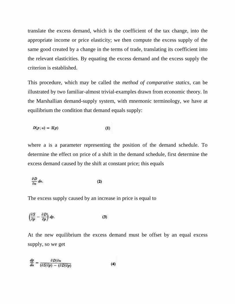
This procedure, which may be called the method of comparative statics, can be
illustrated by two familiar-almost trivial-examples drawn from economic theory. In
the Marshallian demand-supply system, with mnemonic terminology, we have at
equilibrium the condition that demand equals supply:
where a is a parameter representing the position of the demand schedule. To
determine the effect on price of a shift in the demand schedule, first determine the
excess demand caused by the shift at constant price; this equals
The excess supply caused by an increase in price is equal to
At the new equilibrium the excess demand must be offset by an equal excess
supply, so we get

which is the criterion we set out to find.
In the naive Keynesian system we have, at equilibrium, equality of saving (S) and
investment (I), that is,
where y is income and (x is a parameter representing the level of autonomous
investment. To find the effects of a shift in the investment schedule on income,
first consider the excess demand for goods at constant income, that is,
and then the excess supply induced by a change in income, that is,
where s' is the marginal propensity to save. At the new equilibrium the excess
demand caused by the shift in investment and the excess supply created by the
change in income must be equal. Equating (6) and (7) and rearranging terms, we
get the familiar multiplier
A second step in analysis is to utilize information from knowledge of stability. Any
adjustment mechanism implies a type of dynamic behavior and thus a condition of
dynamic stability-convergence to equilibrium over time. If an equilibrium is
unstable, the system would not tend to approach the new equilibrium given by the
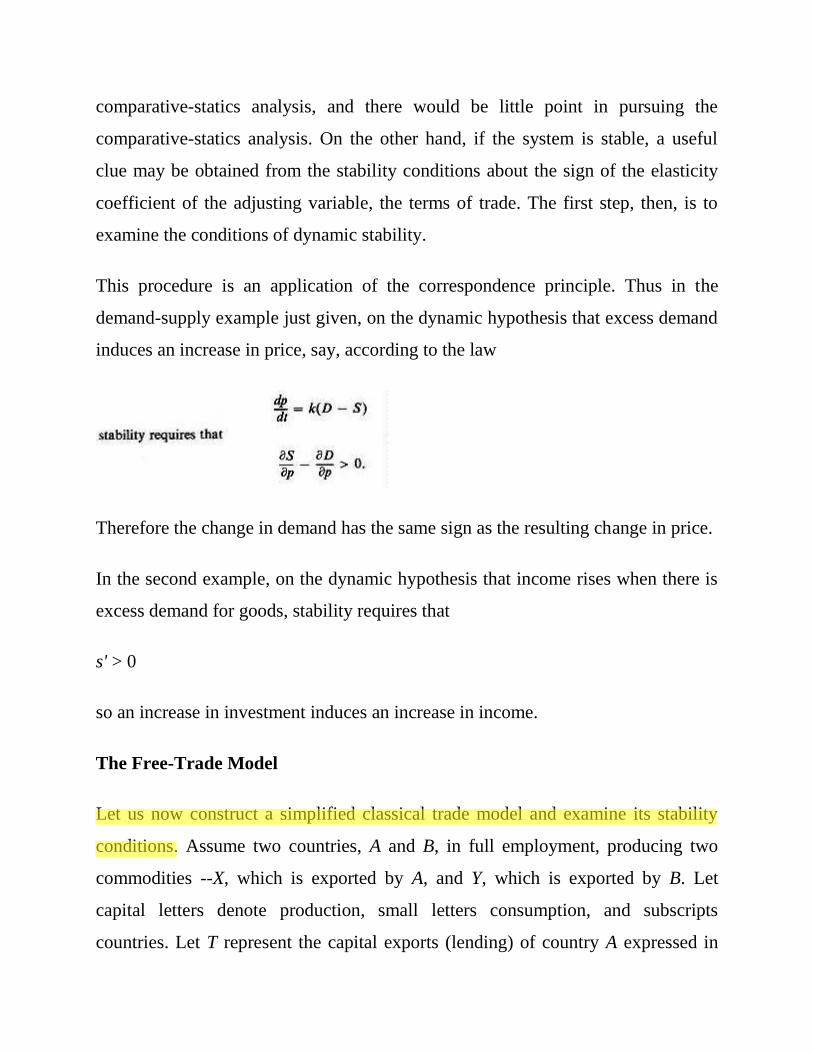
comparative-statics analysis, and there would be little point in pursuing the
comparative-statics analysis. On the other hand, if the system is stable, a useful
clue may be obtained from the stability conditions about the sign of the elasticity
coefficient of the adjusting variable, the terms of trade. The first step, then, is to
examine the conditions of dynamic stability.
This procedure is an application of the correspondence principle. Thus in the
demand-supply example just given, on the dynamic hypothesis that excess demand
induces an increase in price, say, according to the law
Therefore the change in demand has the same sign as the resulting change in price.
In the second example, on the dynamic hypothesis that income rises when there is
excess demand for goods, stability requires that
s' > 0
so an increase in investment induces an increase in income.
The Free-Trade Model
Let us now construct a simplified classical trade model and examine its stability
conditions. Assume two countries, A and B, in full employment, producing two
commodities --X, which is exported by A, and Y, which is exported by B. Let
capital letters denote production, small letters consumption, and subscripts
countries. Let T represent the capital exports (lending) of country A expressed in

terms of X; let P denote the terms of trade, the price of Y in terms of X; and let D
represent domestic expenditure.
The system can then be described by the following equations:
Domestic expenditure in A (in terms of X) equals national income minus net capital
exports:
Domestic expenditure in B (in terms of Y) equals national income plus net capital
imports:
The demand for Y in A depends on domestic expenditure and the terms of trade:
The demand for X in B depends on domestic expenditure and the terms of trade:

Figure 1-1.
The dimensions of the box represent world output of the two goods. The
endowment point shows how production is distributed between the two countries
before trade or transfers. The point Q Illustrates post-trade equilibrium on that
assumption that country A makes a transfer to country B and that there is free trade
It is left for the reader to translate the symbols used in the text into distances in the
diagram, to develop an alternative statement of the equilibrium conditions using
community indifference curves and the contract locus, and to show that, in the
variable production case, A's and B's production possibility curves, referred to

origins OA and OB respectively, would be tangent to one another at the pre-transfer
point.
In subsequent diagrams the endowment point will be regarded as the origin for
trade.
The production of X and Y in A depends on the terms of trade:
The production of X and Y in B depends on the terms of trade:
The net capital exports of country A equal the balance of trade of country A:
Variations in domestic expenditure in each country are assumed to depend on
changes in policy. In the free-trade case the system is completed by the following
equations:
We then have eleven independent equations in the twelve unknowns xa, xb, ya, yb,
Xa, Xb, Ya, Yb, Da, Db, P, and T, so there is 1 degree of freedom. Knowing the rate at
which A is lending to B (that is, T), we can solve for the equilibrium terms of trade
(P); or, assuming that the terms of trade are fixed, we can find the rate of lending
that will establish equilibrium.
There are other, equivalent ways of writing the equilibrium conditions of the
system. Equations (9) and (10) could be replaced by conditions stating that world
production and world consumption of each good must be equal -- these alternatives
imply each other when combined with equation (15), expressing balance-of-
payments equilibrium. Equations (11) and (12), the demand functions for the good
that is imported in each country, could be replaced by the demand functions for the
good that is exported, since all income is spent; the part of domestic expenditure
that is not spent on one good must be spent on the other good.
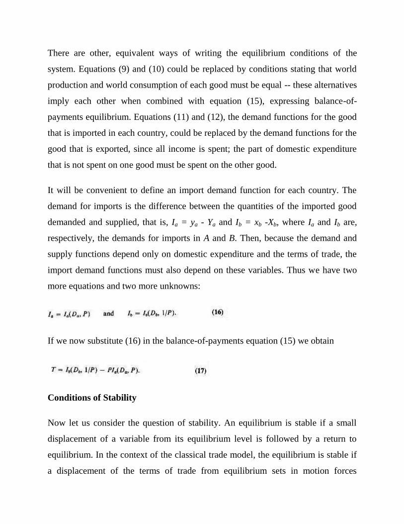
It will be convenient to define an import demand function for each country. The
demand for imports is the difference between the quantities of the imported good
demanded and supplied, that is, Ia = ya - Ya and Ib = xb -Xb, where Ia and Ib are,
respectively, the demands for imports in A and B. Then, because the demand and
supply functions depend only on domestic expenditure and the terms of trade, the
import demand functions must also depend on these variables. Thus we have two
more equations and two more unknowns:
If we now substitute (16) in the balance-of-payments equation (15) we obtain
Conditions of Stability
Now let us consider the question of stability. An equilibrium is stable if a small
displacement of a variable from its equilibrium level is followed by a return to
equilibrium. In the context of the classical trade model, the equilibrium is stable if
a displacement of the terms of trade from equilibrium sets in motion forces

inducing a return to that equilibrium. The system is stable only if a fall in the price
level or exchange rate of the deficit country causes an improvement in its balance
of payments. To find the criterion for stability we have to compute the excess
supply caused by a change in the terms of trade. This criterion will then give us the
coefficient of a change in the terms of trade for use in the comparative-statics
analysis.
The balance of trade surplus of country A, expressed in terms of home goods, can
be written, given the level of domestic expenditure in each country, as
The terms in parentheses are the elasticities of demand for imports in A and B
respectively. Write these terms, with a change of sign, as etaa and etab. Then we
have
If trade is initially in balance, Ib = PIa, so that a fall in A's terms of trade (an
increase in P) will improve or worsen A's trade balance, depending on whether

where I = Ia = Ib, on the assumption of initially balanced trade and choice of
commodity units to make P initially equal to 1. Stability requires that a fall in A's
terms of trade improve A's trade balance, so the system is stable or not
Figure 1-2.
The offer curves OA and OB intersect an initial equilibrium Q. A change in the
terms of trade in the proportion TQ/QM in favor of A creates an excess demand for
B's good and a deficit in A's balance of payments equal to RW (in terms of Y).
Deflationary pressures in A and inflationary pressures in B will therefore reverse
the terms of trade change restoring equilibrium. The system is therefore stable.
The stability conditions are derived as follows: Define the elasticities of demand
for imports in each country.

depending on whether the sum of the elasticities of demand for imports is greater
or less than 1.
This criterion can be derived directly from the dynamic behavior of the system
along the lines that Samuelson, writing in the early 1940s, made famous.
Let us approximate the dynamic behavior of the system by the following
differential equation:
which states that the speed of the change in the terms of trade is proportional to the
discrepancy between foreign exchange payments and receipts. Expanding this
equation in a Taylor series in the neighborhood of equilibrium, omitting nonlinear
terms, and choosing time units to make the "speed of adjustment" k = 1, we obtain
where P0 denotes the terms of trade at equilibrium. This equation has a solution

The equilibrium point is stable only if ; this can be the case only if
the exponential term disappears, that is, only if etaa + etab -1 > 0.3
This discussion has been restricted to the stability of an equilibrium rather than to
the stability of a system. John Stuart Mill recognized the possibility of multiple
equilibria without reference to stability ([66], pp. 15-63), but his treatment was in
error in certain respects. Marshall, in 1879, was aware ([52], pp. 24-25) that a point
of unstable equilibrium must be flanked by points of stable equilibria, that the
number of equilibria must be odd, and that (therefore) if an equilibrium were
unique it would be stable.
There are alternative ways of expressing the stability condition. For example, it can
be expressed in terms of one good only. To see this. recall equation (1), which
expresses the equality of income (plus borrowing) and expenditure in country A.
With lending zero this equation can be written
That is, offers of exports equal the value of imports demanded. Substituting in (18)
and making a similar substitution for Ib, we can write the balance of payments
(with no lending) as

where X is world production and consumption at equilibrium, and the arguments in
the bracket are, respectively, the world elasticity of demand for X and the world
elasticity of supply of X:
where units are chosen so that P is, at equilibrium, equal to unity. By similar
reasoning from the balance-of-payments equation,
we find that
where etay and epsilony are the elasticities of world demand for, and supply of, Y.4
The elasticities of demand for X and Y are defined to be positive provided these
goods are not Giffen goods; and the elasticities of supply of X and Y are defined to
be positive provided opportunity costs are not decreasing. It may then be seen that
the system is necessarily stable if neither good is a Giffen good in world
consumption and opportunity costs are not decreasing. But even if the goods are
Giffen goods, positive supply elasticities may yet make the system stable.
The task of Chapter 2 is to introduce into the balance-of-payments equation
various parameters representing economic policies, and to show how the

equilibrium values of the variables are affected by changes in these policies.
Unless it is explicitly stated to the contrary, the equilibrium point will be assumed
to be stable.5
Price and Income Effects
Before going on to a consideration of changes in economic policies, it will be
useful to introduce a relationship between income propensities and price
elasticities based on Slutsky's separation of price effects into income and
substitution effects. A price elasticity of demand can always be written as the sum
of a compensated (pure substitution) price elasticity and an income propensity.
Consider any demand function of the form I = I(D, P) and differentiate with
respect to P. This yields
after multiplying by P/I. Now -(P/I) deltaI / deltaP is the (money-income constant)
elasticity of demand, eta, and P deltaI / deltaD is the marginal propensity to
spend, m. Thus
A change in price can be associated with a change in real income approximately
equal to the change in cost of the initial amount bought, IdP. If expenditure is
adjusted to compensate for this change in real income, that is, if dD = IdP, then -
(P/I)(dI/dP) becomes the compensated elasticity of demand, eta', and we get
eta = m + n' .6 If indifference curves are convex, all

Figure 1-3
Initial equilibrium is at Q on A's offer curve OA. Suppose that the terms of trade
change in the proportion TQ/QM, and that at the new terms of trade A trades at the
point Q'. The effect on income of this change in the terms of trade can be
approximated by OD in terms of X or TQ in terms of Y, where DQ is drawn
parallel to OT.
To prove the relation between compensated and ordinary elasticities: Define the
elasticity of demand for imports in A, by

which is the elasticity of demand for imports with the income effect removed, i.e.,
the compensated elasticity of demand for imports, eta'a .
substitution effects in the two-good case under consideration are positive, so eta >
0. From this it follows that the elasticity of demand for imports is always greater
than the marginal propensity to import. A fortiori the sum of the elasticities of
demand for imports is greater than the sum of the marginal propensities to import,
so that if ma + mb is equal to, or exceeds, 1, the exchange market is necessarily
stable. Conversely, an unstable exchange market implies that the sum of the
marginal propensities to import is less than unity.
l Adapted from: Amer. Econ. Rev., 50, 68-110 (March, 1960).
2 Often, perhaps usually, to the detriment of economic efficiency. We are
concerned now, however, with "positive," rather than "normative," aspects of
international trade theory.
3 The elasticity criterion just derived was first developed by Alfred Marshall. It is
important, however, to notice that Marshall's dynamic postulates differ from that
described in (20) above. The latter assumes that the budget equations in each
country are satisfied (each country is always at a point on its offer curve) but that
markets are not necessarily cleared. Marshall's postulates are based on adjustments
of offers toward the budget equations (offer curves). Marshall's adjustment
process, which can be justified on the basis of varying profitability of export
industries, admits richer solutions, including the possibility of complex roots and
an oscillatory path to equilibrium (see Samuelson [90], pp. 266-268).

4 Mosak ([68], chap. 4) derived stability conditions in terms of one good only; see
also Johnson ([30], p. 98). See Hirschman [25] for a development of the stability
criterion when trade is not initially in balance.
5 With respect to instability Marshall ([51], p. 354) wrote: ". . . it is not
inconceivable but it is absolutely impossible," a statement I find understandable if
not comprehensible ! More complicated aspects of stability in the classical system
are explored in Chapters 3 and 7.
6 Meade [54] has made extensive use of this relation, his stability condition is split
into income and substitution effects and, in my notation. is eta'a + eta'b + ma + mb -
1 > 0.
Literature Cited
[25] A. O. HIRSCHMAN, "Devaluation and the Trade Balance: A Note," Rev.
Econ. Stat., 31, 50-53 (Feb.1949).
[30] H . G . JOHNSON, " Economic Expansion and International Trade,"
Manchester School Econ. Soc. Stud., 23, 95-112 (May 1955).
[51] A. MARSHALL, Money Credit and Commerce. London: Macmillan, 1923.
[54] J. E. MEADE, "A Geometrical Representation of Balance-of-Payments
Policy," Economica, 16, 305-320 (Nov. 1949).
[68] J. L. MOSAK, General Equilibrium Theory in International Trade.
Bloomington: Indiana University Press, 1944.

[90] P. A. SAMUELSON, " The Transfer Problem and Transport Costs: I, The
Terms of Trade When Impediments Are Absent, II, Analysis of Effects of Trade
Impediments," Econ. Jour., 57, 278-304 (June 1952); 59, 264 290 (June 1954).
© Copyright Robert A. Mundell, 1968