Frequency doubling in aviscoelastic mixing layer

François Sausset, Olivier Cadot & Satish Kumar

Laboratoire PMMH, ESPCI, France.

Laboratoire UME, ENSTA, France.

University of Minnesota, USA.

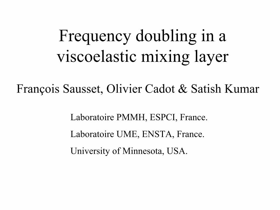
The mixing layer

(*)

• Basically a Kelvin Helmholtz type instability

• Non linear effect as vortex formation and merging, subharmonics production

*Ho & Huang (1982)

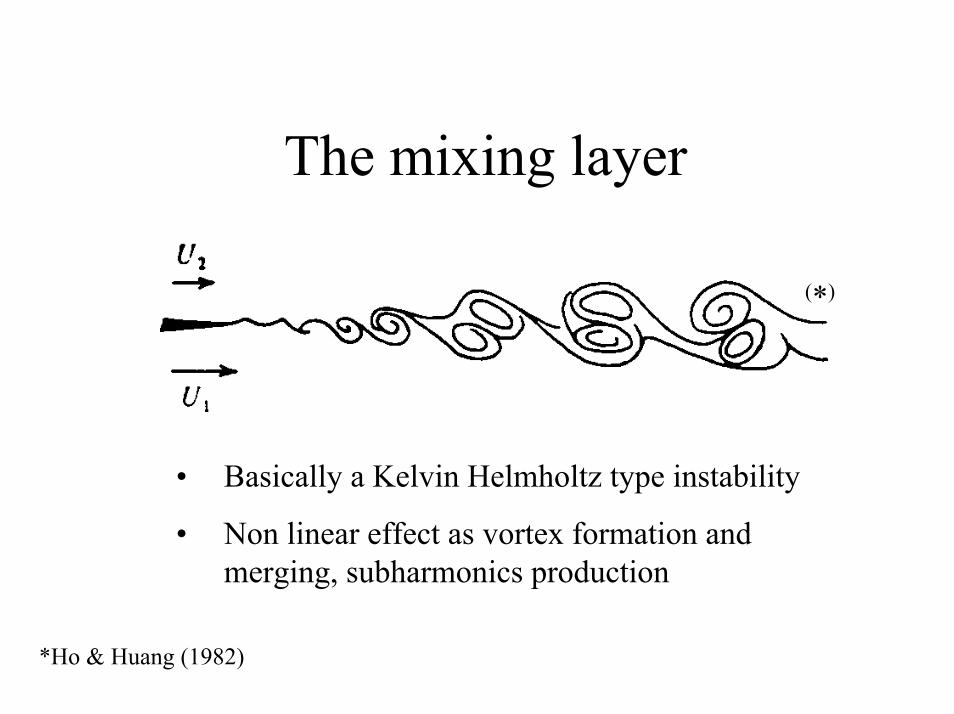
Viscoelastic mixing layerLow Re• Linear stability analysis of Azaiez & Homsy (1994): Elasticity stabilizes

similarly to that of surface tension in Newtonian K-H instability : λ ↑, σ ↓.• 2D and 3D Numerical simulations : stabilization mechanism of Azaiez &

Homsy only slightly pronounced in Yu & Phan-Thien (2004) or Lin & Fan (1999).Kumar & Homsy (1999) found a different stabilization due to the suppression of the fundamental of the instability but leading to a strong harmonic :

Newtonian Elastic

Viscoelastic mixing layer

High Re• Experiments of Hibberd Kwad & Scharf (1982) or Riedigers (1989) show a

suppression of small scales structures and longer lifetime of large structures.

⇒ Experiment at Low Re comparable to the numerical simulation of Kumar & Homsy (1999)

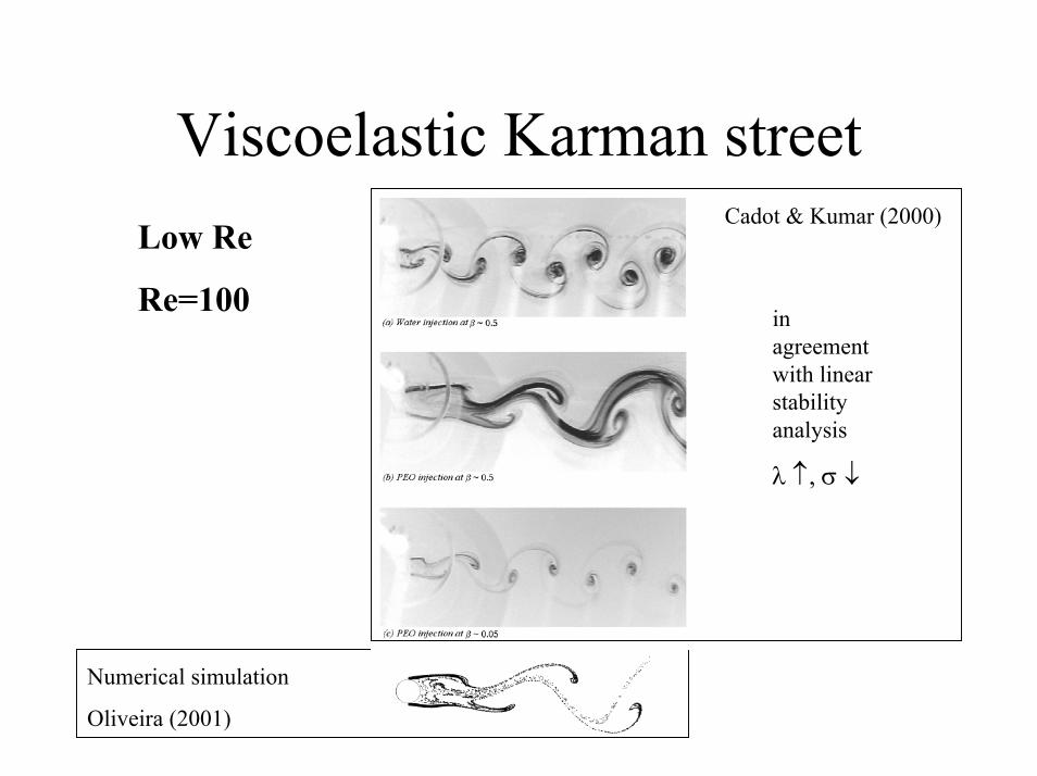
Viscoelastic Karman street

Numerical simulation

Oliveira (2001)

Low Re

Re=100 in agreement with linear stability analysis

λ ↑, σ ↓

Cadot & Kumar (2000)

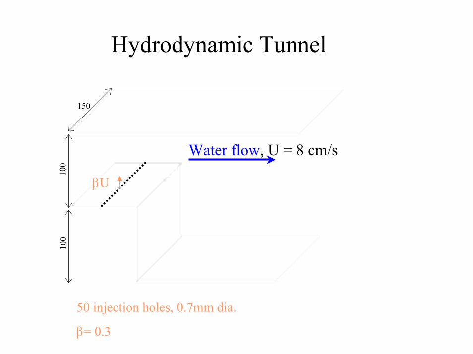
Hydrodynamic Tunnel10

010

0

150

βU

50 injection holes, 0.7mm dia.

β= 0.3

Water flow, U = 8 cm/s

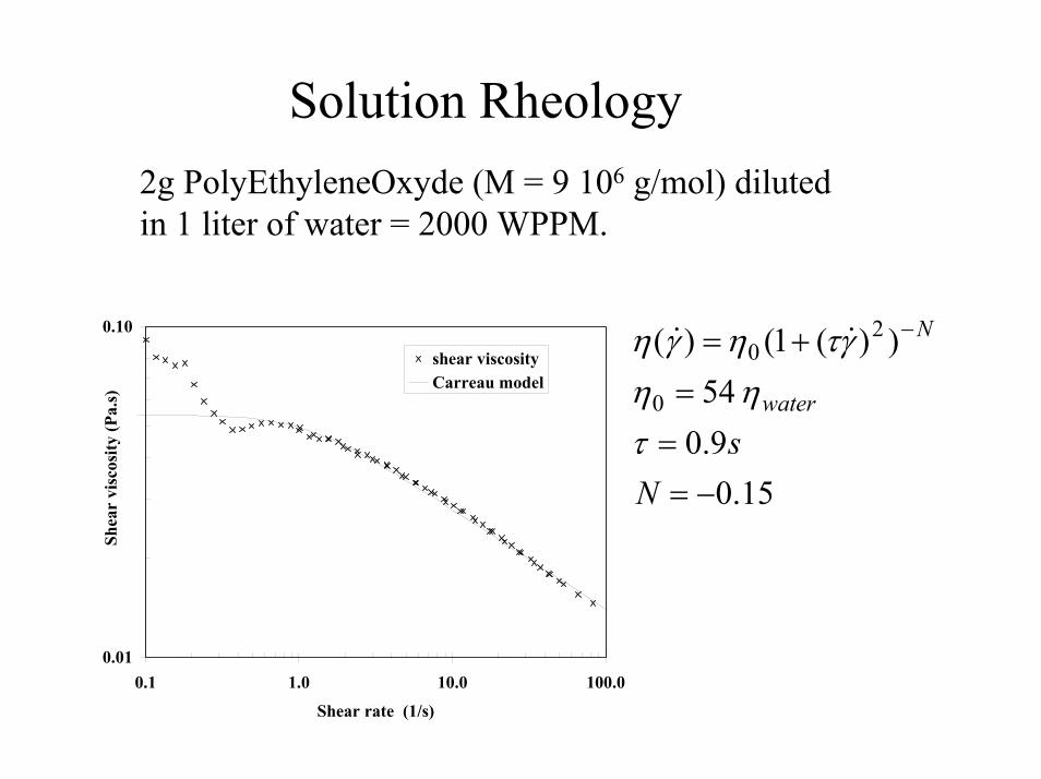
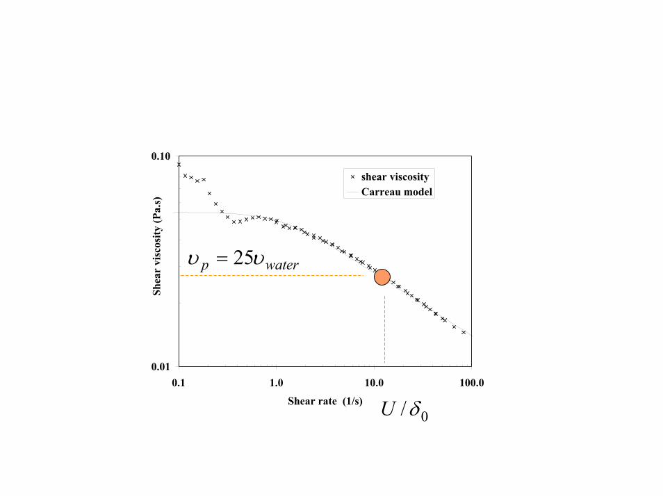
Solution Rheology2g PolyEthyleneOxyde (M = 9 106 g/mol) diluted in 1 liter of water = 2000 WPPM.

0.01

0.10

0.1 1.0 10.0 100.0Shear rate (1/s)

Shea

r vi

scos

ity (P

a.s)

shear viscosityCarreau model

15.09.054

))(1()(

0

20

−===

+= −

Ns

water

N

τηη

γτηγη &&

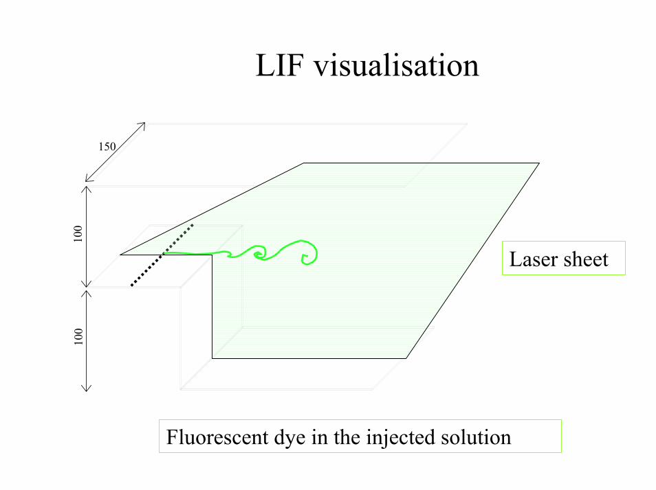
LIF visualisation10

010

0

150

Fluorescent dye in the injected solution

Laser sheet

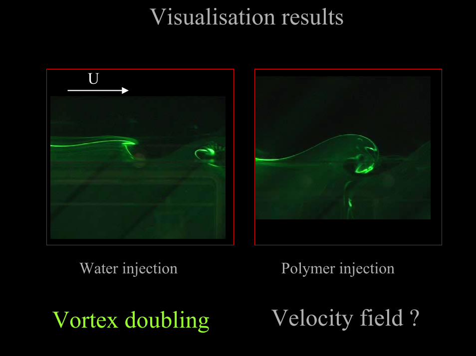
Visualisation results

U

Water injection Polymer injection

Velocity field ?Vortex doubling

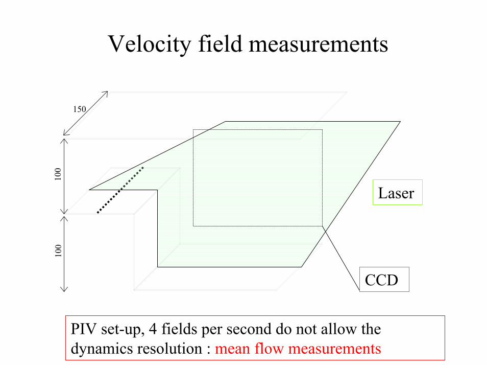
Velocity field measurements10

010

0

150

Laser

CCD

PIV set-up, 4 fields per second do not allow the dynamics resolution : mean flow measurements

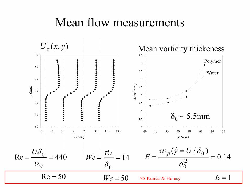
Mean flow measurements

-50

-30

-10

10

30

50

70

-10 10 30 50 70 90 110 130

x (mm)

y (m

m)

),( yxU x

∫∫

=

>=<

dydy

yxdU

dydy

yxdUyx

dyyxdUyx

x

x

x

),(

),(

)(

),(),(

2

2δ

ω

Mean vorticity thickeness

4

4.5

5

5.5

6

6.5

7

7.5

8

8.5

-10 10 30 50 70 90 110 130

x (mm)de

lta (m

m)

Polymer

Water

δ0 ~ 5.5mm

440Re 0 ==w

Uυδ

140

==δτUWe 14.0

)/(20

0 ==

=δ

δγτυ UE p &

50Re = 50=We 1=ENS Kumar & Homsy

0.01

0.10

0.1 1.0 10.0 100.0Shear rate (1/s)

Shea

r vi

scos

ity (P

a.s)

shear viscosityCarreau model

waterp υυ 25=

0/δU

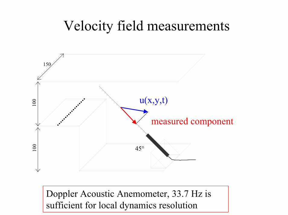
Velocity field measurements10

010

0

150

45°

u(x,y,t)

measured component

Doppler Acoustic Anemometer, 33.7 Hz is sufficient for local dynamics resolution

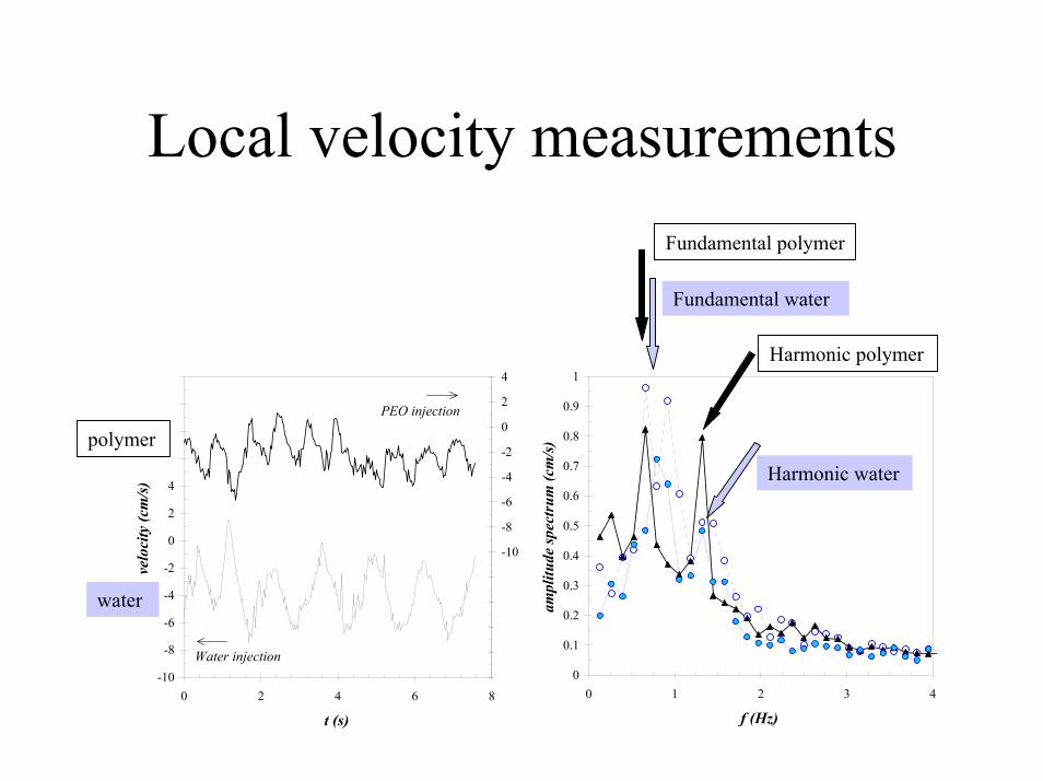
Local velocity measurements

⇒ Frequency doubling

Spectrum analysis

0

0.1

0.2

0.3

0.4

0.5

0.6

0.7

0.8

0.9

1

0 1 2 3 4

f (Hz)

ampl

itude

spec

trum

(cm

/s)

Fundamental water

Harmonic water

Fundamental polymer

Harmonic polymer

-10

-8

-6

-4

-2

0

2

4

6

8

10

12

0 2 4 6 8

t (s)

velo

city

(cm

/s)

-20

-18

-16

-14

-12

-10

-8

-6

-4

-2

0

2

4

Water injection

PEO injection

water

polymer

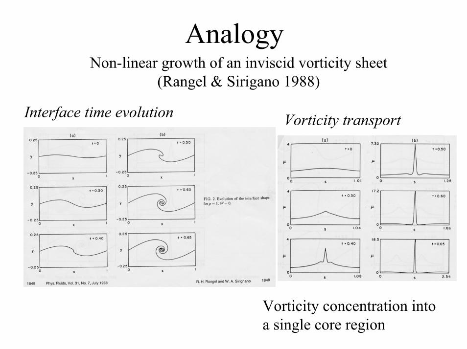
AnalogyNon-linear growth of an inviscid vorticity sheet

(Rangel & Sirigano 1988)

Interface time evolution Vorticity transport

Vorticity concentration into a single core region

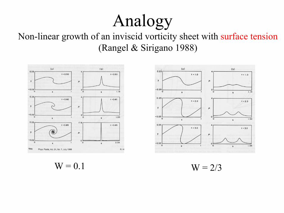
AnalogyNon-linear growth of an inviscid vorticity sheet with surface tension

(Rangel & Sirigano 1988)

W = 0.1 W = 2/3

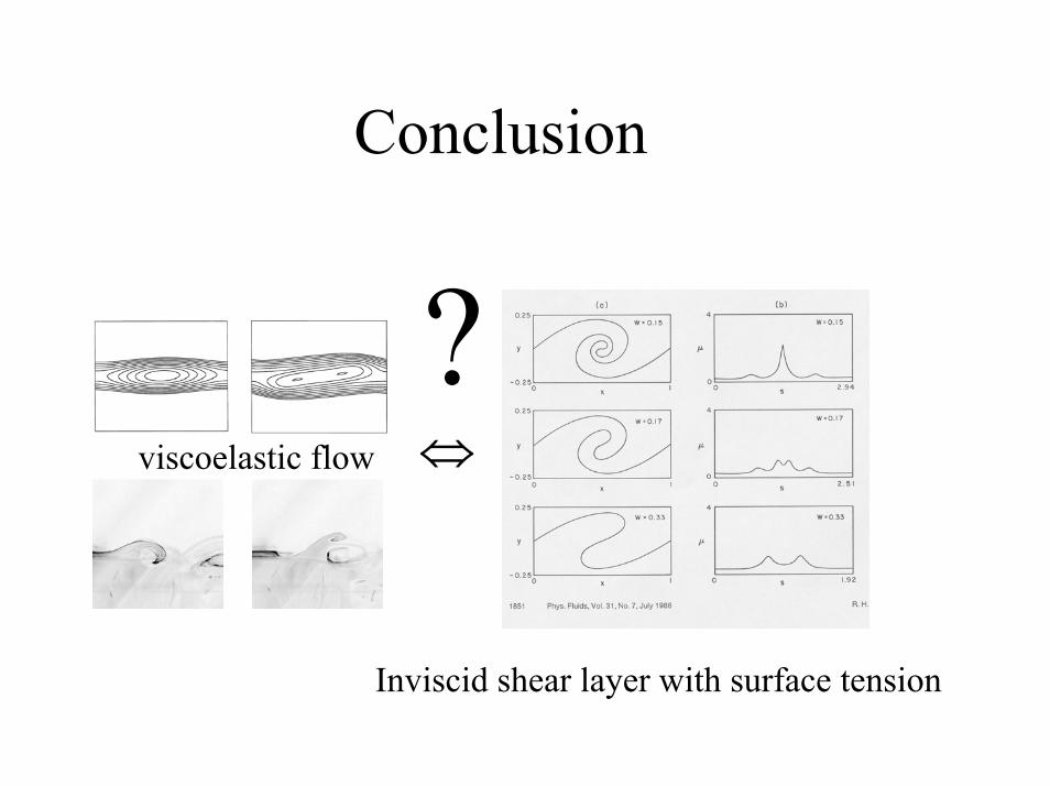
Conclusion

viscoelastic flow

Inviscid shear layer with surface tension

?⇔