Frequency Response and Filtering

6.003: Signal Processing

Frequency Response and Filtering

• Discrete-Time Frequency Response

• Continuous-Time Frequency Response

October 14, 2021

Context: The System Abstraction

Describe a system (physical, mathematical, or computational) by the way

it transforms an input signal into an output signal.

systemsignal

in

signal

out

This abstraction is particularly powerful for linear and time-invariant sys-

tems, which are both prevalent and mathematically tractable.

Three important representations for LTI systems:

• Difference/Differential Eq: algebraic input/output constraint√

• Convolution: represent system by unit-sample/impulse response√

• Filter: represent a system by its frequency response

Representing Systems with Difference/Differential Equations

Discrete-time systems that can be described by linear difference equations

with constant coefficients are linear and time-invariant.

LTIx[n] y[n]

∑l

cly[n−l] =∑m

dmx[n−m]

Continuous-time systems that can be described by linear differential equa-

tions with constant coefficients are linear and time-invariant.

LTIx(t) y(t)

∑l

cldly(t)dtl

=∑m

dmdmx(t)dtm

– natural and compact representations of many systems




systemsignal

in

signal

out







Unit-Sample Response and Impulse Response

Discrete-time systems that are linear and time-invariant can be completely

specified by their response to a unit-sample signal.

LTIx(t) y(t)

If δ[n]→ h[n], then x[n]→ y[n] = (x ∗ h)[n] =∑m

x[m]h[n−m]

Continuous-time systems that are linear and time-invariant are completely

specified by their response to a unit impulse function.

systemsignal

in

signal

out

If δ(t)→ h(t), then x(t)→ y(t) = (x ∗ h)(t) =∫x(τ)h(t− τ)dτ

– an LTI system is completely characterized by a single signal

Unit-Sample Response

The unit-sample response is a complete description of a system.

LTIδ[n] h[n]

This is a bit surprising since δ[n] is such a simple signal.

The unit-sample signal is the shortest possible non-trivial DT signal!

n

δ[n]→

n

h[n]

The response to this simple signal determines the response to any other

input signal:

x[n]→ y[n] = (x ∗ h)[n] =∑m

x[m]h[n−m]




systemsignal

in

signal

out







Frequency Response

The frequency response is a third way to characterize a linear time-

invariant system. This characterization is based on responses to sinusoids.

LTIcos(Ωn) A cos(Ωn+ φ)

n

cos(Ωn)

→ n

A cos(Ωn+ φ)

The idea is to characterize a system by the way A and φ vary with Ω.

Sinusoids differ from the unit-sample signal in important ways:

• eternal (longest possible signals) versus transient (shortest possible)

• comprises a single frequency versus a sum of all possible frequencies

Frequency Response

Using complex exponentials to characterize the frequency response.

LTIejΩn AejΩn

Notice that the complex valued A can represent both amplitude and phase.

We can find A using convolution.

y[n] = (x ∗ h)[n] =∞∑

m=−∞x[n−m]h[m] =

∞∑m=−∞

ejΩ(n−m)h[m]

= ejΩn∞∑

m=−∞h[m]e−jΩm = H(Ω) ejΩn

The response to a complex exponential is a complex exponential with the

same frequency but possibly different amplitude and phase.

The map for how a system modifies the amplitude and phase of a complex

exponential input is the Fourier transform of the unit-sample response.

Frequency Response

The frequency response is a complete characterization of an LTI system.

1. One can always find the frequency response of a system.

LTIejΩn H(Ω)ejΩn

2. Scaling the input by a constant scales the output by the same constant.

LTIX(Ω)ejΩn X(Ω)H(Ω)ejΩn

3. Linearity implies that the response to a sum is the sum of the responses.

LTIx[n] = 12π∫

2πX(Ω)ejΩndΩ y[n] = 12π∫

2πX(Ω)H(Ω)ejΩndΩ

4. The Fourier transform of the output is X(Ω)H(Ω).

LTIX(Ω) X(Ω)H(Ω)

The transform of the output is H(Ω) times the transform of the input.

Frequency Response

The frequency response is a complete description of a system.

LTIejΩn H(Ω)ejΩn

This is a bit surprising since ejΩn contains a single frequency.

→ can find the output of a system by breaking the input into its constituent

frequencies and summing the responses to each frequency – one-at-a-time.

n

cos(Ωn)

→ n

A cos(Ωn+ φ)

The frequency response can be used to find response to any input signal:

X(Ω)→ Y (Ω) = H(Ω)X(Ω)

Frequency Response

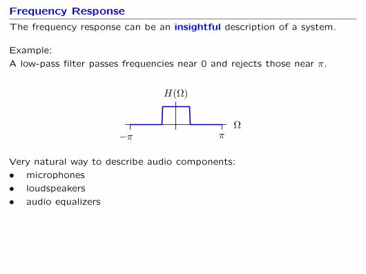
The frequency response can be an insightful description of a system.

Example:

A low-pass filter passes frequencies near 0 and rejects those near π.

Ω

H(Ω)

−π π

Very natural way to describe audio components:

• microphones

• loudspeakers

• audio equalizers

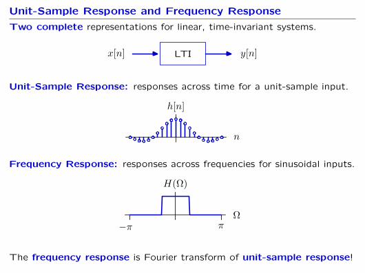
Unit-Sample Response and Frequency Response

Two complete representations for linear, time-invariant systems.

LTIx[n] y[n]

Unit-Sample Response: responses across time for a unit-sample input.

n

h[n]

Frequency Response: responses across frequencies for sinusoidal inputs.

Ω

H(Ω)

−π π

The frequency response is Fourier transform of unit-sample response!

Example

Find the frequency response of a system described by the following:

y[n]− αy[n−1] = x[n]

Example


y[n]− αy[n−1] = x[n]

Method 1:

Find the unit-sample response and take its Fourier transform.

h[n]− αh[n− 1] = δ[n]Solve the difference equation for h[n].

h[n] = δ[n] + αh[n−1]First order → need one initial condition: h[−1] = 0h[0] = δ[0] +αh[−1] = 1h[1] = δ[1] + αh[0] = α

h[2] = δ[2] + αh[1] = α2

h[3] = δ[3] + αh[2] = α3

h[n] = αnu[n]

H(Ω) =∞∑

n=−∞h[n]e−jΩn =

∞∑n=0

αne−jΩn =∞∑n=0

(αe−jΩ

)n= 1

1−αe−jΩ

Example


y[n]− αy[n−1] = x[n]

Method 2:

Find the response to ejΩn directly.

x[n] = ejΩn

Because the system is linear and time-invariant, the output will have the

same frequency as the input, but possibly different amplitude and phase.

y[n] = H(Ω)ejΩn

y[n−1] = H(Ω)ejΩ(n−1) = H(Ω)e−jΩejΩn

Substitute into the difference equation.

H(Ω)ejΩn − αH(Ω)e−jΩejΩn = H(Ω)(1−αe−jΩ)ejΩn = ejΩn

Since ejΩn is never 0, we can divide it out.

H(Ω) = 11− αe−jΩ

Same answer as method 1.

Example


y[n]− αy[n−1] = x[n]

Method 3:

Take the Fourier transform of the difference equation.

Y (Ω)− αe−jΩY (Ω) = X(Ω)Solve for Y (Ω).

Y (Ω) = 11− αe−jΩX(Ω)

Since Y (Ω) = H(Ω)X(Ω),

H(Ω) = 11− αe−jΩ

Same answer as methods 1 and 2.

Example

Plot the frequency response.

H(Ω) = 11−αe−jΩ

Note that denominator is the difference of 2 complex numbers.

If 0 < α < 1 :

Re

Im

1−Ω

green arrow: 1blue arrow: αe−jΩ

red arrow: 1− αe−jΩ

Ω

|H(Ω)|

2π−2π

11−α

11+α Ω

∠H(Ω)

2π

π/2

−π/2

Amplifies at low frequencies and attenuates high frequencies. Adds delay.

Check Yourself

Find the frequency response of a three-point averager:

y[n] = 13

(x[n−1] + x[n] + x[n+1]

)

n

x[n]

n

y[n]

The System Abstraction

The system abstraction applies equally well for continuous-time signals.

The System Abstraction



systemsignal

in

signal

out




• Differential Equation: algebraic constraint on derivatives√

• Convolution: represent a system by its impulse response√


Representing Systems with Difference/Differential Equations

Discrete-time systems that can be described by linear difference equa-

tions with constant coefficients are linear and time-invariant.

LTIx[n] y[n]

∑l

cly[n−l] =∑m

dmx[n−m]

Continuous-time systems that can be described by linear differential

equations with constant coefficients are linear and time-invariant.

LTIx(t) y(t)

∑l

cldly(t)dtl

=∑m

dmdmx(t)dtm

– natural and compact representations of many systems

Unit-Sample Response and Impulse Response

Discrete-time systems that are linear and time-invariant can be completely

specified by their response to a unit-sample signal.

LTIx[n] y[n]

If δ[n]→ h[n], then x[n]→ y[n] = (x ∗ h)[n] =∑m

x[m]h[n−m]

Continuous-time systems that are linear and time-invariant are completely

specified by their response to a unit impulse function.

LTIx(t) y(t)

If δ(t)→ h(t), then x(t)→ y(t) = (x ∗ h)(t) =∫x(τ)h(t− τ)dτ

– an LTI system is completely characterized by a single signal

Impulse Response

The impulse response is a complete description of a system.

LTIδ(t) h(t)

This is a bit surprising since δ(t) is zero almost everywhere.

The impulse function is the shortest possible non-trivial CT signal!

t

δ(t)→

t

h(t)

The response to this signal determines the response to any other input.

x(t)→ y(t) = (x ∗ h)(t) =∫x(τ)h(t−τ)dτ

Frequency Response

The frequency response is a third way to characterize a linear time-

invariant system. This characterization is based on responses to sinusoids.

LTIcos(ωt) A cos(ωt+ φ)

t

cos(ωt)

→ t

A cos(ωt+ φ)

The idea is to characterize a system by the way A and φ vary with ω.

Sinusoids differ from the unit-sample signal in important ways:

• eternal (longest possible signals) versus transient (shortest possible)

• comprises a single frequency versus a sum of all possible frequencies

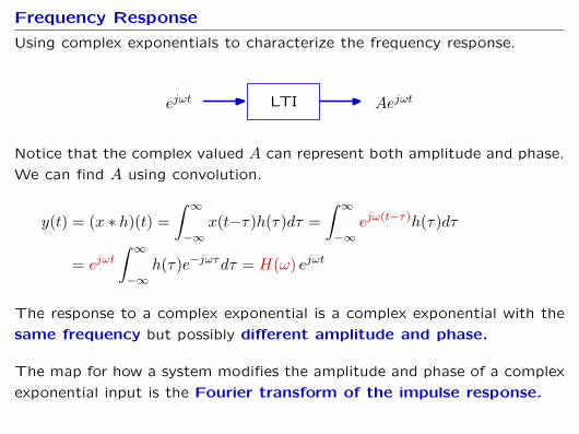
Frequency Response

Using complex exponentials to characterize the frequency response.

LTIejωt Aejωt

Notice that the complex valued A can represent both amplitude and phase.

We can find A using convolution.

y(t) = (x ∗ h)(t) =∫ ∞−∞

x(t−τ)h(τ)dτ =∫ ∞−∞

ejω(t−τ)h(τ)dτ

= ejωt∫ ∞−∞

h(τ)e−jωτdτ = H(ω) ejωt

The response to a complex exponential is a complex exponential with the

same frequency but possibly different amplitude and phase.

The map for how a system modifies the amplitude and phase of a complex

exponential input is the Fourier transform of the impulse response.

Frequency Response

The frequency response is a complete characterization of an LTI system.

1. One can always find the frequency response of a system.

systemejωt H(ω)ejωt

2. Scaling the input by a constant scales the output by the same constant.

systemX(ω)ejωt X(ω)H(ω)ejωt

3. Linearity implies that the response to a sum is the sum of the responses.

system12π∫∞−∞X(ω)ejωtdω 1

2π∫∞−∞X(ω)H(ω)ejωtdω

4. The Fourier transform of the output is X(ω)H(ω).

systemX(ω) X(ω)H(ω)

The transform of the output is H(ω) times the transform of the input.

Frequency Response

The frequency response is a complete description of a system.

LTIejωt H(ω)ejωt

This is a bit surprising since ejωt contains a single frequency.

→ can find the output of a system by breaking the input into its constituent

frequencies and summing the responses to each frequency – one-at-a time.

t

cos(ωt)

→ t

A cos(ωt+ φ)

The frequency response can be used to find response to any input signal:

X(ω)→ Y (ω) = H(ω)X(ω)

Frequency Response

The frequency response can be an insightful description of a system.

Example:

A low-pass filter passes frequencies near 0 and rejects those far from 0.

ω

H(ω)

Very natural way to describe audio enhancements:

• microphones

• loudspeakers

• audio equalizers

System Abstraction

Two complete representations for linear, time-invariant systems.

systemsignal

in

signal

out

Impulse Response: responses across time for a inpulse input.

t

h(t)

Frequency Response: responses across frequencies for sinusoidal inputs.

ω

H(ω)

The frequency response is Fourier transform of impulse response!

Example


y(t) + αdy(t)dt

= x(t)

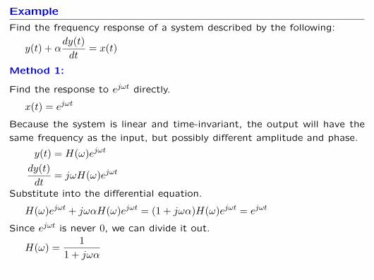
Example


y(t) + αdy(t)dt

= x(t)

Method 1:

Find the response to ejωt directly.

x(t) = ejωt

Because the system is linear and time-invariant, the output will have the

same frequency as the input, but possibly different amplitude and phase.

y(t) = H(ω)ejωt

dy(t)dt

= jωH(ω)ejωt

Substitute into the differential equation.

H(ω)ejωt + jωαH(ω)ejωt = (1 + jωα)H(ω)ejωt = ejωt

Since ejωt is never 0, we can divide it out.

H(ω) = 11 + jωα

Example


y(t) + αdy(t)dt

= x(t)

Method 2:

Take the Fourier transform of the differential equation.

Y (ω) + jωαY (ω) = X(ω)Solve for Y (ω).

Y (ω) = 11 + jωα

X(ω)

Since Y (ω) = H(ω)X(ω),

H(ω) = 11 + jωα

Same answer as method 1.

Example

Plot the frequency response.

H(ω) = 11 + jωα

Note that denominator is sum of 2 complex numbers.

Re

Im

1

jωα1+jωα

ω

|H(ω)|

10−10

1

ω

∠H(ω)

−10 10

π/2

−π/2

Amplifies low frequencies, attenuates high frequencies, adds phase delay.

Check Yourself

Find the frequency response of a rectangular box filter:

y(t) = 12

∫ t+1

t−1x(τ)dτ

(This CT filter is analogous to the three-point averager in DT.)

Summary

The Fourier transform of the response of a DT LTI system is the product of

the Fourier transform of the input times the system’s frequency response.

LTIX(Ω) Y (Ω)

Y (Ω) = H(Ω)X(Ω)

The frequency response H(Ω) is the Fourier transform of the unit-sample

response h[n].

The Fourier transform of the response of a CT LTI system is the product of

the Fourier transform of the input times the system’s frequency response.

LTIX(ω) Y (ω)

Y (ω) = H(ω)X(ω)

The frequency response H(ω) is the Fourier transform of the impulse re-

sponse h(t).

Documents

Frequency Response and Filtering