Frequent Closed Pattern Search By Row and Feature Enumeration

Outline Problem Definition

Related Work: Feature Enumeration Algorithms

CARPENTER: Row Enumeration Algorithm

COBBLER: Combined Enumeration Algorithm

Problem Definition Frequent Closed Pattern:

1) frequent pattern: has support value higher than the threshold

2) closed pattern: there exists no superset which has the same support value

Problem Definition:Given a dataset D which contains records consist of features, our problem is to discover all frequent closed patterns respect to a user defined support threshold.

Related Work

Searching Strategy:breadth-first & depth-first search

Data Format:horizontal format & vertical format

Data Compression Method:diffset, fp-tree, etc.

Typical Algorithms APRIORI

feature enumeration horizontal format breadth-first search

CHARM feature enumeration vertical format depth-first search deffset technique

CLOSET feature

enumeration horizontal format depth-first search fp-tree technique

CARPENTERCARPENTER stands for Closed Pattern Discovery by Transposing Tables that are Extremely Long

Motivation

Algorithm

Prune Method

Experiment

Motivation Bioinformatic datasets typically contain large

number of features with small number of rows.

Running time of most of the previous algorithms will increase exponentially with the average length of the transactions.

CARPENTER’s search space is much smaller than that of the previous algorithms on these kind of datasets and therefore has a better performance.

Algorithm

The main idea of CARPENTER is to mine the dataset row-wise.

2 steps: First, transpose the dataset Second , search in the row enumeration tree.

Transpose Table Feature a, b, c, d. Row r1, r2 , r3, r4.

r1 a b c

r2 b c d

r3 b c d

r4 d

a r1

b r1 r2 r3

c r1 r2 r3

d r2 r3 r4

original table transposed table

transpose

b

c

d r4project on (r2 r3)

projected table

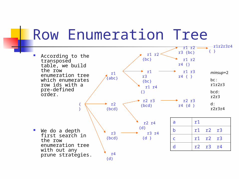
Row Enumeration Tree According to the

transposed table, we build the row enumeration tree which enumerates row ids with a pre-defined order.

We do a depth first search in the row enumeration tree with out any prune strategies.

{ }

r1 {abc}

r2 {bcd}

r3 {bcd}

r4 {d}

r1 r2 {bc}

r1 r3 {bc}

r1 r4 {}

r1 r2 r3 {bc}

r1 r2 r4 {}

r1 r3 r4 { }

r2 r3 {bcd}

r2 r4 {d}

r2 r3 r4 {d }

r3 r4 {d }

r1r2r3r4 { }

minsup=2

bc: r1r2r3

bcd: r2r3

d: r2r3r4

a r1

b r1 r2 r3

c r1 r2 r3

d r2 r3 r4

Prune Method 1 In the

enumeration tree, the depth of a node is the corresponding support value.

Prune a branch if there won’t be enough depth in that branch, which means the support of patterns found in the branch will not exceed the minimum support.

r2 {bcd}

r2 r3 {bcd}

r2 r4 {d}

depth= 1

sup =1

2 sub-nodes

Max support value in branch “r2” will be 3, therefore prune this branch.

minsup 4

Prune Method 2 If rj has 100% support in

projects table of ri, prune

the branch of rj.

b r3

c r3

d r3 r4

r2 {bcd} r2 r3 {bcd}

r2 r4 {d}

r3 has 100% support in the projected table of “r2”, therefore branch “r2 r3” will be pruned and whole branch is reconstructed.

r2 r3 r4 {d}

r2 r3 {bcd} r2 r3 r4 {d}

b

c

d r4

Prune Method 3 At any node in

the enumeration tree, if the corresponding itemset of the node has been found before, we prune the branch rooted at this node.

r2 {bcd} r2 r3 {bcd}

r2 r4 {d}

r3 {bcd} r3 r4 {d}

Since itemset {bcd} has been found before, the branch rooted at “r3” will be pruned.

Performance We compare 3 algorithms,

CARPENTER, CHARM and CLOSET.

Dataset (Lung Cancer) has 181 rows with 12533 features.

We set 3 parameters, minsup, Length Ratio and Row Ratio.

minsupLung Cancer, 181 rows, length ratio 0.6,row ratio 1.

Running time of CARNPENTER changes from 3 to 14 second

0.1

1

10

100

1000

10000

100000

4 5 6 7 8 9 10

minsup

Run

time

(sec

.)

carpenter (sec)charm (sec)closet (sec)

Length RatioLung Cancer, 181 rows, sup 7 (4%), row ratio 1

Running time of CARPENTER changes from 3 to 33 seconds

1

10

100

1000

10000

100000

0.3 0.4 0.5 0.6 0.7 0.8 0.9 1

Length Ratio

Ru

nti

me

(sec

.)

carpenter (sec)charm (sec)closet (sec)

Row RatioLung Cancer, 181 rows, length ratio 0.6,sup 7 (4%)

Running time of CARPENTER changes from 9 to 178 seconds

1

10

100

1000

10000

0 1 2 3 4 5 6

Row Ratio

Ru

nti

me

(sec

.)

carpenter (sec)charm (sec)closet (sec)

Conclusion We propose an algorithm call CARPENTER for

finding closed pattern on long biological datasets.

CARPENTER perform row enumeration instead of column enumeration since the number of rows in such datasets are significantly smaller than the number of features.

Performance studies show that CARPENTER is much more efficient in finding closed patterns compared to existing feature enumeration algorithms.

COBBLER

Motivation

Algorithm

Performance

Motivation With the development of CARPENTER,

existing algorithms can be separated into two parts. Feature enumeration: CHARM, CLOSET, etc. Row enumeration: CARPENTER

We have two motivations to combine these two enumeration methods

Motivation1. We can see that these two enumeration methods have

their own advantages on different type of data set. Given a dataset, the characteristic of its sub-dataset may change.

2. Given a dataset with both large number of rows and features, a single row enumeration algorithm or a single feature enumeration method can not handle the dataset.

dataset

sub-dataset

more rows than features more features than rows

project

Algorithm There are two main points in the

COBBLER algorithm How to build an enumeration tree for

COBBLER. How to decide when the algorithm should

switch from one enumeration to another.

Therefore, we will introduce the idea of dynamic enumeration tree and switching condition

Dynamic Enumeration Tree We call the new kind of enumeration tree used

in COBBLER the dynamic enumeration tree. In dynamic enumeration tree, different sub-tree

may use different enumeration method.

We use the table as an example in later discussion

r1

a b c

r2

a c d

r3

b c

r4

d

a r1 r2

b r1 r3

c r1 r2 r3

d r2 r4

original transposed

{ }

a {r1r2}

b {r1r3}

c {r1r2r3}

d {r2r4

}

ab {r1}

ac {r1r2}

ad {r2}

abc {r1}

abd { }

acd { r2}

bc {r1r3}

bd { }

bcd { }

cd {r2 }

{ }

r1 {abc}

r2 {acd}

r3 {bc}

r4 {d}

r1r2 {ac}

r1r3 {bc}

r1r4 { }

r1r2r3 {c}

r1r2r4 { }

r1r3r4 { }

r2r3 {c}

r2r4 {d }

r2r3r4 { }

r3r4 { }

Single Enumeration Tree r1r2r3r4

{ } abcd

{ }

Feature enumeration Row enumeration

r1 a b c

r2 a c d

r3 b c

r4 d

Dynamic Enumeration Tree

{ }

a {r1r2}

b {r1r3}

c {r1r2r3}

d {r2r4

}

r1 {bc}

r2 {cd}

r1r2 {c}

r1 {c}

r3 { c}

r1r3 { c}

r2 {d }

Feature enumeration to Row enumeration

ab {r1}

ac {r1r2}

ad {r2}

abc {r1}

abd { }

acd { r2}

abcd { }

a {r1r2}

abc: {r1}

ac: {r1r2}

acd: {r2}

r1

bc

r2

cd

b r1

c r1 r2

d r2

Dynamic Enumeration Tree

{ }

r1 {abc}

r2 {acd}

r3 {bc}

r4 {d}

a {r2}

b {r3}

c {r2r3 }

ab {}

ac { r2}

bc {r3 }

a {r1}

d {r4 }

ac {r1 }

b {r1 }

Row enumeration to Feature Enumeration

c {r1r3}

ad { }

acd { }

cd { }

c {r1r2 }

bc {r1 }

r1 {abc}

r1r2 {ac}

r1r3 {bc}

r1r4 { }

r1r2r3 {c}

r1r2r4 { }

r1r3r4 { }

r1r2r3r4 { }

ac: {r1r2}

bc: {r1r3}

c: {r1r2r3}

Dynamic Enumeration Tree When we use different condition to decide the

switching, the structure of the dynamic enumeration tree will change.

No matter how it switches, the result set of closed pattern will be the same as the result of

the single enumeration .

Switching Condition The main idea of the switching condition is to

estimate the processing time of the a enumeration sub-tree, i.e., row enumeration sub-tree or feature enumeration sub-tree.

Define some characters.

Switching Condition

f1 f2 f3 fn

{f1,f2} {f1,fn}...

{f1,f2,f3}...

{f1,f2..fp}Deepest node

under f1

{f2,f3} {f2,fn}...

{f2,f3,f4} ...

{f2..fq}Deepest node

under f2

{f3,f4} {f3,fn}...

.

.

.

{f3..fk}Deepest node

under f3

{f3,f4,f5}

... f1 f2 f3 fn

{f1,f2}

.

.

.

{f1,f2..fp}Deepest node

under f1

{f2,f3}

.

.

.

{f2..fq}Deepest node

under f2

{f3,f4}

.

.

.

{f3..fk}Deepest node

under f3

...

Switching Condition

Suppose r=10, S(f1)=0.8, S(f2)=0.5, S(f3)=0.5, S(f4)=0.3 and minsup=2

Then the estimated deepest node under f1 is f1f2f3, since S(f1)*S(f2)*S(f3)*r=2 >minsup S(f1)*S(f2)*S(f3)*S(f4)*r=0.6 < minsup

Experiments We compare 3 algorithms,

COBBLER, CHARM and CLOSET+.

One real-life dataset and one synthetic data.

We set 3 parameters, minsup, Length Ratio and Row Ratio.

minsup

0

5000

10000

15000

20000

25000

30000

35000

40000

14% 16% 18% 20%

Minimum Support

Ru

nti

me

(sec

.)

COBBLER

CLOSET+

CHARM

0

1000

2000

3000

4000

5000

6% 8% 10% 12% 14% 16%

Minimum Support

Ru

nti

me

(s

ec

.)

COBBLER

CLOSET+

CHARM

Synthetic data Real-life data (thrombin)

Length and Row ratio

0

2000

4000

6000

8000

10000

12000

14000

0.75 0.8 0.85 0.9 0.95 1 1.05

Length Ratio

Ru

nti

me

(sec

.)

COBBLER

CLOSET+

CHARM

0

10000

20000

30000

40000

50000

60000

70000

80000

0.5 1 1.5 2

Row Ratio

Ru

nti

me

(sec

.)

COBBLER

CLOSET+

CHARM

Synthetic data

Discussion The combination of row and feature

enumeration also makes some disadvantage

The cost to calculate the switching condition and the cost of bad decision.

The increased cost in pruning, maintain two set of pruning system.

Discussion We may use other more complicated

data structure in our algorithm to improve the performance, e.g., the vertical data format and diffset technique.

And more efficient switching condition may improve the algorithm further.

Conclusion The COBBLER algorithm gives better

performance on dataset where the advantage of switching can be shown, e.g., complex dataset or dataset has both large number of rows and features.

For simple characteristic data, a single enumeration algorithm may be better.

Future Work

Using other data structure and technique in the algorithm.

Extend COBBLER to handle dataset that can not be fitted into memory.

Thanks