WAIRESEARCH LIMITED

Freshwater fish predictive modelling for

bioassessment;

A scoping study into fish bioassessment models as national indicators

in New Zealand

Mike Joy

January 2013

1 | P a g e

TABLE OF CONTENTS

Executive summary ......................................................................................................................................................... 2

Introduction ........................................................................................................................................................................ 3

Methods ................................................................................................................................................................................ 5

Fish data ...................................................................................................................................................................... 5

Land cover data - river environment classification (REC) ..................................................................... 6

Predictive spatial models .................................................................................................................................... 6

Calculating observed over expected O/E ratios ......................................................................................... 6

Best probability thresholds ................................................................................................................................ 6

Index of biotic integrity (IBI) ............................................................................................................................. 7

Results ................................................................................................................................................................................... 8

Observed over expected ratios .......................................................................................................................... 8

validation using the river environment classification .......................................................................... 10

Discussion ......................................................................................................................................................................... 16

Conclusions & Recommendations .......................................................................................................................... 17

References ........................................................................................................................................................................ 20

2 | P a g e

EXECUTIVE SUMMARY The match between the biota expected at a site in the absence of impacts and what is found

there when testing is a robust and popular bioassessment method in many countries worldwide.

The difference between the assemblage found and that expected is measured as the

observed/expected ratio and is the basis of the RIVPACS1 approach initially developed in the

United Kingdom using invertebrates.

When the observed and expected assemblages match the O/E score is 1. An O/E score less than

1 means some impact and more than 1 suggests better than expected biota.

This scoping trial of the feasibility of a fish predictive RIVPACS type bioassessment using the New

Zealand Freshwater Fish Database (NZFFDB) and predictive models of fish distribution from the

Freshwater Ecosystems of New Zealand2 (FENZ) was not successful.

This study revealed that the predictive bioassessment approach in this case failed mainly due to

the lack of suitable predictive models for this not because of problems with the predictive

bioassessment approach.

The problem with the available FENZ fish predictions used ij this study is that they were

developed to predict how the fish assemblages are today allowing for many land-use impacts

rather than the predictions of the assemblages that would be expected in the absence of

impacts crucial to RIVPACS type models.

Regional O/E fish models have been successfully applied with fish in New Zealand by taking all

the steps in the RIVPACS process but have generally not been taken up by resource managers.

To validate the data used in this study an Index of Biotic Integrity (IBI) was successfully applied to

the observed (NZFFDB) and predicted fish assemblages (FENZ) and revealed their suitability for

bioassessment.

However, an assessment of the observed/expected IBI results was, like the fish community O/E

unsuccessful, again because the predictions are for actual rather than expected fish

communities.

1 This is the River Invertebrate Prediction and Classification System, first developed in the United Kingdom in 1984/ 2 http://www.doc.govt.nz/conservation/land-and-freshwater/freshwater/freshwater-ecosystems-of-new-zealand/

3 | P a g e

The conclusions from this study are that predictive bioassessment models have great potential

for use in New Zealand but there are no shortcuts. Consequently, new predictive models must

be produced based on reference sites and using habitat descriptors that are least influenced by

human impacts.

In the meantime the IBI is a useful measure of the biotic integrity of freshwater in New Zealand,

and improvements in sampling and metrics to take into account abundance and size/age classes

show that the IBI can be updated and the outputs precision improved.

INTRODUCTION

FISH IN BIOASSESSMENT

Freshwater biological communities are sensitive indicators of the relative health of their ecosystems

and the surrounding catchment (Fausch et al. 1990, McCormick et al. 2000). The relationship

between the biological, physical and chemical components of ecosystems is the basis of biological

monitoring. Fish are potentially effective indicators of the condition of aquatic ecosystems, because

different species exhibit diverse ecological, morphological and behavioural adaptations to their

natural habitat (Karr et al. 1986, Fausch et al. 1990). Fish communities integrate the ecological

processes of streams across both temporal and spatial scales (Karr et al. 1986, Fausch et al. 1990),

therefore they can be useful indicators of aquatic degradation (Karr 1981, Karr 1991b, a).

Furthermore, because fish are a visible part of stream biological integrity, they represent a measure

of stream quality easily and intuitively understood by the public (McCormick et al. 2000).

Despite this potential however, until recently fish were seldom used in biological assessment in New

Zealand because of the overwhelming influence of altitude and distance from the sea on fish

distribution (Joy et al. 2000, McDowall and Taylor 2000, Joy and Death 2001). The development in

2004 of a fish index of biotic integrity (IBI) (Joy and Death 2004a) resulted in national and regional

freshwater fish integrity analyses in relation to land use and temporal trends (Joy 2009), and many

regional councils (Southland, Tasman, Waikato, Auckland, Hawkes Bay and Wellington) now have

regional IBI models for use in state of the environment and other monitoring e.g. (Joy 2005b, 2008).

4 | P a g e

BACKGROUND TO SCOPING STUDY

This assessment was undertaken to investigate the feasibility of using freshwater fish predictive

models in national bioassessment in New Zealand. Although regional predictive bioassessment

models have been developed (Joy and Death 2000, 2002b, a) they have rarely been used in

bioassessment and being regional are not suitable for national assessment. The main objective of

this scoping study was to see if the existing extensive database of fish distribution (the New Zealand

freshwater fish database) could be combined with an existing national predictive model of fish

distribution (Leathwick et al. 2008a) to give a baseline measure of fish communities at a national

scale.

This study was undertaken with the recognition that many of the requirements of the predictive

bioassement models developed and used overseas would not be met, but given the lack of resources

and time to address these issues an assessment of its potential use could be made with the existing

data. The limitations included the lack of ‘reference site’(Kennard et al. 2006, Robertson et al. 2006,

Wang et al. 2008) data and the fact that the predictions used are predictions for how the

communities are now including impacts not how they would be in the absence of those impacts.

EXPECTATIONS OF SCOPING STUDY

The advantage of using predictions that include all sites (not just reference sites) and human-

influenced variables is that the predictions are more accurate, as there is always a trade-off between

accuracy of predictive models and limiting predictions by removing sites and variables. The

hypothesis in this case was that using the large number of sites in the database the O/E scores would

represent baseline conditions and that the upper and lower ends of the distribution of scores would

represent extremely good and extremely bad sites respectively. It was anticipated that the upper

end of the range of O/E score would include many of the sites in native vegetation and not many

sites in developed catchments as a validation of the method.

PREDICTIVE MODELS IN BIOASSESSMENT

The basis of the analysis assessed in this report is the River Invertebrate Prediction and Classification

System (RIVPACS) approach, originally developed in the U.K. by Wright and colleagues (Wright 1995)

later advanced by Simpson & Norris in Australia with the Australian River Assessment Scheme

5 | P a g e

(AUSRIVAS) (Simpson and Norris 2000) and more recently in the USA (Hargett et al. 2007, Carlisle

and Hawkins 2008, Yuan et al. 2008, Aguiar et al. 2011, Tsang et al. 2011). These predictive

bioassessment models are similar and will be referred to in this report as RIVPACS models. RIVPACS

models assess biological status by comparing the biotic condition at sites being evaluated with the

biota expected to occur in the absence of stress (Wright 1995). A detailed account of the

background to this type of predictive modelling has been covered in numerous publications e.g.

(Wright 1995, Hawkins et al. 2000, Simpson and Norris 2000, Joy and Death 2001), and hence will

not be explained in detail here. But a basic summary of the steps are:

1. A predictive model is built using biological, physical and chemical data collected at a number

of unimpacted or minimally impacted sites, generally referred to as reference sites.

2. The reference sites are classified into groups based on the homogeneity of their fauna, and

the physical and chemical characteristics that best describe variation among the groups are

determined.

3. Some form of discriminant analysis is used to predict the biotic communities expected to

occur in the absence of environmental stress.

4. Finally the expected community is defined as the sum of probabilities for all predicted

species and this is divided by the observed list of species (only if predicted to be there) to

give the observed over expected ratio.

In this assessment some of the steps described above were omitted or altered. The main differences

were: 1) the predictions did not come from reference sites and 2) the predictions included land use

and other human influenced variables so were effectively “how it is“ rather than “how it would be in

the absence of impact”.

METHODS

FISH DATA

All fish records were taken from the New Zealand Freshwater Fish Database (NZFFDB)

(McDowall and Richardson 1983, Richardson 1989, Richardson 1993) for the years 1970 – 2010

for all sampling methods which gave a total of 27300 sites. However, not all sites had

matching predictive fish or environmental data so approximately 27000 sites were analysed for

this project. Since this is a scoping study to trial different methods no attempt was made to

6 | P a g e

select database entries with different levels of sampling intensity or gear type, the assumption

was that a large number of sites would lessen the effects of sampling variability.

LAND COVER DATA - RIVER ENVIRONMENT CLASSIFICATION (REC)

The REC classifications were used to validate the O/E. The O/E and IBI scores for each database

record were associated with its REC classification (Snelder and Guest 2000, Snelder and Biggs 2002,

Snelder et al. 2002, Snelder et al. 2004).

PREDICTIVE SPATIAL MODELS

The predictive models used came from freshwater ecosystems of New Zealand (FENZ) project

(Leathwick et al. 2008b). As part of the FENZ, the spatial distribution of most fish species were

extended out over the entire river network was predicted using boosted regression trees by

John Leathwick. This technique known as fish mapping was first developed in New Zealand by

Joy and Death (Joy and Death 2004b). in this study, the predictive models for all fish species

were used, only native fish and trout were used for the O/E models, all non-native as well as

native for the IBI assessment.

CALCULATING OBSERVED OVER EXPECTED O/E RATIOS

The predicted fish assemblages from the Leathwick models were compared with the observed fish

assemblages using an O/E ratio following the procedure originally described by Wright et al. (1984).

To do this the following procedure was used: The probabilities of the predicted taxa were summed

to give the ‘expected number of taxa’ (E). The number of species actually captured at a site,

providing they were predicted to occur (and met the threshold used) was the ‘observed number of

taxa’ (O). The ratio of the observed to the expected number of taxa (O ⁄ E) is the output from the

model.

BEST PROBABILITY THRESHOLDS

Using the probabilities of occurrence from predictive models in bioassessment raises the issue of

deciding on the probability threshold to use. Many models use the 0.5 (or 50% probability

7 | P a g e

threshold) - so that a probability greater than 0.5 means the species is present and less than 0.5

means absence (Fielding and Bell 1997). This approach is acceptable if the data that were used to

create the model are balanced i.e. that the species modelled has a prevalence of around 50%, but in

the data set used in these models prevalence varied from 0.003 to 0.37 so the 0.5 or any single

threshold over all species would not give the best representation of the likelihood of finding it. To

circumvent this problem the threshold that gave the best prediction was found for each species.

This was done by trying all thresholds between 0 and 1 in 0.01 steps and then selecting the threshold

that gave the best overall prediction measured as the maximum Cohen’s Kappa (Cohen 1960, Olden

et al. 2006b).

INDEX OF BIOTIC INTEGRITY (IBI)

The Index of Biotic Integrity (IBI) was originally developed using fish in the USA by James Karr

during the early 1980s (Karr et al. 1986). The original version had 12 metrics that reflected fish

species richness and composition, number and abundance of indicator species, trophic

organization and function, reproductive behaviour, fish abundance, and condition of individual

fish. This process has been repeated and IBIs developed on many continents. The fish fauna

of New Zealand is however, radically different from the continental faunas thus the IBI

developed for New Zealand includes a number of changes see (Joy and Death 2004a) for full

details.

The six metrics that are used in the New Zealand IBI measure taxonomic richness over a number of

habitat guilds, and as well use indicator species by measuring the number of species showing

intolerance to degraded conditions and the ratio of native to exotic species. Many studies have

shown that New Zealand’s fish fauna is largely structured by elevation and distance from the coast

(McDowall 1988, McDowall 1990, Joy and Death 2001). Because elevation and distance from the

coast are the overriding controllers of native fish species distribution they were used to structure

expectations of fish assemblages. The six metrics were assessed for both elevation and distance

from the coast to give 12 metrics overall and these were summed to give the final score. IBI scores

were calculated for all the sites used in this study to compare with the O/E scores.

8 | P a g e

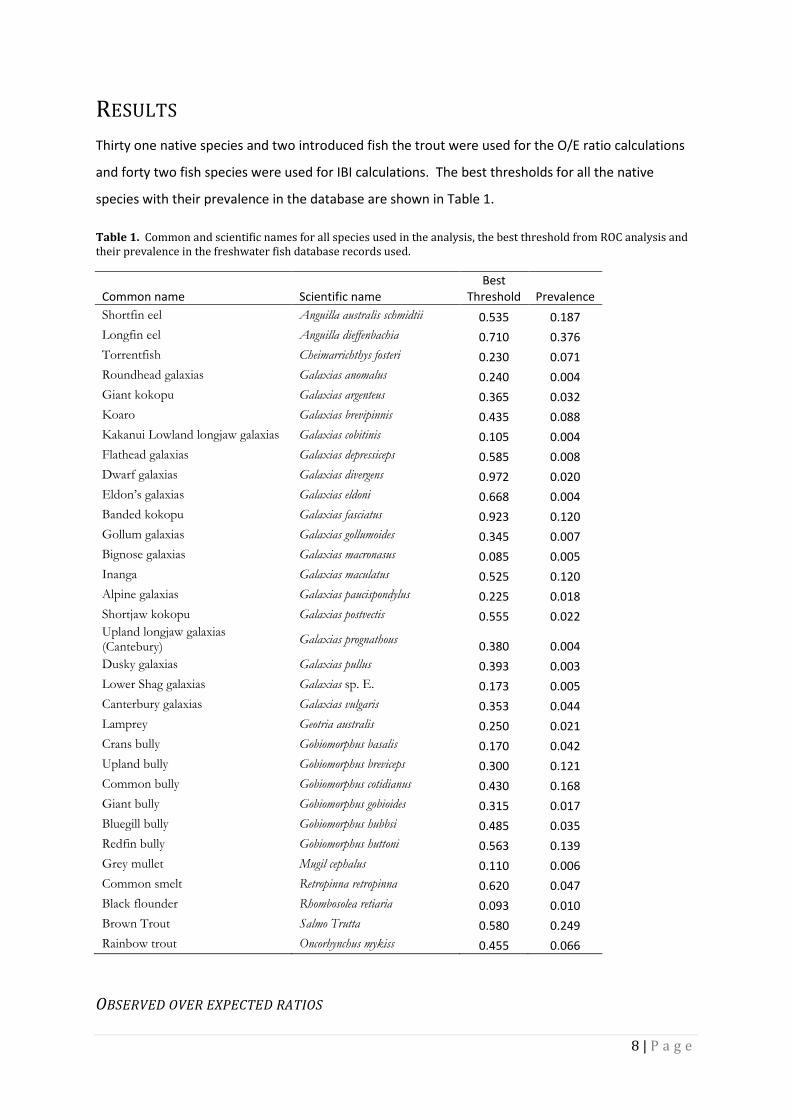
RESULTS

Thirty one native species and two introduced fish the trout were used for the O/E ratio calculations

and forty two fish species were used for IBI calculations. The best thresholds for all the native

species with their prevalence in the database are shown in Table 1.

Table 1. Common and scientific names for all species used in the analysis, the best threshold from ROC analysis and their prevalence in the freshwater fish database records used.

Common name Scientific name Best

Threshold Prevalence

Shortfin eel Anguilla australis schmidtii 0.535 0.187

Longfin eel Anguilla dieffenbachia 0.710 0.376

Torrentfish Cheimarrichthys fosteri 0.230 0.071

Roundhead galaxias Galaxias anomalus 0.240 0.004

Giant kokopu Galaxias argenteus 0.365 0.032

Koaro Galaxias brevipinnis 0.435 0.088

Kakanui Lowland longjaw galaxias Galaxias cobitinis 0.105 0.004

Flathead galaxias Galaxias depressiceps 0.585 0.008

Dwarf galaxias Galaxias divergens 0.972 0.020

Eldon’s galaxias Galaxias eldoni 0.668 0.004

Banded kokopu Galaxias fasciatus 0.923 0.120

Gollum galaxias Galaxias gollumoides 0.345 0.007

Bignose galaxias Galaxias macronasus 0.085 0.005

Inanga Galaxias maculatus 0.525 0.120

Alpine galaxias Galaxias paucispondylus 0.225 0.018

Shortjaw kokopu Galaxias postvectis 0.555 0.022 Upland longjaw galaxias (Cantebury)

Galaxias prognathous 0.380 0.004

Dusky galaxias Galaxias pullus 0.393 0.003

Lower Shag galaxias Galaxias sp. E. 0.173 0.005

Canterbury galaxias Galaxias vulgaris 0.353 0.044

Lamprey Geotria australis 0.250 0.021

Crans bully Gobiomorphus basalis 0.170 0.042

Upland bully Gobiomorphus breviceps 0.300 0.121

Common bully Gobiomorphus cotidianus 0.430 0.168

Giant bully Gobiomorphus gobioides 0.315 0.017

Bluegill bully Gobiomorphus hubbsi 0.485 0.035

Redfin bully Gobiomorphus huttoni 0.563 0.139

Grey mullet Mugil cephalus 0.110 0.006

Common smelt Retropinna retropinna 0.620 0.047

Black flounder Rhombosolea retiaria 0.093 0.010

Brown Trout Salmo Trutta 0.580 0.249

Rainbow trout Oncorhynchus mykiss 0.455 0.066

OBSERVED OVER EXPECTED RATIOS

9 | P a g e

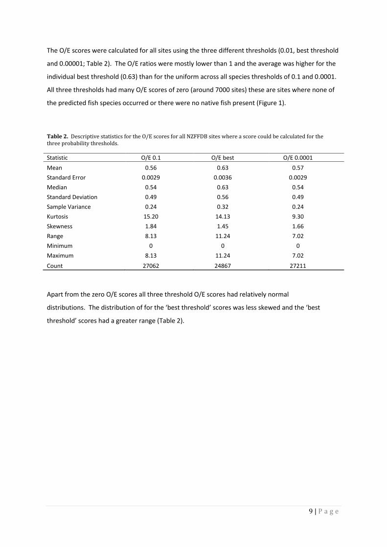
The O/E scores were calculated for all sites using the three different thresholds (0.01, best threshold

and 0.00001; Table 2). The O/E ratios were mostly lower than 1 and the average was higher for the

individual best threshold (0.63) than for the uniform across all species thresholds of 0.1 and 0.0001.

All three thresholds had many O/E scores of zero (around 7000 sites) these are sites where none of

the predicted fish species occurred or there were no native fish present (Figure 1).

Table 2. Descriptive statistics for the O/E scores for all NZFFDB sites where a score could be calculated for the three probability thresholds.

Statistic O/E 0.1 O/E best O/E 0.0001

Mean 0.56 0.63 0.57

Standard Error 0.0029 0.0036 0.0029

Median 0.54 0.63 0.54

Standard Deviation 0.49 0.56 0.49

Sample Variance 0.24 0.32 0.24

Kurtosis 15.20 14.13 9.30

Skewness 1.84 1.45 1.66

Range 8.13 11.24 7.02

Minimum 0 0 0

Maximum 8.13 11.24 7.02

Count 27062 24867 27211

Apart from the zero O/E scores all three threshold O/E scores had relatively normal

distributions. The distribution of for the ‘best threshold’ scores was less skewed and the ‘best

threshold’ scores had a greater range (Table 2).

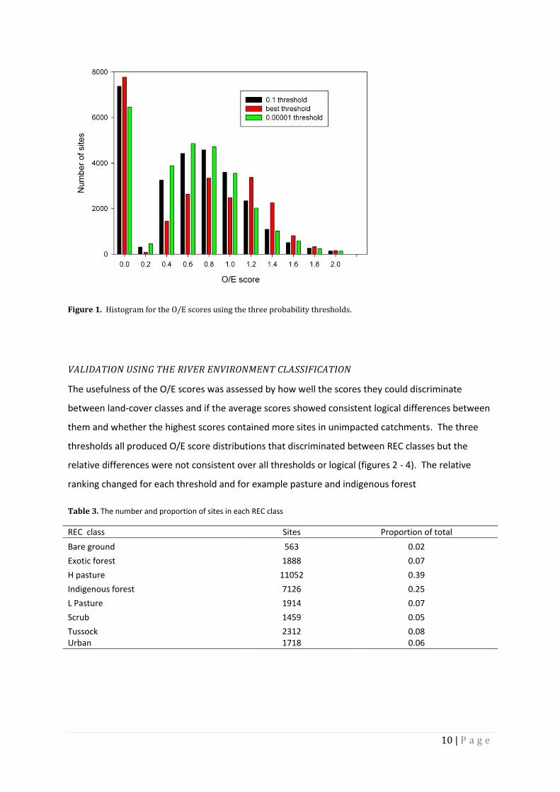
10 | P a g e

Figure 1. Histogram for the O/E scores using the three probability thresholds.

VALIDATION USING THE RIVER ENVIRONMENT CLASSIFICATION

The usefulness of the O/E scores was assessed by how well the scores they could discriminate

between land-cover classes and if the average scores showed consistent logical differences between

them and whether the highest scores contained more sites in unimpacted catchments. The three

thresholds all produced O/E score distributions that discriminated between REC classes but the

relative differences were not consistent over all thresholds or logical (figures 2 - 4). The relative

ranking changed for each threshold and for example pasture and indigenous forest

Table 3. The number and proportion of sites in each REC class

REC class Sites Proportion of total

Bare ground 563 0.02

Exotic forest 1888 0.07

H pasture 11052 0.39

Indigenous forest 7126 0.25

L Pasture 1914 0.07

Scrub 1459 0.05

Tussock 2312 0.08 Urban 1718 0.06

11 | P a g e

Figure 2. Average O/E score (± SE) for each REC class using the prediction threshold of 0.1. See table 3 for details on number of sites in each class

Figure 3. Average O/E score (± SE) for each REC class using the best prediction threshold. See table 3 for details on number of sites in each class

12 | P a g e

Figure 4. Average O/E score (± SE) for each REC class using the 0.00001 prediction threshold. See table 3 for details on number of sites in each class.

The next validation test was to take the higher scoring sites and see if the natural landcover classes

were better represented. All sites with an O/E score greater than 0.9 were compared with the

background distribution of O/E scores by land-cover class to see if there was a difference. The

comparison revealed no difference in the land-cover site distribution for the greater than 0.9 scores

(Figure 5). The O/E sores produced were not able to discriminate between land-cover and thus the

assessment showed the O/E methods failed.

Figure 5. The number of sites in each REC class for all sites (black bars) and sites with an O/E score > 0.9 (grey bars).

13 | P a g e

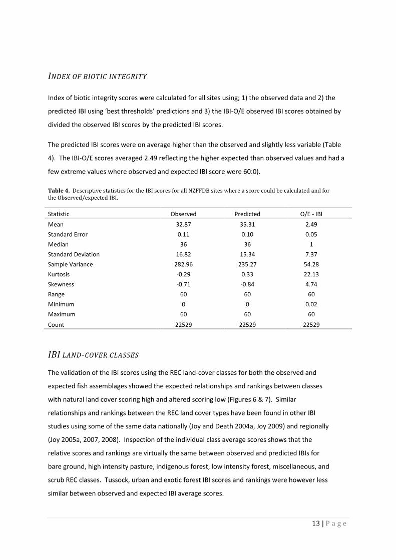
INDEX OF BIOTIC INTEGRITY

Index of biotic integrity scores were calculated for all sites using; 1) the observed data and 2) the

predicted IBI using ‘best thresholds’ predictions and 3) the IBI-O/E observed IBI scores obtained by

divided the observed IBI scores by the predicted IBI scores.

The predicted IBI scores were on average higher than the observed and slightly less variable (Table

4). The IBI-O/E scores averaged 2.49 reflecting the higher expected than observed values and had a

few extreme values where observed and expected IBI score were 60:0).

Table 4. Descriptive statistics for the IBI scores for all NZFFDB sites where a score could be calculated and for the Observed/expected IBI.

Statistic Observed Predicted O/E - IBI

Mean 32.87 35.31 2.49

Standard Error 0.11 0.10 0.05

Median 36 36 1

Standard Deviation 16.82 15.34 7.37

Sample Variance 282.96 235.27 54.28

Kurtosis -0.29 0.33 22.13

Skewness -0.71 -0.84 4.74

Range 60 60 60

Minimum 0 0 0.02

Maximum 60 60 60

Count 22529 22529 22529

IBI LAND-COVER CLASSES

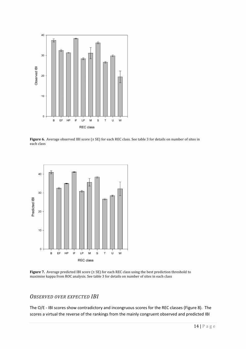
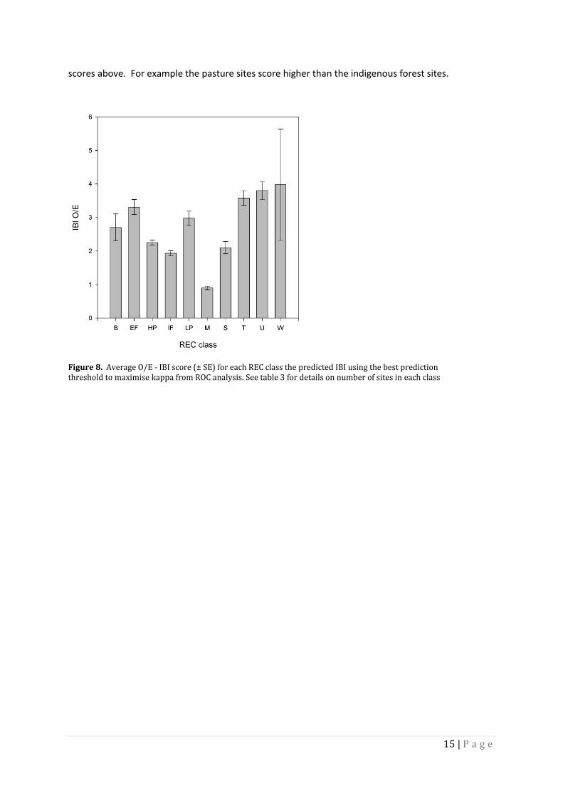
The validation of the IBI scores using the REC land-cover classes for both the observed and

expected fish assemblages showed the expected relationships and rankings between classes

with natural land cover scoring high and altered scoring low (Figures 6 & 7). Similar

relationships and rankings between the REC land cover types have been found in other IBI

studies using some of the same data nationally (Joy and Death 2004a, Joy 2009) and regionally

(Joy 2005a, 2007, 2008). Inspection of the individual class average scores shows that the

relative scores and rankings are virtually the same between observed and predicted IBIs for

bare ground, high intensity pasture, indigenous forest, low intensity forest, miscellaneous, and

scrub REC classes. Tussock, urban and exotic forest IBI scores and rankings were however less

similar between observed and expected IBI average scores.

14 | P a g e

Figure 6. Average observed IBI score (± SE) for each REC class. See table 3 for details on number of sites in each class

Figure 7. Average predicted IBI score (± SE) for each REC class using the best prediction threshold to maximise kappa from ROC analysis. See table 3 for details on number of sites in each class

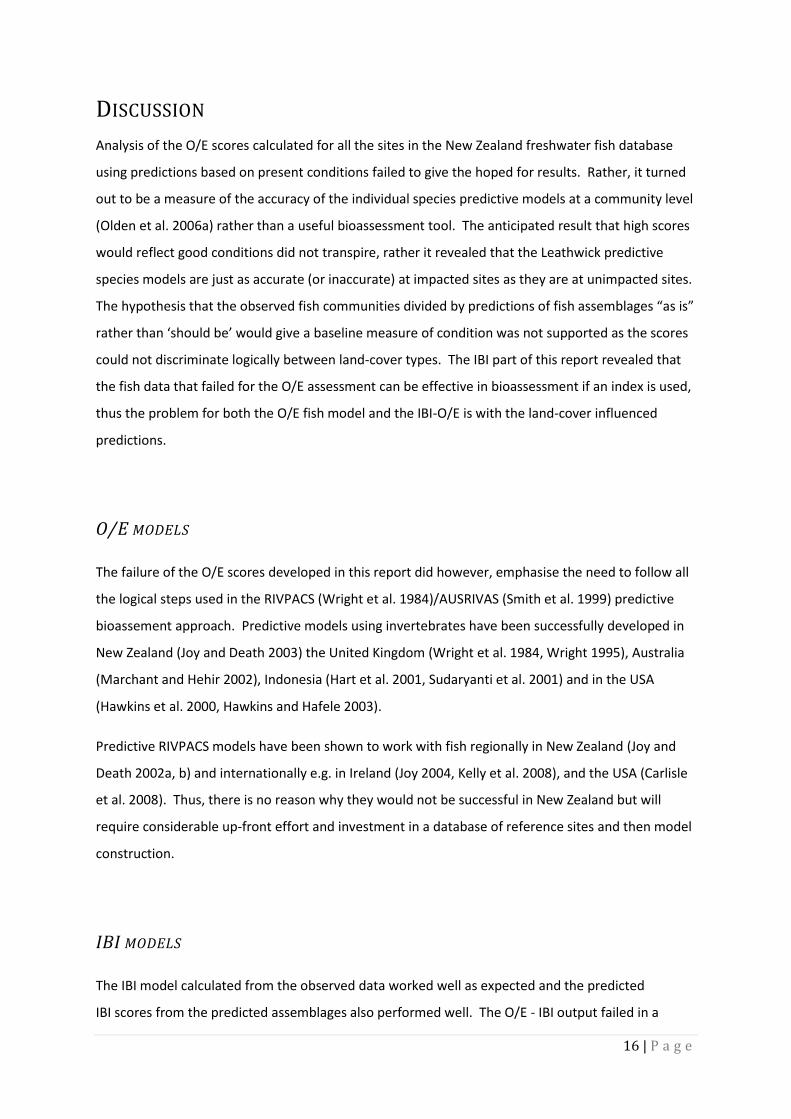
OBSERVED OVER EXPECTED IBI

The O/E - IBI scores show contradictory and incongruous scores for the REC classes (Figure 8). The

scores a virtual the reverse of the rankings from the mainly congruent observed and predicted IBI

15 | P a g e

scores above. For example the pasture sites score higher than the indigenous forest sites.

Figure 8. Average O/E - IBI score (± SE) for each REC class the predicted IBI using the best prediction threshold to maximise kappa from ROC analysis. See table 3 for details on number of sites in each class

16 | P a g e

DISCUSSION

Analysis of the O/E scores calculated for all the sites in the New Zealand freshwater fish database

using predictions based on present conditions failed to give the hoped for results. Rather, it turned

out to be a measure of the accuracy of the individual species predictive models at a community level

(Olden et al. 2006a) rather than a useful bioassessment tool. The anticipated result that high scores

would reflect good conditions did not transpire, rather it revealed that the Leathwick predictive

species models are just as accurate (or inaccurate) at impacted sites as they are at unimpacted sites.

The hypothesis that the observed fish communities divided by predictions of fish assemblages “as is”

rather than ‘should be’ would give a baseline measure of condition was not supported as the scores

could not discriminate logically between land-cover types. The IBI part of this report revealed that

the fish data that failed for the O/E assessment can be effective in bioassessment if an index is used,

thus the problem for both the O/E fish model and the IBI-O/E is with the land-cover influenced

predictions.

O/E MODELS

The failure of the O/E scores developed in this report did however, emphasise the need to follow all

the logical steps used in the RIVPACS (Wright et al. 1984)/AUSRIVAS (Smith et al. 1999) predictive

bioassement approach. Predictive models using invertebrates have been successfully developed in

New Zealand (Joy and Death 2003) the United Kingdom (Wright et al. 1984, Wright 1995), Australia

(Marchant and Hehir 2002), Indonesia (Hart et al. 2001, Sudaryanti et al. 2001) and in the USA

(Hawkins et al. 2000, Hawkins and Hafele 2003).

Predictive RIVPACS models have been shown to work with fish regionally in New Zealand (Joy and

Death 2002a, b) and internationally e.g. in Ireland (Joy 2004, Kelly et al. 2008), and the USA (Carlisle

et al. 2008). Thus, there is no reason why they would not be successful in New Zealand but will

require considerable up-front effort and investment in a database of reference sites and then model

construction.

IBI MODELS

The IBI model calculated from the observed data worked well as expected and the predicted

IBI scores from the predicted assemblages also performed well. The O/E - IBI output failed in a

17 | P a g e

similar way to the full O/E models, again it seemed to reflect the predictive ability of the

individual predictive models rather than different impacts on assemblages. The IBI analysis

was done to show that the same data that revealed a lack of usefulness of data when used as

an O/E fish assemblage score can be useful when an index approach is taken. The predictive

IBI added nothing to the analysis when using the O/E – IBI approach but would be useful for

highlighting impacted areas of the country when mapped out nationally. The IBI assessment

could be improved with the inclusion of abundance/density data and information on size

classes so that population structure could be added. The information required to improve

these models would require consistent sampling methods and protocols to achieve this and

these are now available (David et al. 2010, Joy et al. 2013).

CONCLUSIONS & RECOMMENDATIONS

Predictive O/E bioassessment models using fish have great potential to improve freshwater

ecological assessment in New Zealand. However, this study showed that taking short-cuts does not

work with these models. The model building procedure outlined in many studies worldwide shows

that initial investment in site selection and collection of reference data is crucial. This investment

may seem expensive but is a one-off and can be used for many years. The IBI approach is useful in

the absence of an O/E model, for regional and national reporting but to improve it there needs to be

upgraded to include the consistent abundance data which is now being collected now protocols are

available (David et al. 2010, Joy et al. 2013).

RECOMMENDATIONS FOR FISH AS NATIONAL INDICATORS

Freshwater fish are ideal indicators of the overall health of freshwater ecosystems as they integrate

all ecological components. At the top of food webs and influenced by both upstream and

downstream conditions fish have the greatest potential as holistic river health indicators. The tools

to enable the use of fish in national level assessment in New Zealand are available with the fish IBI

and IBI models are already being used in state of the environment reporting by many councils. The

existing fish IBI models do however, have potential for improvement with the quantitative data

collection now becoming available with the new sampling protocols (David et al. 2010, Joy et al.

2013). This new data is collected using standardised procedures and includes information on

abundance and population structure. While, the predictive modelling RIVPACs type fish models

18 | P a g e

have great potential as national indicators they require a considerable initial investment to gather

reference site data, and model building although this investment is one-off.

INDEX OF BIOTIC INTEGRITY

In the short term, the presently available IBI (Joy and Death 2004a) would be appropriate as a

national assessment indicator, however, in the long term investment in developing the IBI further to

include the newly available standardised fish data would further enhance its precision. The next

steps to develop the IBI would be to gather the fish data gathered already using the new protocols

(David et al. 2010) and any in the database that includes abundance and size details and use this

data to update the IBI. The inclusion of abundance and size class information will enhance the

precision of the IBI by including metrics encompassing abundance and size/age structure. These

new metrics have been added to an IBI developed for New Caledonia and shown to work well (Joy

and Poellabauer In Prep).

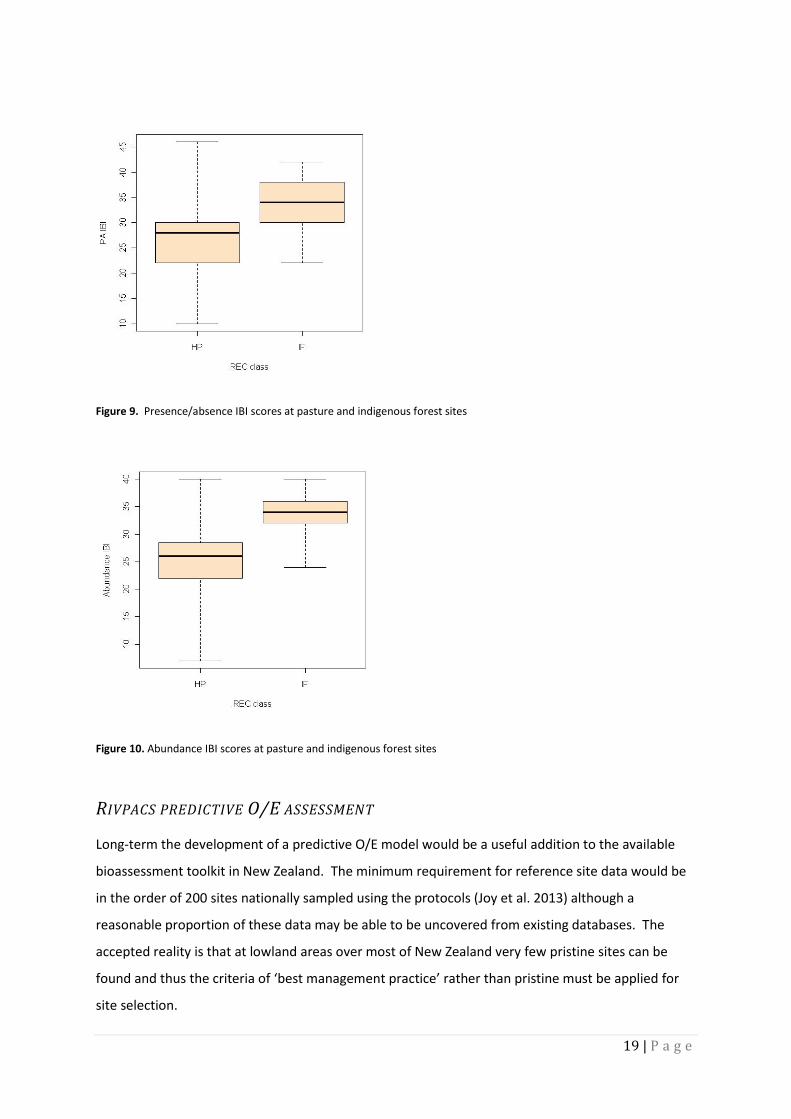
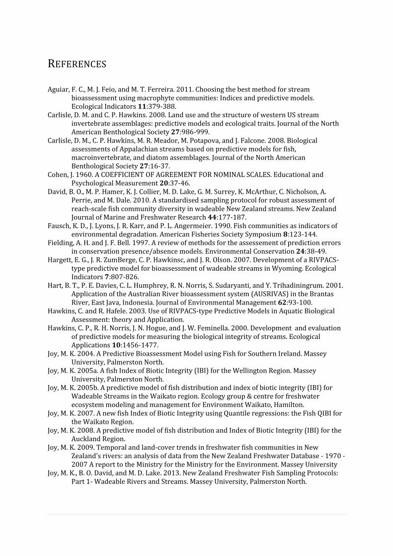
In a trail run, a sample of new data collected using the New Zealand protocols was assessed using an

upgraded IBI (with some abundance metrics added). The comparison of the presence absence and

basic abundance data and new metrics in an IBI using around 90 sites sampled using the

electrofishing protocols showed that the precision when comparing REC pasture sites with

indigenous forest sites was higher. The P value for the test for the statistic for the difference

between the average IBI scores at the two REC classes was: using presence/absence P = 0.00001457

and for the basic abundance model P = 0.00000012 . This difference can be seen in figures 9 and 10

with tighter ranges in box plots with abundance versus presence/absence IBI scores. The

comparison was limited because it was just a first attempt and didn’t include size class data, but

revealed the likelihood that there will advantages with upgrading the IBI and collecting more

comprehensive data.

19 | P a g e

Figure 9. Presence/absence IBI scores at pasture and indigenous forest sites

Figure 10. Abundance IBI scores at pasture and indigenous forest sites

RIVPACS PREDICTIVE O/E ASSESSMENT

Long-term the development of a predictive O/E model would be a useful addition to the available

bioassessment toolkit in New Zealand. The minimum requirement for reference site data would be

in the order of 200 sites nationally sampled using the protocols (Joy et al. 2013) although a

reasonable proportion of these data may be able to be uncovered from existing databases. The

accepted reality is that at lowland areas over most of New Zealand very few pristine sites can be

found and thus the criteria of ‘best management practice’ rather than pristine must be applied for

site selection.

REFERENCES

Aguiar, F. C., M. J. Feio, and M. T. Ferreira. 2011. Choosing the best method for stream bioassessment using macrophyte communities: Indices and predictive models. Ecological Indicators 11:379-388.

Carlisle, D. M. and C. P. Hawkins. 2008. Land use and the structure of western US stream invertebrate assemblages: predictive models and ecological traits. Journal of the North American Benthological Society 27:986-999.

Carlisle, D. M., C. P. Hawkins, M. R. Meador, M. Potapova, and J. Falcone. 2008. Biological assessments of Appalachian streams based on predictive models for fish, macroinvertebrate, and diatom assemblages. Journal of the North American Benthological Society 27:16-37.

Cohen, J. 1960. A COEFFICIENT OF AGREEMENT FOR NOMINAL SCALES. Educational and Psychological Measurement 20:37-46.

David, B. O., M. P. Hamer, K. J. Collier, M. D. Lake, G. M. Surrey, K. McArthur, C. Nicholson, A. Perrie, and M. Dale. 2010. A standardised sampling protocol for robust assessment of reach-scale fish community diversity in wadeable New Zealand streams. New Zealand Journal of Marine and Freshwater Research 44:177-187.

Fausch, K. D., J. Lyons, J. R. Karr, and P. L. Angermeier. 1990. Fish communities as indicators of environmental degradation. American Fisheries Society Symposium 8:123-144.

Fielding, A. H. and J. F. Bell. 1997. A review of methods for the assessement of prediction errors in conservation presence/absence models. Environmental Conservation 24:38-49.

Hargett, E. G., J. R. ZumBerge, C. P. Hawkinsc, and J. R. Olson. 2007. Development of a RIVPACS-type predictive model for bioassessment of wadeable streams in Wyoming. Ecological Indicators 7:807-826.

Hart, B. T., P. E. Davies, C. L. Humphrey, R. N. Norris, S. Sudaryanti, and Y. Trihadiningrum. 2001. Application of the Australian River bioassessment system (AUSRIVAS) in the Brantas River, East Java, Indonesia. Journal of Environmental Management 62:93-100.

Hawkins, C. and R. Hafele. 2003. Use of RIVPACS-type Predictive Models in Aquatic Biological Assessment: theory and Application.

Hawkins, C. P., R. H. Norris, J. N. Hogue, and J. W. Feminella. 2000. Development and evaluation of predictive models for measuring the biological integrity of streams. Ecological Applications 10:1456-1477.

Joy, M. K. 2004. A Predictive Bioassessment Model using Fish for Southern Ireland. Massey University, Palmerston North.

Joy, M. K. 2005a. A fish Index of Biotic Integrity (IBI) for the Wellington Region. Massey University, Palmerston North.

Joy, M. K. 2005b. A predictive model of fish distribution and index of biotic integrity (IBI) for Wadeable Streams in the Waikato region. Ecology group & centre for freshwater ecosystem modeling and management for Environment Waikato, Hamilton.

Joy, M. K. 2007. A new fish Index of Biotic Integrity using Quantile regressions: the Fish QIBI for the Waikato Region.

Joy, M. K. 2008. A predictive model of fish distribution and Index of Biotic Integrity (IBI) for the Auckland Region.

Joy, M. K. 2009. Temporal and land-cover trends in freshwater fish communities in New Zealand's rivers: an analysis of data from the New Zealand Freshwater Database - 1970 - 2007 A report to the Ministry for the Ministry for the Environment. Massey University

Joy, M. K., B. O. David, and M. D. Lake. 2013. New Zealand Freshwater Fish Sampling Protocols: Part 1- Wadeable Rivers and Streams. Massey University, Palmerston North.

21 | P a g e

Joy, M. K. and R. G. Death. 2000. Development and application of a predictive model of riverine fish community assemblages in the Taranaki region of the North Island, New Zealand. New Zealand Journal of Marine and Freshwater Research 34:241-252.

Joy, M. K. and R. G. Death. 2001. Contol of freshwater fish and crayfish community structure in Taranaki, New Zealand: dams, diadromy or habitat structure? Freshwater Biology 46:417 - 429.

Joy, M. K. and R. G. Death. 2002a. A discriminant analysis investigation of reference site fish assemblages in the Manawatu-Wanganui region, North Island, New Zealand. Pages 319-322 in R. G. Wetzel, editor. International Association of Theoretical and Applied Limnology, Vol 28, Pt 1, Proceedings. E Schweizerbart'sche Verlagsbuchhandlung, Stuttgart.

Joy, M. K. and R. G. Death. 2002b. Predictive modelling of freshwater fish as a biomonitoring tool in New Zealand. Freshwater Biology 47:2261-2275.

Joy, M. K. and R. G. Death. 2003. Biological assessment of rivers in the Manawatu-Wanganui region of New Zealand using a predictive macroinvertebrate model. New Zealand Journal of Marine and Freshwater Research 37:367-379.

Joy, M. K. and R. G. Death. 2004a. Application of the index of biotic integrity methodology to New Zealand freshwater fish communities. Environmental Management 34:415-428.

Joy, M. K. and R. G. Death. 2004b. Predictive modelling and spatial mapping of freshwater fish and decapod assemblages using GIS and neural networks. Freshwater Biology 49:1036-1052.

Joy, M. K., I. M. Henderson, and R. G. Death. 2000. Diadromy and longitudinal patterns of upstream penetration of freshwater fish in Taranaki, New Zealand. New Zealand Journal of Marine and Freshwater Research 34:531-543.

Joy, M. K. and C. Poellabauer. In Prep. A freshwater fish index of biotic integrity for New Caledonia. Environmental Management.

Karr, J. R. 1981. Assessments of biotic integrity using fish communities. Fisheries 6:21-27. Karr, J. R. 1991a. Biological integrity: a long neglected aspect of water resource management.

Ecological Applications 1:66-84. Karr, J. R. 1991b. Ecological integrity: Protecting earths life support systems.in R. Costanza, B. G.

Norton, and B. D. Haskell, editors. Ecosystem Health: Goals for Environmental Management. Island Press, California.

Karr, J. R., K. D. Fausch, P. L. Angermeier, P. R. Yant, and I. J. Schlosser. 1986. Assessing biological integrity in running waters: A method and its rationale. Illinois Natural History Survey Special Publication, Champaign, Illinois.

Kelly, F., T. Champ, M. Neasa, Mary Kelly-Quinn, Simon Harrison, Alison Arbuthnott, Paul Giller, Mike Joy, Kieran McCarthy, Paula Cullen, Chris Harrod, Phil Jordan, D. Griffiins, and R. Rosell. 2008. Investigation of the Relationship between Fish Stocks, Ecological Quality Ratings (Q-Values), Environmental Factors and Degree of Eutrophication.

Kennard, M. J., B. D. Harch, B. J. Pusey, and A. H. Arthington. 2006. Accurately defining the reference condition for summary biotic metrics: A comparison of four approaches. Hydrobiologia 572:151-170.

Leathwick, D. M., K. Julian, J. Elith, and D. Rowe. 2008a. Predicting the distributions of freshwater fish species for all New Zealands rivers and streams. NIWA, Hamilton.

Leathwick, J. R., K. Julian, J. Elith, and D. Rowe. 2008b. Predicting the distribution of freshwater fish species for all New Zealand's rivers and streams. NIWA Client Report HAM2008-005, National Institute of Water and Atmospheric Research LtD.

Marchant, R. and G. Hehir. 2002. The use of AUSRIVAS predictive models to assess the response of lotic macroinvertebrates to dams in south-east Australia. Freshwater Biology 47:1033-1050.

McCormick, F. H., D. V. Peck, and D. P. Larsen. 2000. Comparison of geographic classification schemes for mid-Atlantic stream fish assemblages. Journal of the North American Benthological Society 19:385-404.

22 | P a g e

McDowall, R. M. 1988. Diadromy in fishes: migrations between marine and freshwater environments. Croom Helm, London.

McDowall, R. M. 1990. New Zealand Freshwater Fishes: A Natural History and Guide. Heinemann Reed, Auckland.

McDowall, R. M. and J. Richardson. 1983. The New Zealand freshwater fish database-a guide to input and output. Fisheries Research Division Information leaflet 12, Ministry of agriculture and Fisheries, Wellington.

McDowall, R. M. and M. J. Taylor. 2000. Environmental indicators of habitat quality in a migratory freshwater fish fauna. Environmental Management 25:357-374.

Olden, J. D., M. K. Joy, and R. G. Death. 2006a. Rediscovering the species in community-wide predictive modeling. Ecological Applications 16:1449-1460.

Olden, J. D., M. K. Joy, and R. G. Death. 2006b. Rediscovering the species in community-wide predictive modeling. Ecological Applications 16.

Richardson, J. 1989. The all-new freshwater fish database. Freshwater catch 41:20-21. Richardson, J. 1993. Database tops 10 000 records. Water & Atmoshpere 1:14-15. Robertson, D. M., D. A. Saad, and D. M. Heisey. 2006. A regional classification scheme for

estimating reference water quality in streams using land-use-adjusted spatial regression-tree analysis. Environmental Management 37:209-229.

Simpson, J. and R. H. Norris. 2000. Biological assessment of water quality: development of AUSRIVAS models and outputs. Pages 125-142 in J. F. Wright, D. W. Sutcliffe, and M. T. Furse, editors. Assessing the biological quality of freshwaters. RIVPACS and other techniques. Freshwater Biological Association, Ambleside, UK.

Smith, M. J., W. R. Kay, D. H. D. Edward, P. J. Papas, K. S. J. Richardson, J. C. Simpson, A. M. Pinder, D. J. Cale, P. H. J. Horwitz, J. A. Davis, F. H. Yung, R. H. Norris, and S. A. Halse. 1999. AusRivAS: using macroinvertebrates to assess ecological condition of rivers in Western Australia. Freshwater Biology 41:269-282.

Snelder, T. and B. J. F. Biggs. 2002. Multi-Scale River Environment Classification for Water Resources Management. Journal of the American Water Resources Association 38:1225-1240.

Snelder, T., B. J. F. Biggs, M. Weatherhead, and K. Niven. 2002. A brief overview of New Zealands River Environment Classification. NIWA, Christchurch.

Snelder, T., F. Cattaneo, A. M. Suren, and B. J. F. Biggs. 2004. Is the River Environment Classification an improved landscape-scale classification of rivers? Journal of the North American Benthological Society 23:580-598.

Snelder, T. and P. Guest. 2000. The ‘river ecosystem management framework’ and the use of river environment classification as a tool for planning. NIWA Client Report: CHC00/81, Ministry for the Environment National Institute of Water & Atmospheric Research Ltd.

Sudaryanti, S., Y. Trihadiningrum, B. T. Hart, P. E. Davies, C. Humphrey, R. H. Norris, J. Simpson, and L. Thurtell. 2001. Assessment of the biological health of the Brantas River, East Java, Indonesia using the Australian River Assessment System (AUSRIVAS) methodology. Aquatic Ecology 35:135-146.

Tsang, Y. P., G. K. Felton, G. E. Moglen, and M. Paul. 2011. Region of influence method improves macroinvertebrate predictive models in Maryland. Ecological Modelling 222:3473-3485.

Wang, L., T. Brenden, P. Seelbach, A. Cooper, D. Allan, R. J. Clarck, and M. Wiley. 2008. Landscape based identification of human disturbance gradents and reference conditions for michian streams. environ Monit Assess 141.

Wright, J. F. 1995. Development and use of a system for predicting the macroinvertebrate fauna in flowing waters. Australian Journal of Ecology 20:181-197.

Wright, J. F., D. Moss, P. D. Armitage, and M. T. Furse. 1984. A preliminary classification of running water-sites in Great Britian based on macro-invertebrate species and the prediction of community type using environmental data. Freshwater Biology 14:221-256.

23 | P a g e

Yuan, L. L., C. P. Hawkins, and J. Van Sickle. 2008. Effects of regionalization decisions on an O/E index for the US national assessment. Journal of the North American Benthological Society 27:892-905.