OPEN ACCESS

Fresnel coherent diffractive imaging: treatmentand analysis of dataTo cite this article: G J Williams et al 2010 New J. Phys. 12 035020

 

View the article online for updates and enhancements.

You may also likeFlow-Electrode Capacitive Deionization(FCDI) Using Suspensions of 2D MaterialsAs ElectrodesAranzazu Carmona Orbezo and RobertAW Dryfe

-

XPM-induced modulation instability insilicon-on-insulator nano-waveguides andthe impact of nonlinear lossesDeepa Chaturvedi, Ajit Kumar andAkhilesh Kumar Mishra

-

Fresnel coherent diffractive imagingtomography of whole cells in capillariesMac B Luu, Grant A van Riessen, BrianAbbey et al.

-

This content was downloaded from IP address 103.117.108.37 on 13/02/2022 at 05:12

T h e o p e n – a c c e s s j o u r n a l f o r p h y s i c s

New Journal of Physics

Fresnel coherent diffractive imaging: treatmentand analysis of data

G J Williams1,3,4,5, H M Quiney1,3, A G Peele2,3 and K A Nugent1,3

1 School of Physics, The University of Melbourne, Melbourne, VIC, Australia2 Department of Physics, La Trobe University, Bundoora, VIC, Australia3 Australian Research Council Centre of Excellence for Coherent X-rayScience, School of Physics, The University of Melbourne, Melbourne, VIC,AustraliaE-mail: gjwillms@slac.stanford.edu

New Journal of Physics 12 (2010) 035020 (18pp)Received 28 November 2009Published 31 March 2010Online at http://www.njp.org/doi:10.1088/1367-2630/12/3/035020

Abstract. Fresnel coherent diffractive imaging (FCDI) is a relatively recentaddition to the suite of imaging tools available at third generation x-ray sources.It shares the strengths of other coherent diffractive techniques: resolutionlimits that are independent of focusing optics, single-plane measurementand high dose efficiency. The more challenging experimental geometryand detailed reconstruction algorithms of FCDI provide enhanced numericalstability and convergence properties to the iterative algorithms commonly used.Experimentally, a diverging beam is utilized, which facilitates sample alignmentand allows the imaging of extended samples. We describe the underlyingphysics and assumptions that give rise to the FCDI iterative reconstructionalgorithms, as well as their implications for the design of a successful FCDIexperiment.

4 Current address: SLAC National Accelerator Laboratory, Menlo Park, CA, USA.5 Author to whom any correspondence should be addressed.

New Journal of Physics 12 (2010) 0350201367-2630/10/035020+18$30.00 © IOP Publishing Ltd and Deutsche Physikalische Gesellschaft

2

Contents

1. Introduction 22. Theory 3

2.1. Propagation of light and the origin of the ESW . . . . . . . . . . . . . . . . . 32.2. Algorithms . . . . . . . . . . . . . . . . . . . . . . . . . . . . . . . . . . . . 4

3. Experiment 63.1. Important criteria . . . . . . . . . . . . . . . . . . . . . . . . . . . . . . . . . 63.2. Stability . . . . . . . . . . . . . . . . . . . . . . . . . . . . . . . . . . . . . . 73.3. Equipment . . . . . . . . . . . . . . . . . . . . . . . . . . . . . . . . . . . . . 8

4. Result 94.1. Properties of the white-field data . . . . . . . . . . . . . . . . . . . . . . . . . 94.2. Properties of the ESW data . . . . . . . . . . . . . . . . . . . . . . . . . . . . 10

5. Discussion 115.1. Data handling . . . . . . . . . . . . . . . . . . . . . . . . . . . . . . . . . . . 115.2. Beam recovery . . . . . . . . . . . . . . . . . . . . . . . . . . . . . . . . . . 135.3. ESW recovery . . . . . . . . . . . . . . . . . . . . . . . . . . . . . . . . . . . 14

6. Conclusion 16Acknowledgments 17References 17

1. Introduction

Coherent diffractive imaging (CDI) is a method whereby one plane of diffraction data maybe transformed into an image of the sample. The practical limit to the resolution of imagesso acquired is based on the numerical aperture—the highest angle at which scattered probeparticles can be measured—of the detector, not on the image-forming lens. This is generallyachieved by an iterative algorithm that forces the wave leaving the object to be mutuallyconsistent with its diffraction pattern and the experimenter’s knowledge of the sample.

The method was first demonstrated by Miao et al [1] on an Au test object and hassince been applied to a wide range of samples, including biological materials [2]–[5] andfoams [6]. While these demonstrations have used plane-wave illumination in a forward-scattering geometry, the method is not limited in this way; it has also been implemented ina Bragg-angle geometry [7]–[9], in a scanning-mode geometry [10], with partially coherentillumination [11] and with phase structure in the illumination of the sample [12]. The focus ofthis paper will be on the application of the described technique in the last case: Fresnel CDI(FCDI).

FCDI has a number of intriguing properties. Firstly, it can be shown that, in the absence ofnoise, there exists only one solution [13] to the FCDI problem. This is in contrast to the plane-wave case, where there is a translational invariance of the sample underlying the emergenceof the far-field diffraction pattern. Practically, this means that the ambiguities identified byBates [14] are not present and that—even in the presence of noise—iterative algorithmsconverge quickly and consistently. Secondly, when implemented as a finite, diverging beamilluminating a sample, the only region of a large sample contributing to the far-field intensityfalls within the beam. This means that a region of interest on a large sample can be easily

New Journal of Physics 12 (2010) 035020 (http://www.njp.org/)

3

accessed [15, 16]. Finally, in certain instances, it is possible to derive quantitative informationabout the thickness [17] of the sample from the recovered ‘exit surface wave’ (ESW).

In this paper, we aim to explain the concepts underlying the FCDI approach and give adetailed account of the data treatment procedures used in and an interpretation of the resultsin [12].

2. Theory

2.1. Propagation of light and the origin of the ESW

An explicit manipulation of the wave leaving the sample lies at the heart of FCDI. Whereas,in plane-wave CDI, it is often sufficient to use only the Fourier transform, F̂, to propagatebetween the sample and detector planes, the phase structure introduced into the illuminatingwave requires a more careful treatment of this quantity in FCDI. We consider the paraxialpropagation of a monochromatic wave of wavelength λ, ψ(rn, zn), contained in a plane at zn tosome other plane at zm to be defined by [18]

ψ(rm, zm)=−i

λznmexp

(i2π znm

λ

)exp

(iπr 2

m

λznm

)×

∫drnψ (rn, zn) exp

(iπr 2

n

λznm

)exp

(−2π irn · rm

λznm

)=2(rm, znm)× F̂ [4(rn, znm) ψ (rn, zn)], (1)

where, in the final line, we have introduced the functions 2(rn, znm) and 4(rn, znm) containingthe prefactors to the integral and the spherical phase term in the integrand, respectively, andrecognizing that this integral can be expressed as a Fourier transform. Henceforth, the sampleplane will be indicated with s, the detector plane with d and the focal plane with f, e.g. zfd

denotes the focus-to-detector distance. We note that the primary departure of the propagationin FCDI to that of plane-wave CDI is that in the latter 4(rd, zsd)= 1, as zsd = ∞ is normallyassumed.

The physical quantity of interest in FCDI is the transmission function of the sample. In thecase of thin, singly scattering objects, the projection approximation [19] holds, i.e. the thickness,τ(r), of the sample must obey the following relation with respect to the desired resolution δ andthe wavelength

τ(r)�2

kθ 2max

(2)

�4δ2

πλ, (3)

where θmax is the largest angle to which significant scattering is measured and assumed to besmall. For a two-dimensional (2D) measurement, we recognize that the physical ESW leavingan object is related to the incident wave ψ(r, zn) and the object’s 3D refractive index map,n(r, z), projected onto an exit plane by ψESW(r, zs)= T(r s)ψ(r s, zs), where

T(r)= exp

[i2π

λ

∫sample

dz n(r, z)

]' exp

{i2π

λ[1 − δ(r)+ iβ(r)]τ(r)

}. (4)

New Journal of Physics 12 (2010) 035020 (http://www.njp.org/)

4

These three approximations—paraxiality, single scattering and projection—are normallycomfortably accommodated by x-ray FCDI experiments.

In FCDI, neglecting intensity variations in the pupil function, one introduces a waveof the form ψ(r s, zs)≈ exp

(−iπr 2

s /λzfs

)to the sample. In the case where this is exactly

true, the input of the propagation operator in equation (1) becomes 4(r s, z′

sd

)T (r s), where

(z′

sd)−1

= z−1fd − z−1

fs is the difference in the reciprocals of the focus-to-detector and focus-to-sample distances. This important realization allows the use of fast Fourier transform (FFT) inthe implementation of the algorithm of section 2.2.2.

2.2. Algorithms

Generally speaking, the goal of CDI is to recover the complete complex wave that has givenrise to a measured diffraction pattern in order to arrive at an image of the sample, whichis a manifestation of n(r, z) or its projection. This is usually accomplished by means of aniterative process, which propagates the trial wave—called the ‘iterate’—between the sample anddetector planes. In each plane, the iterate is constrained to display any properties of the objectthat may be known a priori. The most obvious constraint is that the square modulus of theiterate in the detector plane must match the measured intensity distribution. This is commonlycalled a ‘modulus’ constraint [20]. We call the result of applying the modulus constraint to aniterate as the current ‘estimate’ of the wave. Due to the sampling requirement on the intensitydistribution, the sample—or the portion of the sample contributing to the diffraction—must befinite in extent. This gives rise to the commonly applied ‘support’ constraint in the sample plane.Numerous additional constraints have been suggested; however, we will here restrict ourselvesto these two.

The iterative algorithms common in CDI can be compactly expressed in a projectornotation [21, 22], where an iterate, ρk , is regarded as a vector in an N -dimensional vectorspace. The task of enforcing the constraints is assigned to projection operators, e.g. we callthe modulus constraint πm and the support constraint πs. For simplicity, these operators actexplicitly in the sample plane, so that the propagation must be built into the modulus constraint:πm = F−1π̃mF, where the tilde indicates the projector as operating in the Fourier space. We willobey the following convention: ρk is the iterate and πmρk is the estimate of the target wave onthe kth iteration.

Using this notation, we can state the algorithms most commonly used in FCDI. The kthiterate subjected to error reduction (ER) [20, 23] is

ρk+1 = (πsπm) ρk, (5)

while for hybrid input/output (HIO) [23],

ρk+1 = [1 + (1 +β)πsπm −πs −βπm] ρk, (6)

where β is the familiar, scalar HIO parameter. The experimental demonstration presented insections 4 and 5 was achieved using only ER and a support constraint that was successivelyupdated, similar to the shrinkwrap algorithm of Marchesini et al [24].

The support generated here was generated by a two-step method: (i) find all regions withinthe recovered wave that have magnitude above a certain value and assign these to be unity inthe support array; and (ii) convolve the support array with a Gaussian function of narrow width.The operation πs is then accomplished by multiplying this array by the estimate.

New Journal of Physics 12 (2010) 035020 (http://www.njp.org/)

5

2.2.1. The beam recovery algorithm. The wave illuminating the object must be known in orderto correctly separate its features from those of the sample’s ESW. We achieve this by meansof the algorithm demonstrated in Quiney et al [25]. This algorithm requires that one make ameasurement of the far-field intensity arising from a lens and know the size of the pupil functionof the lens the focal length of the lens, and the focal-plane-to-detector distance.

With this information in hand, we can iteratively recover the phase of the divergingbeam in the plane of the detector, which can, of course, be propagated to any other planenumerically. This procedure requires propagation between three planes, each perpendicular tothe propagation direction: the lens plane, zl; the focal plane, zf; and the detector plane, zd.Unfortunately, the propagator in the zd- and zl-planes oscillates too quickly to be properlysampled in the discrete array. This is overcome by recognizing that the wave is formed throughthe multiplication of a slowly varying component with a quickly varying one. By analyticallypropagating the quickly varying component and numerically propagating the other, the iterativealgorithm retains its phase-retrieval properties and remains numerically stable.

Let the wave in the lens plane be ψ(r l, zl)= P(r l) exp(iπr 2

l /λzlf

), where P(r l) is

the complex pupil function of the lens and zlf is its focal length. Similarly, ψ(rd, zd)=

P̃(rd) exp(−iπr 2

d/λzfd

)is the wave in the detector plane. The steps in the algorithm are

1. Propagate from zl to zf: ψk(r f, zf)=2(r f, zlf)F̂ [Pk(r l)]

2. Propagate from zf to zd: P̃k(rd)= −i exp (i2π zfd/λ) F̂ [ψk(r f, zf)4(r f, zfd)]

3. Apply modulus constraint: P̃ ′

k(rd)= P̃exp(rd)×P̃k(rd)

|P̃k(rd)|

4. Propagate from zd to zf: ψ ′

k(r f, zf)=2(r f, zdf)F̂[

P̃ ′

k(rd)]

5. Propagate from zf to zl: P ′

k(r l)= −i exp (i2π zfl/λ) F̂ [ψk(r f, zf)4(r f, zfl)]

6. Enforce support constraint on pupil: Pk+1(r l)= πs P ′

k(r l)

7. Use Pk+1(r l) in 1

Once convergence has been obtained, the algorithm is halted at step 2, which constitutes thebest estimate of the pupil function in the detector plane. The estimate of the wave in the detectorplane on the N th iteration is ψ(rd, zd)= P̃N (rd) exp

(−iπr 2

d/λzfd

).

To establish a connection to the operator notation, we introduce projectors for the variousmultiplications in the algorithm: π nm

2 for the multiplication by2(rm, znm) in step 1, π nm4 for that

by 4(rm, znm) and πnmp for that by −iexp(i2π znm/λ). The (k + 1)th iterate is then

Pk+1 =

[πsπ

flp F̂ π

fl4 π

df2 F̂ π̃m π

fdp F̂ π

fd4 π

lf2 F̂

]Pk. (7)

2.2.2. The ESW recovery algorithm. While one might be tempted to simply include apropagation to the sample plane in the algorithm of section 2.2.1, one must remember thatP(r l) is constrained to be slowly varying, which cannot be assumed in the case of the finalestimate of the sample’s ESW. Therefore, it becomes necessary to implement the algorithm intwo parts: first recover the phase of the incident illumination and then recover the phase of thesample’s diffraction. As described at the end of section 2.1, a ‘curvature component’ must bereintroduced into the output of the beam recovery algorithm before using it in the recovering ofthe ESW.

New Journal of Physics 12 (2010) 035020 (http://www.njp.org/)

6

The algorithm for recovering the ESW itself was described by Williams et al [12]. Thereare a few key differences between the Fresnel and plane-wave variants of CDI. Among these isthe question of how the incident beam is treated in each case. In plane-wave CDI, the sampleis small compared to the extent of the beam, but since the interference between the beam andlight scattered by the sample is occluded by a beam stop—which protects the detector from theundiffracted beam—a transmission function can be easily recovered using Babinet’s principle,i.e. for regions sufficiently far away from the origin, F̂[ f (r)] = F̂[1 − f (r)]. By contrast, inFCDI, we measure the intensity arising from T(r s)ψ(r s, zs) propagated to the detector plane.An important consideration is that while the beam may be used to define a region of interestin the sample [15, 16], the only requirement is that the object be illuminated with sufficientphase curvature [26]. In other words, the beam may be so large in the plane of the sample that anumerical propagation back to that plane will result in the overfilling of that unit of the discreteFourier space.

A further consideration concerns the ability to impose the support constraint. In principle,one wishes to apply this to the transmission function; however, this requires a division operationin the plane of the sample. In the early stages of the reconstruction, this can prove to be quiteunstable numerically, as many regions of the illumination may approach zero magnitude. Toaddress these concerns, it is useful to perform a subtraction of the known illuminating wavefrom the iterate of the far-field ESW. In essence, this means that the quantity dealt with in theiterative scheme is [T(r s)− 1]ψ(r s, zs). To account for this subtraction in the context of ER andHIO, we introduce a new projection operator: π̃WF. The modified algorithm is then

ρk+1 = πsπmρk = πsF̂−1π̃−1

WFπ̃mπ̃WFF̂ρk. (8)

3. Experiment

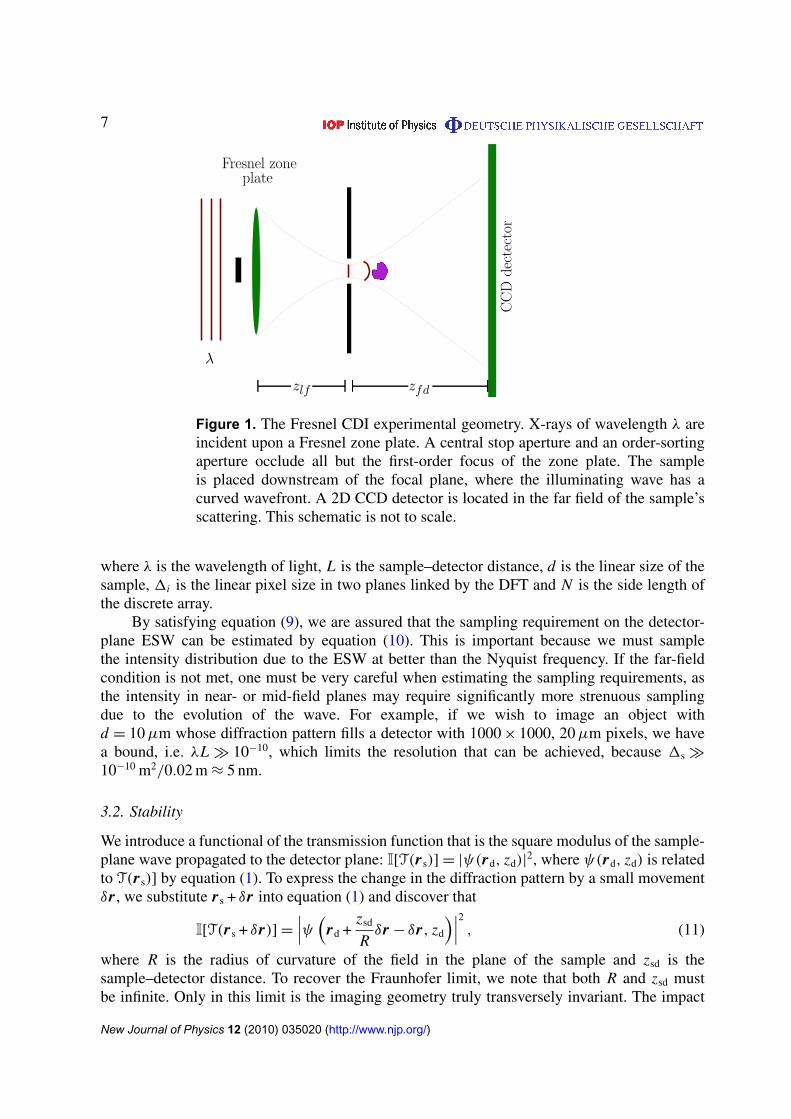
The Fresnel CDI experimental geometry used here is superficially very similar to that of ascanning x-ray microscope, as can be seen in figure 1. There are three notable differences: theorder-sorting aperture of the zone plate was placed in the focal plane and made as small aspossible, the sample was displaced to some defocus distance where significant curvature hasdeveloped in the illuminating field emerging from the focus, and a 2D integrating detector wasused. In this section, we describe the rationale for choosing the stated experimental parametersand detail the data collection.

3.1. Important criteria

We introduce two useful heuristics that have a strong influence on FCDI experiment design, thefar-field condition

1 �d2

λL(9)

and the discrete Fourier transform (DFT) relation for pixel size in the sample and detectorplanes

1s =λL

N1d, (10)

New Journal of Physics 12 (2010) 035020 (http://www.njp.org/)

7

z dfz fl

λ

enozlenserFetalp

CCDdectector

Figure 1. The Fresnel CDI experimental geometry. X-rays of wavelength λ areincident upon a Fresnel zone plate. A central stop aperture and an order-sortingaperture occlude all but the first-order focus of the zone plate. The sampleis placed downstream of the focal plane, where the illuminating wave has acurved wavefront. A 2D CCD detector is located in the far field of the sample’sscattering. This schematic is not to scale.

where λ is the wavelength of light, L is the sample–detector distance, d is the linear size of thesample, 1i is the linear pixel size in two planes linked by the DFT and N is the side length ofthe discrete array.

By satisfying equation (9), we are assured that the sampling requirement on the detector-plane ESW can be estimated by equation (10). This is important because we must samplethe intensity distribution due to the ESW at better than the Nyquist frequency. If the far-fieldcondition is not met, one must be very careful when estimating the sampling requirements, asthe intensity in near- or mid-field planes may require significantly more strenuous samplingdue to the evolution of the wave. For example, if we wish to image an object withd = 10µm whose diffraction pattern fills a detector with 1000 × 1000, 20µm pixels, we havea bound, i.e. λL � 10−10, which limits the resolution that can be achieved, because 1s �

10−10 m2/0.02 m ≈ 5 nm.

3.2. Stability

We introduce a functional of the transmission function that is the square modulus of the sample-plane wave propagated to the detector plane: I[T(r s)] = |ψ(rd, zd)|

2, where ψ(rd, zd) is relatedto T(r s)] by equation (1). To express the change in the diffraction pattern by a small movementδr , we substitute r s + δr into equation (1) and discover that

I[T(r s + δr)] =

∣∣∣ψ (rd +

zsd

Rδr − δr, zd

)∣∣∣2, (11)

where R is the radius of curvature of the field in the plane of the sample and zsd is thesample–detector distance. To recover the Fraunhofer limit, we note that both R and zsd mustbe infinite. Only in this limit is the imaging geometry truly transversely invariant. The impact

New Journal of Physics 12 (2010) 035020 (http://www.njp.org/)

8

upon CDI is immediately obvious: the effect of a moving sample is to ‘blur’ the diffractionpattern in the detector plane with a scaling parameter that goes as the magnification of theimaging system.

In FCDI, this poses a serious problem. As a consequence of the requirement that thebeam at the sample have a Fresnel number that is greater than 5 [26], the magnification factorsfor these experiments are typically 500–1000. Pragmatically, the sample stability requirementreduces to a question of how much blurring of the diffraction pattern can be tolerated in theiterative scheme or compensated for after-the-fact. As a heuristic, one might require that theblurring due to motion be much less than the point spread function of the CCD, which istypically 20µm or more. The geometry of the experiment described here, which ultimatelygives a resolution 24 nm, provides a bound:

δr �

( zsd

R− 1

)× 20µm �

(0.5 m

1.0 mm− 1

)× 20µm � 40 nm. (12)

Although this is quite a stringent requirement, we note that it is not directly dependent upon theresolution of any image derived from the final reconstruction of the ESW.

Equation (11) applies equally to plane-wave CDI. In order for the experimental geometryto be transversely invariant, zsd/R ' 1 and zsd must satisfy the far-field condition given byequation (9). These two conditions are probably not met in many plane-wave CDI experiments,but equation (12) indicates that sample motion would become problematic only as its magnitudeapproaches the point spread function of the detector.

3.3. Equipment

The iterative algorithms used in CDI typically depend upon the coherent propagation oflight, as described in section 2. As a result, most such experiments are conducted at third-generation x-ray sources. The experiment described here was conducted at the Advanced PhotonSource on beamline 2-ID-B [27], which provided 1.8 keV photons using a spherical gratingmonochromator. In this beamline geometry, the monochromator’s exit slit may be closed toimprove the transverse coherence of the beam. This highly coherent, quasi-monochromaticbeam exits the transport pipe by traversing a 200 nm thick, 700µm2 Si3N4 window. This windowis approximately 8 m from the exit slit.

A Fresnel zone plate was used to create the diverging beam required by FCDI. In thiscase, the zone plate had diameter 160µm and an outermost-zone radius of 50 nm—which, inconjunction with a 20µm central stop and 15µm order-sorting aperture, gave rise to a divergingbeam of sufficient quality to be used in this experiment. An identical Si3N4 window was usedon the detector’s evacuated flight path. By placing the window very close to the sample, itsscattering was minimally affected by absorption or rescattering, while the total air path seen bythe beam was limited to about 1.5 cm. The detector used for this experiment was a PrincetonInstruments direct-read CCD with 24µm, square pixels in an array of 1340 × 1300. The CCDwas thermoelectrically cooled against a liquid N2 bath to −50 ◦C. With a sample of largestdimension 8µm and the detector 0.6 m from the sample plane, the conditions described byequations (9) and (10) were met.

The data were collected using CCDImageServer software developed at the APS. Theprogram can be configured to poll and record any process variables available to the EPICS-based control system. This facilitates the later analysis and troubleshooting of any inconsistentdata.

New Journal of Physics 12 (2010) 035020 (http://www.njp.org/)

9

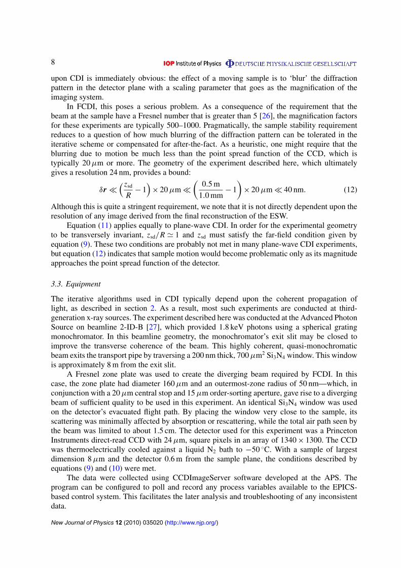
Figure 2. The reconstructed illuminating x-ray wave. (a) An image of thefar-field intensity at the detector due to the first order of the zone plate;(b) the recovered magnitude of this wave in the sample plane. Note that inthe sample plane the illumination does not ‘fit’ within the discrete array of thereconstruction. This poses no real difficulty in FCDI so long as the sample’scontribution to the far-field intensity is properly sampled. The scaling used indisplay is linear.

The sample used for this experiment was seven nested chevrons patterned in Au bylithography. One of the chevrons had side length of approximately 8µm, while the others werecontained in a square with ∼1µm side length. The Au was approximately 150 nm thick andsupported on a thick Si3N4 membrane.

4. Result

Broadly, two types of measurement are required. The ‘white-field’ data are collected withouta sample in the path of the beam and are used to recover the complex illuminating wave. The‘ESW’ data are collected when the sample is placed in the x-ray beam and are used in theiterative scheme in conjunction with the recovered complex illumination to phase the ESW inthe detector.

4.1. Properties of the white-field data

These data are normally taken at intervals throughout the longer sample measurement, so thata change in the illumination does not unduly interfere with data analysis. Figure 2(a) shows atypical far-field ‘doughnut’ arising from the first-order focus of a zone plate. We note that thisis essentially a low-resolution image of the pupil function, complete with the shadow due to thecentral stop. The only scattering outside this donut is due to the order-sorting aperture or theair path, i.e. we expect no features smaller than the diffraction-limited spot of the zone plate tobe present in the reconstruction. This is a reflection of the near-ideal, thin-lens behavior of theoptical configuration.

New Journal of Physics 12 (2010) 035020 (http://www.njp.org/)

10

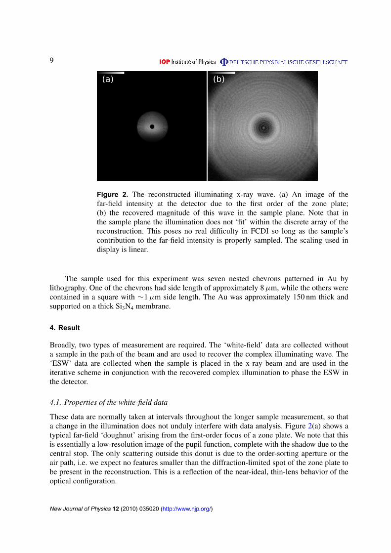
Figure 3. The treated FCDI data used in this experiment. The central regionof the data contains the interference between the illuminating wave and thesample’s ESW. It is here that we can see a ‘shadow image’ of that region ofthe sample that is illuminated. The scattering outside this region is due to thesample’s ESW alone. The dark bands along the top and the right-hand side areregions where the intensity was not measured. No constraint is placed on thereconstructed wave in these regions. (a) The data used for the lower qualityreconstruction (R > 0.9957); (b) represents an exposure that is a factor of 3shorter (R > 0.9959). The logarithm of the square root of the measured intensityis displayed.

4.2. Properties of the ESW data

Examining figure 3(a), there are two obvious differences from the white-field data of figure 2(a).First, a ‘shadow’ of the sample appears inside the beam due to the zone plate. If one wereto truncate the data at the edge of the beam, this would form an in-line-holography data set.Experimentally, the shadow is quite useful, as it allows one to place the sample in a preferredregion of the illumination. For example, it is normally wise to avoid placing an interestingregion of the sample on the optical axis, as the illuminating wave is changing quite rapidly andits reconstruction tends to work less well there. As we will describe in section 5.1, this shadowimage provides direct input on the motion of the sample over time. Figure 3(a) shows the treatedintensity used for the lower quality reconstruction, whereas figure 3(b) shows the intensity usedfor the highest quality reconstruction.

The second notable departure is the presence of strong x-ray scattering at high angles.This is the primary indication that the reconstructed ESW will yield high-resolution sampleinformation. A close examination of the fringes at high angle will also reveal how well sampledthe diffraction pattern is and give an estimate of the visibility, which is a critical indicator ofwhether the illuminating wave is sufficiently coherent to be accurately propagated by the methodin section 2.

It is useful to perform a ‘magnification check’ immediately after positioning the samplein the illumination. This allows the sample–focal plane distance to be measured under theassumptions of geometrical optics. This is accomplished by collecting one frame of data,moving a motor perpendicular to the beam by a known amount—for example, 1µm—andacquiring one more frame. The motion of the shadow image in the detector plane in microns

New Journal of Physics 12 (2010) 035020 (http://www.njp.org/)

11

689.0

889.0

99.0

299.0

499.0

699.0

899.0

1

0 0001 0002 0003 0004 0005 0006

Cro

ss-c

orre

latio

n co

effic

ient

Time (s)

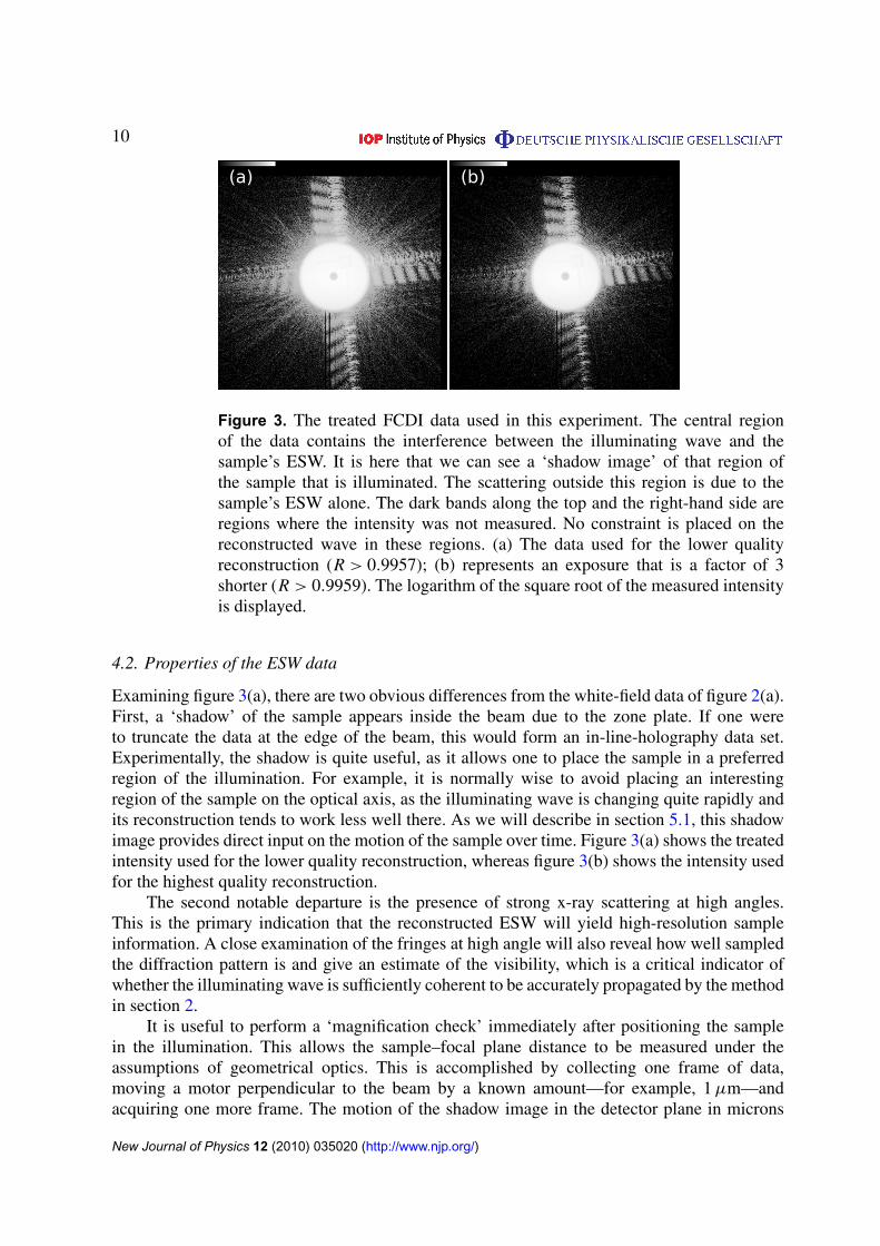
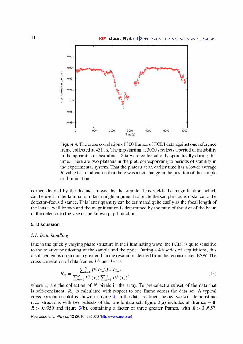
Figure 4. The cross correlation of 800 frames of FCDI data against one referenceframe collected at 4311 s. The gap starting at 3000 s reflects a period of instabilityin the apparatus or beamline. Data were collected only sporadically during thistime. There are two plateaus in the plot, corresponding to periods of stability inthe experimental system. That the plateau at an earlier time has a lower averageR-value is an indication that there was a net change in the position of the sampleor illumination.

is then divided by the distance moved by the sample. This yields the magnification, whichcan be used in the familiar similar-triangle argument to relate the sample–focus distance to thedetector–focus distance. This latter quantity can be estimated quite easily as the focal length ofthe lens is well known and the magnification is determined by the ratio of the size of the beamin the detector to the size of the known pupil function.

5. Discussion

5.1. Data handling

Due to the quickly varying phase structure in the illuminating wave, the FCDI is quite sensitiveto the relative positioning of the sample and the optic. During a 4 h series of acquisitions, thisdisplacement is often much greater than the resolution desired from the reconstructed ESW. Thecross-correlation of data frames I (i) and I ( j) is

Ri j =

∑Nn=1 I (i)(xn)I ( j)(xn)∑N

n=1 I (i)(xn)∑N

n=1 I ( j)(xn), (13)

where xi are the collection of N pixels in the array. To pre-select a subset of the data thatis self-consistent, Ri j is calculated with respect to one frame across the data set. A typicalcross-correlation plot is shown in figure 4. In the data treatment below, we will demonstratereconstructions with two subsets of the whole data set: figure 3(a) includes all frames withR > 0.9959 and figure 3(b), containing a factor of three greater frames, with R > 0.9957.

New Journal of Physics 12 (2010) 035020 (http://www.njp.org/)

12

1

01

001

0001

00001

000001

60+e1

0 05 001 051 002 052 003 053 004

Occ

uran

ce

ADUs

Dark frameData frame

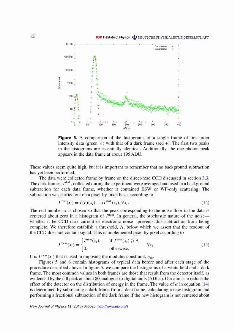
Figure 5. A comparison of the histograms of a single frame of first-orderintensity data (green ×) with that of a dark frame (red +). The first two peaksin the histograms are essentially identical. Additionally, the one-photon peakappears in the data frame at about 195 ADU.

These values seem quite high, but it is important to remember that no background subtractionhas yet been performed.

The data were collected frame by frame on the direct-read CCD discussed in section 3.3.The dark frames, I dark

i , collected during the experiment were averaged and used in a backgroundsubtraction for each data frame, whether it contained ESW or WF-only scattering. Thesubtraction was carried out on a pixel-by-pixel basis according to

I treat(xi)= I (r)(xi)−α I dark(xi),∀xi . (14)

The real number α is chosen so that the peak corresponding to the noise floor in the data iscentered about zero in a histogram of I treat. In general, the stochastic nature of the noise—whether it be CCD dark current or electronic noise—prevents this subtraction from beingcomplete. We therefore establish a threshold, 3, below which we assert that the readout ofthe CCD does not contain signal. This is implemented pixel by pixel according to

I meas(xi)=

{I treat(xi), if I treat(xi)>3

0, otherwise.∀xi , (15)

It is I meas(xi) that is used in imposing the modulus constraint, πm.Figures 5 and 6 contain histograms of typical data before and after each stage of the

procedure described above. In figure 5, we compare the histograms of a white field and a darkframe. The most common values in both frames are those that result from the detector itself, asevidenced by the tall peak at about 80 analogue-to-digital units (ADUs). Our aim is to reduce theeffect of the detector on the distribution of energy in the frame. The value of α in equation (14)is determined by subtracting a dark frame from a data frame, calculating a new histogram andperforming a fractional subtraction of the dark frame if the new histogram is not centered about

New Journal of Physics 12 (2010) 035020 (http://www.njp.org/)

13

1

01

001

0001

00001

000001

60+e1

05- 0 05 001 051 002 052

Occ

uran

ce

ADUs

noitcartbus cisaBnoitcartbus evitagen-noNnoitcartbus dedlohserhT

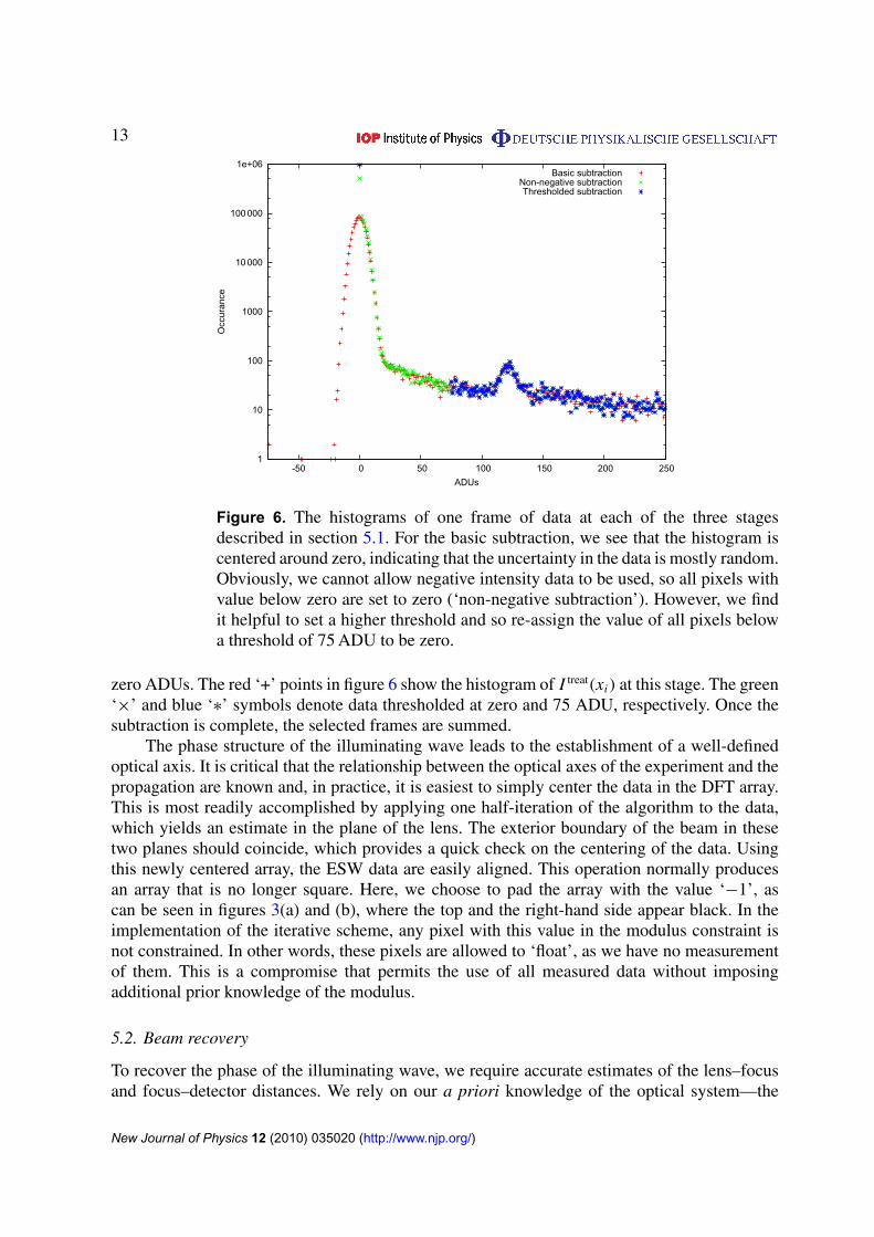
Figure 6. The histograms of one frame of data at each of the three stagesdescribed in section 5.1. For the basic subtraction, we see that the histogram iscentered around zero, indicating that the uncertainty in the data is mostly random.Obviously, we cannot allow negative intensity data to be used, so all pixels withvalue below zero are set to zero (‘non-negative subtraction’). However, we findit helpful to set a higher threshold and so re-assign the value of all pixels belowa threshold of 75 ADU to be zero.

zero ADUs. The red ‘+’ points in figure 6 show the histogram of I treat(xi) at this stage. The green‘×’ and blue ‘∗’ symbols denote data thresholded at zero and 75 ADU, respectively. Once thesubtraction is complete, the selected frames are summed.

The phase structure of the illuminating wave leads to the establishment of a well-definedoptical axis. It is critical that the relationship between the optical axes of the experiment and thepropagation are known and, in practice, it is easiest to simply center the data in the DFT array.This is most readily accomplished by applying one half-iteration of the algorithm to the data,which yields an estimate in the plane of the lens. The exterior boundary of the beam in thesetwo planes should coincide, which provides a quick check on the centering of the data. Usingthis newly centered array, the ESW data are easily aligned. This operation normally producesan array that is no longer square. Here, we choose to pad the array with the value ‘−1’, ascan be seen in figures 3(a) and (b), where the top and the right-hand side appear black. In theimplementation of the iterative scheme, any pixel with this value in the modulus constraint isnot constrained. In other words, these pixels are allowed to ‘float’, as we have no measurementof them. This is a compromise that permits the use of all measured data without imposingadditional prior knowledge of the modulus.

5.2. Beam recovery

To recover the phase of the illuminating wave, we require accurate estimates of the lens–focusand focus–detector distances. We rely on our a priori knowledge of the optical system—the

New Journal of Physics 12 (2010) 035020 (http://www.njp.org/)

14

zone plate diameter and outermost zone width, as well as the photon energy are known—andthe magnification argument presented in section 4.2. We strictly enforce the known size of thezone plate through the application of the support constraint in the lens plane in the algorithmdescribed in section 2.2.1.

The experimental parameters corresponding to the data here were

• wavelength: λ= 6.78 Å

• zone plate diameter: D = 160µm

• outermost zone width: 1r = 50 nm

• focal length: f =D1rλ

= 11.8 mm

• detector distance: L = 0.509 m.

In figure 2(b), we display the magnitude of the reconstructed, illuminating wave in the plane ofthe sample. This is the result of propagating the estimate that resulted from 300 iterations of thealgorithm. It is immediately obvious that the wave overfills the DFT unit cell and, due to theperiodic boundary conditions, ‘folds over’ on the edges of the discrete array. This is one ofthe problems that can be avoided by performing the subtraction of the complex illuminatingwave as described in section 2.2.2.

5.3. ESW recovery

In addition to a knowledge of the geometry discussed above, we now require the result ofthe previous section to proceed with the reconstruction of the ESW. The phased far-fieldillumination is multiplied by an additional spherical phase factor so that propagation betweenthe detector and sample planes may be accomplished by means of the FFT. The sample–focusdistance is estimated, as discussed in section 3.3, to be 1.13 mm. This and other geometricalfactors can be varied to choose the plane in which the sample-plane reconstruction is formedand it is often useful to do so within the experimental error of their measurement. With thisinformation in hand, we apply the algorithm of section 2.2.2.

The estimate of the wave[T(r s)− 1

]ψ(r s, zs) on the kth iteration can then be constrained

by a support. The shadow image of the sample provides an immediate estimate of the fractionof the beam it occupies and its shape. In the current example, we chose to employ a supportthat starts with the size and shape estimated from the shadow image and gradually shrink it bythresholding at 11% of its value and convolving the result with a Gaussian function of variance1 pixel. After 30 iterations, this procedure was halted and the support remained fixed for thenext 270 iterations, although acceptable convergence was probably obtained after 100.

The magnitude of[T(r s)− 1

]ψ(r s, zs) is shown for the two subsets of the data discussed

above in figure 7. By accepting data with R > 0.9959, 89 of 800 frames are summed andreconstructed to yield figure 7(a), the magnitude, and 7(b), the phase. With R = 0.9957, 272frames are summed and the magnitude of the recovered wave is shown in figure 7(c). Use of thelatter data clearly results in an image that is of lower quality than the former. We attribute thedifference between the two results to a change in the experimental geometry. The most likelycause is a slow drift of the sample with respect to the optic, as these are not thermally controlled.It is also possible that some property of the beamline or the source has changed, but these arenot obvious from an examination of white-field data taken before and after the ESW data.

The reconstruction itself is of high quality. Interestingly, in addition to the expected chevronpattern, three other objects have appeared in the reconstructed wave. We believe these to be dust

New Journal of Physics 12 (2010) 035020 (http://www.njp.org/)

15

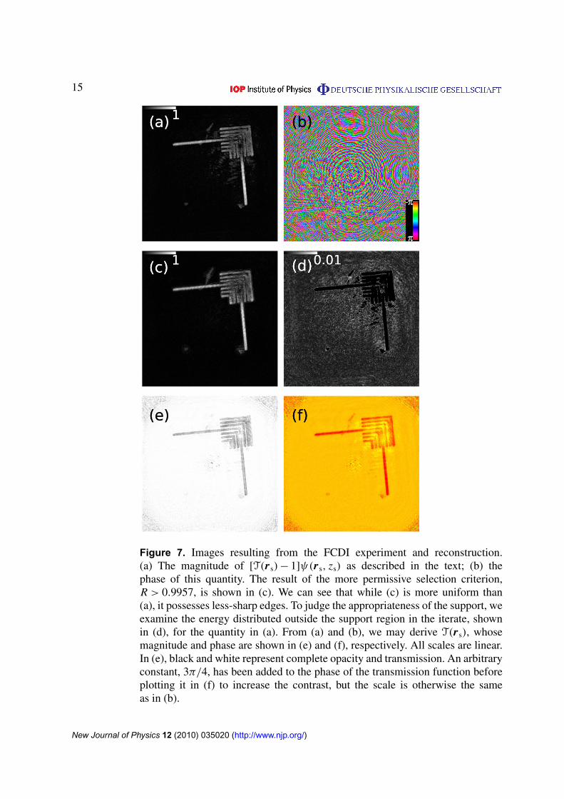
Figure 7. Images resulting from the FCDI experiment and reconstruction.(a) The magnitude of [T(r s)− 1]ψ(r s, zs) as described in the text; (b) thephase of this quantity. The result of the more permissive selection criterion,R > 0.9957, is shown in (c). We can see that while (c) is more uniform than(a), it possesses less-sharp edges. To judge the appropriateness of the support, weexamine the energy distributed outside the support region in the iterate, shownin (d), for the quantity in (a). From (a) and (b), we may derive T(r s), whosemagnitude and phase are shown in (e) and (f), respectively. All scales are linear.In (e), black and white represent complete opacity and transmission. An arbitraryconstant, 3π/4, has been added to the phase of the transmission function beforeplotting it in (f) to increase the contrast, but the scale is otherwise the sameas in (b).

New Journal of Physics 12 (2010) 035020 (http://www.njp.org/)

16

or other, weakly scattering contaminants on the sample. They are dimly visible in a scanning-x-ray micrograph, but not present in a scanning-electron one. We assign a resolution to thisimage of 24nm, which is derived from Abbe theory [18] as described in [12].

It is instructive to ask what features of the estimated ESW are being suppressed by theapplication of the support. For this purpose, we examine that portion of the estimate that fallswithin the complement to the support. Figure 7(d) is the magnitude of this portion of the estimateon the penultimate iteration of the procedure, whose result is shown in figure 7(a). The scale barshows that the largest single pixel in this array is 1% of the greatest value in the estimate. Fromthis we observe that the threshold has been set so high as to forbid the contribution of someweakly scattering areas to the ESW on each iteration. In particular, the fiber along the upperarm of the chevron was rendered discontinuous by the shrinking support, whereas some energyis clearly present in the unconstrained estimate. This is consistent with figure 7(c), where theseobjects have not been cut into by the thresholding, probably because the energy of the estimateis more evenly distributed in this blurry image.

In order to make a connection between the object reconstructed using this approach and itsphysical properties via the index of refraction, it is necessary to process the estimate to recoverT(r). The magnitude and phase of this quantity are shown in figures 7(e) and (f). The expectedresult is that all areas outside the object of interest should have unit magnitude and zero phaseshift. In figure 7(e), all pixels of unity or greater are white. All areas outside the region occupiedby the illuminating wave, shown in figure 2(b), have no physical meaning. Similarly, near theoptical axis, which passes through the center of the array, the illumination approaches zeroand oscillates rapidly. In these two regions, the magnitude of the pixel may exceed unity bytwo orders of magnitude; however, within the region well illuminated, the distribution of pixelvalues outside the object narrowly peaks at unity. On this color scale, black would represent notransmission and hence we see that the Au object appears gray and the weakly scattering objectsare difficult to discern. For ease of display in figure 7(f), we have added a phase of 3π/4 becausethe unaltered phase represented on the scale bar in figure 7(b) provides little contrast in print.

6. Conclusion

We have provided a detailed description of the algorithmic and experimental considerationsspecific to FCDI. The technique has algorithmic and experimental advantages over its plane-wave progenitor. The uniqueness relation [13] between the detector-plane wave and itsdiffraction pattern manifests itself in the fast and reliable convergence of the iterative algorithms.The requirement for achieving these benefits is that one must understand the detailed nature ofthe illuminating wave and the experimental geometry.

Because the wave illuminating the sample is diverging, the intensity due to the incidentradiation is spread over a large region of the detector. This has two practical benefits: there is nomissing data as the experiment does not require a beam stop to protect the 2D detector, and theinterference between the in-line holographs can be sampled in the detector. By establishing anoptical axis in the experiment, one destroys the translational invariance enjoyed by plane-waveCDI. We believe that this is a small cost for the benefits provided by the experimental geometry.

The underlying principle of FCDI—that one should exploit explicit knowledge of the waveincident upon the sample and the experimental geometry—is likely to become increasinglyimportant in CDI as new sources, such as x-ray-free-electron lasers [28, 29], becomeavailable.

New Journal of Physics 12 (2010) 035020 (http://www.njp.org/)

17

Acknowledgments

We thank Ian McNulty, Brian Abbey, Mark Pfeifer, David Paterson and Martin DeJongefor useful discussions and assistance with experimental work. All the authors of this workacknowledge the support of the Australian Research Council Centres (ARC) of Excellenceprogram. KAN acknowledges the support of an ARC Federation Fellowship. We acknowledgetravel funding provided by the International Synchrotron Access Program (ISAP) managedby the Australian Synchrotron. The ISAP is funded by a National Collaborative ResearchInfrastructure Strategy grant provided by the Federal Government of Australia Use of theAdvanced Photon Source at Argonne National Laboratory was supported by the US Departmentof Energy, Office of Science, Office of Basic Energy Sciences, under contract no. DE-AC02-06CH11357.

References

[1] Miao J, Charalambous P, Kirz J and Sayre D 1999 Extending the methodology of x-ray crystallography toallow imaging of micrometre-sized non-crystalline specimens Nature 400 342–4

[2] Miao J, Hodgson K O, Ishikawa T, Larabell C A, LeGros M A and Nishino Y 2003 Imaging wholeEscherichia coli bacteria by using single-particle x-ray diffraction Proc. Natl Acad. Sci. USA 100 10–2

[3] Shapiro D et al 2005 Biological imaging by soft x-ray diffraction microscopy Proc. Natl Acad. Sci. USA102 15343–6

[4] Williams G J et al 2008 High-resolution x-ray imaging of plasmodium falciparum-infected red blood cellsCytometry A 73 949–57

[5] Nishino Y, Takahashi Y, Imamoto N, Ishikawa T and Maeshima K 2009 Three-dimensional visualization ofa human chromosome using coherent x-ray diffraction Phys. Rev. Lett. 102 018101

[6] Barty A et al 2008 Three-dimensional coherent x-ray diffraction imaging of a ceramic nanofoam:determination of structural deformation mechanisms Phys. Rev. Lett. 101 055501

[7] Robinson I K, Vartanyants I A, Williams G J, Pfeifer M A and Pitney J A 2001 Reconstruction of the shapesof gold nanocrystals using coherent x-ray diffraction Phys. Rev. Lett. 87 195505

[8] Williams G J, Pfeifer M A, Vartanyants I A and Robinson I K 2003 Three-dimensional imaging ofmicrostructure in Au nanocrystals Phys. Rev. Lett. 90 175501

[9] Pfeifer M A, Williams G J, Vartanyants I A, Harder R and Robinson I K 2006 Three-dimensional mapping ofa deformation field inside a nanocrystal Nature 442 63–6

[10] Thibault P, Dierolf M, Menzel A, Bunk O, David C and Pfeiffer F 2008 High-resolution scanning x-raydiffraction microscopy Science 321 379–82

[11] Whitehead L W, Williams G J, Quiney H M, Vine D J, Dilanian R A, Flewett S, Nugent K A, Peele A G,Balaur E and McNulty I 2009 Diffractive imaging using partially coherent x-rays Phys. Rev. Lett. 103243902

[12] Williams G J, Quiney H M, Dhal B B, Tran C Q, Nugent K A, Peele A G, Paterson D and de Jonge M D 2006Fresnel coherent diffractive imaging Phys. Rev. Lett. 97 025506

[13] Pitts T A and Greenleaf J F 2003 Fresnel transform phase retrieval from magnitude IEEE Trans. Ultrason.Ferroelectr. Freq. Control 8 1035–45

[14] Bates R H T 1982 Fourier phase problems are uniquely solvable in more than one dimension. I: Underlyingtheory Optik 61 247–62

[15] Abbey B, Nugent K A, Williams G J, Clark J N, Peele A G, Pfeifer M A, de Jonge M and McNulty I 2008Keyhole coherent diffractive imaging Nat. Phys. 4 394–8

[16] Abbey B, Williams G J, Pfeifer M A, Clark J N, Putkunz C T, Torrance A, McNulty I, Levin T M, PeeleA G and Nugent K A 2008 Quantitative coherent diffractive imaging of an integrated circuit at a spatialresolution of 20 nm Appl. Phys. Lett. 93 214101

New Journal of Physics 12 (2010) 035020 (http://www.njp.org/)

18

[17] Clark J N, Williams G J, Quiney H M, Whitehead L, de Jonge M D, Hanssen E, Altissimo M, Nugent K A andPeele A G 2008 Quantitative phase measurement in coherent diffraction imaging Opt. Express 16 3342–8

[18] Born M and Wolf E 1999 Principles of Optics: Electromagnetic Theory of Propagation, Interference andDiffraction of Light 7th edn (Cambridge: Cambridge University Press)

[19] Berry M V 1971 Diffraction in crystals at high energies J. Phys. C: Solid State Phys. 4 697–722[20] Gerchberg R W and Saxton W O 1972 A practical algorithm for the determination of phase from image and

diffraction plane pictures Optik 35 237–46[21] Bauschke H H, Combettes P L and Luke D R 2002 On the structure of some phase retrieval algorithms Proc.

IEEE Int. Conf. Image Processing vol 2 pp 841–4[22] Elser V 2003 Phase retrieval by iterated projections J. Opt. Soc. Am. A 20 40–55[23] Fienup J R 1982 Phase retrieval algorithms: a comparison Appl. Opt. 21 2758–69[24] Marchesini S, He H, Chapman H N, Hau-Riege S P, Noy A, Howells M R, Weierstall U and Spence J C H

2003 X-ray image reconstruction from a diffraction pattern alone Phys. Rev. B 68 140101[25] Quiney H M, Peele A G, Cai Z, Paterson D and Nugent K A 2006 Diffractive imaging of highly focused x-ray

fields Nat. Phys. 2 101–6[26] Quiney H M, Nugent K A and Peele A G 2005 Iterative image reconstruction algorithms using wave-front

intensity and phase variation Opt. Lett. 30 1638–40[27] McNulty I, Khounsary A, Feng Y P, Qian Y, Barraza J, Benson C and Shu D 1996 A beamline for 1–4 keV

microscopy and coherence experiments at the advanced photon source Rev. Sci. Instrum. 67 3372–2[28] Feldhaus J, Arthur J and Hastings J B 2005 X-ray free-electron lasers J. Phys. B: At. Mol. Opt. Phys.

38 S799–819[29] Chapman H N et al 2006 Femtosecond diffractive imaging with a soft-x-ray free-electron laser Nat. Phys.

2 839–43

New Journal of Physics 12 (2010) 035020 (http://www.njp.org/)