Embed Size (px)
Citation preview
FRIEZES SATISFYING HIGHER SLk-DETERMINANTS
KARIN BAUR, ELEONORE FABER, SIRA GRATZ, KHRYSTYNA SERHIYENKO, GORDANATODOROV
Abstract. In this article, we construct SLk-friezes using Plucker coordinates, makinguse of the cluster structure on the homogeneous coordinate ring of the Grassmannianof k-spaces in n-space via the Plucker embedding. When this cluster algebra is of finitetype, the SLk-friezes are in bijection with the so-called mesh friezes of the correspondingGrassmannian cluster category. These are collections of positive integers on the AR-quiver of the category with relations inherited from the mesh relations on the category.In these finite type cases, many of the SLk-friezes arise from specialising a cluster to 1.These are called unitary. We use Iyama-Yoshino reduction to analyse the non-unitaryfriezes. With this, we provide an explanation for all known friezes of this kind. Anappendix by Cuntz and Plamondon proves that there are 868 friezes of type E6.
Contents
1. Introduction 2
2. Background and notation 3
3. Integral tame SLk-friezes from Plucker friezes 10
4. Connection between the categories C(k, n) and SLk-friezes 15
5. Mesh friezes via IY-reduction 29
Appendix A. Proof of Proposition 3.5 37
Appendix B. Counting friezes in type E6 42
Date: April 24, 2020.2010 Mathematics Subject Classification. 05E10, 13F60, 16G20, 18D99, 14M15 .Key words and phrases. frieze pattern, mesh frieze, unitary frieze, cluster category, Grassmannian,
Iyama–Yoshino reduction.K.B. was supported by FWF grants P 30549-N26 and W1230. She is supported by a Royal Society
Wolfson Research Merit Award. E.F. is a Marie Sk lodowska-Curie fellow at the University of Leeds (fundedby the European Union’s Horizon 2020 research and innovation programme under the Marie Sk lodowska-Curie grant agreement No 789580). K.S. was supported by NSF Postdoctoral Fellowship MSPRF - 1502881.
1
arX
iv:1
810.
1056
2v2
[m
ath.
RA
] 2
2 A
pr 2
020
2 K. BAUR, E. FABER, S. GRATZ, K. SERHIYENKO, G. TODOROV
1. Introduction
In this paper, we establish an explicit connection between SLk-friezes and Grassmannian
cluster categories and algebras.
Integral SLk-friezes are certain arrays of integers consisting of finitely many rows of infinite
length, see Example 2.4. Moreover, entries in an SLk frieze satisfy the so-called diamond
rule, where for every k×k diamond formed by the neighboring entries, the determinant of
the corresponding matrix equals 1. For example, when k = 2 each diamonda
b cd
satisfies
the relation∣∣ b ad c
∣∣ = 1. Moreover, we consider tame SLk frieze, that is friezes where the
determinant of every (k + 1) × (k + 1) diamond is 0. Such friezes have horizontal period
n, where n is determined by k and the number of rows.
SLk-friezes were introduced in the seventies by Coxeter [Cox71] in the case k = 2, while
higher SLk-frieze patterns first appeared in work of Cordes-Roselle [CR72]. Conway and
Coxeter further studied SL2-friezes in [CC73a, CC73b], where they showed that there
exists a bijection between SL2 friezes and triangulations of polygons. Interest in friezes
and their various generalizations renewed after the introduction of cluster algebras in 2001,
as cluster algebras coming from the Grassmannian of 2 planes in an n-dimensional space
are also in bijection with triangulations of polygons. Moreover, it was shown later that
SL2 friezes can be obtained by specializing all cluster variables in a given cluster to one
[CC06].
In this way, SL2 friezes are well-understood and they are closely related to the combi-
natorics of cluster algebras. On the other hand, the classification of integral SLk-friezes
remains elusive. Our paper makes a step in the direction of a complete classification. We
show that in the finite type cases, all integral SLk-friezes can be obtained from the combi-
natorics of the cluster algebras on coordinate rings of Grassmannians, and Grassmannian
cluster categories. We make use of the combinatorial tools that we call Plucker friezes,
which arise from the cluster algebras, and mesh friezes, which arise from Grassmannian
cluster categories.
Plucker friezes play a crucial role in our construction of SLk-friezes. Their entries are given
by a constellation of Plucker coordinates in the homogeneous coordinate ring A(k, n) of
the Grassmannian Gr(k, n) via the Plucker embedding. We show that the (specialized)
Plucker frieze of type (k, n) deserves its name: it is indeed an SLk-frieze – all its k × kdiamonds have determinant 1 (cf. Theorem 3.1). In particular, each map from A(k, n)
to Z, given by a specialization of a cluster to one, yields a tame integral SLk-frieze (cf.

FRIEZES SATISFYING HIGHER SLk-DETERMINANTS 3
Corollary 3.12). We call friezes obtained in this way unitary. This generalizes the results
about friezes from the case k = 2, which have been well-known and studied for some time:
Indeed, all SL2-friezes arise from the (specialized) Plucker frieze of type (2, n) in this way.
However, for k > 2 not all friezes are unitary.
Next, we use categorification of cluster algebras to obtain all SLk friezes whenever A(k, n)
is of finite type. A mesh frieze is an integral frieze on the Auslander-Reiten quiver of
a Grassmannian cluster category such that entries coming from a mesh satisfy a certain
frieze-like relation. In the case k = 2, a mesh frieze of the cluster category exactly
agrees with the SL2-frieze. Thus, in light of the connection that we found, it makes sense
to consider relationship between SLk-friezes and mesh friezes of Grassmannian cluster
categories for k > 2. In finite type we show that there exists a bijection between the two.
In particular, this implies that in finite type every SLk frieze is obtained by specializing
the collection of cluster variables in a given cluster to some set of positive integers.
This also allows us to use tools from representation theory, such as Iyama-Yoshino reduc-
tion, to study SLk-friezes. It enables us to pass from a mesh frieze of a given “rank” (that
is, a mesh frieze for a cluster category whose rank is given by the number of indecompos-
ables in a cluster tilting object), to one of lower rank. Making use of known restrictions
for smaller rank cases (in particular, of type A cases) we can then draw conclusions about
the nature of our original mesh frieze. The natural bijection, in finite type cases, between
mesh friezes and SLk-friezes means that Iyama-Yoshino reduction helps us better our un-
derstanding of integral SLk-friezes. In particular, we obtain new results on the number of
such friezes and their possible entries.
An appendix by Cuntz and Plamondon determines the number of friezes in type (3, 7).
Acknowledgements. We want to thank Hugh Thomas for comments on an earlier ver-
sion of the paper. We also want to thank the two anonymous referees for their helpful
comments and suggestions.
2. Background and notation
2.1. SLk-friezes.

4 K. BAUR, E. FABER, S. GRATZ, K. SERHIYENKO, G. TODOROV
Definition 2.1. Let R be an integral domain.
An SLk-frieze (over R) is a grid in the plane, consisting of a finite number of rows:
0 0 0 0 0 0 0
. . . . ..
. ..
. ..
. ..
. ..
. ..
. . .
0 0 0 0 0 0 0
. . . 1 1 1 1 1 1 . . .
∗ ∗ ∗ m0,w−1 m1,w m2,w+1 ∗. ..
. . . . . . m01 m12 m23 m34 . . .. . . m00 m11 m22 m33 . . . . . .
1 1 1 1 1 1 1
. . . 0 0 0 0 0 0 . . .
. ..
. ..
. ..
. ..
. ..
. . . 0 0 0 0 0 0
The frieze is formed by k − 1 rows of zeroes followed by a row of 1s from top and from
bottom respectively and by w ≥ 1 rows of elements mij ∈ R in between, such that every
k × k-diamond of entries of the frieze has determinant 1, i.e. , whenever we consider a
matrix having k successive entries of a row of an SLk-frieze on its diagonals and all other
entries above and below the diagonal accordingly, the determinant of this matrix is 1. The
integer w is called the width of the frieze.
Definition 2.2. Let F be an SLk-frieze over R.
(1) F is tame if all (k + 1) × (k + 1)-diamonds in F have determinant 0. In general,
we define an s × s-diamond of the frieze, where 1 ≤ s ≤ k + 1, as the matrix having s
successive entries of the frieze on its diagonals and all other entries above and below the
diagonal accordingly.
(2) If all non-trivial entries mij with 0 ≤ i, j ≤ w of F are positive integers, we call F an
integral SLk-frieze.
Remark 2.3. One can prove that every tame SLk-frieze of width w over a field K has
horizontal period n = w + k + 1, which was first proven for certain SLk-friezes in [CR72]
and in general in [MGOST14, Cor. 7.1.1].
SL2-friezes were first studied by Coxeter and Conway–Coxeter in the early 1970s, see
Example 2.4 below. Higher SLk-frieze patterns made their first appearance 1972 in work
of Cordes–Roselle [CR72] (with extra conditions on the minors of the first k×k-diamonds)
FRIEZES SATISFYING HIGHER SLk-DETERMINANTS 5
and seem only to have re-emerged with the introduction of cluster algebras: as 2-friezes
[Pro05], SLk-tilings in [BR10] and more systematically in [MGOT12, MGOST14, MG12,
Cun17]. See also [MG15] for a survey on different types of frieze patterns.
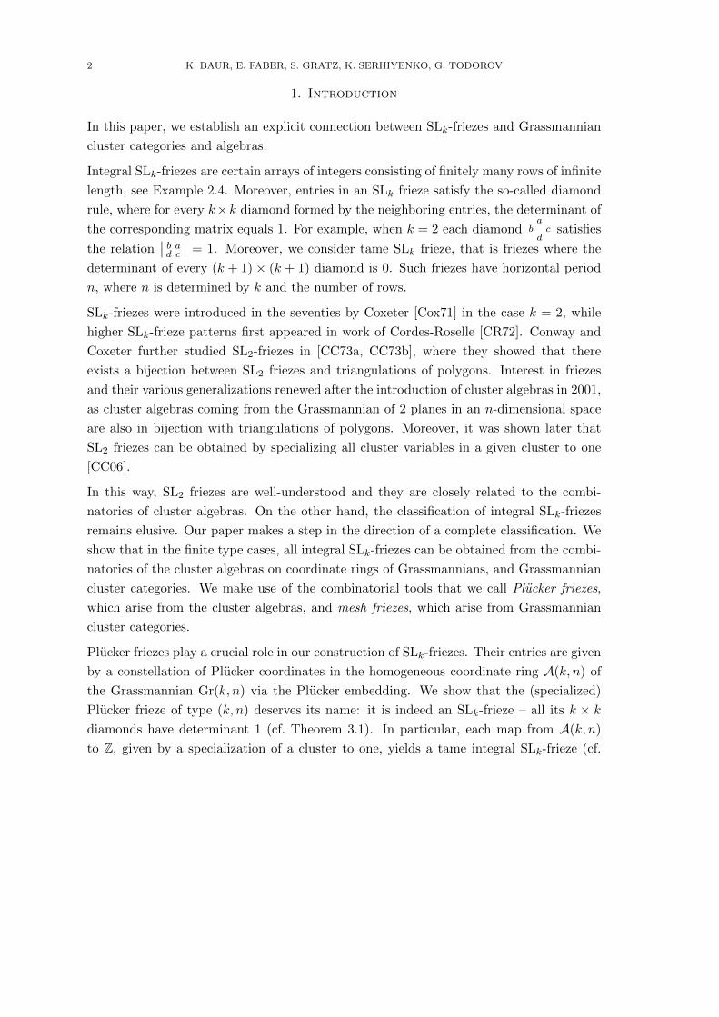
Example 2.4. An SL2-frieze is simply called a frieze pattern. Frieze patterns have first
been studied by Coxeter, [Cox71] and by Conway and Coxeter in [CC73a, CC73b]. They
showed that integral frieze patterns of width w are in bijection with triangulations of
w+ 3-gons. Their horizontal period is w+ 3 or a divisor of w+ 3. The following example
4
1
22
2
1
0 0 0 0 0 0 0
1 1 1 1 1 1 11
1
3
1 1 1 1 1 1 11
0 0 0 0 0 0 0
4 11222
2 1 2 224
3 3
1
1 3 1 3 1
: : :
: : :
: : :
: : :
arises from a fan triangulation of a hexagon: The first non-trivial row of the frieze pattern
(in bold face) is given by the number of triangles of the triangulation meeting at the
vertices of the hexagon (counting these while going around the hexagon).
2.2. Plucker relations.
Throughout, we fix k, n ∈ Z>0 with 2 ≤ k ≤ n2 and consider the Grassmannian Gr(k, n)
as a projective variety via the Plucker embedding, with homogeneous coordinate ring
A(k, n) = C[Gr(k, n)].
This coordinate ring can be equipped with the structure of a cluster algebra as we briefly
recall here. For details, we refer to [Sco06].
We write [1, n] = {1, 2, . . . , n} for the closed interval of integers between 1 and n. A
k-subset of [1, n] is a k-element subset of [1, n]. Every k-subset I = {i1, . . . , ik} with
i1 < · · · < ik of [1, n] gives rise to a Plucker coordinate pi1,i2,...,ik . We extend this definition
to allow different ordering on the indices and repetition of indices: for an arbitrary k-
tuple I = (i1, . . . , ik) we set pi1,...,ik = 0 if there exists ` 6= m such that i` = im and
pi1,...,ik = sgn(π)pj1,...,jk if (i1, . . . , ik) = (j1, . . . , jk), with j1 < j2 < · · · < jk and π is
the permutation sending jm to im for 1 ≤ m ≤ k. Sometimes, by abuse of notation, we
will also call any tuple (i1, . . . , ik) a k-subset. Scott proved in [Sco06] that A(k, n) is a
cluster algebra, where all the Plucker coordinates are cluster variables. For each (k, n),
6 K. BAUR, E. FABER, S. GRATZ, K. SERHIYENKO, G. TODOROV
there exists a cluster consisting of Plucker coordinates and the exchange relations arise
from the Plucker relations (see below).
Note that throughout the article we will consider sets I up to reduction modulo n, where
we choose the representatives 1, . . . , n for the equivalence classes modulo n. If I consists
of k consecutive elements, up to reducing modulo n, we call I a consecutive k-subset and
pI a consecutive Plucker coordinate. These are frozen cluster variables or coefficients, and
we will later set all of them equal to 1. Of importance for our purposes are the Plucker
coordinates which arise from k-subsets of the form I = I0 ∪{m} where I0 is a consecutive
(k − 1)-subset of [1, n] and m is any entry of [1, n] \ I0. We call such k-subsets almost
consecutive. Note that each consecutive k-subset is almost consecutive. In particular the
frozen cluster variables are consecutive and thus almost consecutive.
We follow the exposition of [Mar13, Section 9.2] for the presentation of the Plucker rela-
tions. In the cluster algebra A(k, n), the relations
k∑`=0
(−1)lpi1,...,ik−1,j`pj0,...,j`,...,jk = 0(1)
hold for arbitrary 1 ≤ i1 < i2 < · · · < ik−1 ≤ n and 1 ≤ j0 < j1 < · · · < jk ≤ n,
where · signifies omission. These relations are called the Plucker relations. For k = 2, the
non-trivial Plucker relations are of the form
pa,cpb,d = pa,bpc,d + pa,dpb,c(2)
for arbitrary 1 ≤ a < b < c < d ≤ n. They are often called the three-term Plucker
relations.
Obviously, the order of the elements in a tuple plays a significant role. We will often need
to use ordered tuples, or partially ordered tuples. For this, we introduce the following
notation. For a tuple J = {i1, . . . , i`} of [1, n] and {a1, . . . , a`} = {i1, . . . , i`} with 1 ≤a1 ≤ · · · ≤ a` ≤ n we set
o(J) = o(i1, . . . , i`) = (a1, . . . , a`).
With this notation, if 0 ≤ s, ` ≤ k, we will write pb1,...,bs,o(i1,...,i`),c1,...,ck−`+afor
pb1,...,bs,a1,...,a`,c1,...,ck−`+a. For arbitrary I = {i1, . . . , ik−1} and J = {j0, . . . , jk}, the Plucker
relations (1) then take the form
k∑l=0
(−1)`po(I)j` · po(J\j`) = 0.
FRIEZES SATISFYING HIGHER SLk-DETERMINANTS 7
2.3. Plucker friezes, and special Plucker friezes.
To the homogeneous coordinate ring A(k, n) we now associate a certain frieze pattern
which we will use later to obtain SLk-friezes. It uses the almost consecutive Plucker
coordinates. For brevity, it is convenient to write [r]` for the set {r, r + 1, . . . , r + `− 1}.For example, if k = 4 and n = 9, p[1]3,6 is the short notation for p1236 and po([8]3,4) is short
for p1489.
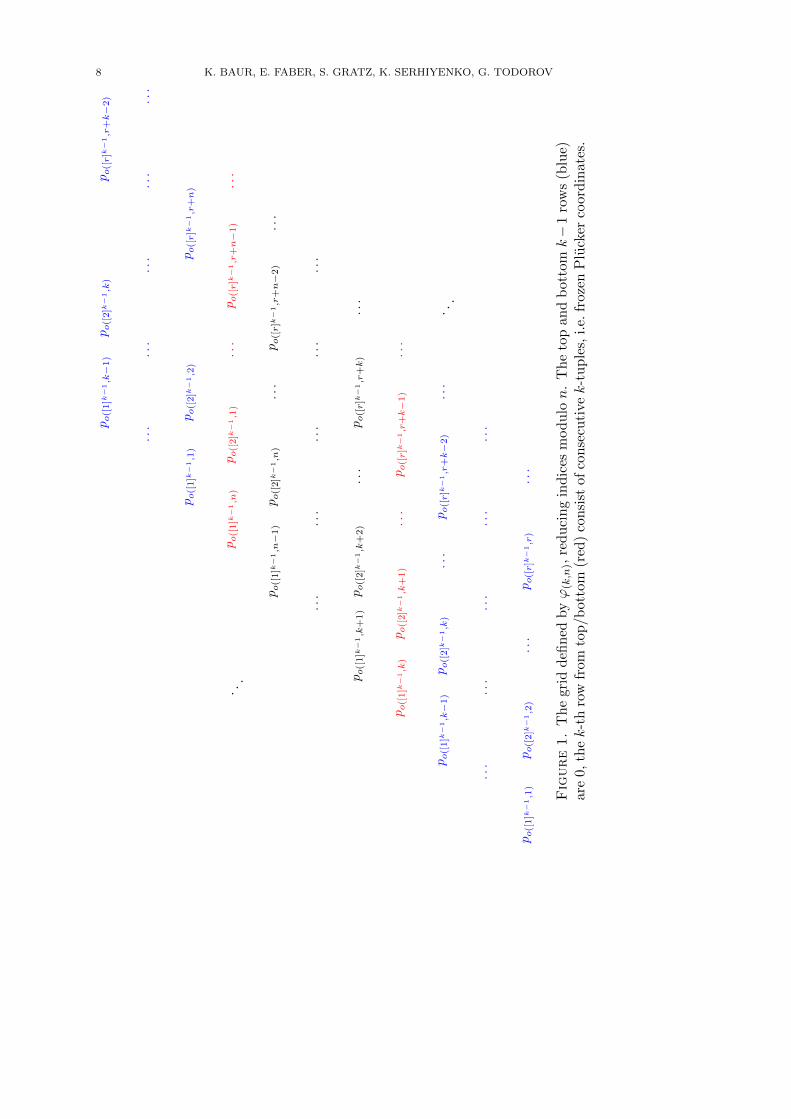
Definition 2.5. The Plucker frieze of type (k, n) is a Z × {1, 2, . . . , n + k − 1}-grid with
entries given by the map
ϕ(k,n) : Z× {1, 2, . . . , n+ k − 1} → A(k, n)
(r,m) 7→ po([r′]k−1,m′),
where r′ ∈ [1, n] is the reduction of r modulo n and m′ ∈ [1, n] is the reduction of m+r′−1
modulo n. We denote the Plucker frieze by P(k,n).
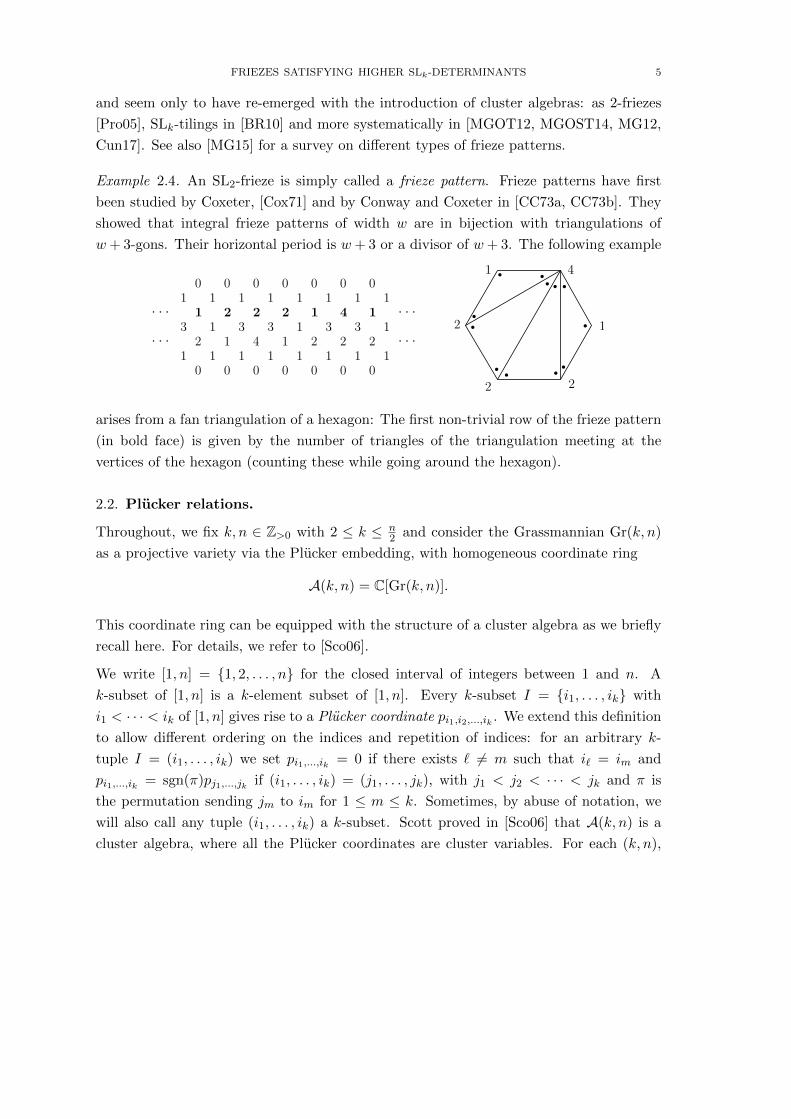
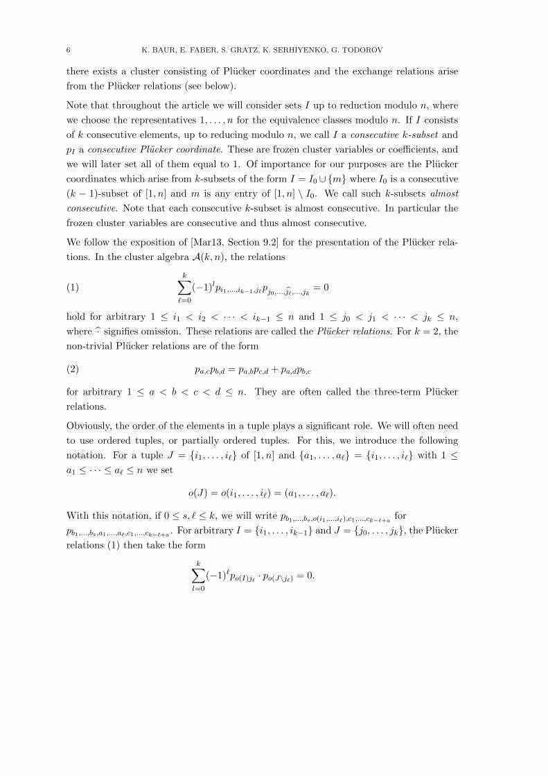
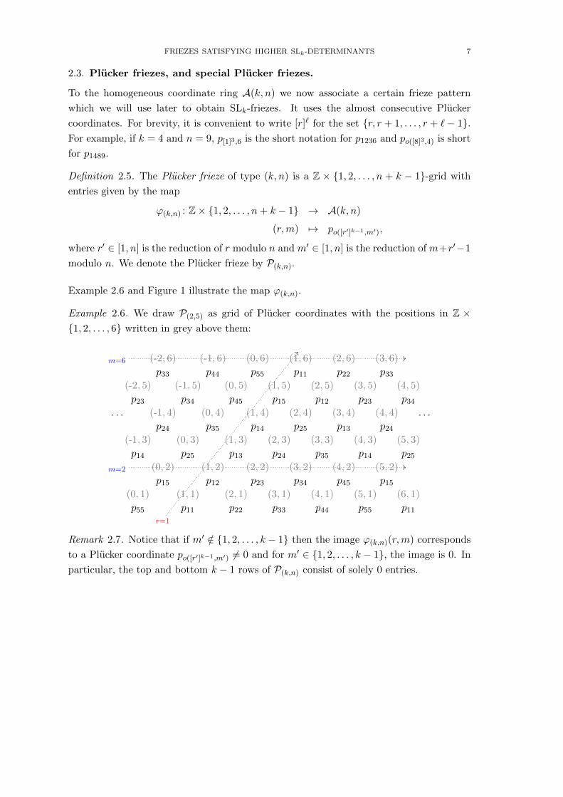
Example 2.6 and Figure 1 illustrate the map ϕ(k,n).
Example 2.6. We draw P(2,5) as grid of Plucker coordinates with the positions in Z ×{1, 2, . . . , 6} written in grey above them:
m=6//(-2, 6) (-1, 6) (0, 6) (1, 6) (2, 6) (3, 6)
p33 p44 p55 p11 p22 p33(-2, 5) (-1, 5) (0, 5) (1, 5) (2, 5) (3, 5) (4, 5)
p23 p34 p45 p15 p12 p23 p34. . . (-1, 4) (0, 4) (1, 4) (2, 4) (3, 4) (4, 4) . . .
p24 p35 p14 p25 p13 p24(-1, 3) (0, 3) (1, 3) (2, 3) (3, 3) (4, 3) (5, 3)
p14 p25 p13 p24 p35 p14 p25
m=2//(0, 2) (1, 2) (2, 2) (3, 2) (4, 2) (5, 2)
p15 p12 p23 p34 p45 p15(0, 1) (1, 1) (2, 1) (3, 1) (4, 1) (5, 1) (6, 1)
p55 p11 p22 p33 p44 p55 p11r=1
BB
Remark 2.7. Notice that if m′ /∈ {1, 2, . . . , k − 1} then the image ϕ(k,n)(r,m) corresponds
to a Plucker coordinate po([r′]k−1,m′) 6= 0 and for m′ ∈ {1, 2, . . . , k − 1}, the image is 0. In
particular, the top and bottom k − 1 rows of P(k,n) consist of solely 0 entries.
8 K. BAUR, E. FABER, S. GRATZ, K. SERHIYENKO, G. TODOROV
po([1]k
−1,1)
po([2]k
−1,2)
po([1]k
−1,k−1)
po([2]k
−1,k)
po([1]k
−1,k)
po([2]k
−1,k+1)
po([1]k
−1,k+1)po([2]k
−1,k+2)
po([1]k
−1,n
−1)
po([2]k
−1,n
)
po([1]k
−1,n
)po([2]k
−1,1)
po([1]k
−1,1)
po([2]k
−1,2)
po([1]k
−1,k−1)
po([2]k
−1,k)
...
...
...
...
...
...
...
...
...
...
...
...
...
...
...
...
...
...
...
...
...
...
...
...
...
...
...
po([r]k
−1,r)
po([r]k
−1,r+k−2)
po([r]k
−1,r+k−1)
po([r]k
−1,r+k)
po([r]k
−1,r+n−2)
po([r]k
−1,r+n−1)
po([r]k
−1,r+n)
po([r]k
−1,r+k−2)
. ..
. ..
Fig
ure
1.
Th
egr
idd
efin
edbyϕ(k,n),
red
uci
ng
ind
ices
modu
lon
.T
he
top
and
bot
tomk−
1ro
ws
(blu
e)ar
e0,
thek-t
hro
wfr
omto
p/b
otto
m(r
ed)
consi
stof
con
secu
tivek-t
up
les,
i.e.
froz
enP
luck
erco
ord
inat
es.
FRIEZES SATISFYING HIGHER SLk-DETERMINANTS 9
Remark 2.8 (Specializing coefficients). In what follows, we will replace all the frozen vari-
ables by 1. For that, let J be the ideal of A(k, n) generated by
{x− 1 | x is a consecutive Plucker coordinate}.
The consecutive Plucker coordinates are precisely the frozen variables in the cluster al-
gebra A(k, n). The quotient A(k, n)/J is a coefficient-free cluster algebra, and there-
fore – as a subring of a field of rational functions over C – an integral domain. Let
s : A(k, n)→ A(k, n)/J be the map induced from the identity on non-consecutive Plucker
coordinates and from replacing the consecutive Plucker coordinates by 1. This map is an
algebra homomorphism A(k, n)→ A(k, n)/J . We write sA(k, n) for A(k, n)/J .
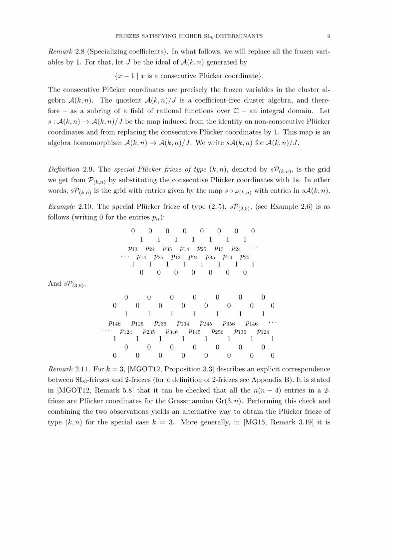
Definition 2.9. The special Plucker frieze of type (k, n), denoted by sP(k,n), is the grid
we get from P(k,n) by substituting the consecutive Plucker coordinates with 1s. In other
words, sP(k,n) is the grid with entries given by the map s ◦ϕ(k,n) with entries in sA(k, n).
Example 2.10. The special Plucker frieze of type (2, 5), sP(2,5), (see Example 2.6) is as
follows (writing 0 for the entries pii):
0 0 0 0 0 0 0 01 1 1 1 1 1 1
p13 p24 p35 p14 p25 p13 p24 · · ·· · · p14 p25 p13 p24 p35 p14 p25
1 1 1 1 1 1 1 10 0 0 0 0 0 0
And sP(3,6):
0 0 0 0 0 0 00 0 0 0 0 0 0 0
1 1 1 1 1 1 1p146 p125 p236 p134 p245 p356 p146 · · ·
· · · p124 p235 p346 p145 p256 p136 p1241 1 1 1 1 1 1 1
0 0 0 0 0 0 00 0 0 0 0 0 0 0
Remark 2.11. For k = 3, [MGOT12, Proposition 3.3] describes an explicit correspondence
between SL3-friezes and 2-friezes (for a definition of 2-friezes see Appendix B). It is stated
in [MGOT12, Remark 5.8] that it can be checked that all the n(n − 4) entries in a 2-
frieze are Plucker coordinates for the Grassmannian Gr(3, n). Performing this check and
combining the two observations yields an alternative way to obtain the Plucker frieze of
type (k, n) for the special case k = 3. More generally, in [MG15, Remark 3.19] it is

10 K. BAUR, E. FABER, S. GRATZ, K. SERHIYENKO, G. TODOROV
observed that, for k ≥ 3, cluster variables for A(k, n) appear as entries in the derived
arrays of an SLk-frieze.
3. Integral tame SLk-friezes from Plucker friezes
3.1. The special Plucker frieze sP(k,n) is a tame SLk-frieze.
In this section, we prove the following result.
Theorem 3.1. The frieze sP(k,n) is a tame SLk-frieze over sA(k, n).
Before we provide a proof for Theorem 3.1, we make some observations on notation and
set-up.
Notation 3.2. Throughout we calculate modulo n. More precisely, we will always reduce
integers modulo n, and identify integers with their representatives in [1, n]. In addition,
the following notation will be useful: For any a, b ∈ [1, n] we denote by [a, b] the closed
interval between a and b modulo n, defined as
[a, b] =
{{p ∈ [1, n] | a ≤ p ≤ b} if a ≤ b{p ∈ [1, n] | a ≤ p ≤ n or 1 ≤ p ≤ b} if b < a,
and by (a, b) the open interval between a and b modulo n, defined as
(a, b) =
{{p ∈ [1, n] | a < p < b} if a ≤ b{p ∈ [1, n] | a < p ≤ n or 1 ≤ p < b} if b < a.
Analogously, we define the half-open intervals [a, b) and (a, b].
Recall that we obtain the frieze sP(k,n) from the frieze P(k,n) by specialising the consecutive
Plucker coordinates to 1. We will compute the determinants of a diamond in the frieze
sP(k,n) via the corresponding diamond in P(k,n). The k×k diamonds in the Plucker frieze
P(k,n) are matrices of the form
A[m]k;r := (po([r+i−1]k−1,m+j−1))1≤i,j≤k,
with
r ∈ [1, n] and m ∈ [r + k − 1, r + n− 1] = [r + k − 1, r − 1],
where as before we calculate modulo n, with representatives 1, . . . , n.
To inductively compute the determinants of the matrices A[m]k;r, we need to consider
other matrices of the following form: For r ∈ [1, n], 1 ≤ s ≤ n and m = (m1, . . . ,ms) with
mi ∈ [1, n] we define
Am;r = (aij)1≤i,j≤s
FRIEZES SATISFYING HIGHER SLk-DETERMINANTS 11
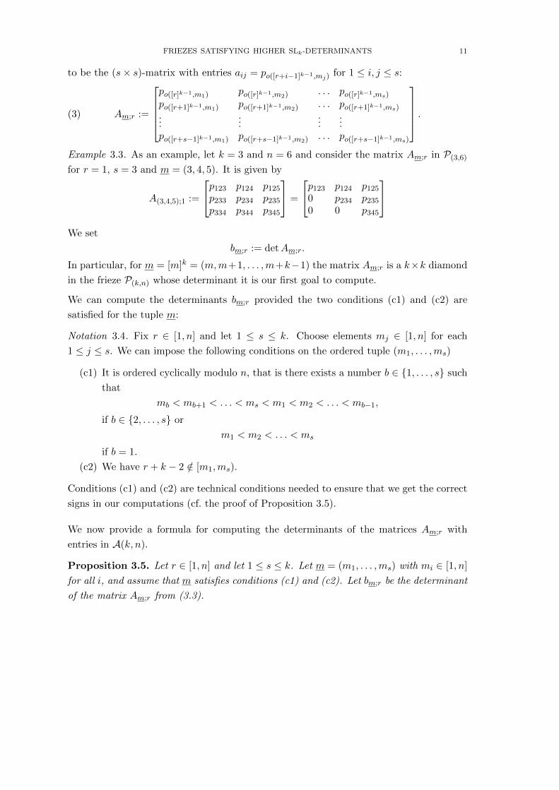
to be the (s× s)-matrix with entries aij = po([r+i−1]k−1,mj) for 1 ≤ i, j ≤ s:
(3) Am;r :=
po([r]k−1,m1) po([r]k−1,m2) . . . po([r]k−1,ms)
po([r+1]k−1,m1) po([r+1]k−1,m2) . . . po([r+1]k−1,ms)...
......
...po([r+s−1]k−1,m1) po([r+s−1]k−1,m2) . . . po([r+s−1]k−1,ms)
.Example 3.3. As an example, let k = 3 and n = 6 and consider the matrix Am;r in P(3,6)for r = 1, s = 3 and m = (3, 4, 5). It is given by
A(3,4,5);1 :=
p123 p124 p125p233 p234 p235p334 p344 p345
=
p123 p124 p1250 p234 p2350 0 p345
We set
bm;r := detAm;r.
In particular, for m = [m]k = (m,m+1, . . . ,m+k−1) the matrix Am;r is a k×k diamond
in the frieze P(k,n) whose determinant it is our first goal to compute.
We can compute the determinants bm;r provided the two conditions (c1) and (c2) are
satisfied for the tuple m:
Notation 3.4. Fix r ∈ [1, n] and let 1 ≤ s ≤ k. Choose elements mj ∈ [1, n] for each
1 ≤ j ≤ s. We can impose the following conditions on the ordered tuple (m1, . . . ,ms)
(c1) It is ordered cyclically modulo n, that is there exists a number b ∈ {1, . . . , s} such
that
mb < mb+1 < . . . < ms < m1 < m2 < . . . < mb−1,
if b ∈ {2, . . . , s} or
m1 < m2 < . . . < ms
if b = 1.
(c2) We have r + k − 2 /∈ [m1,ms).
Conditions (c1) and (c2) are technical conditions needed to ensure that we get the correct
signs in our computations (cf. the proof of Proposition 3.5).
We now provide a formula for computing the determinants of the matrices Am;r with
entries in A(k, n).
Proposition 3.5. Let r ∈ [1, n] and let 1 ≤ s ≤ k. Let m = (m1, . . . ,ms) with mi ∈ [1, n]
for all i, and assume that m satisfies conditions (c1) and (c2). Let bm;r be the determinant
of the matrix Am;r from (3.3).
12 K. BAUR, E. FABER, S. GRATZ, K. SERHIYENKO, G. TODOROV
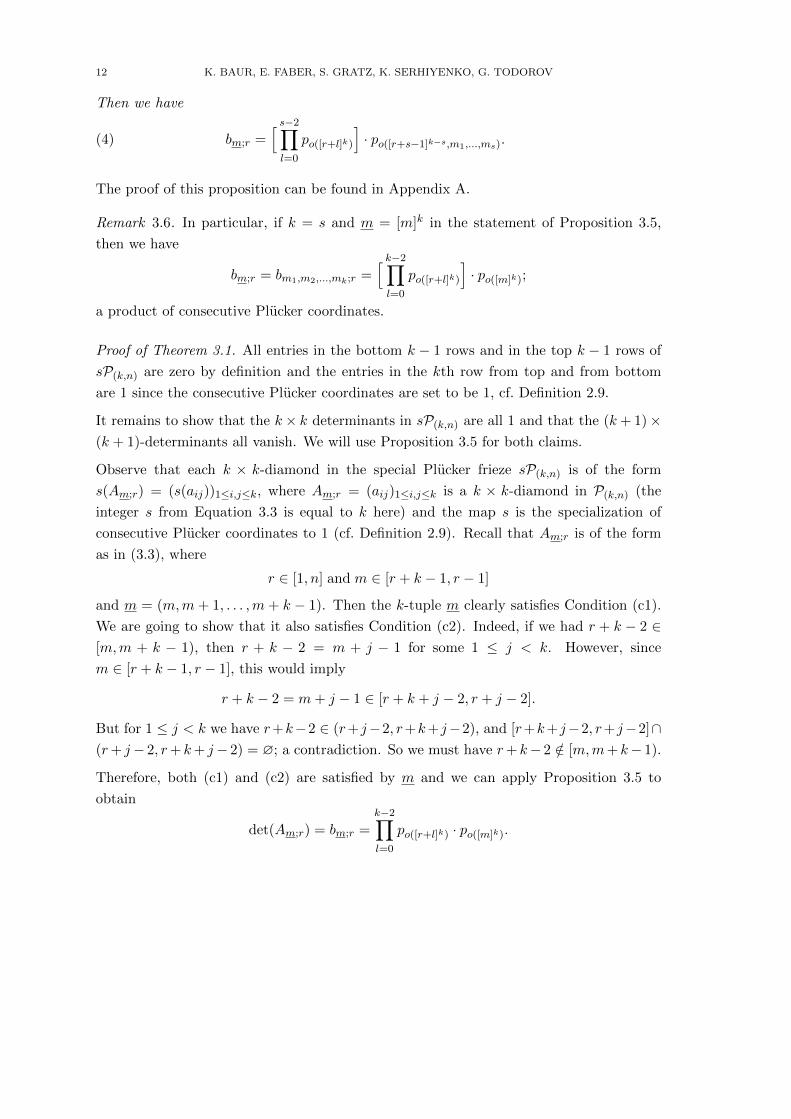
Then we have
bm;r =[ s−2∏l=0
po([r+l]k)
]· po([r+s−1]k−s,m1,...,ms).(4)
The proof of this proposition can be found in Appendix A.
Remark 3.6. In particular, if k = s and m = [m]k in the statement of Proposition 3.5,
then we have
bm;r = bm1,m2,...,mk;r =[ k−2∏l=0
po([r+l]k)
]· po([m]k);
a product of consecutive Plucker coordinates.
Proof of Theorem 3.1. All entries in the bottom k − 1 rows and in the top k − 1 rows of
sP(k,n) are zero by definition and the entries in the kth row from top and from bottom
are 1 since the consecutive Plucker coordinates are set to be 1, cf. Definition 2.9.
It remains to show that the k× k determinants in sP(k,n) are all 1 and that the (k+ 1)×(k + 1)-determinants all vanish. We will use Proposition 3.5 for both claims.
Observe that each k × k-diamond in the special Plucker frieze sP(k,n) is of the form
s(Am;r) = (s(aij))1≤i,j≤k, where Am;r = (aij)1≤i,j≤k is a k × k-diamond in P(k,n) (the
integer s from Equation 3.3 is equal to k here) and the map s is the specialization of
consecutive Plucker coordinates to 1 (cf. Definition 2.9). Recall that Am;r is of the form
as in (3.3), where
r ∈ [1, n] and m ∈ [r + k − 1, r − 1]
and m = (m,m+ 1, . . . ,m+ k − 1). Then the k-tuple m clearly satisfies Condition (c1).
We are going to show that it also satisfies Condition (c2). Indeed, if we had r + k − 2 ∈[m,m + k − 1), then r + k − 2 = m + j − 1 for some 1 ≤ j < k. However, since
m ∈ [r + k − 1, r − 1], this would imply
r + k − 2 = m+ j − 1 ∈ [r + k + j − 2, r + j − 2].
But for 1 ≤ j < k we have r+k−2 ∈ (r+j−2, r+k+j−2), and [r+k+j−2, r+j−2]∩(r+ j− 2, r+ k+ j− 2) = ∅; a contradiction. So we must have r+ k− 2 /∈ [m,m+ k− 1).
Therefore, both (c1) and (c2) are satisfied by m and we can apply Proposition 3.5 to
obtain
det(Am;r) = bm;r =
k−2∏l=0
po([r+l]k) · po([m]k).

FRIEZES SATISFYING HIGHER SLk-DETERMINANTS 13
This yields
det(s(Am;r) = s(bm;r) =
k−2∏l=0
s(po([r+l]k)) · s(po([m]k)) = 1,
for the k × k diamond s(Am;r) of the special Plucker frieze sP(k,n). Since this holds for
every k × k diamond, sP(k,n) is indeed a SLk-frieze.
To show that it is tame, consider an arbitrary (k + 1) × (k + 1) diamond of sP(k,n). It
must be of the form s(A[m]k+1;r) = (s(aij))1≤i,j≤k+1, where A[m]k+1;r is the corresponding
diamond in the Plucker frieze P(k,n) given by (3.3) for [m]k+1 = (m,m+ 1, . . . ,m+k) and
m ∈ [r + k, r − 2]. Similarly to the first part of the proof (for k × k diamonds), one can
show that conditions (c1) and (c2) are satisfied for [m]k+1 and for any order-inheriting
subtuple thereof. So we can apply Proposition 3.5 to compute the determinants bml;r for
ml = (m, . . . , m+ l, . . . ,m+ k), for 0 ≤ l ≤ k, and Laplace expansion for the determinant
of A[m]k+1;r by the last row yields
det(A[m]k+1;r) =k+1∑l=1
(−1)k+1+lpo([r+k]k−1,m+l−1) · bml;r
=k+1∑l=1
(−1)k+1+lpo([r+k]k−1,ml)·k−2∏j=0
po([r+j]k)po(m1,...,ml,...,mk+1)
=k−2∏j=0
po([r+j]k) ·k+1∑l=1
(−1)k+1+lpo([r+k]k−1,ml)po(m1,...,ml,...,mk+1))︸ ︷︷ ︸
(∗)
Now since (*) is precisely the Plucker relation on I = [r + k]k−1 and J = [m1,mk+1], this
term equals zero and so det(A[m]k+1;r) = 0.
It follows that the determinant of the (k + 1)× (k + 1) diamond s(A[m]k+1;r) vanishes,
det(s(A[m]k+1;r)) = s(det(A[m]k+1;r)) = 0,
and thus sP(k,n) is tame. �
Remark 3.7. In [MGOST14, Proposition 3.2.1], it is shown that the variety of SLk-friezes
of width w = n − k − 1, say over C, can be embedded into Gr(k, n) as the subvariety of
points which can be represented by matrices whose consecutive k × k-minors all coincide
(and are non-vanishing). In the strategy from [MGOST14, Proposition 3.2.1], we could
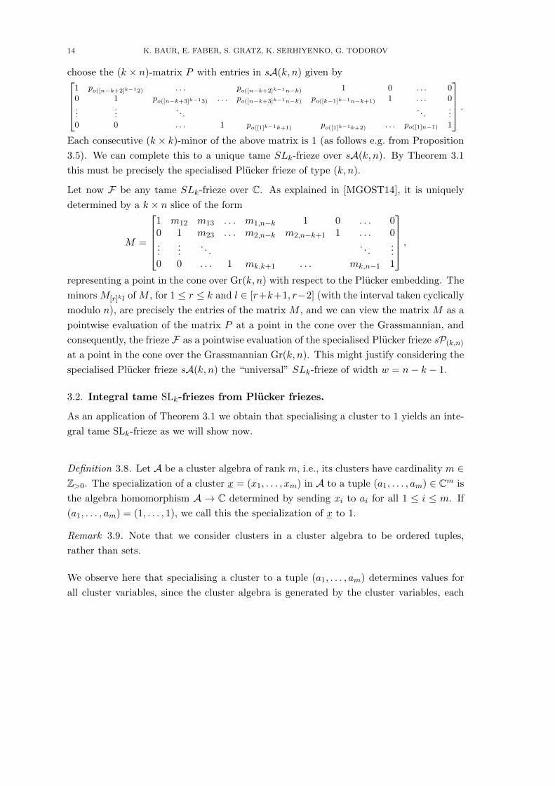
14 K. BAUR, E. FABER, S. GRATZ, K. SERHIYENKO, G. TODOROV
choose the (k × n)-matrix P with entries in sA(k, n) given by1 po([n−k+2]k−12) . . . po([n−k+2]k−1n−k) 1 0 . . . 0
0 1 po([n−k+3]k−13) . . . po([n−k+3]k−1n−k) po([k−1]k−1n−k+1) 1 . . . 0...
.... . .
. . ....
0 0 . . . 1 po([1]k−1k+1) po([1]k−1k+2) . . . po([1]n−1) 1
.Each consecutive (k × k)-minor of the above matrix is 1 (as follows e.g. from Proposition
3.5). We can complete this to a unique tame SLk-frieze over sA(k, n). By Theorem 3.1
this must be precisely the specialised Plucker frieze of type (k, n).
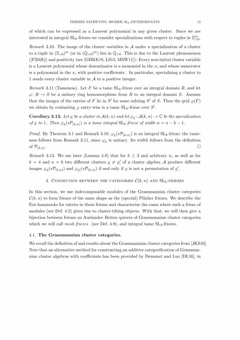
Let now F be any tame SLk-frieze over C. As explained in [MGOST14], it is uniquely
determined by a k × n slice of the form
M =
1 m12 m13 . . . m1,n−k 1 0 . . . 00 1 m23 . . . m2,n−k m2,n−k+1 1 . . . 0...
.... . .
. . ....
0 0 . . . 1 mk,k+1 . . . mk,n−1 1
,representing a point in the cone over Gr(k, n) with respect to the Plucker embedding. The
minors M[r]kl of M , for 1 ≤ r ≤ k and l ∈ [r+k+1, r−2] (with the interval taken cyclically
modulo n), are precisely the entries of the matrix M , and we can view the matrix M as a
pointwise evaluation of the matrix P at a point in the cone over the Grassmannian, and
consequently, the frieze F as a pointwise evaluation of the specialised Plucker frieze sP(k,n)at a point in the cone over the Grassmannian Gr(k, n). This might justify considering the
specialised Plucker frieze sA(k, n) the “universal” SLk-frieze of width w = n− k − 1.
3.2. Integral tame SLk-friezes from Plucker friezes.
As an application of Theorem 3.1 we obtain that specialising a cluster to 1 yields an inte-
gral tame SLk-frieze as we will show now.
Definition 3.8. Let A be a cluster algebra of rank m, i.e., its clusters have cardinality m ∈Z>0. The specialization of a cluster x = (x1, . . . , xm) in A to a tuple (a1, . . . , am) ∈ Cm is
the algebra homomorphism A → C determined by sending xi to ai for all 1 ≤ i ≤ m. If
(a1, . . . , am) = (1, . . . , 1), we call this the specialization of x to 1.
Remark 3.9. Note that we consider clusters in a cluster algebra to be ordered tuples,
rather than sets.
We observe here that specialising a cluster to a tuple (a1, . . . , am) determines values for
all cluster variables, since the cluster algebra is generated by the cluster variables, each
FRIEZES SATISFYING HIGHER SLk-DETERMINANTS 15
of which can be expressed as a Laurent polynomial in any given cluster. Since we are
interested in integral SLk-friezes we consider specializations with respect to tuples in Zm>0.
Remark 3.10. The image of the cluster variables in A under a specialization of a cluster
to a tuple in (Z>0)m (or in (Q>0)
m) lies in Q>0. This is due to the Laurent phenomenon
([FZ02b]) and positivity (see [GHKK18, LS15, MSW11]): Every non-initial cluster variable
is a Laurent polynomial whose denominator is a monomial in the xi and whose numerator
is a polynomial in the xi with positive coefficients . In particular, specialising a cluster to
1 sends every cluster variable in A to a positive integer.
Remark 3.11 (Tameness). Let F be a tame SLk-frieze over an integral domain R, and let
ϕ : R → S be a unitary ring homomorphism from R to an integral domain S. Assume
that the images of the entries of F lie in S′ for some subring S′ of S. Then the grid ϕ(F )
we obtain by evaluating ϕ entry-wise is a tame SLk-frieze over S′.
Corollary 3.12. Let x be a cluster in A(k, n) and let ϕx : A(k, n)→ C be the specialization
of x to 1. Then ϕx(sP(k,n)) is a tame integral SLk-frieze of width w = n− k − 1.
Proof. By Theorem 3.1 and Remark 3.10, ϕx(sP(k,n)) is an integral SLk-frieze; the tame-
ness follows from Remark 3.11, since ϕx is unitary. Its width follows from the definition
of P(k,n). �
Remark 3.13. We see later (Lemma 4.8) that for k ≤ 3 and arbitrary n, as well as for
k = 4 and n = 6 two different clusters x 6= x′ of a cluster algebra A produce different
images ϕx(sP(k,n)) and ϕx′(sP(k,n)) if and only if x is not a permutation of x′.
4. Connection between the categories C(k, n) and SLk-friezes
In this section, we use indecomposable modules of the Grassmannian cluster categories
C(k, n) to form friezes of the same shape as the (special) Plucker friezes. We describe the
Ext-hammocks for entries in these friezes and characterize the cases where such a frieze of
modules (see Def. 4.2) gives rise to cluster-tilting objects. With that, we will then give a
bijection between friezes on Auslander–Reiten quivers of Grassmannian cluster categories
which we will call mesh friezes (see Def. 4.9), and integral tame SL3-friezes.
4.1. The Grassmannian cluster categories.
We recall the definition of and results about the Grassmannian cluster categories from [JKS16].
Note that an alternative method for constructing an additive categorification of Grassman-
nian cluster algebras with coefficients has been provided by Demonet and Luo [DL16]; in
16 K. BAUR, E. FABER, S. GRATZ, K. SERHIYENKO, G. TODOROV
the special case k = 2 they applied Amiot’s construction of the generalized cluster cate-
gory [Ami09] to an ice quiver with potential coming from a triangulation of a polygon. Let
Q(n) be the cyclic quiver with vertices 1, . . . , n and 2n arrows xi : i− 1→ i, yi : i→ i− 1.
Let B = Bk,n be the completion of the path algebra CQ(n)/〈xy − yx, xk − yn−k〉, where
xy − yx stands for the n relations xiyi − yi+1xi+1, i = 1, . . . , n and xk − yn−k stands for
the n relations xi+k . . . xi+1−yi+n−k+1 . . . yi (reducing indices modulo n). Let t =∑xiyi.
The centre Z = Z(B) is isomorphic to C[[t]]. Then we define the Grassmannian cluster
category of type (k, n), denoted by C(k, n), as the category of maximal Cohen Macaulay
modules for B. In particular, the objects of C(k, n) are (left) B-modules M , such that
M is free over Z. This category is a Frobenius category, and it is stably 2-CY. It is an
additive categorification of the cluster algebra structure of A(k, n), as proved in [JKS16].
Note that the stable category C(k, n) is triangulated, which follows from [Buc86, Theorem
4.4.1], since B is Iwanaga–Gorenstein, or from [Hap88, I, Theorem 2.6], since C(k, n) is a
Frobenius category. Both C(k, n) and its stable version C(k, n) will be called Grassmannian
cluster categories.
We recall from [JKS16] that the number of indecomposable non projective-injective sum-
mands in any cluster-tilting object of C(k, n) is (k − 1)(n − k − 1). This is called the
rank of the cluster category C(k, n). We say that C(k, n) is of finite type, if if has finitely
many isomorphism classes of indecomposable modules. Note also that (for k ≤ n/2) the
category C(k, n) is of finite type if and only if either k = 2 and n arbitrary, or k = 3
and n ∈ {6, 7, 8}. These categories are of Dynkin type An−3, D4, E6 and E8 respectively.
This means that one can find a cluster-tilting object in C(k, n) whose quiver is of the
corresponding Dynkin type.
Remark 4.1 (Indecomposable objects of C(k, n)). The following results are from [JKS16].
The rank of an object M ∈ C(k, n) is defined to be the length of M ⊗Z K for K the field
of fractions of the centre Z ([JKS16, Definition 3.5]). There is a bijection between the
rank one indecomposable objects of C(k, n) and k-subsets of [1, n]. We may thus write any
rank one module as MI where I is a k-subset of [1, n]. In particular, the indecomposable
projective-injective objects are indexed by the n consecutive k-subsets of [1, n] (note here
that we consider cyclic consecutive k-subsets modulo n. The rank one indecomposables
are thus in bijection with the cluster variables of A(k, n) which are Plucker coordinates,
cf. Section 2.2. We denote the bijective association pI 7→MI by ψk,n.
Definition 4.2. Using the bijection between rank one modules and Plucker variables, we
can form a frieze of rank 1 indecomposable modules through the composition ψk,n ◦ϕ(k,n).
For the remainder of this section, we will writeM(k,n) to denote the image of ψk,n ◦ϕ(k,n).
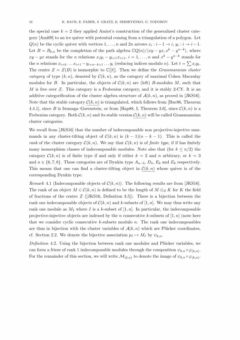
FRIEZES SATISFYING HIGHER SLk-DETERMINANTS 17
We write 0s for the images of the pI where I has a repeated entry.
As an example, we take (k, n) = (2, 5).
0 0 0 0 0 0 0 0M23 M34 M45 M15 M12 M23 M34
M13 M24 M35 M14 M25 M13 M24 · · ·· · · M14 M25 M13 M24 M35 M14 M25
M45 M15 M12 M23 M34 M45 M15 M12
0 0 0 0 0 0 0
Remark 4.3. In the finite types, the indecomposable modules are well-known. For k = 2,
they are exactly the rank 1 indecomposables. The Auslander-Reiten quivers of the cate-
gories C(3, n), for n = 6, 7, 8 are described in [JKS16]. We recall some of this information
here.
(i) For (3, 6), there are 22 indecomposable objects. Among them, 20 are rank one mod-
ules. The additional two are rank two modules filtered by M135 and M246 (in both ways).
Altogether, there are 6 projective-injective indecomposables and 16 other indecomposable
objects. The Dynkin type of C(3, 6) is D4.
(ii) For (3, 7), there are 14 rank 2 modules filtered by two rank 1 modules in addition to
the 35 rank one modules. The category C(3, 7) has 7 projective-injectives objects and is a
cluster category of type E6.
(iii) In addition to the the 56 rank one modules, C(3, 8) has 56 rank two modules and 24
rank 3 modules, all filtered by rank 1 modules. It has 8 projective-injective objects. The
Dynkin type of C(3, 8) is E8.
The categories C(3, 9) and C(4, 8) are tame, these categories are known to be of tubular
type, see [BBGE19], where the non-homogenous tubes are described.
4.2. Description of Ext-hammocks.
We determine the shape of the Ext-hammocks in M(k,n), that is, given I we describe the
set of all J appearing in the frieze M(k,n) such that Ext1C(k,n)(MI ,MJ) is nonzero. We
prove that the Ext-hammocks consist of two maximal rectangles determined by I. We
use the result in [JKS16], where the authors determine a precise combinatorial condition
for two rank 1 modules to have a nonzero extension. For this section, we allow arbitrary
1 < k < n− 1.
18 K. BAUR, E. FABER, S. GRATZ, K. SERHIYENKO, G. TODOROV
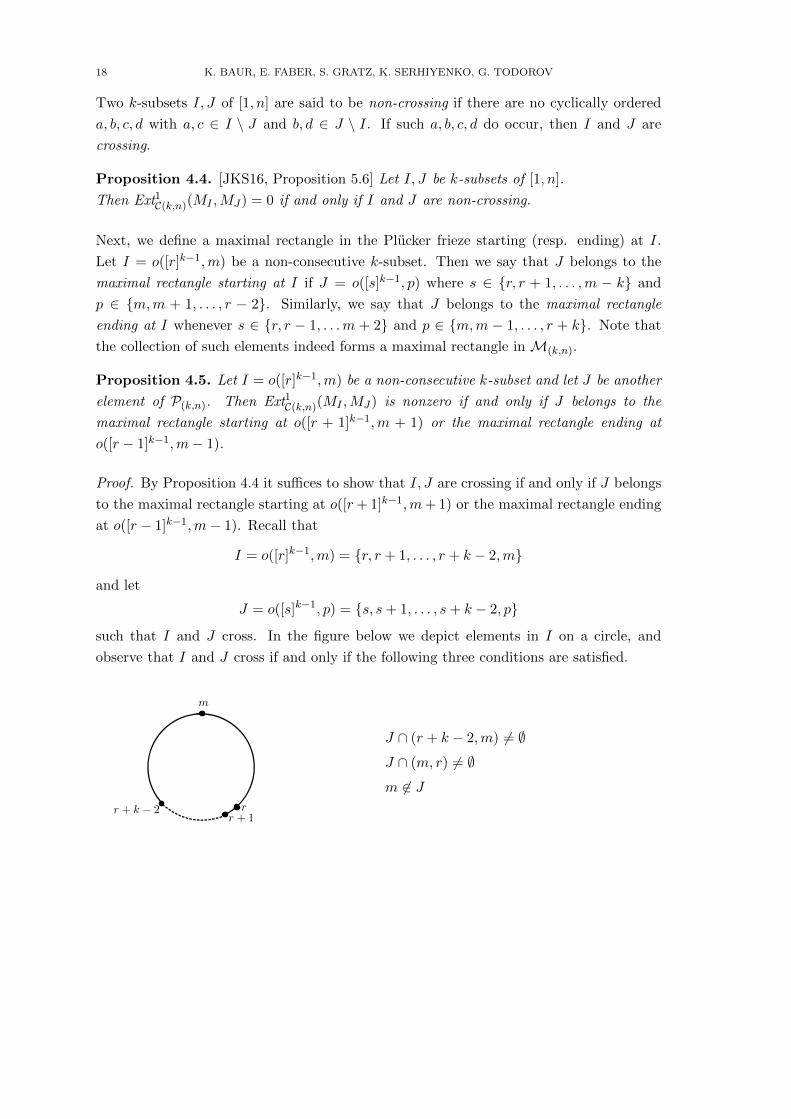
Two k-subsets I, J of [1, n] are said to be non-crossing if there are no cyclically ordered
a, b, c, d with a, c ∈ I \ J and b, d ∈ J \ I. If such a, b, c, d do occur, then I and J are
crossing.
Proposition 4.4. [JKS16, Proposition 5.6] Let I, J be k-subsets of [1, n].
Then Ext1C(k,n)(MI ,MJ) = 0 if and only if I and J are non-crossing.
Next, we define a maximal rectangle in the Plucker frieze starting (resp. ending) at I.
Let I = o([r]k−1,m) be a non-consecutive k-subset. Then we say that J belongs to the
maximal rectangle starting at I if J = o([s]k−1, p) where s ∈ {r, r + 1, . . . ,m − k} and
p ∈ {m,m + 1, . . . , r − 2}. Similarly, we say that J belongs to the maximal rectangle
ending at I whenever s ∈ {r, r − 1, . . .m + 2} and p ∈ {m,m − 1, . . . , r + k}. Note that
the collection of such elements indeed forms a maximal rectangle in M(k,n).
Proposition 4.5. Let I = o([r]k−1,m) be a non-consecutive k-subset and let J be another
element of P(k,n). Then Ext1C(k,n)(MI ,MJ) is nonzero if and only if J belongs to the
maximal rectangle starting at o([r + 1]k−1,m + 1) or the maximal rectangle ending at
o([r − 1]k−1,m− 1).
Proof. By Proposition 4.4 it suffices to show that I, J are crossing if and only if J belongs
to the maximal rectangle starting at o([r+ 1]k−1,m+ 1) or the maximal rectangle ending
at o([r − 1]k−1,m− 1). Recall that
I = o([r]k−1,m) = {r, r + 1, . . . , r + k − 2,m}
and let
J = o([s]k−1, p) = {s, s+ 1, . . . , s+ k − 2, p}
such that I and J cross. In the figure below we depict elements in I on a circle, and
observe that I and J cross if and only if the following three conditions are satisfied.
m
rr + 1
r + k − 2
J ∩ (r + k − 2,m) 6= ∅J ∩ (m, r) 6= ∅m 6∈ J

FRIEZES SATISFYING HIGHER SLk-DETERMINANTS 19
1 1 1 · · · 1 1
o([m+1]k−1,m−1) o([r+1]k−1,r−1)
o([m+1]k−1,r+k−1) o([r−1]k−1,m−1) I o([r+1]k−1,m+1) o([m−k+1]k−1,r−1)
o([r−1]k−1,r+k−1) o([m−k+1]k−1,m+1)
1 1 1 · · · 1 1
Figure 2. Ext-hammock of MI where I = o([r]k−1,m)
Note that p 6∈ [r, r + k − 2], because otherwise for the first two conditions above to be
satisfied we must have m ∈ [s]k−1 ⊂ J . This clearly contradicts the third condition.
Therefore, we have two cases p ∈ (m, r) or p ∈ (r + k − 2,m).
Suppose p ∈ (m, r). Then I and J cross if and only if s + j ∈ (r + k − 2,m) for some
j ∈ {0, 1, . . . , k − 2}, and also s+ j 6= m for any such j. This implies that s+ k − 2 < m.
On the other hand, we must also have that r < s. All together, we obtain r < s <
m − k + 2. Thus, we see from Figure 2 that J lies in the maximal rectangle starting at
o([r + 1]k−1,m+ 1).
Similarly, suppose p ∈ (r + k − 2,m). Then I and J cross if and only if s ∈ (m, r). From
Figure 2 we see that this mean J lies in the maximal rectangle ending at o([r−1]k−1,m−1).
This shows the desired claim.
�
For arbitrary k and n, the category C(k, n) contains a cluster-tilting object consisting
entirely of modules indexed by Plucker coordinates. This follows from the results in
[Sco06]. Next, we describe for which k and n there exists a cluster-tilting objected indexed
by the almost consecutive Plucker coordinates.
Proposition 4.6. A Plucker frieze of type (k, n) contains a collection I of almost consec-
utive k-element subsets such that ⊕I∈IMI is a cluster-tilting object of C(k, n) if and only
if k = 2, 3 with n arbitrary, or k = 4 and n = 6.
Proof. In general, the cluster category C(k, n) contains a cluster-tilting object consisting of
(k− 1)(n− k− 1) indecomposable summands. Therefore, we want to show that a Plucker
frieze contains (k− 1)(n− k− 1) distinct k-element subsets that are pairwise non-crossing
if and only if k = 2, 3 or k = 4 and n = 6.
20 K. BAUR, E. FABER, S. GRATZ, K. SERHIYENKO, G. TODOROV
If k = 2 then every object in C(k, n) is of the form MI where I is a 2 element subset of
[1, n]. In particular, every such I lies in the associated Plucker frieze. This shows the
claim for k = 2.
If k = 3 we want to find 2(n − 4) pairwise non-crossing elements in the Plucker frieze.
Consider the following collection of 3-element subsets of [1, n] consisting of two disjoint
families of size n− 4.
{1, 2,m}m=4,5,...,n−1 and {s, s+ 1, 1}s=3,4,...,n−2
Each of these corresponds to a diagonal in the Plucker frieze, thus by Proposition 4.5 we
see that no two elements in the same family cross. Moreover, {1, 2,m} does not cross
{s, s + 1, 1} by definition. This shows that the collection of 3-element subsets above are
pairwise non-crossing.
If k ≥ 4 we want to show that the associated Plucker frieze does not contain (k−1)(n−k−1)
pairwise non-crossing elements unless k = 4 and n = 6. We make use of the following
key observation here: the Ext-hammocks in a frieze of width w have the same shape as
the Ext-hammocks in the cluster category of type A with rank w. In particular, any
region in the frieze that has the same shape as the fundamental region in the associated
cluster category of type A, as depicted on the left in Figure 3, contains at most w pairwise
non-crossing objects.
First we consider the case k = 4 separately. We see that the Plucker frieze admits two
copies of the fundamental region followed by two columns, because we have w = n−k−1 =
n− 5 and the period of the frieze is n. See Figure 3 on the right. Now suppose that such
frieze admits a collection I of 3w pairwise non-crossing objects. Because the frieze contains
two such fundamental regions, each of which admits at most w non-crossing object, we
conclude that the two remaining columns contain at least w element of I. However, a
frieze is n-periodic, and the same argument as above implies that any two neighbouring
columns contain at least w elements of I. Because there are w + 5 columns we conclude
that I contains at least ⌊w + 5
2
⌋w
elements. We also know that the size of I is 3w which implies that⌊w+52
⌋≤ 3. Therefore,
there are two possibilities w = 1, k = 4, n = 6 or w = 2, k = 4, n = 7. In the first case, we
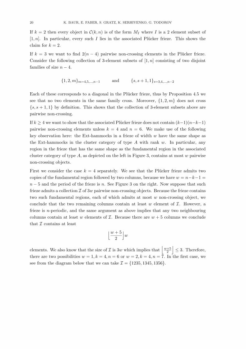
see from the diagram below that we can take I = {1235, 1345, 1356}.
FRIEZES SATISFYING HIGHER SLk-DETERMINANTS 21
1 1 1 1 1 1 1 1
1235 2346 1345 2456 1356 1246 1235
1 1 1 1 1 1 1 1
In the second case, one can check that it is not possible to find I of size 6. This completes
the proof for k = 4.
Finally, suppose k > 4 and let I be a collection of pairwise non-crossing elements in the
Plucker frieze of size (k − 1)(n − k − 1) = (k − 1)w. By the same reasoning as in the
previous case we think of subdividing the frieze into fundamental regions. We begin by
taking two copies of the frieze, so we have a rectangular array of elements of width w and
length 2n. Next, we want to subdivide it into rectangles of width w and length w + 3,
see Figure 3 on the right. Moreover, each such rectangular region contains at most 2w
elements of I. But in the beginning we took two copies of the frieze, so dividing by two,
we see that a Plucker frieze contains at most⌈ 2n
w + 3
⌉w
pairwise non-crossing elements. To prove the claim it suffices to show that
(k − 1)w >⌈ 2n
w + 3
⌉w
Below, we will show that
(5) k − 1 >2n
w + 3+ 1
holds, which in turn implies the equation above. Multiplying equation (5) by w + 3 and
substituting w + 3 = n− k + 2 we obtain
(6) (k − 4)n > (k − 2)2
Since k > 4 we can write
n > k − 2 >(k − 2)(k − 2)
k − 4which in turn implies equations (6) and (5). This completes the proof in the case k > 4.
�
In terms of cluster algebras we get the following:
Corollary 4.7. A Plucker frieze of type (k, n) contains a collection I of almost consecutive
k-element subsets such that the collection {pI | I ∈ I} is a cluster in sA(k, n) if and only
if k = 2, 3 with n arbitrary or k = 4 and n = 6.
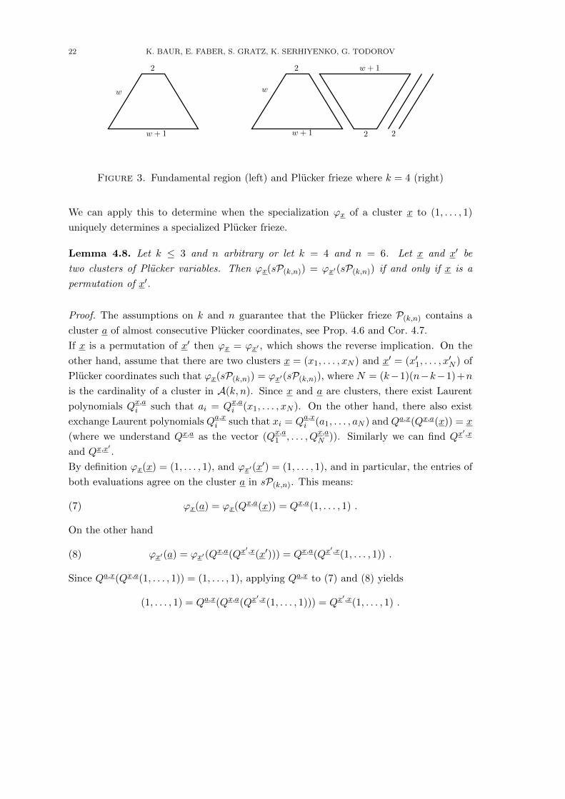
22 K. BAUR, E. FABER, S. GRATZ, K. SERHIYENKO, G. TODOROV
2
w
w + 1
2 2
2w + 1
w + 1
w
Figure 3. Fundamental region (left) and Plucker frieze where k = 4 (right)
We can apply this to determine when the specialization ϕx of a cluster x to (1, . . . , 1)
uniquely determines a specialized Plucker frieze.
Lemma 4.8. Let k ≤ 3 and n arbitrary or let k = 4 and n = 6. Let x and x′ be
two clusters of Plucker variables. Then ϕx(sP(k,n)) = ϕx′(sP(k,n)) if and only if x is a
permutation of x′.
Proof. The assumptions on k and n guarantee that the Plucker frieze P(k,n) contains a
cluster a of almost consecutive Plucker coordinates, see Prop. 4.6 and Cor. 4.7.
If x is a permutation of x′ then ϕx = ϕx′ , which shows the reverse implication. On the
other hand, assume that there are two clusters x = (x1, . . . , xN ) and x′ = (x′1, . . . , x′N ) of
Plucker coordinates such that ϕx(sP(k,n)) = ϕx′(sP(k,n)), where N = (k−1)(n−k−1)+n
is the cardinality of a cluster in A(k, n). Since x and a are clusters, there exist Laurent
polynomials Qx,ai such that ai = Q
x,ai (x1, . . . , xN ). On the other hand, there also exist
exchange Laurent polynomials Qa,xi such that xi = Q
a,xi (a1, . . . , aN ) and Qa,x(Qx,a(x)) = x
(where we understand Qx,a as the vector (Qx,a1 , . . . , Q
x,aN )). Similarly we can find Qx′,x
and Qx,x′ .
By definition ϕx(x) = (1, . . . , 1), and ϕx′(x′) = (1, . . . , 1), and in particular, the entries of
both evaluations agree on the cluster a in sP(k,n). This means:
(7) ϕx(a) = ϕx(Qx,a(x)) = Qx,a(1, . . . , 1) .
On the other hand
(8) ϕx′(a) = ϕx′(Qx,a(Qx′,x(x′))) = Qx,a(Qx′,x(1, . . . , 1)) .
Since Qa,x(Qx,a(1, . . . , 1)) = (1, . . . , 1), applying Qa,x to (7) and (8) yields
(1, . . . , 1) = Qa,x(Qx,a(Qx′,x(1, . . . , 1))) = Qx′,x(1, . . . , 1) .

FRIEZES SATISFYING HIGHER SLk-DETERMINANTS 23
Note that, while we have defined the cluster algebra A(k, n) as a C-algebra, we have in
fact
A(k, n) = C⊗C AZ(k, n),
whereAZ(k, n) is a cluster algebra of geometric type, defined as the subring of Q(x1, . . . , xN )
generated by the cluster variables. Assume now as a contradiction that x is not a permu-
tation of x′. Then there is an 1 ≤ i ≤ N such that xi /∈ {x′1, . . . , x′N} and
xi = Qx′,xi (x′1, . . . , x
′N ) =
f(x′1, . . . , x′N )
x′d11 · · ·x′dNN
,
with x′j - f(x′) for all 1 ≤ j ≤ N . By positivity [GHKK18, LS15] this is a Laurent
polynomial over Z≥0. Therefore, Qx′,xi (x′1, . . . , x
′N ) = 1 implies that f is the constant
polynomial f = 1 and
xi =1
x′d11 · · ·x′dNN
.
However, by positivity of d-vectors, which was shown for skew-symmetric cluster algebras
by [CL17, Thm. 1.2], we have dj ≥ 0 for all 1 ≤ j ≤ N and so xi is a unit in AZ(k, n);
contradicting [GLS13, Theorem 1.3]. �
4.3. Mesh friezes.
Assume k ≤ n/2. We recall that the Grassmannian cluster category C(k, n) is of finite
type if and only if either k = 2, or k = 3 and n ∈ {6, 7, 8} (Section 4.1).
Definition 4.9. Let C(k, n) be of finite type. A mesh frieze Fk,n for the Grassmannian
cluster category C(k, n) is a collection of positive integers, one for each indecomposable
object in C(k, n) such the Fk,n(P ) = 1 for every indecomposable projective-injective P
and such that all mesh relations on the AR-quiver of C(k, n) evaluate to 1 thus, whenever
we have an AR-sequence
(9) 0→ A→I⊕
i=1
Bi → C → 0,
where the Bi are indecomposable, and I ≥ 1, we get
Fk,n(A)Fk,n(C) =I∏
i=1
Fk,n(Bi) + 1.
(Note that C(k, n) has Auslander-Reiten sequences and an Auslander-Reiten quiver, cf.
for example [JKS16, Remark 3.3 ].)

24 K. BAUR, E. FABER, S. GRATZ, K. SERHIYENKO, G. TODOROV
Example 4.10. In case k = 2, a mesh frieze F2,n for C(2, n) is an integral frieze pattern (or
an integral SL2-frieze). In that case, the notion of mesh friezes and of integral SL2-friezes
coincide. Such friezes are in bijection with triangulations of an n-gon and hence arise from
specialising a cluster to 1, see Example 2.4.
Remark 4.11. Note that [ARS10] introduce the notion of ‘friezes of Dynkin type’. It
coincides with certain mesh friezes (on the stable version C(k, n)) in types An, D4, E6, E8.
Remark 4.12. Recall that C(k, n) is a categorification of the cluster algebra A(k, n). Fur-
thermore, the mesh frieze has 1’s at the projective-injective objects, i.e., the objects for
consecutive k-subsets. In that sense, any mesh frieze Fk,n for C(k, n) is also a mesh frieze
associated to the cluster algebra sA(k, n) = A(k, n)/J with coefficients specialized to 1,
cf. Remark 2.8. The requirement that mesh relations evaluate to 1 translates to requiring
that certain exchange relations in the cluster algebra hold. We will use both points of
view. The approach to friezes via C(k, n) is particularly useful when we want to check
for the existence of cluster-tilting objects in the SLk-frieze. It will also be of importance
in Section 5 as we want to use Iyama–Yoshino reductions on these categories to analyse
frieze patterns.
Remark 4.13. Note that the entries in a mesh frieze satisfy the exchange relations of the
associated cluster algebra A(k, n). That is, denoting by xN the cluster variable in A(k, n)
associated to an indecomposable object N in C(k, n) the following holds: Whenever we
have an exchange relation
xAxC =
m∏i=1
xBi+
m′∏j=1
xB′j
in A(k, n), then
F(A)F(B) =m∏i=1
F(Bi) +m′∏j=1
F(B′j).
Indeed, this follows from the fact that a mesh frieze is determined uniquely by the values of
one cluster tilting object. Thus, we may take an acyclic cluster that forms a slice because
k = 2 and n is arbitrary or k = 3 and n = 6, 7, 8, and then use sink/source mutations
to determine all entries in the mesh frieze uniquely. Now this exact same cluster also
determines values on the mesh frieze uniquely using arbitrary mutations of the cluster
algebra. Thus, these two approaches should yield the exact same mesh frieze, which
implies that the entries in the mesh frieze satisfy all relations of the cluster algebra, not
just the ones coming from sink/source mutations.
FRIEZES SATISFYING HIGHER SLk-DETERMINANTS 25
4.4. Mesh friezes for C(k, n) yield SLk-friezes.
In this section, we show the correspondence between integral tame SLk-friezes and mesh
friezes in the finite type cases. For k = 2, these two notions coincide (see Example 4.10).
So for the rest of this section, we assume k = 3 and n ∈ {6, 7, 8}. The width of such an
SL3-frieze is n− 4, see Remark 2.3.
The following lemma shows that the entries in a tame SL3-frieze are determined by a
cluster of A(k, n), which consists of consecutive Plucker coordinates.
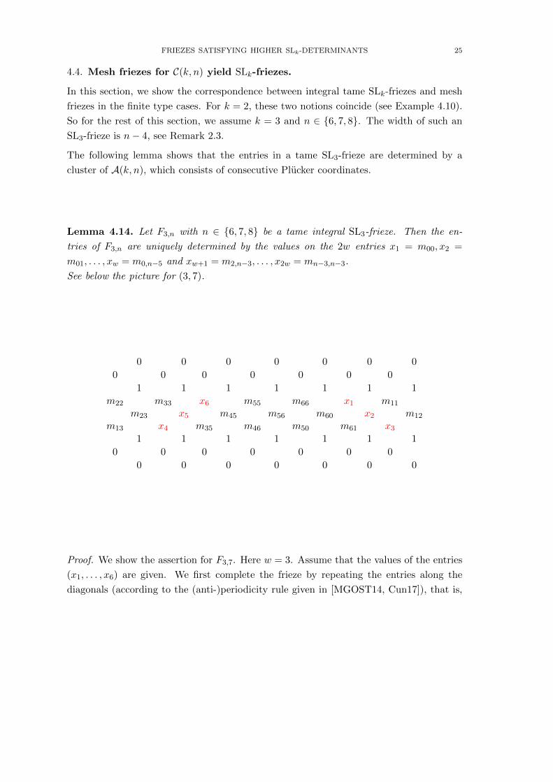
Lemma 4.14. Let F3,n with n ∈ {6, 7, 8} be a tame integral SL3-frieze. Then the en-
tries of F3,n are uniquely determined by the values on the 2w entries x1 = m00, x2 =
m01, . . . , xw = m0,n−5 and xw+1 = m2,n−3, . . . , x2w = mn−3,n−3.
See below the picture for (3, 7).
0 0 0 0 0 0 0
0 0 0 0 0 0 0
1 1 1 1 1 1 1
m22 m33 x6 m55 m66 x1 m11
m23 x5 m45 m56 m60 x2 m12
m13 x4 m35 m46 m50 m61 x31 1 1 1 1 1 1
0 0 0 0 0 0 0
0 0 0 0 0 0 0
Proof. We show the assertion for F3,7. Here w = 3. Assume that the values of the entries
(x1, . . . , x6) are given. We first complete the frieze by repeating the entries along the
diagonals (according to the (anti-)periodicity rule given in [MGOST14, Cun17]), that is,
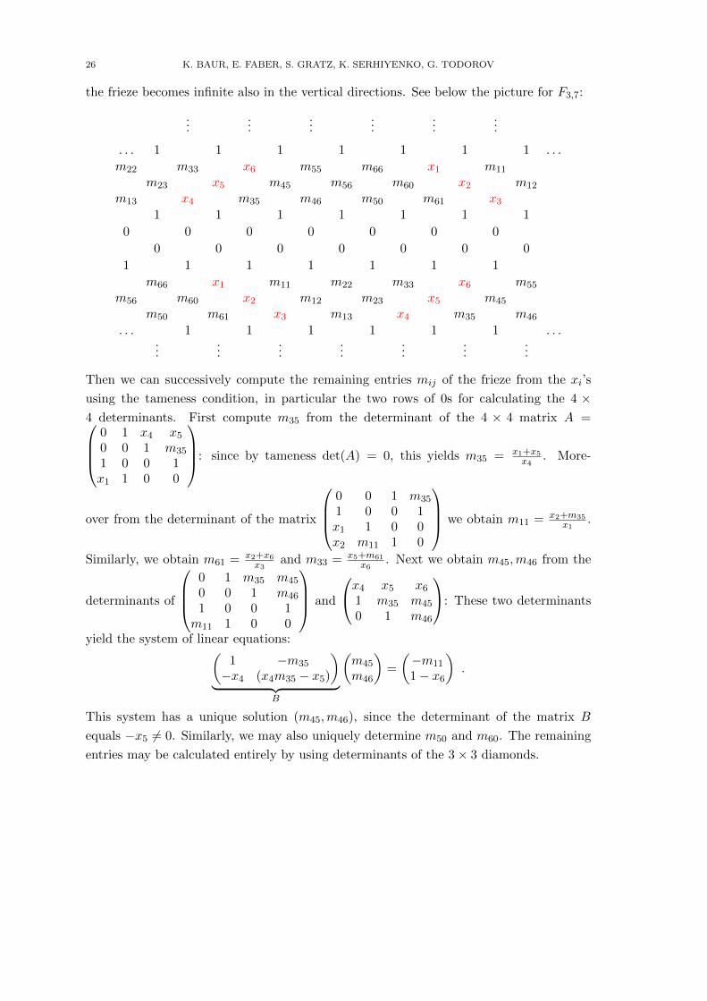
26 K. BAUR, E. FABER, S. GRATZ, K. SERHIYENKO, G. TODOROV
the frieze becomes infinite also in the vertical directions. See below the picture for F3,7:
......
......
......
. . . 1 1 1 1 1 1 1 . . .
m22 m33 x6 m55 m66 x1 m11
m23 x5 m45 m56 m60 x2 m12
m13 x4 m35 m46 m50 m61 x31 1 1 1 1 1 1
0 0 0 0 0 0 0
0 0 0 0 0 0 0
1 1 1 1 1 1 1
m66 x1 m11 m22 m33 x6 m55
m56 m60 x2 m12 m23 x5 m45
m50 m61 x3 m13 x4 m35 m46
. . . 1 1 1 1 1 1 . . ....
......
......
......
Then we can successively compute the remaining entries mij of the frieze from the xi’s
using the tameness condition, in particular the two rows of 0s for calculating the 4 ×4 determinants. First compute m35 from the determinant of the 4 × 4 matrix A =
0 1 x4 x50 0 1 m35
1 0 0 1x1 1 0 0
: since by tameness det(A) = 0, this yields m35 = x1+x5x4
. More-
over from the determinant of the matrix
0 0 1 m35
1 0 0 1x1 1 0 0x2 m11 1 0
we obtain m11 = x2+m35x1
.
Similarly, we obtain m61 = x2+x6x3
and m33 = x5+m61x6
. Next we obtain m45,m46 from the
determinants of
0 1 m35 m45
0 0 1 m46
1 0 0 1m11 1 0 0
and
x4 x5 x61 m35 m45
0 1 m46
: These two determinants
yield the system of linear equations:(1 −m35
−x4 (x4m35 − x5)
)︸ ︷︷ ︸
B
(m45
m46
)=
(−m11
1− x6
).
This system has a unique solution (m45,m46), since the determinant of the matrix B
equals −x5 6= 0. Similarly, we may also uniquely determine m50 and m60. The remaining
entries may be calculated entirely by using determinants of the 3× 3 diamonds.
FRIEZES SATISFYING HIGHER SLk-DETERMINANTS 27
The assertion for the cases (3, 6) and (3, 8) are proven by analogous tedious calculations.
�
Proposition 4.15. Let w ∈ {2, 3, 4} and n = w + 4. For every tame integral SL3-frieze
of width w there exists a mesh frieze on C(3, n).
Proof. Let F = F3,n be a SL3-frieze of horizontal period n = w + 4, for w ∈ {2, 3, 4}.Consider the Plucker frieze P(k, n) of type (3, n). It has the same width and period as
F , and we can overlay P(k, n) on top of F such that every pI for an almost consecutive
3-subset I of [1, n] comes to lie on top of an entry in F . (Note that a choice is involved
here, the way to overlay F by P(k, n) is not unique.) This assigns to each entry pI in
the Plucker frieze P(k, n) an integer f(pI) lying underneath pI . By Proposition 4.6, the
Plucker frieze P(k, n) contains a collection of entries {pI | I ∈ I} such that⊕
I∈IMI is
a cluster-tilting object of C(3, n). Its image under ψ−13,n is a cluster in A(3, n) (cf. Corol-
lary 4.7). Specializing the indecomposable object MI for I ∈ I to f(pI) and calculating
the remaining entries using the mesh relations yields a mesh frieze on the AR-quiver of
C(3, n): By construction, the mesh relations are satisfied and as explained in Remark 3.10
all its entries are positive rationals. It remains to show that the entries are all integers.
For this, we associate positive integers from F to their positions in the corresponding
Auslander-Reiten quiver/mesh frieze and use the mesh relations to see that all the other
entries are sums and differences of products of these given positive integers. That proves
the claim. We include pictures of the Auslander-Reiten quivers of these three categories
along the way.
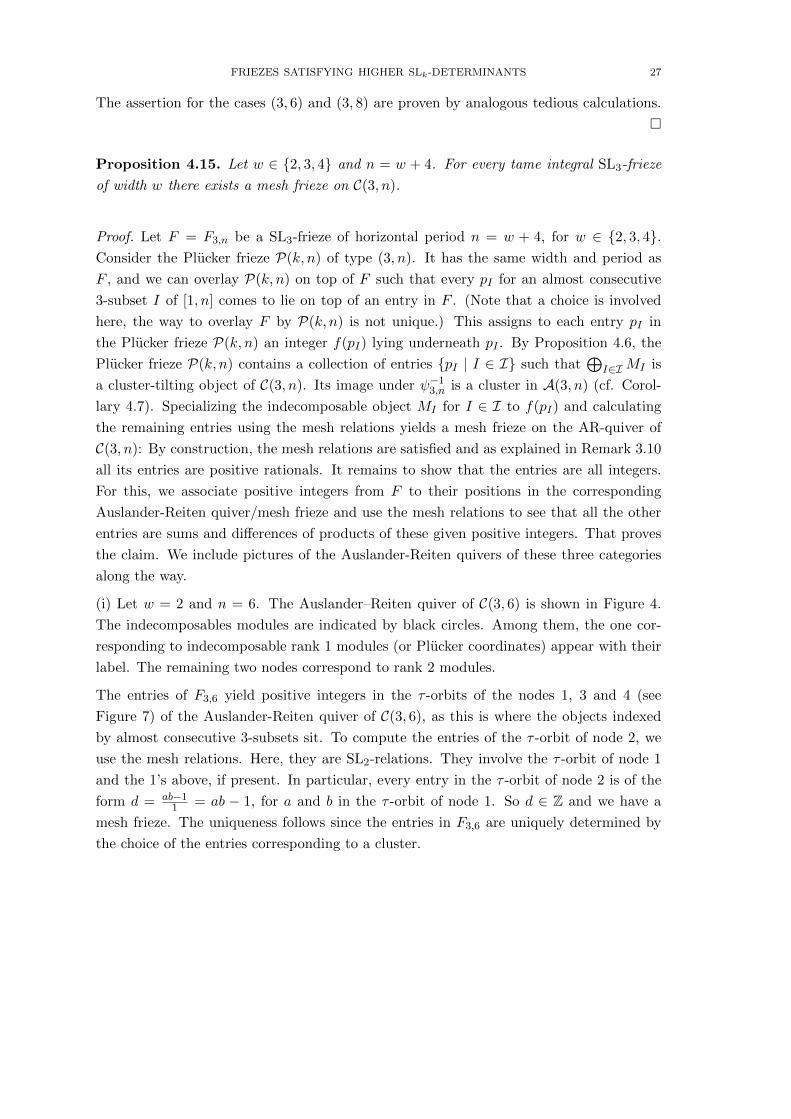
(i) Let w = 2 and n = 6. The Auslander–Reiten quiver of C(3, 6) is shown in Figure 4.
The indecomposables modules are indicated by black circles. Among them, the one cor-
responding to indecomposable rank 1 modules (or Plucker coordinates) appear with their
label. The remaining two nodes correspond to rank 2 modules.
The entries of F3,6 yield positive integers in the τ -orbits of the nodes 1, 3 and 4 (see
Figure 7) of the Auslander-Reiten quiver of C(3, 6), as this is where the objects indexed
by almost consecutive 3-subsets sit. To compute the entries of the τ -orbit of node 2, we
use the mesh relations. Here, they are SL2-relations. They involve the τ -orbit of node 1
and the 1’s above, if present. In particular, every entry in the τ -orbit of node 2 is of the
form d = ab−11 = ab − 1, for a and b in the τ -orbit of node 1. So d ∈ Z and we have a
mesh frieze. The uniqueness follows since the entries in F3,6 are uniquely determined by
the choice of the entries corresponding to a cluster.
28 K. BAUR, E. FABER, S. GRATZ, K. SERHIYENKO, G. TODOROV
123
126 345
125
456
256 134235134 146
125 136 245 346
246135
356 145 236 124
234 156
356
Figure 4. Auslander-Reiten quiver of C(3, 6). Projective-injectives aredrawn as white circles.
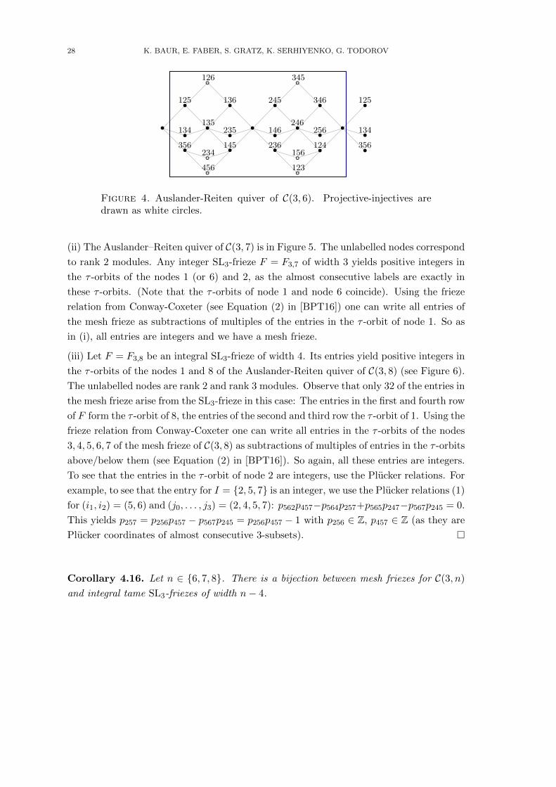
(ii) The Auslander–Reiten quiver of C(3, 7) is in Figure 5. The unlabelled nodes correspond
to rank 2 modules. Any integer SL3-frieze F = F3,7 of width 3 yields positive integers in
the τ -orbits of the nodes 1 (or 6) and 2, as the almost consecutive labels are exactly in
these τ -orbits. (Note that the τ -orbits of node 1 and node 6 coincide). Using the frieze
relation from Conway-Coxeter (see Equation (2) in [BPT16]) one can write all entries of
the mesh frieze as subtractions of multiples of the entries in the τ -orbit of node 1. So as
in (i), all entries are integers and we have a mesh frieze.
(iii) Let F = F3,8 be an integral SL3-frieze of width 4. Its entries yield positive integers in
the τ -orbits of the nodes 1 and 8 of the Auslander-Reiten quiver of C(3, 8) (see Figure 6).
The unlabelled nodes are rank 2 and rank 3 modules. Observe that only 32 of the entries in
the mesh frieze arise from the SL3-frieze in this case: The entries in the first and fourth row
of F form the τ -orbit of 8, the entries of the second and third row the τ -orbit of 1. Using the
frieze relation from Conway-Coxeter one can write all entries in the τ -orbits of the nodes
3, 4, 5, 6, 7 of the mesh frieze of C(3, 8) as subtractions of multiples of entries in the τ -orbits
above/below them (see Equation (2) in [BPT16]). So again, all these entries are integers.
To see that the entries in the τ -orbit of node 2 are integers, use the Plucker relations. For
example, to see that the entry for I = {2, 5, 7} is an integer, we use the Plucker relations (1)
for (i1, i2) = (5, 6) and (j0, . . . , j3) = (2, 4, 5, 7): p562p457−p564p257+p565p247−p567p245 = 0.
This yields p257 = p256p457 − p567p245 = p256p457 − 1 with p256 ∈ Z, p457 ∈ Z (as they are
Plucker coordinates of almost consecutive 3-subsets). �
Corollary 4.16. Let n ∈ {6, 7, 8}. There is a bijection between mesh friezes for C(3, n)
and integral tame SL3-friezes of width n− 4.
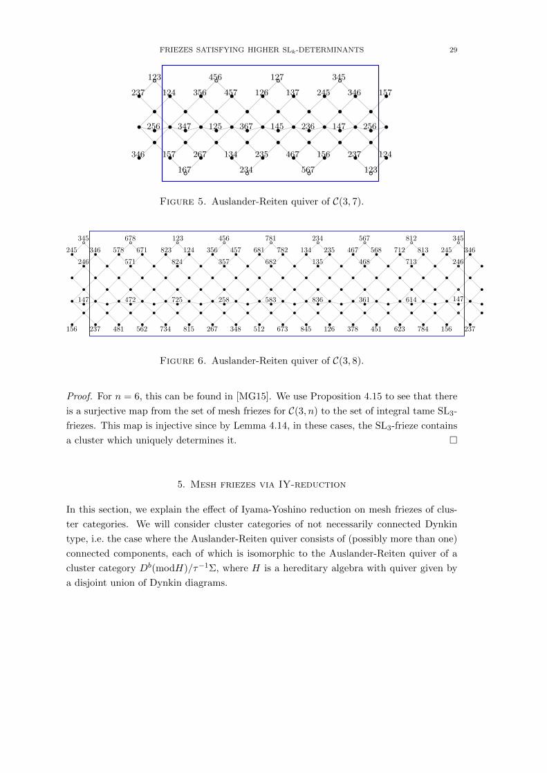
FRIEZES SATISFYING HIGHER SLk-DETERMINANTS 29
267 235 156157 237
167
123 456 127 345
234 567 123
245124237 356 457 126 137 346
346 134 467
157
125 145 147367 236 256256 347
124
Figure 5. Auslander-Reiten quiver of C(3, 7).
345
245 346 578 823 356 681 134 467 712 245
678 123 456 781 234 567 812
671 124 457 782 235 568 813
246 571 824 357 682 135 468 713 246
345
147
237156 156
147
481 734 267 512 845 378 623562 815 348 673 126 451 784
472 725 258 583 836 361 614
346
237
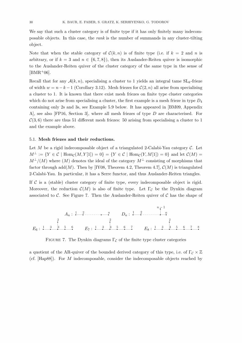
Figure 6. Auslander-Reiten quiver of C(3, 8).
Proof. For n = 6, this can be found in [MG15]. We use Proposition 4.15 to see that there
is a surjective map from the set of mesh friezes for C(3, n) to the set of integral tame SL3-
friezes. This map is injective since by Lemma 4.14, in these cases, the SL3-frieze contains
a cluster which uniquely determines it. �
5. Mesh friezes via IY-reduction
In this section, we explain the effect of Iyama-Yoshino reduction on mesh friezes of clus-
ter categories. We will consider cluster categories of not necessarily connected Dynkin
type, i.e. the case where the Auslander-Reiten quiver consists of (possibly more than one)
connected components, each of which is isomorphic to the Auslander-Reiten quiver of a
cluster category Db(modH)/τ−1Σ, where H is a hereditary algebra with quiver given by
a disjoint union of Dynkin diagrams.
30 K. BAUR, E. FABER, S. GRATZ, K. SERHIYENKO, G. TODOROV
We say that such a cluster category is of finite type if it has only finitely many indecom-
posable objects. In this case, the rank is the number of summands in any cluster-tilting
object.
Note that when the stable category of C(k, n) is of finite type (i.e. if k = 2 and n is
arbitrary, or if k = 3 and n ∈ {6, 7, 8}), then its Auslander-Reiten quiver is isomorphic
to the Auslander-Reiten quiver of the cluster category of the same type in the sense of
[BMR+06].
Recall that for any A(k, n), specialising a cluster to 1 yields an integral tame SLk-frieze
of width w = n−k− 1 (Corollary 3.12). Mesh friezes for C(2, n) all arise from specialising
a cluster to 1. It is known that there exist mesh friezes on finite type cluster categories
which do not arise from specialising a cluster, the first example is a mesh frieze in type D4
containing only 2s and 3s, see Example 5.9 below. It has appeared in [BM09, Appendix
A], see also [FP16, Section 3], where all mesh friezes of type D are characterised. For
C(3, 6) there are thus 51 different mesh friezes: 50 arising from specialising a cluster to 1
and the example above.
5.1. Mesh friezes and their reductions.
Let M be a rigid indecomposable object of a triangulated 2-Calabi-Yau category C. Let
M⊥ := {Y ∈ C | HomC(M,Y [1]) = 0} = {Y ∈ C | HomC(Y,M [1]) = 0} and let C(M) =
M⊥/(M) where (M) denotes the ideal of the category M⊥ consisting of morphisms that
factor through add(M). Then by [IY08, Theorem 4.2, Theorem 4.7], C(M) is triangulated
2-Calabi-Yau. In particular, it has a Serre functor, and thus Auslander-Reiten triangles.
If C is a (stable) cluster category of finite type, every indecomposable object is rigid.
Moreover, the reduction C(M) is also of finite type. Let ΓC be the Dynkin diagram
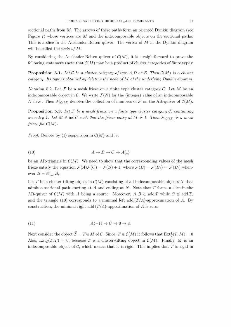
associated to C. See Figure 7. Then the Auslander-Reiten quiver of C has the shape of
An : 1 2 n Dn : 1 2 n
n− 1
E6 : 1 3 4 5 6
2
E7 : 1 3 4 5 6
2
7 E8 : 1 3 4 5 6
2
7 8
Figure 7. The Dynkin diagrams ΓC of the finite type cluster categories
a quotient of the AR-quiver of the bounded derived category of this type, i.e. of ΓC × Z(cf. [Hap88]). For M indecomposable, consider the indecomposable objects reached by
FRIEZES SATISFYING HIGHER SLk-DETERMINANTS 31
sectional paths from M . The arrows of these paths form an oriented Dynkin diagram (see
Figure 7) whose vertices are M and the indecomposable objects on the sectional paths.
This is a slice in the Auslander-Reiten quiver. The vertex of M in the Dynkin diagram
will be called the node of M .
By considering the Auslander-Reiten quiver of C(M), it is straightforward to prove the
following statement (note that C(M) may be a product of cluster categories of finite type):
Proposition 5.1. Let C be a cluster category of type A,D or E. Then C(M) is a cluster
category. Its type is obtained by deleting the node of M of the underlying Dynkin diagram.
Notation 5.2. Let F be a mesh frieze on a finite type cluster category C. Let M be an
indecomposable object in C. We write F(N) for the (integer) value of an indecomposable
N in F . Then F|C(M) denotes the collection of numbers of F on the AR-quiver of C(M).
Proposition 5.3. Let F be a mesh frieze on a finite type cluster category C, containing
an entry 1. Let M ∈ ind C such that the frieze entry at M is 1. Then F|C(M) is a mesh
frieze for C(M).
Proof. Denote by 〈1〉 suspension in C(M) and let
(10) A→ B → C → A〈1〉
be an AR-triangle in C(M). We need to show that the corresponding values of the mesh
frieze satisfy the equation F(A)F(C) = F(B) + 1, where F(B) = F(B1) · · · F(Bt) when-
ever B = ⊕ti=1Bi.
Let T be a cluster tilting object in C(M) consisting of all indecomposable objects N that
admit a sectional path starting at A and ending at N . Note that T forms a slice in the
AR-quiver of C(M) with A being a source. Moreover, A,B ∈ addT while C 6∈ addT ,
and the triangle (10) corresponds to a minimal left add (T/A)-approximation of A. By
construction, the minimal right add (T/A)-approximation of A is zero.
(11) A〈−1〉 → C → 0→ A
Next consider the object T = T ⊕M of C. Since, T ∈ C(M) it follows that Ext1C(T,M) = 0
Also, Ext1C(T, T ) = 0, because T is a cluster-tilting object in C(M). Finally, M is an
indecomposable object of C, which means that it is rigid. This implies that T is rigid in
32 K. BAUR, E. FABER, S. GRATZ, K. SERHIYENKO, G. TODOROV
C. Thus, T is a cluster-tilting object in C as it has the correct number of indecomposable
summands.
The AR-triangles (10) and (11) in C(M) lift to the corresponding triangles in C:
(12) A→ B → C → A[1] A[−1]→ C → B′ → A
where B ∼= B ⊕ M i and B′ ∼= M j for some non-negative integers i, j and [1] denotes
suspension in C. Here, M0 denotes the zero module. Moreover, we see that the two
triangles in (12) are the left and right add T /A-approximations of A respectively.
Let A be the cluster algebra associated to C. For an object N ∈ C let xN denote the
associated (product of) cluster variable(s) in A. Because C is the categorification of Ait follows that the two triangles (12) give rise to the following exchange relation in the
cluster algebra.
xAxC = xB
+ xB′
Note that the entries of the associated mesh frieze F also satisfy the relations of the cluster
algebra A. By Remark 4.13 we obtain the desired equation
F(A)F(C) = F(B) + F(B′) = F(B)F(M i) + F(M j) = F(B) + 1
because F(M1) = F(M) = 1 and F(M0) = F(0) = 1. �
Remark 5.4. We can use Proposition 5.3 to argue that a mesh frieze for C always has ≤ mentries 1, if m is the rank of C: Let F be a mesh frieze for C, a cluster category of rank
m. Assume that F has > m entries 1. Take M0 indecomposable such that its entry in the
frieze is 1. Let C1 := C(M0). This has rank m− 1. Let F1 = F |C1 . Take M1 ∈ ind C1 such
that the entry of M1 in F1 is 1. Let C2 := C1(M1). This is a cluster category of rank m−2
and F2 := F1 |C2 has ≥ m−1 entries equal to 1. Iterate until the resulting cluster category
is a product of cluster categories of type A, whose rank is m′ (and m′ ≥ 3) and where
the associated frieze F ′ has ≥ m′ + 1 entries equal to 1s. Contradiction. Here, we also
might need to justify that passing from F to F1 we loose exactly one entry in the frieze
that equals 1. This holds, because suppose on the contrary that F(M0) = F(M ′0) = 1,
where M ′0 is some other indecomposable object of C, and M ′0 6∈ M⊥0 . This implies that
Ext1C(M0,M′0) 6= 0. In particular, there exist two triangles in C
M0 → B →M ′0 →M0[1] M ′0 → B′ →M0 →M ′0[1].
FRIEZES SATISFYING HIGHER SLk-DETERMINANTS 33
And by the same reasoning as in the proof of the above proposition, we obtain
F(M0)F(M ′0) = F(B) + F(B′).
The right hand side is clearly ≥ 2, because F is an integral mesh frieze. This is a contra-
diction to F(M0) = F(M ′0) = 1.
5.2. Counting friezes.
In this section, we study the number of mesh friezes for the Grassmannian cluster categories
C(3, n) in the finite types (types D4, E6 and E8) and for the cluster category of type E7.
We recover the known number of mesh friezes for C(3, 7) and find all the known mesh
friezes for C(3, 8) and for cluster categories of type E7. Recall that specialising a cluster
to 1 gives a unique mesh frieze on C(k, n), cf. Corollary 3.12.
Definition 5.5. A unitary mesh frieze is a mesh frieze which arises from specialising a
cluster to 1.
Not every frieze pattern arises this way. Some mesh friezes have less 1’s than the rank of
the cluster category. These are called non-unitary friezes. We will focus on these in what
follows.
Remark 5.6. For k = 2, the notion of mesh frieze coincides with the notion of SL2-frieze
and the numbers of them are well-known, they are counted by the Catalan numbers. In
particular, they all arise from specialising a cluster to 1. From now on, we thus concentrate
on k = 3 and n ∈ {6, 7, 8}. Recall first that the case (3, 6) corresponds to a cluster
category of type D4, the case (3, 7) to a cluster category of type E6 and the case (3,8) to a
cluster category of type E8. The number of clusters in these types are 50, 833 and 25080
respectively, see e.g. [FZ03, Table 3].
It is known that the number of SL3-friezes of width 2 or, equivalently, the number of mesh
friezes for C(3, 6) is 51 (this is proven via 2-friezes in [MGOT12, Prop. 6.2], and can be
checked using a computer algebra system or counting the mesh friezes on a cluster category
of type D4, see Example 5.9 below). The number of SL3-friezes (equivalently, the number
of mesh friezes for C(3, 7)) of width 3 is 868 by Theorem B.1. Note that this number was
already stated, citing a private communication by Cuntz, in [MG15]. Appendix B now
provides a proof for this statement
Fontaine and Plamondon found 26952 mesh friezes for C(3, 8), see the lists on [FP], see
also [Cun17, Conjecture 2.1] and [MG15, Section 4.4].

34 K. BAUR, E. FABER, S. GRATZ, K. SERHIYENKO, G. TODOROV
We also recall that the number of clusters in a cluster category of type E7 is 4160. Con-
jecturally, there are 4400 mesh friezes in type E7 ([FP]).
Corollary 5.7. Let F be a mesh frieze on a finite type cluster category C and M ∈ ind Can object whose frieze entry is 1. Then the following holds:
(1) If F ′ := F|C(M) is unitary, then F is unitary.
(2) If the Dynkin type of C(M) is A or a product of A-types, then F is unitary.
Proof. Let n be the rank of C. By Proposition 5.3, F ′ := F|C(M) is a mesh frieze for C(M).
If C(M) is unitary, then F ′ contains n − 1 entries equal to 1. But then F contains n 1s
and is unitary. The second statement then follows, since in type A, all mesh friezes are
unitary. �
An immediate consequence of Corollary 5.7 is the following.
Corollary 5.8. Let F be a mesh frieze on a cluster category of type D or E. If F contains
an entry 1 at the branch node or at a node which is an immediate neighbour of the branch
node, then F is unitary.
By Corollary 5.8, non-unitary friezes cannot exist in ranks ≤ 3: In terms of ranks, the
smallest possible cluster category with non-unitary mesh friezes is of type D4. Indeed, we
have one in this case, see Example 5.9.
Example 5.9. There exists a non-unitary mesh frieze in type D4 ([BM09, Appendix A]. It
is the only non-unitary mesh frieze in type D4, see [FP16, Section 3]).
2 2 2 2
3 3 3 3
· · · 2 2 2 2 · · ·2 2 2 2
5.2.1. Non-unitary mesh friezes in type E6. Let C be a cluster category of type E6. Using
the result of Cuntz and Plamondon (B.1), one can deduce that there are 35 non-unitary
mesh friezes for C. One can extract these from the lists available on [FP]. One can check
that each of them contains two 1s.
Here, we explain how non-unitary mesh friezes arise in type E6 and how any frieze with a
1 must contain at least two 1s. Observe that the AR-quiver of a cluster category of type

FRIEZES SATISFYING HIGHER SLk-DETERMINANTS 35
E6 consists of 7 slices of the Dynkin diagram E6:
• • • • • • • ◦• • • • • • • ◦
• • • • • • • • • • • • • • ◦ ◦• • • • • • • ◦
• • • • • • • ◦(Note that the last slice with circles involves a twist, the top node is identified with the
bottom node in the first slice, etc.).
By Corollary 5.7, if a non-unitary (mesh) frieze in type E6 contains an entry 1, the node
of this entry has to be 1 (or 6) (see Figure 7 for the labelling of nodes). So let F be a
non-unitary frieze for C and M an indecomposable corresponding to an entry 1 in the top
row. Then C(M) is a cluster category of type D5. Furthermore, F|C(M) is a non-unitary
mesh frieze on C(M) (since otherwise, F is unitary, by Corollary 5.7). There are exactly
5 non-unitary frieze on a cluster category of type D5, the five τ -translates of the following
mesh frieze:
2 3 1 3 2
5 2 2 5 3
3 3 3 7 7
2 2 2 4 2
2 2 2 4 2
Since there are 7 positions for the first entry 1 we picked (respectively for M), all in all
there are exactly 35 different non-unitary friezes for C.
5.2.2. Non-unitary mesh friezes in type E7. Let C be a cluster category of type E7. Con-
jecturally, there are 240 non-unitary mesh friezes for C. We now show how 240 non-unitary
mesh friezes arise from non-unitary friezes for a cluster category of type D6 or of type D4.
First recall that the AR-quiver of C consists of 10 slices of a Dynkin diagram of type E7.
If F is a non-unitary for C, it cannot contain entries equal to 1 in the nodes 2,3,4 or 5 (see
Figure 7) for the labels of the nodes in the Dynkin diagram).
Remark 5.10. Let F be a non-unitary frieze for C.
(i) Assume that F contains an entry 1 in the τ -orbit of node 1, let M be the corresponding
indecomposable object. Then C(M) is of type D6.
(a) There are 2 mesh friezes of type D6 without any 1’s, see Example 5.12. Hence we
get 20 mesh friezes of type E7 having an entry 1 in the τ -orbit of 1 and all other entries
≥ 2.
36 K. BAUR, E. FABER, S. GRATZ, K. SERHIYENKO, G. TODOROV
(b) So assume that F ′ = FC(M) contains an additional entry 1, with corresponding
module N . Then doing a further reduction (C(M))(N) yields a cluster category of
type D5 or of type A1 ×D4. In both cases, F ′ has two entries equal to 1. Analyzing
the AR-quiver of C(M) and the possible positions of these 1s yields another 220 non-
unitary mesh friezes, as one can check.
(i) The above mesh friezes cover are all known non-unitary mesh friezes in type E7 having
at least one entry 1, according to the lists of Fontaine and Plamondon.
Conjecture 5.11. There are no mesh friezes for C of type E7 where all entries are ≥ 2.
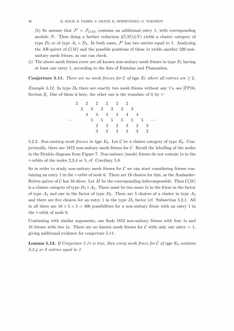
Example 5.12. In type D6 there are exactly two mesh friezes without any 1’s, see [FP16,
Section 3]. One of them is here, the other one is the translate of it by τ :
2 2 2 2 2 2
3 3 3 3 3 3
4 4 4 4 4 4
· · · 5 5 5 5 5 5 · · ·2 3 2 3 2 3
3 2 3 2 3 2
5.2.3. Non-unitary mesh friezes in type E8. Let C be a cluster category of type E8. Con-
jecturally, there are 1872 non-unitary mesh friezes for C. Recall the labelling of the nodes
in the Dynkin diagram from Figure 7. Non-unitary (mesh) friezes do not contain 1s in the
τ -orbits of the nodes 2,3,4 or 5, cf. Corollary 5.8.
So in order to study non-unitary mesh friezes for C we can start considering friezes con-
taining an entry 1 in the τ -orbit of node 6. There are 16 choices for this, as the Auslander-
Reiten quiver of C has 16 slices. Let M be the corresponding indecomposable. Then C(M)
is a cluster category of type D5×A2. There must be two more 1s in the frieze in the factor
of type A2 and one in the factor of type D5. There are 5 choices of a cluster in type A2
and there are five choices for an entry 1 in the type D5 factor (cf. Subsection 5.2.1. All
in all there are 16 × 5 × 5 = 400 possibilities for a non-unitary frieze with an entry 1 in
the τ -orbit of node 6.
Continuing with similar arguments, one finds 1852 non-unitary friezes with four 1s and
16 friezes with two 1s. There are no known mesh friezes for C with only one entry = 1,
giving additional evidence for conjecture 5.11:
Lemma 5.13. If Conjecture 5.11 is true, then every mesh frieze for C of type E8 contains
0,2,4 or 8 entries equal to 1.
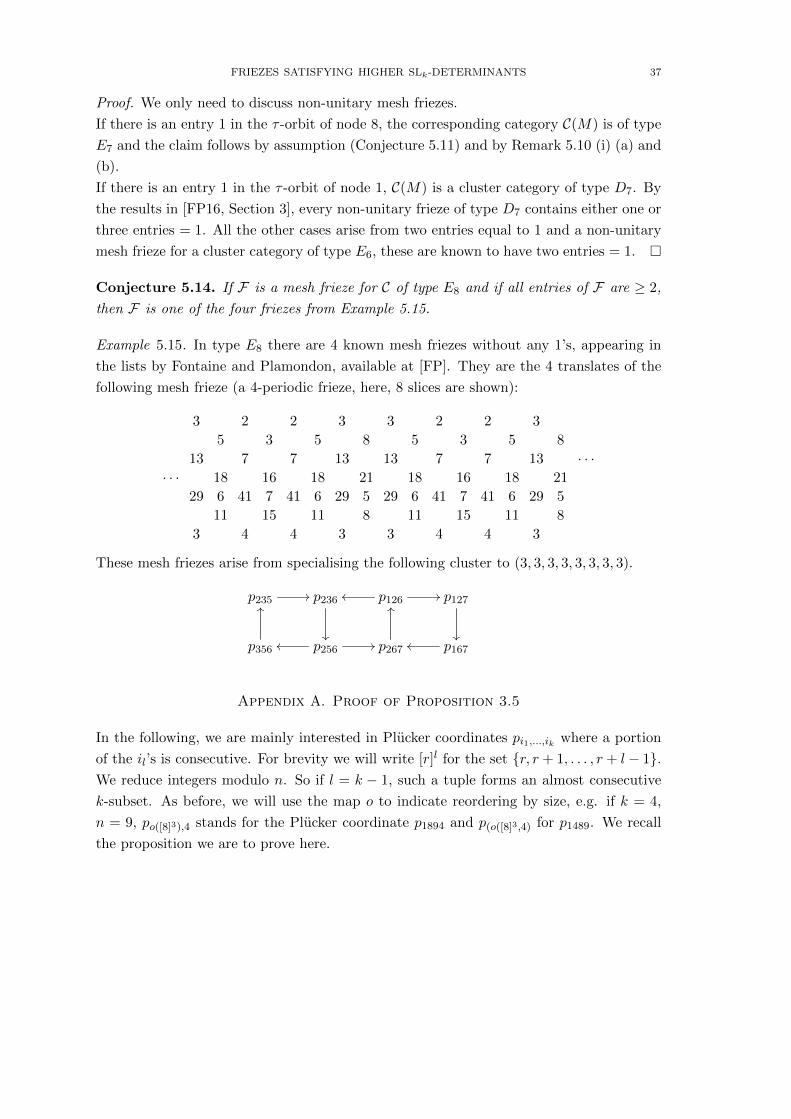
FRIEZES SATISFYING HIGHER SLk-DETERMINANTS 37
Proof. We only need to discuss non-unitary mesh friezes.
If there is an entry 1 in the τ -orbit of node 8, the corresponding category C(M) is of type
E7 and the claim follows by assumption (Conjecture 5.11) and by Remark 5.10 (i) (a) and
(b).
If there is an entry 1 in the τ -orbit of node 1, C(M) is a cluster category of type D7. By
the results in [FP16, Section 3], every non-unitary frieze of type D7 contains either one or
three entries = 1. All the other cases arise from two entries equal to 1 and a non-unitary
mesh frieze for a cluster category of type E6, these are known to have two entries = 1. �
Conjecture 5.14. If F is a mesh frieze for C of type E8 and if all entries of F are ≥ 2,
then F is one of the four friezes from Example 5.15.
Example 5.15. In type E8 there are 4 known mesh friezes without any 1’s, appearing in
the lists by Fontaine and Plamondon, available at [FP]. They are the 4 translates of the
following mesh frieze (a 4-periodic frieze, here, 8 slices are shown):
3 2 2 3 3 2 2 3
5 3 5 8 5 3 5 8
13 7 7 13 13 7 7 13 · · ·· · · 18 16 18 21 18 16 18 21
29 6 41 7 41 6 29 5 29 6 41 7 41 6 29 5
11 15 11 8 11 15 11 8
3 4 4 3 3 4 4 3
These mesh friezes arise from specialising the following cluster to (3, 3, 3, 3, 3, 3, 3, 3).
p235 // p236
��
p126 //oo p127
��p356
OO
p256 //oo p267
OO
p167oo
Appendix A. Proof of Proposition 3.5
In the following, we are mainly interested in Plucker coordinates pi1,...,ik where a portion
of the il’s is consecutive. For brevity we will write [r]l for the set {r, r + 1, . . . , r + l− 1}.We reduce integers modulo n. So if l = k − 1, such a tuple forms an almost consecutive
k-subset. As before, we will use the map o to indicate reordering by size, e.g. if k = 4,
n = 9, po([8]3),4 stands for the Plucker coordinate p1894 and p(o([8]3,4) for p1489. We recall
the proposition we are to prove here.
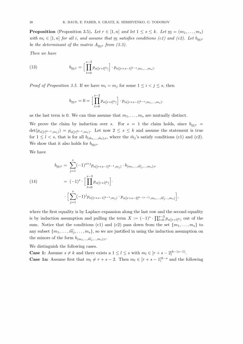
38 K. BAUR, E. FABER, S. GRATZ, K. SERHIYENKO, G. TODOROV
Proposition (Proposition 3.5). Let r ∈ [1, n] and let 1 ≤ s ≤ k. Let m = (m1, . . . ,ms)
with mi ∈ [1, n] for all i, and assume that m satisfies conditions (c1) and (c2). Let bm;r
be the determinant of the matrix Am;r from (3.3).
Then we have
bm;r =[ s−2∏l=0
po([r+l]k)
]· po([r+s−1]k−s,m1,...,ms).(13)
Proof of Proposition 3.5. If we have mi = mj for some 1 ≤ i < j ≤ s, then
bm;r = 0 =[ s−2∏l=0
po([r+l]k)
]· po([r+s−1]k−s,m1,...,ms).
as the last term is 0. We can thus assume that m1, . . . ,ms are mutually distinct.
We prove the claim by induction over s. For s = 1 the claim holds, since bm;r =
det(po([r]k−1,m1)) = po([r]k−1,m1). Let now 2 ≤ s ≤ k and assume the statement is true
for 1 ≤ l < s, that is for all b(m1,...,ml);s, where the mj ’s satisfy conditions (c1) and (c2).
We show that it also holds for bm;r.
We have
(14)
bm;r =s∑
j=1
(−1)s+jpo([r+s−1]k−1,mj) · b(m1,...,mj ,...,ms);r
= (−1)s ·[ s−3∏l=0
po([r+l]k)
]·
·[ s∑j=1
(−1)jpo([r+s−1]k−1,mj) · po([r+s−2]k−(s−1),m1,...,mj ...,ms)
],
where the first equality is by Laplace expansion along the last row and the second equality
is by induction assumption and pulling the term X := (−1)s ·∏s−3
l=0 po([r+l]k) out of the
sum. Notice that the conditions (c1) and (c2) pass down from the set {m1, . . . ,ms} to
any subset {m1, . . . , mj , . . . ,ms}, so we are justified in using the induction assumption on
the minors of the form b(m1,...,mj ,...,ms);r.
We distinguish the following cases.
Case 1: Assume s 6= k and there exists a 1 ≤ l ≤ s with ml ∈ [r + s− 2]k−(s−1).
Case 1a: Assume first that ml 6= r + s − 2. Then ml ∈ [r + s − 1]k−s and the following

FRIEZES SATISFYING HIGHER SLk-DETERMINANTS 39
expressions all vanish:
po([r+s−1]k−1,ml)= po([r+s−1]k−s,m1,...,ms) = 0
and p[r+s−2]k−(s−1),m1,...,mj ...,ms= 0 for all j 6= l.
Combining this with Equation (14) it follows that
bm;r = 0 =s−2∏l=0
po([r+l]k) · po([r+s−1]k−s,m1,...,ms).
This proves the claim in this case.
Case 1b: Assume now that ml = r+s−2 and l < s. If we had ml+1 ∈ (r+k−2,ml], then
we would have r+ k− 2 ∈ (ml,ml+1) ⊆ (m1,ms) contradicting condition (c2). Therefore,
we must have ml+1 ∈ (ml, r + k − 2] = [r + s − 1]k−s and we are in case 1a with ml+1
taking on the role of ml.
Case 1c: As a last subcase for case 1 assume that l = s and ms = r + s − 2. Then all
terms in (14) with factors po([r+s−2]k−(s−1),m1,...,mj ,...,ms)with j 6= s vanish and we obtain
bm;r = (−1)s ·[ s−3∏l=0
po([r+l]k)
]·
· (−1)spo([r+s−1]k−1,ms) · po([r+s−2]k−(s−1),m1,...,ms−1),
=[ s−2∏l=0
po([r+l]k)
]· po([r+s−1]k−s,m1,...,ms),
where the second equality follows directly from the equality ms = r + s− 2. This proves
the claim in this case.
Case 2: Assume now s = k and there exists a 1 ≤ l ≤ k such that ml = r + k − 2. This
cannot happen if l 6= k: By condition (c2) we have r+ k− 2 /∈ [m1,mk), but by condition
(c1), we have ml ∈ [m1,mk) for 1 ≤ l < k. Therefore, ml = r + k − 2 implies l = k, and
thus in Case 2 we have mk = r + k − 2. Then the same argument as in case 1c, replacing
s by k, proves the claim.
Case 3: We are now left with the case where ml /∈ [r+ s− 2]k−(s−1) for all 1 ≤ l ≤ s. We
are going to show that
s∑j=1
(−1)jpo([r+s−1]k−1,mj) · po([r+s−2]k−(s−1),m1,...mj ...,ms)=
(−1)s · po([r+s−2]k) · po([r+s−1]k−s,m1,...,ms),
(15)
which, when substituting into (14) yields the desired equality (13). We use the Plucker
relations on I = [r + s − 1]k−1 of cardinality |I| = k − 1 and J = [r + s − 2]k−(s−1) ∪

40 K. BAUR, E. FABER, S. GRATZ, K. SERHIYENKO, G. TODOROV
{m1,m2, . . . ,ms} of cardinality |J | = k + 1.
Case 3a: Assume that 1 = r + a ∈ [r + s− 1]k−1 ∩ [r + s− 2]k−(s−1). Then I is ordered
as follows:
1 = r + a < r + a+ 1 < . . . < r + s+ k − 3 < r + s− 1 < . . . < r + a− 1
and J is ordered as follows:
1 = r + a < r + a+ 1 < . . . < r + k − 2 < m1 < m2 < . . . < ms
< r + s− 2 < r + s− 1 < . . . < r + a− 1 = n.
Notice that we must have m1 < ml for all l 6= 1. Otherwise, if there exists a 1 < l ≤ s
with ml < m1, then if we have ml ∈ [1, r+k−2] ⊆ [r+s−2, r+k−2] this contradicts the
assumptions of case 3, and if we have ml ∈ (r+k−2, n], then it follows from ml < m1 that
r + k − 2 ∈ [m1,ml) ⊆ [m1,ms), which contradicts condition (c2). The Plucker relation
on I and J (cf. Equation (1)) thus reads as:
0 =k−a−2∑l=0
(−1)l · po([r+s−1]k−1),r+a+l · po(J\{r+a+l})
+s∑
l=1
(−1)k−a−2+l · po([r+s−1]k−1),ml· po(J\ml)
+
a−s+1∑l=0
(−1)k−a+s+l−1 · po([r+s−1]k−1),r+s−2+l · po(J\{r+s−2+l}).
Notice that po([r+s−1]k−1),r+j = 0 for all j ∈ [s − 1, k − 2] and thus the whole first sum
among those three vanishes, and all the summands, except for the first one (l = 0) in the
last sum vanish as well. The Plucker relation thus reduces to
0 =s∑
l=1
(−1)k−a−2+l · po([r+s−1]k−1),ml· po(J\ml)
+ (−1)k−a+s−1 · po([r+s−1]k−1),r+s−2 · po([r+s−1]k−s,m1,...,ms).
We need to get the remaining k-tuples in linear order. Observe that
po([r+s−1]k−1,ml)=pr+a,...,r+s+k−3,ml,r+s−1,...,r+a−1
= sgn(π)po([r+s−1]k−1),ml
and
po([r+s−2]k) =(r + a, . . . , r + s+ k − 3, r + s− 2, r + s− 1, . . . , r + a− 1)
= sgn(π)po([r+s−1]k−1),r+s−2
FRIEZES SATISFYING HIGHER SLk-DETERMINANTS 41
where π = (s+ k − a− 1, s+ k − a, . . . , k − 1, k) ∈ Sk. Substituting this into the Plucker
relation on I and J (and multiplying by sign(π) · (−1)k−a) yields
0 =s∑
l=1
(−1)l · po([r+s−1]k−1,ml)· po(J\ml)
− (−1)s · po([r+s−2]k) · po([r+s−1]k−s,m1,...,ms),
which, observing that po(J\ml) = po([r+s−2]k−(s−1),m1,...,ml,...,ms)and pulling the second term
to the left hand side yields the desired Equation (15).
Case 3b: For the final case, assume that 1 /∈ [r + s− 1]k−1 ∩ [r + s− 2]k−(s−1). We first
observe what the linear order on J looks like. Notice that we have r+ s− 2 < r+ s− 1 <
. . . < r+k−2. Since mj /∈ [r+s−2, r+k−2], the set J is ordered in one of the following
three ways (16), (17), (18):
mb < mb+1 < . . . < ms < r + s− 2 < . . . < r + k − 2 < m1 < m2 < . . . < mb−1,(16)
for some b ∈ {2, . . . , s},
m1 < m2 < . . . < ms < r + s− 2 < . . . < r + k − 2, or(17)
r + s− 2 < . . . < r + k − 2 < m1 < . . . < ms.(18)
If it is ordered as in (17), we set b = 1, and if it is ordered as in (18), we set b = s + 1.
Then the Plucker relation on I and J reads as follows:
0 =
s∑l=b
(−1)l−bpo(〈[r+s−1]k−1),ml· po(J\ml)
+k−s∑l=0
(−1)s−b+1+l · po([r+s−1]k−1),r+s−2+l · po(J\{r+s−2+l})
+b−1∑l=1
(−1)k−b+1+l · po([r+s−1]k−1),ml· po(J\ml).
Notice again that po([r+s−1]k−1),r+j = 0 for all j ∈ [s − 1, k − 2], and therefore the cor-
responding terms in the Plucker relation vanish. Again, we need to get the remaining
k-tuples in linear order. Observe that
po([r+s−1]k−1),ml=
{po([r+s−1]k−1,ml)
if 1 ≤ l ≤ b− 1
sgn(σ)po([r+s−1]k−1,ml)if b ≤ l ≤ s
and that po([r+s−1]k−1),r+s−2 = sgn(σ)po([r+s−2]k), where σ = (1, 2, . . . , k) ∈ Sk with
sgn(σ) = (−1)k−1. Therefore, if J is ordered as in (17) or (18) the Plucker relation
42 K. BAUR, E. FABER, S. GRATZ, K. SERHIYENKO, G. TODOROV
on I and J can be rewritten as
0 =
s∑l=b
(−1)l−b · (−1)k−1po([r+s−1]k−1,ml)· po(J\ml)
+ (−1)s−b+1 · (−1)k−1po([r+s−2]k) · po(J\{r+s−2})
+b−1∑l=1
(−1)k−b+1+l · po([r+s−1]k−1,ml)· po(J\ml),
Juggling the signs in a straight forward way, and pulling together the first and last sum
we obtain
0 =(−1)s · (−1)k−b · po([r+s−2]k) · po(J\{r+s−2})
+ (−1)k−b+1s∑
l=1
(−1)l · po([r+s−1]k−1,ml)· po(J\ml).
Pulling the second term on the left hand side and multiplying by (−1)k−b yields as desired
Equality (15), observing that po(J\ml) = po([r+s−2]k−(s−1),m1,...,ml,...,ms). This concludes the
proof. �
Appendix B. Counting friezes in type E6
Michael Cuntz#, Pierre-Guy Plamondon†
Friezes (also called “friezes of type A” and “SL2-friezes”) were introduced by H. Coxeter in
[Cox71] and later studied by H. Coxeter and J. Conway in [CC73a, CC73b]. It was observed
by P. Caldero that the theory of cluster algebras of S. Fomin and A. Zelevinsky [FZ02a]
allows for a far-reaching generalization of the original notion of frieze; this generalization
was first studied in [ARS10]. Recall that in [ARS10], a frieze (of Dynkin type) is a mesh
frieze on an associated Auslander-Reiten quiver, cf. Remark 4.11. Since then, many
generalizations and variations on the notion of friezes have been introduced, as can be
seen in the survey paper [MG15].
It is known that, for a given non-Dynkin type, there are infinitely many friezes of that
type. However, it follows from [CC73a, CC73b] that friezes of Dynkin type A come in
a finite number (given by Catalan numbers), and it was proved in [FP16] that friezes of
Dynkin type B,D and G also come in a finite (explicit) number (the result for type D4
was also proved in [MGOT12]). It was conjectured in [Pro05, MGOT12, FP16] that the
number of friezes in type E6 is 868; in [FP16] the precise number of friezes in any Dynkin
type is also conjectured.
FRIEZES SATISFYING HIGHER SLk-DETERMINANTS 43
In this Appendix, we settle the case of type E6, and obtain the result for type F4 as a
corollary.
Theorem B.1. The number of friezes of type E6 is exactly 868.
Since Dynkin type F4 is a folding of type E6, it follows from the work of [FP16] that we
then have:
Corollary B.1. The number of friezes of type F4 is exactly 112.
Our proof relies on a reduction to 2-friezes (whose definition we recall below); our strategy
is to show that the entries in a 2-frieze of height 3 are bounded.
We have attempted to apply the methods used in this Appendix to types E7 and E8,
without success.
B.1. 2-friezes
We shall not be using the definition of a frieze from [ARS10], but rather a slightly different
notion, that of a 2-frieze as defined in [MGOT12].
Definition B.2. A 2-frieze of height h is an array of positive integers (ai,j), where
• i ∈ Z and j ∈ {0, 1, . . . , h+ 1};• for all i ∈ Z, we have that ai,0 = ai,h+1 = 1;
• for all i ∈ Z and all j ∈ {1, . . . , h}, we have that ai,j = ai−1,jai+1,j − ai,j−1ai,j+1.
The reason we are interested in 2-friezes is the following result, which is a consequence of
[MGOT12, Proposition 5.4] and of the fact that the quiver depicted in [MGOT12, (2.3)]
is mutation-equivalent to a quiver of type E6.
Theorem B.2 ([MGOT12]). Entries in a 2-frieze of height 3 are entries in a frieze of
type E6 which determine the frieze. This defines an injection from the set of friezes of
type E6 to the set of 2-friezes of height 3.
Our strategy to prove Theorem B.1 is thus to prove that the number of 2-friezes of height 3
is finite. We will do this by showing that there is a bound on the possible values appearing
in a 2-frieze of height 3.
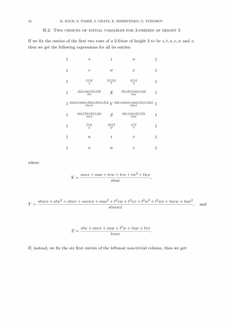
44 K. BAUR, E. FABER, S. GRATZ, K. SERHIYENKO, G. TODOROV
B.2. Two choices of initial variables for 2-friezes of height 3
If we fix the entries of the first two rows of a 2-frieze of height 3 to be s, t, u, v, w and x,
then we get the following expressions for all its entries:
1 s t u 1
1 v w x 1
1 v+ws
vx+wt
w+xu 1
1 svx+sw+tv+twstv X tw+tx+uvx+uw
tux 1
1 suvx+suw+tuw+tvw+tvxtuvw Y stw+suvx+suw+tvx+twx
stwx 1
1 sux+tw+tx+uwuwx Z suv+sw+tv+tw
svw 1
1 t+ux
su+tw
s+tv 1
1 u t s 1
1 x w v 1
where
X =suvx+ suw + tvw + tvx+ tw2 + twx
stuw,
Y =stuvx+ stw2 + stwx+ suvwx+ suw2 + t2vw + t2vx+ t2w2 + t2wx+ tuvw + tuw2
stuvwx, and
Z =stw + suvx+ suw + t2w + tuw + tvx
tvwx.
If, instead, we fix the six first entries of the leftmost non-trivial column, then we get:
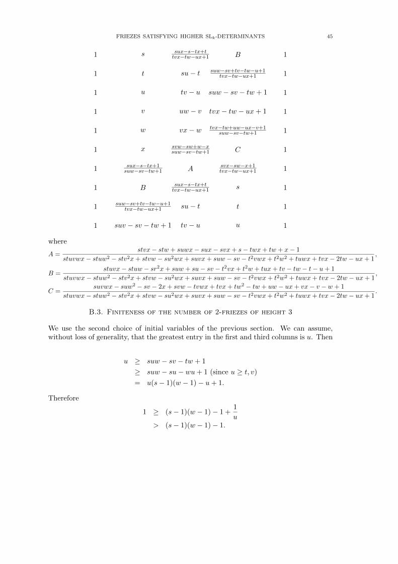
FRIEZES SATISFYING HIGHER SLk-DETERMINANTS 45
1 s sux−s−tx+ttvx−tw−ux+1 B 1
1 t su− t suw−sv+tv−tw−u+1tvx−tw−ux+1 1
1 u tv − u suw − sv − tw + 1 1
1 v uw − v tvx− tw − ux+ 1 1
1 w vx− w tvx−tw+uw−ux−v+1suw−sv−tw+1 1
1 x svw−sw+w−xsuw−sv−tw+1 C 1
1 sux−s−tx+1suw−sv−tw+1 A
svx−sw−x+1tvx−tw−ux+1 1
1 Bsux−s−tx+ttvx−tw−ux+1 s 1
1 suw−sv+tv−tw−u+1tvx−tw−ux+1 su− t t 1
1 suv − sv − tw + 1 tv − u u 1
where
A =stvx− stw + suwx− sux− svx+ s− twx+ tw + x− 1
stuvwx− stuw2 − stv2x+ stvw − su2wx+ suvx+ suw − sv − t2vwx+ t2w2 + tuwx+ tvx− 2tw − ux+ 1,
B =stuvx− stuw − sr2x+ suw + su− sv − t2vx+ t2w + tux+ tv − tw − t− u+ 1
stuvwx− stuw2 − stv2x+ stvw − su2wx+ suvx+ suw − sv − t2vwx+ t2w2 + tuwx+ tvx− 2tw − ux+ 1,
C =suvwx− suw2 − sv − 2x+ svw − tvwx+ tvx+ tw2 − tw + uw − ux+ vx− v − w + 1
stuvwx− stuw2 − stv2x+ stvw − su2wx+ suvx+ suw − sv − t2vwx+ t2w2 + tuwx+ tvx− 2tw − ux+ 1.
B.3. Finiteness of the number of 2-friezes of height 3
We use the second choice of initial variables of the previous section. We can assume,without loss of generality, that the greatest entry in the first and third columns is u. Then
u ≥ suw − sv − tw + 1
≥ suw − su− wu+ 1 (since u ≥ t, v)
= u(s− 1)(w − 1)− u+ 1.
Therefore
1 ≥ (s− 1)(w − 1)− 1 +1
u> (s− 1)(w − 1)− 1.
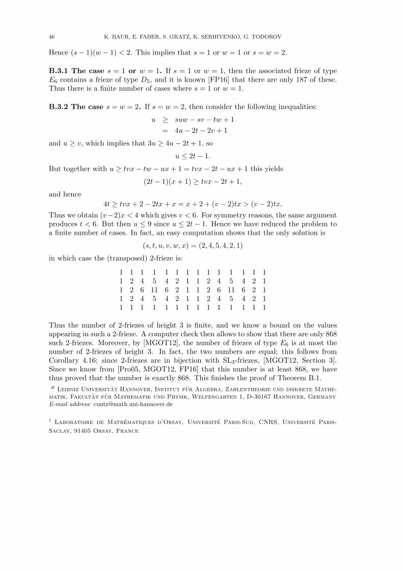
46 K. BAUR, E. FABER, S. GRATZ, K. SERHIYENKO, G. TODOROV
Hence (s− 1)(w − 1) < 2. This implies that s = 1 or w = 1 or s = w = 2.
B.3.1 The case s = 1 or w = 1. If s = 1 or w = 1, then the associated frieze of typeE6 contains a frieze of type D5, and it is known [FP16] that there are only 187 of these.Thus there is a finite number of cases where s = 1 or w = 1.
B.3.2 The case s = w = 2. If s = w = 2, then consider the following inequalities:
u ≥ suw − sv − tw + 1
= 4u− 2t− 2v + 1
and u ≥ v, which implies that 3u ≥ 4u− 2t+ 1, so
u ≤ 2t− 1.
But together with u ≥ tvx− tw − ux+ 1 = tvx− 2t− ux+ 1 this yields
(2t− 1)(x+ 1) ≥ tvx− 2t+ 1,
and hence
4t ≥ tvx+ 2− 2tx+ x = x+ 2 + (v − 2)tx > (v − 2)tx.
Thus we obtain (v−2)x < 4 which gives v < 6. For symmetry reasons, the same argumentproduces t < 6. But then u ≤ 9 since u ≤ 2t− 1. Hence we have reduced the problem toa finite number of cases. In fact, an easy computation shows that the only solution is
(s, t, u, v, w, x) = (2, 4, 5, 4, 2, 1)
in which case the (transposed) 2-frieze is:
1 1 1 1 1 1 1 1 1 1 1 1 1 11 2 4 5 4 2 1 1 2 4 5 4 2 11 2 6 11 6 2 1 1 2 6 11 6 2 11 2 4 5 4 2 1 1 2 4 5 4 2 11 1 1 1 1 1 1 1 1 1 1 1 1 1
Thus the number of 2-friezes of height 3 is finite, and we know a bound on the valuesappearing in such a 2-frieze. A computer check then allows to show that there are only 868such 2-friezes. Moreover, by [MGOT12], the number of friezes of type E6 is at most thenumber of 2-friezes of height 3. In fact, the two numbers are equal; this follows fromCorollary 4.16; since 2-friezes are in bijection with SL3-friezes, [MGOT12, Section 3].Since we know from [Pro05, MGOT12, FP16] that this number is at least 868, we havethus proved that the number is exactly 868. This finishes the proof of Theorem B.1.# Leibniz Universitat Hannover, Institut fur Algebra, Zahlentheorie und diskrete Mathe-
matik, Fakultat fur Mathematik und Physik, Welfengarten 1, D-30167 Hannover, GermanyE-mail address: [email protected]
† Laboratoire de Mathematiques d’Orsay, Universite Paris-Sud, CNRS, Universite Paris-
Saclay, 91405 Orsay, France
FRIEZES SATISFYING HIGHER SLk-DETERMINANTS 47
E-mail address: [email protected]
References
[Ami09] Claire Amiot. Cluster categories for algebras of global dimension 2 and quivers with potential.Ann. Inst. Fourier (Grenoble), 59(6):2525–2590, 2009.
[ARS10] Ibrahim Assem, Christophe Reutenauer, and David Smith. Friezes. Adv. Math., 225(6):3134–3165, 2010.
[BBGE19] Karin Baur, Dusko Bogdanic, and Ana Garcia Elsener. Cluster categories from Grassmanni-ans and root combinatorics. Nagoya Mathematical Journal, pages 1–33, 2019.
[BM09] Karin Baur and Robert J. Marsh. Frieze patterns for punctured discs. J. Algebraic Combin.,30(3):349–379, 2009.
[BMR+06] Aslak Bakke Buan, Robert Marsh, Markus Reineke, Idun Reiten, and Gordana Todorov.Tilting theory and cluster combinatorics. Adv. Math., 204(2):572–618, 2006.
[BPT16] Karin Baur, Mark J. Parsons, and Manuela Tschabold. Infinite friezes. European J. Combin.,54:220–237, 2016.
[BR10] Francois Bergeron and Christophe Reutenauer. SLk-tilings of the plane. Illinois J. Math.,54(1):263–300, 2010.
[Buc86] Ragnar-Olaf Buchweitz. Maximal Cohen–Macaulay modules and Tate cohomology overGorenstein rings. unpublished manuscript, 1986.
[CC73a] John H. Conway and Harold S. M. Coxeter. Triangulated polygons and frieze patterns. Math.Gaz., 57(400):87–94, 1973.
[CC73b] John H. Conway and Harold S.M. Coxeter. Triangulated polygons and frieze patterns. Math.Gaz., 57(401):175–183, 1973.
[CC06] Philippe Caldero and Frederic Chapoton. Cluster algebras as Hall algebras of quiver repre-sentations. Comment. Math. Helv., 81(3):595–616, 2006.
[CL17] P. Cao and F. Lin. Positivity of denominator vectors of cluster algebras. 2017. https://
arxiv.org/pdf/1712.06975.pdf.[Cox71] Harold S. M. Coxeter. Frieze patterns. Acta Arith., 18:297–310, 1971.[CR72] Craig M. Cordes and D. P. Roselle. Generalized frieze patterns. Duke Math. J., 39:637–648,
1972.[Cun17] Michael Cuntz. On wild frieze patterns. Exp. Math., 26(3):342–348, 2017.[DL16] Laurent Demonet and Xueyu Luo. Ice quivers with potential associated with triangulations
and Cohen-Macaulay modules over orders. Trans. Amer. Math. Soc., 368(6):4257–4293, 2016.[FP] Bruce Fontaine and Pierre-Guy Plamondon. Lists of friezes of finite type. https://www.math.
u-psud.fr/~plamondon/friezes/.[FP16] Bruce Fontaine and Pierre-Guy Plamondon. Counting friezes in type Dn. J. Algebraic Com-
bin., 44(2):433–445, 2016.[FZ02a] Sergey Fomin and Andrei Zelevinsky. Cluster algebras. I. Foundations. J. Amer. Math. Soc.,
15(2):497–529, 2002.[FZ02b] Sergey Fomin and Andrei Zelevinsky. The Laurent phenomenon. Adv. in Appl. Math.,
28(2):119–144, 2002.[FZ03] Sergey Fomin and Andrei Zelevinsky. Y -systems and generalized associahedra. Ann. of Math.
(2), 158(3):977–1018, 2003.[GHKK18] Mark Gross, Paul Hacking, Sean Keel, and Maxim Kontsevich. Canonical bases for cluster
algebras. J. Amer. Math. Soc., 31(2):497–608, 2018.[GLS13] Christof Geiss, Bernard Leclerc, and Jan Schroer. Factorial cluster algebras. Doc. Math.,
18:249–274, 2013.
48 K. BAUR, E. FABER, S. GRATZ, K. SERHIYENKO, G. TODOROV
[Hap88] Dieter Happel. Triangulated categories in the representation theory of finite-dimensional alge-bras, volume 119 of London Mathematical Society Lecture Note Series. Cambridge UniversityPress, Cambridge, 1988.
[IY08] Osamu Iyama and Yuji Yoshino. Mutation in triangulated categories and rigid Cohen-Macaulay modules. Invent. Math., 172(1):117–168, 2008.
[JKS16] Bernt Tore Jensen, Alastair D. King, and Xiuping Su. A categorification of Grassmanniancluster algebras. Proc. Lond. Math. Soc. (3), 113(2):185–212, 2016.
[LS15] Kyungyong Lee and Ralf Schiffler. Positivity for cluster algebras. Ann. of Math. (2),182(1):73–125, 2015.
[Mar13] Robert J. Marsh. Lecture notes on cluster algebras. Zurich Lectures in Advanced Mathematics.European Mathematical Society (EMS), Zurich, 2013.
[MG12] Sophie Morier-Genoud. Arithmetics of 2-friezes. J. Algebraic Combin., 36(4):515–539, 2012.[MG15] Sophie Morier-Genoud. Coxeter’s frieze patterns at the crossroads of algebra, geometry and
combinatorics. Bull. Lond. Math. Soc., 47(6):895–938, 2015.[MGOST14] Sophie Morier-Genoud, Valentin Ovsienko, Richard Evan Schwartz, and Serge Tabachnikov.
Linear difference equations, frieze patterns, and the combinatorial Gale transform. ForumMath. Sigma, 2:e22, 45, 2014.
[MGOT12] Sophie Morier-Genoud, Valentin Ovsienko, and Serge Tabachnikov. 2-frieze patterns and thecluster structure of the space of polygons. Ann. Inst. Fourier (Grenoble), 62(3):937–987, 2012.
[MSW11] Gregg Musiker, Ralf Schiffler, and Lauren Williams. Positivity for cluster algebras from sur-faces. Adv. Math., 227(6):2241–2308, 2011.
[Pro05] James Propp. The combinatorics of frieze patterns and Markoff numbers. 2005. https://
arxiv.org/abs/math/0511633.[Sco06] Jeanne Scott. Grassmannians and cluster algebras. Proc. London Math. Soc. (3), 92(2):345–
380, 2006.
School of Mathematics, University of Leeds, Leeds, LS2 9JT, UK. On leave from the Uni-versity of Graz, Austria
E-mail address: [email protected]
School of Mathematics, University of Leeds, Leeds, LS2 9EJ, UK
E-mail address: [email protected]
School of Mathematics and Statistics, University of Glasgow, University Place, Glasgow,G12 8SQ, UK
E-mail address: [email protected]
Department of Mathematics, University of California at Berkeley, Berkeley, CA 94720,USA
E-mail address: [email protected]
Department of Mathematics, Northeastern University, Boston, MA 02115, USA
E-mail address: [email protected]