INTERNATIONAL SOLVAY INSTITUTES FOR PHYSICS AND CHEMISTRY

Proceedings of the Symposium Henri Poincare (Brussels, 8-9 October 2004)

From dynamical systems theory tononequilibrium thermodynamics

Pierre Gaspard

Center for Nonlinear Phenomena and Complex Systems,Universite Libre de Bruxelles,Code Postal 231, Campus Plaine,B-1050 Brussels, BelgiumEmail: gaspard@ulb.ac.be

Abstract. An overview is given of recent advances on diffusion andnonequilibrium thermodynamics in the perspective given by the pioneer-ing work of Henri Poincare on dynamical systems theory. The hydrody-namic modes of diffusion are explicitly constructed from the underlyingdeterministic dynamics in the multibaker, the hard-disk and Yukawa-potential Lorentz gases, as well as in a geodesic flow on a noncompactmanifold of constant negative curvature built out of the Poincare disk.These modes are represented by singular distributions with fractal cu-mulative functions.

1 Introduction

The purpose of the present paper is to give an overview of the contributions ofHenri Poincare to dynamical systems theory and its modern developments inthe theory of chaos and our current understanding of the dynamical bases ofnonequilibrium thermodynamics.

Poincare is the founding father of modern dynamical systems theory by hismonumental work on celestial mechanics. The fundamental concepts he hasintroduced still plays a central role in this field and beyond. By inventing theconcept of homoclinic orbit and by describing for the first time a homoclinictangle, Poincare discovered what is today referred to as dynamical chaos. Thisis a particular state of motion in which most of the trajectories are random al-though they are solutions of a deterministic dynamical systems defined in termsof regular differential equations or maps. Chaotic motion has been discoveredin Hamiltonian, conservative, and dissipative dynamical systems with a few ormany degrees of freedom. Many disciplines are concerned with dynamical chaosfrom mathematics to natural sciences such as physics, chemistry, meteorologyand geophysics, or biology where many examples of chaotic systems have beendiscovered and studied.

In the present paper, the focus will be on dynamical systems of interestfor the transport properties and, in particular, the property of diffusion, whichis of interest for nonequilibrium statistical mechanics. Diffusion is a processof transport of particles across a spatially extended system. If the motion ischaotic, the particle may perform a random walk due to its successive colli-sions with scatterers. The process of diffusion is described in nonequilibriumthermodynamics as an irreversible process responsible for entropy production.For this reason, deterministic dynamical systems with diffusion constitute in-teresting models to investigate mechanisms leading to irreversible behavior asdescribed by nonequilibrium thermodynamics. This program has been success-fully carried out for simple models, leading to a very precise understanding ofentropy production in the case of diffusion [1–6]. It has been discovered thatit is possible to construct so-called hydrodynamic modes of diffusion from thechaotic dynamics. These modes are defined as generalized eigenstates of the Li-ouvillian or Frobenius-Perron operators ruling the time evolution of statisticalensembles of trajectories. The associated eigenvalues, also called the Pollicott-Ruelle resonances, give the damping rates of the modes and they control therelaxation toward the state of thermodynamics equilibrium. These generalizedeigenstates are not given by regular functions contrary what might be expected:they are given by singular mathematical distributions with fractal properties.The singular character of these eigenstates has been shown to be responsiblefor the entropy irreversibly produced by diffusion during the relaxation towardequilibrium, as expected from nonequilibrium thermodynamics. The irreversiblecharacter is understood by the fact that the eigenstates break the time-reversalsymmetry. Indeed, the eigenstates are smooth along the unstable manifolds ofthe chaotic dynamics but singular along the stable manifolds. Therefore, theyare distinct from their image under time reversal.

In the present paper, these eigenstates representing the hydodynamic modesof diffusion are presented for different systems: the multibaker map which is asimplified model of diffusion, the hard-disk and Yukawa-potential Lorentz gases,and finally for a geodesic flow on a negative curvature space. This last example

2

is constructed in the Poincare disk of nonEuclidean geometry. All these systemshave in common to be spatially periodic so that their Liouvillian dynamics canbe analyzed by spatial Fourier transforms, leading to the explicit constructionof the Liouvillian eigenstates and associated eigenvalues. These results provideone of the most advanced understanding of the dynamical bases of kinetic theoryand nonequilibrium thermodynamics.

The plan of the paper is the following. In Sec. 2, an overview is given ofPoincare’s contributions to dynamical systems theory. Remarkably, Poincarehas also contributions to gas kinetic theory which are reviewed in Sec. 3. InSec. 4, it is shown that dynamical chaos is very common in systems of statisticalmechanics. The aim of Sec. 5 is to explain how time-reversal symmetry can bebroken in a theory based on an equation having the invariance. The constructionof the hydrodynamic modes of diffusion is carried out in Sec. 6 where they areshown to have fractal properties. This construction is applied to the multibakermap and the Lorentz gases in Sec. 7. In Sec. 8, diffusion is presented fora geodesic flow on a negative curvature space. Finally, the implications forentropy production and nonequilibrium thermodynamics are discussed in Sec.9 and conclusions are drawn in Sec. 10.

2 Poincare and dynamical systems theory

Henri Poincare is considered as the founding father of dynamical systems theorybecause he has discovered many basic results of immediate use for the qualitativeand quantitative analyses of dynamical systems. The advent of modern com-puters has allowed us to explicitly and numerically construct the phase-spaceobjects discovered by Poincare. Poincare’s advances into dynamical systemstheory are due to his efforts to understand the stability of the Solar Systemand, in particular, the problem of three bodies in gravitational interaction. Hismemoir for the King Oscar Prize in 1888 has led to the publications in 1892,1893 and 1899 of his famous three-volume work entitled Les methodes nouvellesde la mecanique celeste (The novel methods of celestial mechanics). Today, thiswork is still the source of inspiration for active research in celestial mechanicsand dynamical systems theory. Some of the most recent spatial missions are us-ing complicated orbits meandering through phase-space chaotic zones in orderto minimize fuel.

Some of the main contributions of Poincare to dynamical systems theory arethe following results and concepts:

• the Poincare-Bendixson theorem which proves the absence of chaos intwo-dimensional flows;

• the Poincare surface of section which is a basic tool for the study of phase-space geometry;

• the stable Ws(γ) and unstable Wu(γ) invariant manifolds of an orbit γ;

• the homoclinic orbit which is defined by Poincare as the intersectionWs(γ) ∩Wu(γ) between the stable and unstable manifolds of an orbit γ,as well as the heteroclinic orbit defined as the intersection Ws(γ)∩Wu(γ′)of the stable manifold of an orbit γ with the unstable manifold of anotherorbit γ′;

3

• the homoclinic tangle which is the phase-space figure formed by the in-tersecting stable and unstable manifolds of a set of orbits and which is atthe origin of chaotic behavior in three-dimensional flows. Poincare gavea description of the homoclinic tangle in his book but only modern workhas provided concrete visualization of homoclinic tangles.

These concepts were developed later, notably, by Birkhoff and Shil’nikovwho proved the existence of periodic and nonperiodic orbits in the vicinityof a homoclinic orbit. This led to the notion of symbolic dynamics in whichsequences of symbols can be associated with the trajectories of the system.In this way, it became possible to list and enumerate the trajectories. If thesequences are freely built on the basis of an alphabet with several symbols,the periodic orbits proliferate exponentially as their period increases. The rateof exponential proliferation is the so-called topological entropy per unit time,which provides a quantitative topological characterization of chaotic behavior.These properties concern both conservative and dissipative dynamical systems.

3 Poincare and gas kinetic theory

Poincare published few papers on gas kinetic theory. They reflect the extraordi-nary dynamism of Poincare to follow the scientific developments of his time but,contrary to other fields where Poincare could anticipate, his papers on gas kinetictheory appear as comments on previous contributions by others. In the years1892-1894, Poincare wrote a few critical comments about Maxwell’s approach,which attests that a definitive mathematical formulation of the experimentalfacts was still lacking in those years [7].

Later, Poincare published in 1906 a paper entitled Reflexions sur la theoriecinetique des gaz (Thoughts on gas kinetic theory) [8], which cites GibbsO con-tribution of 1902 [9]. This paper contains a version of what is today calledLiouville’s equation. For the time evolution of the phase-space probability den-sity P(xi, t), Poincare uses the continuity equation

∂P∂t

+∑

i

∂(PXi)∂xi

= 0 (1)

corresponding to a dynamical system defined by the ordinary differential equa-tions

dxi

dt= Xi (2)

For a system obeying Liouville’s theorem∑i

∂Xi

∂xi= 0 (3)

he also gives the form∂P∂t

+∑

i

Xi∂P∂xi

= 0 (4)

which Gibbs wrote in 1902 as

∂P∂t

= −∑

k

(∂P∂pk

pk +∂P∂qk

qk

)(5)

4

with xi = (pk, qk) [9]. A consensus on the basic equation of statisticalmechanics is thus clearly emerging during these years. Liouville’s equation canalso be written as

∂P∂t

= H,P ≡ LP (6)

in terms of the Poisson bracket ·, · of the Hamiltonian H with the probabilitydensity P, which defines the Liouvillian operator L.

Besides, Poincare’s 1906 paper mainly contains a discussion of the behaviorof the coarse-grained and fine-grained entropies in an ideal gas in the absenceor presence of an external perturbation. For this model, Poincare discusses inparticular about the constancy of the fine-grained entropy in the absence ofexternal perturbation and the increase in time of the coarse-grained entropy.The conclusions of the paper expresses Poincare’s appreciation that, with suchresults, the last difficulties of gas kinetic theory finally disappear [8].

Poincare also published a treatise on thermodynamics which contains atthe end a discussion of his viewpoint about the deduction of the principles ofthermodynamics from those of mechanics [10].

It should be added that Poincare published his famous recurrence theoremin 1890 in the context of the three-body problem and it was Zermelo who, in1896, used this theorem as an objection to Boltzmann’s H-theorem, a debateto which Poincare did not directly participate.

4 Chaotic behavior in molecular dynamics

The merging of dynamical systems theory and chaos theory with modern sta-tistical mechanics occurred much later. During the twenties and the thir-ties, ergodic theory underwent important developments with contributions fromBirkhoff, Hedlund, Hopf, Koopman, von Neumann, Seidel, and others. On theone hand, these developments contributed to define rigorously the notions ofergodicity and of mixing and, on the other hand, they showed that these sta-tistical properties manifest themselves in hyperbolic dynamical systems such asgeodesic motions on closed surfaces of constant negative curvature.

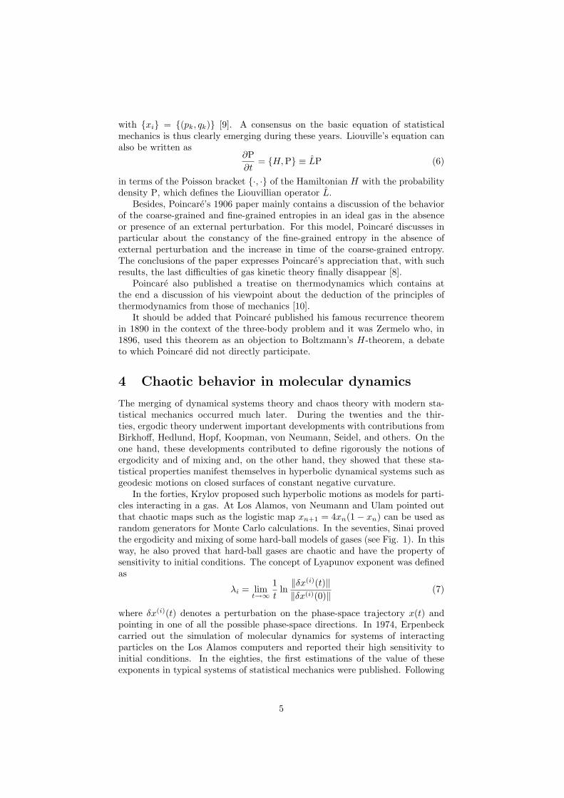
In the forties, Krylov proposed such hyperbolic motions as models for parti-cles interacting in a gas. At Los Alamos, von Neumann and Ulam pointed outthat chaotic maps such as the logistic map xn+1 = 4xn(1− xn) can be used asrandom generators for Monte Carlo calculations. In the seventies, Sinai provedthe ergodicity and mixing of some hard-ball models of gases (see Fig. 1). In thisway, he also proved that hard-ball gases are chaotic and have the property ofsensitivity to initial conditions. The concept of Lyapunov exponent was definedas

λi = limt→∞

1t

ln‖δx(i)(t)‖‖δx(i)(0)‖

(7)

where δx(i)(t) denotes a perturbation on the phase-space trajectory x(t) andpointing in one of all the possible phase-space directions. In 1974, Erpenbeckcarried out the simulation of molecular dynamics for systems of interactingparticles on the Los Alamos computers and reported their high sensitivity toinitial conditions. In the eighties, the first estimations of the value of theseexponents in typical systems of statistical mechanics were published. Following

5

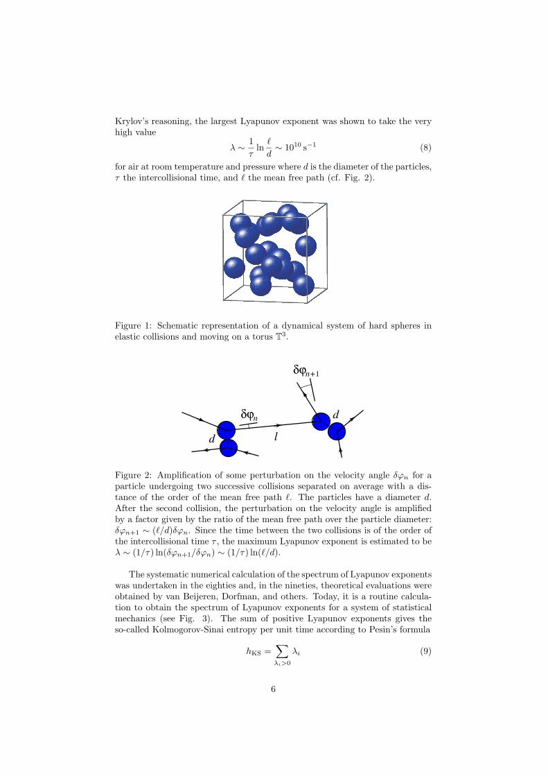
Krylov’s reasoning, the largest Lyapunov exponent was shown to take the veryhigh value

λ ∼ 1τ

ln`

d∼ 1010 s−1 (8)

for air at room temperature and pressure where d is the diameter of the particles,τ the intercollisional time, and ` the mean free path (cf. Fig. 2).

Figure 1: Schematic representation of a dynamical system of hard spheres inelastic collisions and moving on a torus T3.

d

d

l

δϕ

δϕ

n

n+1

Figure 2: Amplification of some perturbation on the velocity angle δϕn for aparticle undergoing two successive collisions separated on average with a dis-tance of the order of the mean free path `. The particles have a diameter d.After the second collision, the perturbation on the velocity angle is amplifiedby a factor given by the ratio of the mean free path over the particle diameter:δϕn+1 ∼ (`/d)δϕn. Since the time between the two collisions is of the order ofthe intercollisional time τ , the maximum Lyapunov exponent is estimated to beλ ∼ (1/τ) ln(δϕn+1/δϕn) ∼ (1/τ) ln(`/d).

The systematic numerical calculation of the spectrum of Lyapunov exponentswas undertaken in the eighties and, in the nineties, theoretical evaluations wereobtained by van Beijeren, Dorfman, and others. Today, it is a routine calcula-tion to obtain the spectrum of Lyapunov exponents for a system of statisticalmechanics (see Fig. 3). The sum of positive Lyapunov exponents gives theso-called Kolmogorov-Sinai entropy per unit time according to Pesin’s formula

hKS =∑λi>0

λi (9)

6

The Kolmogorov-Sinai entropy per unit time characterizes the dynamical ran-domness displayed by the trajectories of the total system of particles. It is theanalogue of the standard entropy per unit volume obtained by replacing spaceby time. In this regard, the Kolmogorov-Sinai entropy per unit time is a measureof time disorder in the dynamics of the system. The Kolmogorov-Sinai entropyis defined for the ergodic invariant probability measure of the thermodynamicequilibrium. It gives a lower bound on the topological entropy per unit time

hKS ≤ htop (10)

which is the rate of proliferation of unstable periodic orbits in the system. Eachof these periodic orbits has a stable manifold and an unstable manifold extendingin the phase space and intersecting with each other. The positive topologicalentropy per unit time inferred from Eqs. (9) and (10) implies the existence ofan important Poincare homoclinic tangle in the high-dimensional phase spaceof the systems of interacting particles.

0

0.02

0.04

0.06

0.08

0.1

0 20 40 60 80

+ positive exponents− negative exponents

No.

Ly

apu

no

v e

xp

on

ents

Figure 3: Spectrum of Lyapunov exponents of a dynamical system of 33 hardspheres of unit diameter and mass at unit temperature and density 0.001. TheLyapunov exponents obey the pairing rule that the Lyapunov exponents come inpairs λi,−λi. Eight Lyapunov exponents vanish because the system has fourconserved quantities, namely, energy and the three components of momentumand because of the pairing rule. The total number of Lyapunov exponents isequal to 6× 33 = 198.

5 Spontaneous breaking of time-reversal sym-metry and Pollicott-Ruelle resonances

Hamilton’s equations of motion are symmetric under time reversal Θ(pk, qk) =(−pk, qk). However, it is known that the solution of an equation may have a

7

lower symmetry than the equation itself. Accordingly, some invariant subsets ofphase space do not need to be time-reversal symmetric. For instance, Poincare’sinvariant stable and unstable manifolds of an orbit γ or of a set of orbits arenot symmetric under time reversal:

ΘWs = Wu 6= Ws (11)

This suggests that irreversible behavior may result from weighting differently thestable Ws and unstable Wu manifolds with a measure. This idea is at the basisof the concept of Pollicott-Ruelle resonance which has been rigorously definedfor Axiom-A systems [11, 12]. An Axiom-A system Φt satisfies the propertiesthat: (1) The nonwandering set Ω(Φt) is hyperbolic; (2) The periodic orbits ofΦt are dense in Ω(Φt). These systems are known to be strongly chaotic andmixing so that the mean values of the observables typically decay in time. ThePollicott-Ruelle resonances provide the decay rates of the time evolution. Theseresonances are the classical analogues of the quantum scattering resonances sincethey are the poles of the resolvent of the Liouvillian operator [13]

1s− L

(12)

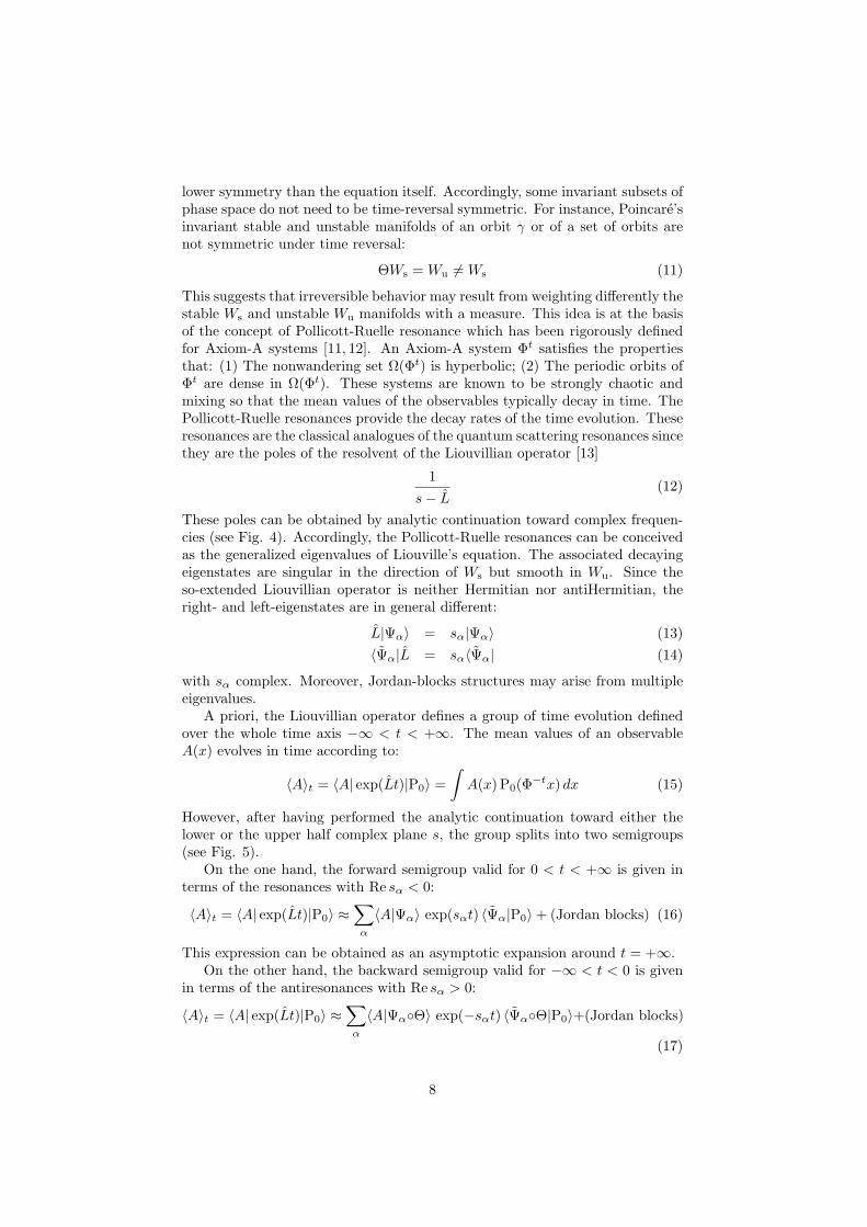
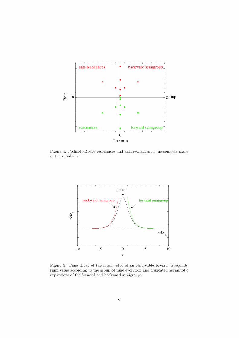
These poles can be obtained by analytic continuation toward complex frequen-cies (see Fig. 4). Accordingly, the Pollicott-Ruelle resonances can be conceivedas the generalized eigenvalues of Liouville’s equation. The associated decayingeigenstates are singular in the direction of Ws but smooth in Wu. Since theso-extended Liouvillian operator is neither Hermitian nor antiHermitian, theright- and left-eigenstates are in general different:

L|Ψα〉 = sα|Ψα〉 (13)〈Ψα|L = sα〈Ψα| (14)

with sα complex. Moreover, Jordan-blocks structures may arise from multipleeigenvalues.

A priori, the Liouvillian operator defines a group of time evolution definedover the whole time axis −∞ < t < +∞. The mean values of an observableA(x) evolves in time according to:

〈A〉t = 〈A| exp(Lt)|P0〉 =∫

A(x) P0(Φ−tx) dx (15)

However, after having performed the analytic continuation toward either thelower or the upper half complex plane s, the group splits into two semigroups(see Fig. 5).

On the one hand, the forward semigroup valid for 0 < t < +∞ is given interms of the resonances with Re sα < 0:

〈A〉t = 〈A| exp(Lt)|P0〉 ≈∑α

〈A|Ψα〉 exp(sαt) 〈Ψα|P0〉+ (Jordan blocks) (16)

This expression can be obtained as an asymptotic expansion around t = +∞.On the other hand, the backward semigroup valid for −∞ < t < 0 is given

in terms of the antiresonances with Re sα > 0:

〈A〉t = 〈A| exp(Lt)|P0〉 ≈∑α

〈A|ΨαΘ〉 exp(−sαt) 〈ΨαΘ|P0〉+(Jordan blocks)

(17)

8

0

0

Re s

Im s = ω

resonances

anti-resonances backward semigroup

forward semigroup

group

Figure 4: Pollicott-Ruelle resonances and antiresonances in the complex planeof the variable s.

-10 -5 0 5 10

<A

>t

t

<A>eq

forward semigroupbackward semigroup

group

Figure 5: Time decay of the mean value of an observable toward its equilib-rium value according to the group of time evolution and truncated asymptoticexpansions of the forward and backward semigroups.

9

It is obtained as an asymptotic expansion around t = −∞. The time-reversalsymmetry implies that a resonance sα corresponds to each antiresonance −sα.However, the associated eigenstates Ψα and Ψα Θ differ because the formeris smooth along the unstable manifolds though the latter is smooth along thestable ones. Hence, these eigenstates break the time-reversal symmetry. We arein the presence of a phenomenon of broken symmetry very similar to other suchphenomena known in condensed-matter physics.

6 Diffusion in spatially extended systems

We now consider dynamical systems which are spatially extended and which cansustain a transport process of diffusion. We moreover assume that the systemis invariant under a discrete abelian subgroup of spatial translations a. Theinvariance of the Liouvillian time evolution under this subgroup means thatthe Perron-Frobenius operator P t = exp(Lt) commutes with the translationoperators T a: [

P t, T a]

= 0 (18)

Consequently, these operators admit common eigenstates:P tΨk = exp(skt)Ψk

T aΨk = exp(ik · a)Ψk(19)

where k is called the wavenumber or Bloch parameter. The Pollicott-Ruelleresonances are now functions of the wavenumber. For strongly chaotic systemswith two degrees of freedom, the resonances can be obtained as the roots of thedynamical zeta function:

Z(s;k) =∏p

∞∏m=0

(1− exp(−sTp − ik · ap)

|Λp|Λmp

)m+1

(20)

which is given by a product over all the unstable periodic orbits p of instabilityeigenvalue Λp and prime period Tp. The lattice vector ap gives the spatialdistance travelled by the particle along the prime period of the periodic orbit p.

The leading Pollicott-Ruelle resonance which vanishes with the wavenumberdefines the dispersion relation of diffusion:

sk = −Dk2 + O(k4) (21)

The diffusion coefficient is given by the Green-Kubo formula:

D =∫ ∞

0

〈vx(0)vx(t)〉 dt (22)

where vx is the velocity of the diffusing particle. The associated eigenstate isthe hydrodynamic mode of diffusion Ψk.

6.1 Fractality of the hydrodynamic modes of diffusion

In strongly chaotic systems, the diffusive eigenstate Ψk is a Schwartz-type dis-tribution which is smooth in the unstable direction Wu but singular in Ws. This

10

distribution cannot be depicted except by its cumulative function

Fk(θ) =∫ θ

0

Ψk(xθ′) dθ′ (23)

defined by integrating over a curve xθ in the phase space (with 0 ≤ θ < 2π).We notice that the eigenstate Ψk of the forward semigroup can be obtained byapplying the time evolution operator over an arbitrary long time from an initialfunction which is spatially periodic of wavenumber k whereupon the cumulativefunction (23) is equivalently defined by

Fk(θ) = limt→∞

∫ θ

0dθ′ exp [ik · (rt − r0)θ′ ]∫ 2π

0dθ′ exp [ik · (rt − r0)θ′ ]

(24)

This function is normalized to take the unit value for θ = 2π. For vanishingwavenumber, the cumulative function is equal to Fk(θ) = θ/(2π), which is thecumulative function of the microcanonical uniform distribution in phase space.For nonvanishing wavenumbers, the cumulative function becomes complex.

Examples of such cumulative functions of the hydrodynamic modes of dif-fusion are depicted in the following for several dynamical systems of chaoticdiffusion. These cumulative functions typically form fractal curves in the com-plex plane (Re Fk, Im Fk). It has been proved that the Hausdorff dimension DH

of these fractal curves can be calculated by the formula:

P(DH) = DH Re sk (25)

in terms of the Ruelle topological pressure:

P(β) ≡ limt→∞

1t

ln 〈|Λt|1−β〉 (26)

where Λt is the factor by which the phase-space volume are stretched along theunstable direction [5]. The positive Lyapunov exponent is given by

λ = −P ′(1) = limt→∞

1t〈ln |Λt|〉 (27)

The system is closed so that there is no escape of particles and P (1) = 0. TheHausdorff dimension can be expanded in powers of the wavenumber as

DH(k) = 1 +Dλ

k2 +O(k4) (28)

so that the diffusion coefficient can be obtained from the Hausdorff dimensionand the Lyapunov exponent by the formula

D = λ limk→0

DH(k)− 1k2

(29)

This formula has been verified for different dynamical systems sustaining deter-ministic diffusion [5].

11

7 Examples of diffusive modes

In the present section, we explicitly construct the hydrodynamic modes of dif-fusion for several spatially periodic dynamical systems. All the systems are ofHamiltonian character so that they are time-reversal symmetric and obey Li-ouville’s theorem. These systems have two degrees of freedom and are chaoticso that they have the Lyapunov spectrum (λ, 0, 0,−λ) where λ is the uniquepositive Lyapunov exponent.

7.1 Multibaker model of diffusion

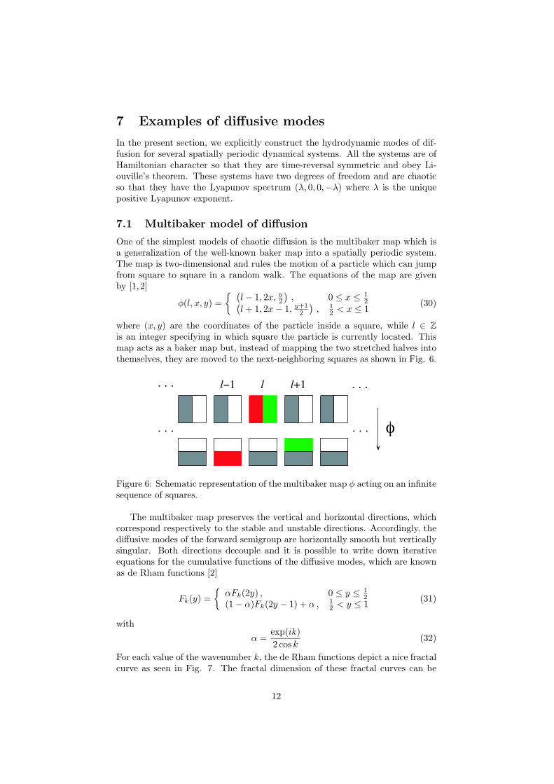
One of the simplest models of chaotic diffusion is the multibaker map which isa generalization of the well-known baker map into a spatially periodic system.The map is two-dimensional and rules the motion of a particle which can jumpfrom square to square in a random walk. The equations of the map are givenby [1,2]

φ(l, x, y) = (

l − 1, 2x, y2

), 0 ≤ x ≤ 1

2(l + 1, 2x− 1, y+1

2

), 1

2 < x ≤ 1(30)

where (x, y) are the coordinates of the particle inside a square, while l ∈ Zis an integer specifying in which square the particle is currently located. Thismap acts as a baker map but, instead of mapping the two stretched halves intothemselves, they are moved to the next-neighboring squares as shown in Fig. 6.

φ. . . . . .

ll−1 l+1. . . . . .

Figure 6: Schematic representation of the multibaker map φ acting on an infinitesequence of squares.

The multibaker map preserves the vertical and horizontal directions, whichcorrespond respectively to the stable and unstable directions. Accordingly, thediffusive modes of the forward semigroup are horizontally smooth but verticallysingular. Both directions decouple and it is possible to write down iterativeequations for the cumulative functions of the diffusive modes, which are knownas de Rham functions [2]

Fk(y) =

αFk(2y) , 0 ≤ y ≤ 12

(1− α)Fk(2y − 1) + α , 12 < y ≤ 1 (31)

with

α =exp(ik)2 cos k

(32)

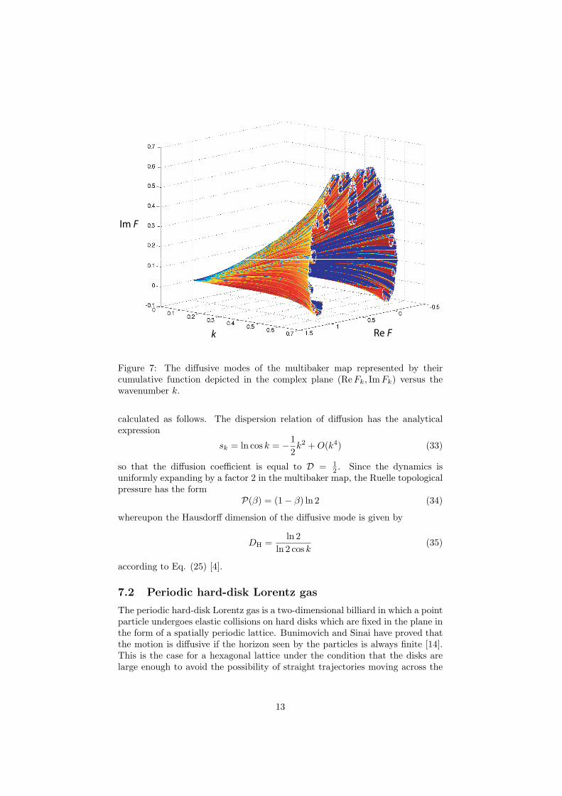
For each value of the wavenumber k, the de Rham functions depict a nice fractalcurve as seen in Fig. 7. The fractal dimension of these fractal curves can be

12

Re F

Im F

k

Figure 7: The diffusive modes of the multibaker map represented by theircumulative function depicted in the complex plane (Re Fk, Im Fk) versus thewavenumber k.

calculated as follows. The dispersion relation of diffusion has the analyticalexpression

sk = ln cos k = −12k2 + O(k4) (33)

so that the diffusion coefficient is equal to D = 12 . Since the dynamics is

uniformly expanding by a factor 2 in the multibaker map, the Ruelle topologicalpressure has the form

P(β) = (1− β) ln 2 (34)

whereupon the Hausdorff dimension of the diffusive mode is given by

DH =ln 2

ln 2 cos k(35)

according to Eq. (25) [4].

7.2 Periodic hard-disk Lorentz gas

The periodic hard-disk Lorentz gas is a two-dimensional billiard in which a pointparticle undergoes elastic collisions on hard disks which are fixed in the plane inthe form of a spatially periodic lattice. Bunimovich and Sinai have proved thatthe motion is diffusive if the horizon seen by the particles is always finite [14].This is the case for a hexagonal lattice under the condition that the disks arelarge enough to avoid the possibility of straight trajectories moving across the

13

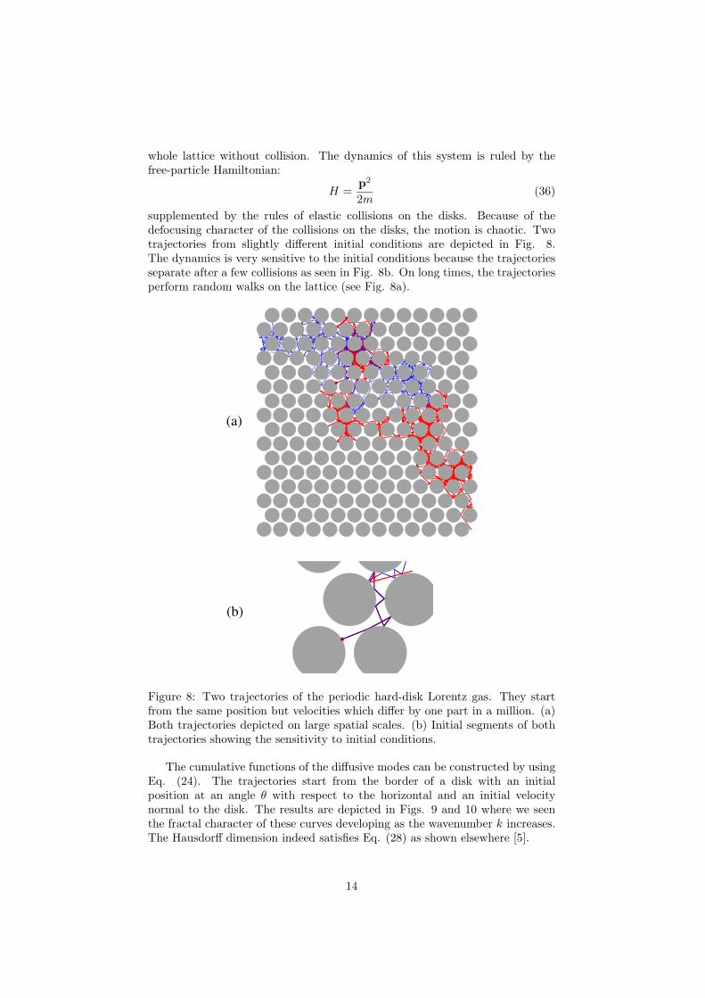
whole lattice without collision. The dynamics of this system is ruled by thefree-particle Hamiltonian:

H =p2

2m(36)

supplemented by the rules of elastic collisions on the disks. Because of thedefocusing character of the collisions on the disks, the motion is chaotic. Twotrajectories from slightly different initial conditions are depicted in Fig. 8.The dynamics is very sensitive to the initial conditions because the trajectoriesseparate after a few collisions as seen in Fig. 8b. On long times, the trajectoriesperform random walks on the lattice (see Fig. 8a).

(a)

(b)

Figure 8: Two trajectories of the periodic hard-disk Lorentz gas. They startfrom the same position but velocities which differ by one part in a million. (a)Both trajectories depicted on large spatial scales. (b) Initial segments of bothtrajectories showing the sensitivity to initial conditions.

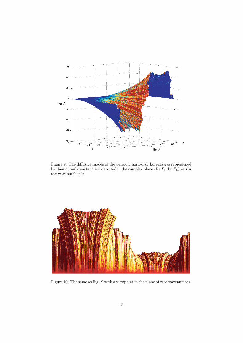
The cumulative functions of the diffusive modes can be constructed by usingEq. (24). The trajectories start from the border of a disk with an initialposition at an angle θ with respect to the horizontal and an initial velocitynormal to the disk. The results are depicted in Figs. 9 and 10 where we seenthe fractal character of these curves developing as the wavenumber k increases.The Hausdorff dimension indeed satisfies Eq. (28) as shown elsewhere [5].

14

Re F

Im F

k

Figure 9: The diffusive modes of the periodic hard-disk Lorentz gas representedby their cumulative function depicted in the complex plane (Re Fk, Im Fk) versusthe wavenumber k.

Figure 10: The same as Fig. 9 with a viewpoint in the plane of zero wavenumber.

15

7.3 Periodic Yukawa-potential Lorentz gas

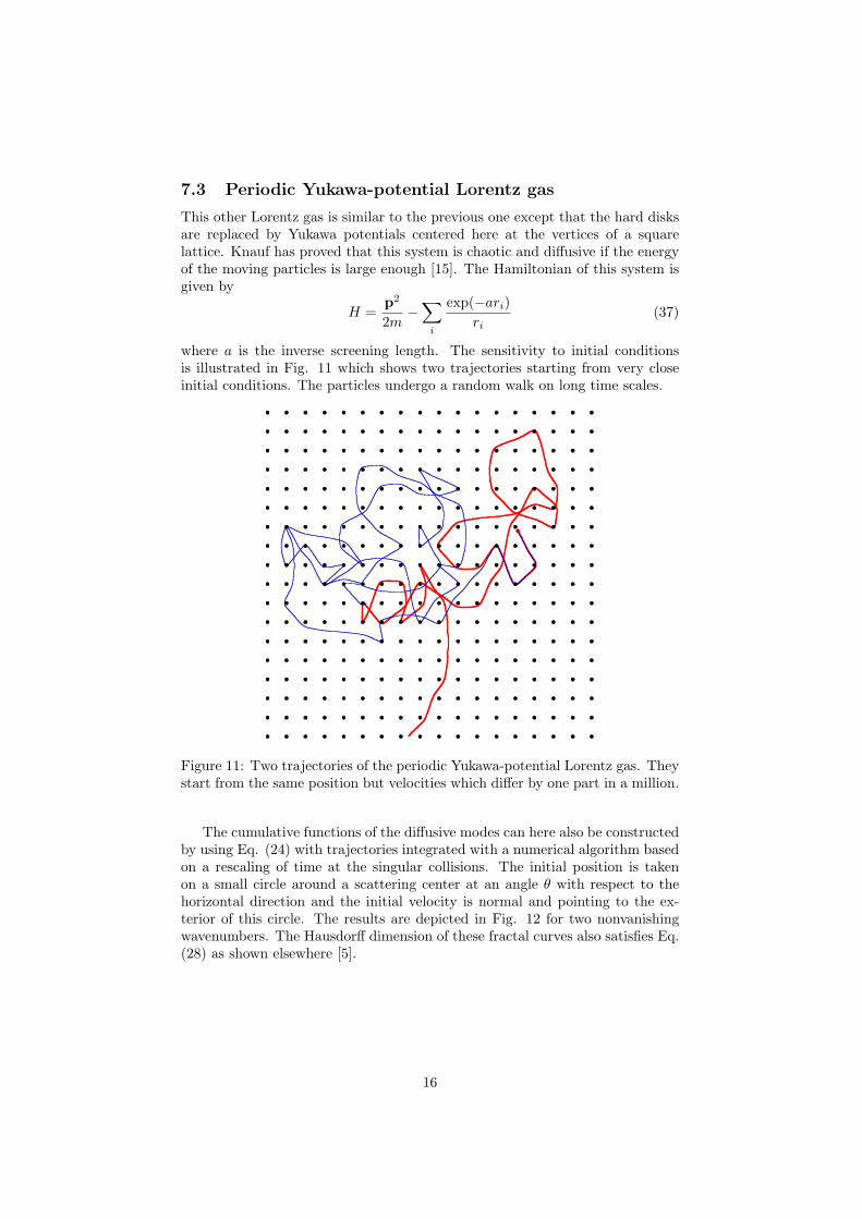
This other Lorentz gas is similar to the previous one except that the hard disksare replaced by Yukawa potentials centered here at the vertices of a squarelattice. Knauf has proved that this system is chaotic and diffusive if the energyof the moving particles is large enough [15]. The Hamiltonian of this system isgiven by

H =p2

2m−

∑i

exp(−ari)ri

(37)

where a is the inverse screening length. The sensitivity to initial conditionsis illustrated in Fig. 11 which shows two trajectories starting from very closeinitial conditions. The particles undergo a random walk on long time scales.

Figure 11: Two trajectories of the periodic Yukawa-potential Lorentz gas. Theystart from the same position but velocities which differ by one part in a million.

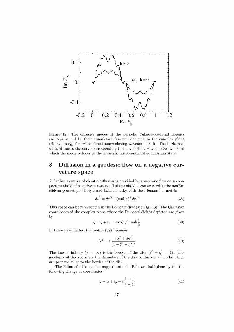
The cumulative functions of the diffusive modes can here also be constructedby using Eq. (24) with trajectories integrated with a numerical algorithm basedon a rescaling of time at the singular collisions. The initial position is takenon a small circle around a scattering center at an angle θ with respect to thehorizontal direction and the initial velocity is normal and pointing to the ex-terior of this circle. The results are depicted in Fig. 12 for two nonvanishingwavenumbers. The Hausdorff dimension of these fractal curves also satisfies Eq.(28) as shown elsewhere [5].

16

-0.1

0

0.1

-0.2 0 0.2 0.4 0.6 0.8 1 1.2

Im F

k

Re F k

k ≠ 0

eq. k = 0

Figure 12: The diffusive modes of the periodic Yukawa-potential Lorentzgas represented by their cumulative function depicted in the complex plane(Re Fk, Im Fk) for two different nonvanishing wavenumbers k. The horizontalstraight line is the curve corresponding to the vanishing wavenumber k = 0 atwhich the mode reduces to the invariant microcanonical equilibrium state.

8 Diffusion in a geodesic flow on a negative cur-vature space

A further example of chaotic diffusion is provided by a geodesic flow on a com-pact manifold of negative curvature. This manifold is constructed in the nonEu-clidean geometry of Bolyai and Lobatchevsky with the Riemannian metric:

ds2 = dτ2 + (sinh τ)2 dϕ2 (38)

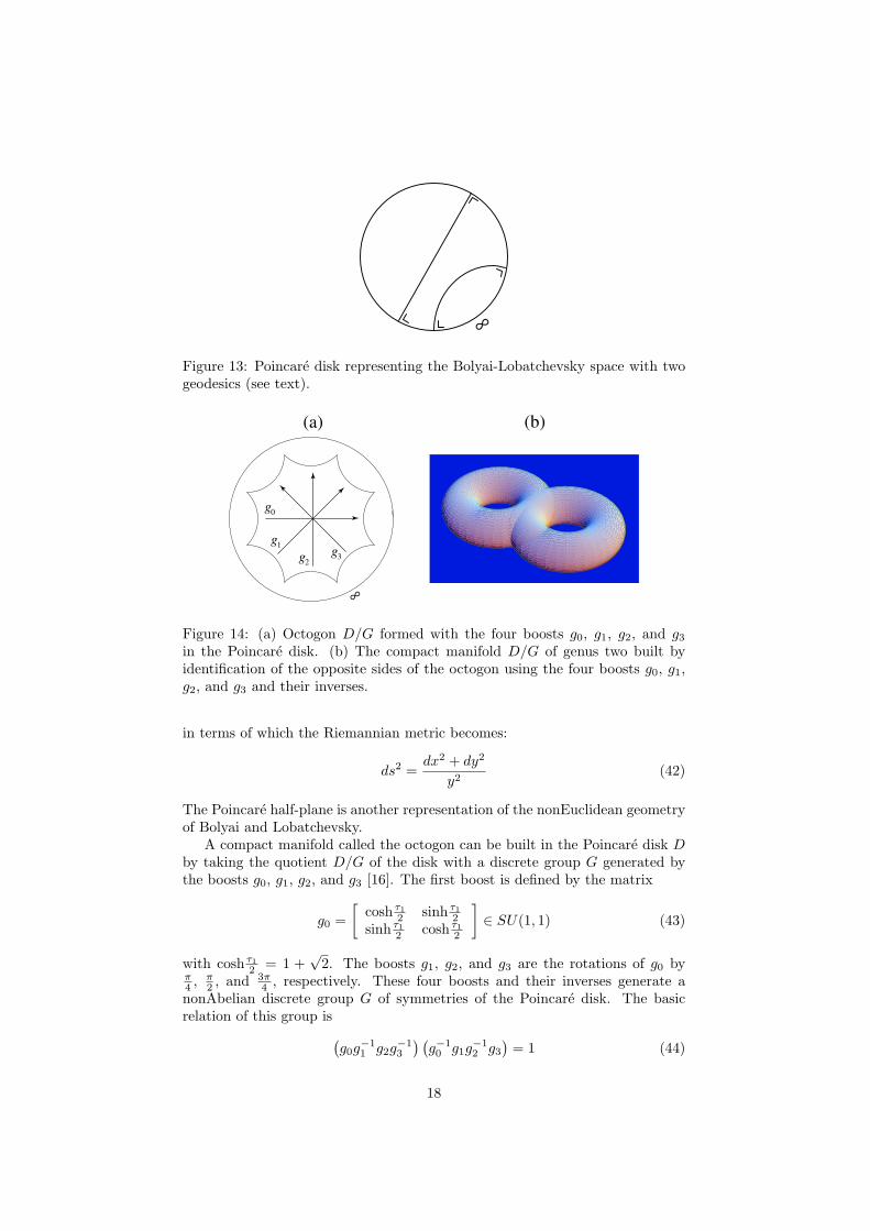
This space can be represented in the Poincare disk (see Fig. 13). The Cartesiancoordinates of the complex plane where the Poincare disk is depicted are givenby

ζ = ξ + iη = exp(iϕ) tanhτ

2(39)

In these coordinates, the metric (38) becomes

ds2 = 4dξ2 + dη2

(1− ξ2 − η2)2(40)

The line at infinity (τ = ∞) is the border of the disk (ξ2 + η2 = 1). Thegeodesics of this space are the diameters of the disk or the arcs of circles whichare perpendicular to the border of the disk.

The Poincare disk can be mapped onto the Poincare half-plane by the thefollowing change of coordinates

z = x + iy = i1− ζ

1 + ζ(41)

17

∞

Figure 13: Poincare disk representing the Bolyai-Lobatchevsky space with twogeodesics (see text).

g0

g1

g2

g3

∞

(a) (b)

Figure 14: (a) Octogon D/G formed with the four boosts g0, g1, g2, and g3

in the Poincare disk. (b) The compact manifold D/G of genus two built byidentification of the opposite sides of the octogon using the four boosts g0, g1,g2, and g3 and their inverses.

in terms of which the Riemannian metric becomes:

ds2 =dx2 + dy2

y2(42)

The Poincare half-plane is another representation of the nonEuclidean geometryof Bolyai and Lobatchevsky.

A compact manifold called the octogon can be built in the Poincare disk Dby taking the quotient D/G of the disk with a discrete group G generated bythe boosts g0, g1, g2, and g3 [16]. The first boost is defined by the matrix

g0 =[

cosh τ12 sinh τ1

2sinh τ1

2 cosh τ12

]∈ SU(1, 1) (43)

with cosh τ12 = 1 +

√2. The boosts g1, g2, and g3 are the rotations of g0 by

π4 , π

2 , and 3π4 , respectively. These four boosts and their inverses generate a

nonAbelian discrete group G of symmetries of the Poincare disk. The basicrelation of this group is(

g0g−11 g2g

−13

) (g−10 g1g

−12 g3

)= 1 (44)

18

Each boost can be used to map onto each other two opposite circles perpendicu-lar to the border of the disk as shown in Fig. 14a. The eight circles intersect toform a curvilinear octogon. The opposite sides of this octogon can be identifiedwith the four boosts and their inverses in order to define a compact manifold ofgenus two depicted in Fig. 14b.

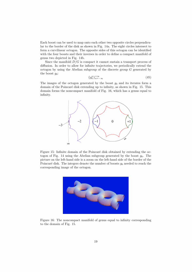
Since the manifold D/G is compact it cannot sustain a transport process ofdiffusion. In order to allow for infinite trajectories, we periodically extend theoctogon by using the Abelian subgroup of the discrete group G generated bythe boost g0:

gn0 +∞n=−∞ (45)

The images of the octogon generated by the boost g0 and its iterates form adomain of the Poincare disk extending up to infinity, as shown in Fig. 15. Thisdomain forms the noncompact manifold of Fig. 16, which has a genus equal toinfinity.

∞

∞

0 +1−1−2

−3

Figure 15: Infinite domain of the Poincare disk obtained by extending the oc-togon of Fig. 14 using the Abelian subgroup generated by the boost g0. Thepicture on the left-hand side is a zoom on the left-hand side of the border of thePoincare disk. The integers denote the number of boosts g0 needed to reach thecorresponding image of the octogon.

Figure 16: The noncompact manifold of genus equal to infinity correspondingto the domain of Fig. 15.

19

-150

-100

-50

0

50

0 1 104

2 104

3 104

nu

mb

er

of

bo

osts

g0

discrete time

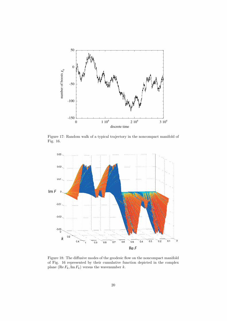
Figure 17: Random walk of a typical trajectory in the noncompact manifold ofFig. 16.

Re F

Im F

k

Figure 18: The diffusive modes of the geodesic flow on the noncompact manifoldof Fig. 16 represented by their cumulative function depicted in the complexplane (Re Fk, Im Fk) versus the wavenumber k.

20

Diffusive motion is now possible on this noncompact surface. Figure 17depicts the position of a typical trajectory measured by the number of boostsg0. A central limit theorem rules the number of boosts g0 after a long time andthis motion has a positive and finite diffusion coefficient.

The hydrodynamic modes of diffusion of this system are constructed by usingEq. (24) with trajectories starting from the center of the Poincare disk withvelocities making an angle θ with respect to the horizontal axis. The results aredepicted in Fig. 18, which shown the same fractality of the cumulative functionsas for the multibaker map and the Lorentz gases.

In conclusion, the theory of the diffusive modes is very general and appliesto a broad variety of different dynamical systems.

9 Entropy production and irreversibility

The study of the hydrodynamic modes of diffusion as eigenstates of the Li-ouvillian operator has shown that these modes are typically given in terms ofsingular distributions without density function. Since the works by Gelfand,Schwartz, and others in the fifties it is known that such distributions acquire amathematical meaning if they are evaluated for some test functions belongingto certain classes of functions. The test function used to evaluate a distributionis arbitrary although the distribution is not. Examples of test functions arethe indicator functions of the cells of some partition of phase space. In thisregard, the singular character of the diffusive modes justifies the introductionof a coarse-graining procedure. This reasoning goes along the need to carry outa coarse graining in order to understand that entropy increases with time, asunderstood by Gibbs [9] and Poincare [8] at the beginning of the XXth century.

If a phase-space region Ml is partitioned into cells A, the probability thatthe system is found in the cell A at time t is given by

µt(A) =∫

A

P(x, t)dx (46)

in terms of the probability density P(x, t) which evolves in time according toLiouville’s equation. If the underlying dynamics has Gibbs’ mixing property,these probabilities converge to their equilibrium value at long times:

limt→±∞

µt(A) = µeq(A) (47)

The knowledge of the Pollicott-Ruelle resonances ±sα of the forward or back-ward semigroups allows us to specify the approach to the equilibrium state interms of the following time asymptotics for t → ±∞:

µt(A) = µeq(A) +∑α

C±α exp(±sαt) + · · · (48)

where the coefficients C±α are calculated using the eigenstates associated withthe resonances (see Fig. 5).

The coarse-grained entropy is defined in terms of the probabilities as

St(Ml|A) = −kB

∑A

µt(A) lnµt(A) (49)

21

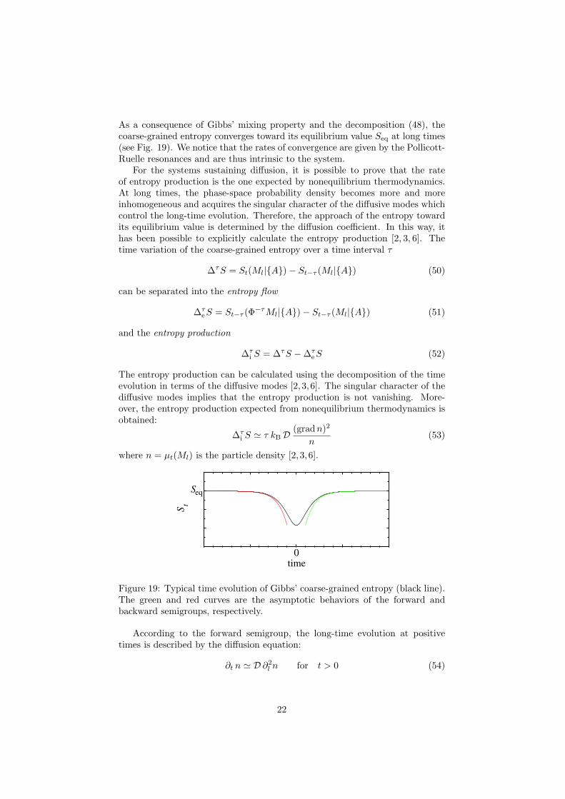
As a consequence of Gibbs’ mixing property and the decomposition (48), thecoarse-grained entropy converges toward its equilibrium value Seq at long times(see Fig. 19). We notice that the rates of convergence are given by the Pollicott-Ruelle resonances and are thus intrinsic to the system.

For the systems sustaining diffusion, it is possible to prove that the rateof entropy production is the one expected by nonequilibrium thermodynamics.At long times, the phase-space probability density becomes more and moreinhomogeneous and acquires the singular character of the diffusive modes whichcontrol the long-time evolution. Therefore, the approach of the entropy towardits equilibrium value is determined by the diffusion coefficient. In this way, ithas been possible to explicitly calculate the entropy production [2, 3, 6]. Thetime variation of the coarse-grained entropy over a time interval τ

∆τS = St(Ml|A)− St−τ (Ml|A) (50)

can be separated into the entropy flow

∆τeS = St−τ (Φ−τMl|A)− St−τ (Ml|A) (51)

and the entropy production

∆τi S = ∆τS −∆τ

eS (52)

The entropy production can be calculated using the decomposition of the timeevolution in terms of the diffusive modes [2, 3, 6]. The singular character of thediffusive modes implies that the entropy production is not vanishing. More-over, the entropy production expected from nonequilibrium thermodynamics isobtained:

∆τi S ' τ kBD

(gradn)2

n(53)

where n = µt(Ml) is the particle density [2, 3, 6].

0

St

time

Seq

Figure 19: Typical time evolution of Gibbs’ coarse-grained entropy (black line).The green and red curves are the asymptotic behaviors of the forward andbackward semigroups, respectively.

According to the forward semigroup, the long-time evolution at positivetimes is described by the diffusion equation:

∂t n ' D ∂2l n for t > 0 (54)

22

In contrast, it is an antidiffusion equation which describes the long-time evolu-tion at negative times according to the backward semigroup:

∂t n ' −D ∂2l n for t < 0 (55)

Consequently, the entropy increases toward its equilibrium value for both t →±∞ (see Fig. 19). The fact is that the forward and backward semigroupsinvolve Liouvillian eigenstates which are physically distinct. Indeed, the eigen-states of the forward semigroup are smooth in the unstable phase-space direc-tions but singular in the stable ones and vice versa for those of the backwardsemigroup. As aforementioned, the splitting of the time evolution into distinctsemigroups constitutes a spontaneous breaking of the time-reversal symmetryat the statistical level of description in terms of the Pollicott-Ruelle resonancesand antiresonances.

10 Conclusions

Since Poincare’s pioneering work, dynamical systems theory has undergone greatadvances in particular during the last decades with the development of the the-ory of chaos and fractals. New concepts have been introduced such as the Lya-punov exponents, the Kolmogorov-Sinai entropy per unit time, and the fractaldimensions. Moreover, these concepts have been interconnected by fundamen-tal formulas which concretize the recent progress. Besides, chaotic behavior hasbeen discovered in many systems of statistical mechanics and, in particular, inmolecular-dynamics simulations.

These advances have allowed the establishments of new relationships be-tween dynamical systems theory and transport theory in nonequilibrium statis-tical mechanics. The concept of Pollicott-Ruelle resonance appears to play afundamental role in order to describe relaxation phenomena and to explain howa mechanism of spontaneous breaking of the time-reversal symmetry can occurin the Liouvillian dynamics.

When the concept of Pollicott-Ruelle resonance is applied to chaotic systemswhich are spatially periodic and can sustain a transport process of diffusion,it is possible to reconstruct the hydrodynamic modes of diffusion which con-trol the relaxation toward a state of equilibrium. In chaotic systems such asthe multibaker map, the Lorentz gases, or the geodesic flow, a state of localmicrocanonical equilibrium is reached over the collision time scale before thespatial inhomogeneities of the concentration of tracer particles evolves on thelong hydrodynamic time scale. This long-time evolution is thus controled bythe diffusive modes which can be constructed using the time evolution as a kindof renormalization semigroup. The dispersion relation of diffusion comes out asa Pollicott-Ruelle resonance depending on the wavenumber of the modes. Thesurprise is that the associated eigenstates are not regular functions but singulardistributions with moreover fractal properties. The diffusive modes cannot berepresented by their density functions which do not exist. Instead, their cu-mulative functions exist and depict fractal curves in the complex plane. TheHausdorff dimension of these fractal curves is related to the diffusion coeffi-cient and the Lyapunov exponent at low wavenumbers. This chaos-transportrelationship is very similar to the one of the escape-rate formalism [2].

23

It is remarkable that these new results from dynamical systems theory allowsus to establish a connection with nonequilibrium thermodynamics. First ofall, the transport coefficient here of diffusion can be directly related to thecharacteristic quantities of dynamical systems theory. Moreover, the new resultslead to an understanding of the way a complex dynamics can induce the increaseof the entropy. The singular character of the diffusive modes justifies the use of acoarse-grained entropy and implies that the entropy production is nonvanishingand positive for t → +∞. The thermodynamic considerations are relevanteven in systems such as the multibaker map or the Lorentz gases because theirmixing dynamics drives the distribution toward a state of local microcanonicalequilibrium at intermediate times. Over the long hydrodynamic time, we recoverthe entropy production expected from nonequilibrium thermodynamics with adirect ab initio calculation. The same calculation can be carried out for diffusionin systems with many interacting particles as shown elsewhere [6]. These resultscan be extended to the other transport processes such as viscosity and heatconductivity.

To summarize, the description of the time evolution in nonequilibrium ther-modynamics is based on asymptotic expansions for t → ±∞ valid for eithert > 0 or t < 0. The hydrodynamic equations use asymptotic expansions basedon Pollicott-Ruelle resonances and other singularities at complex frequencies,which explains the spontaneous breaking of time-reversal symmetry at the levelof a description in terms of statistical ensembles. There is here a selection ofinitial conditions.

The group of time evolution splits into the forward and the backward semi-groups which describe the time evolution of statistical ensembles as asymptoticexpansions for t → ±∞. The backward (forward) semigroup may not be pro-longated to t > 0 (t < 0) because of the divergence of the asymptotic expansion.

The hydrodynamic modes of diffusion are given by Liouvillian eigenstateswhich are singular distributions describing the relaxation toward the thermody-namic equilibrium and breaking the time-reversal symmetry. The asymptotictime evolution of the coarse-grained entropy can be calculated by using thehydrodynamic modes and the entropy production of nonequilibrium thermody-namics is recovered. In conclusion, irreversibility is not incompatible with atime-reversal symmetric equation of motion since the solutions of the equationof motion do not need to have the time-reversal symmetry.

Acknowledgments

The author thanks Professor G. Nicolis for support and encouragement in thisresearch. This research is financially supported by the “Communaute francaisede Belgique” (“Actions de Recherche Concertees”, contract No. 04/09-312),and by the F. N. R. S. Belgium (F. R. F. C., contract No. 2.4577.04).

References

[1] S. Tasaki and P. Gaspard, J. Stat. Phys. 81 (1995) 935.

[2] P. Gaspard, Chaos, scattering, and statistical mechanics (Cambridge Uni-versity Press, Cambridge UK, 1998).

24

[3] T. Gilbert, J. R. Dorfman, and P. Gaspard, Phys. Rev. Lett. 85 (2000)1606.

[4] T. Gilbert, J. R. Dorfman, and P. Gaspard, Nonlinearity 14 (2001) 339.

[5] P. Gaspard, I. Claus, T. Gilbert, and J. R. Dorfman, Phys. Rev. Lett. 86(2001) 1506.

[6] J. R. Dorfman, P. Gaspard, and T. Gilbert, Phys. Rev. E 66 (2002) 026110.

[7] H. Poincare, Oeuvres, tome X (Gauthier-Villars, Paris, 1954).

[8] H. Poincare, Reflexions sur la theorie cinetique des gaz, Journal dePhysique theorique et appliquee, 4e serie, tome 5 (1906) pp. 369-403.

[9] J. W. Gibbs, Elementary Principles in Statistical Mechanics Yale U. Press,New Haven, (1902); reprinted by Dover Publ. Co., New York, (1960).

[10] H. Poincare, Thermodynamique (Gauthier-Villars, Paris, 1908).

[11] M. Pollicott, Invent. Math. 81, 413 (1985); Invent. Math. 85, 147 (1986).

[12] D. Ruelle, Phys. Rev. Lett. 56, 405 (1986); J. Stat. Phys. 44, 281 (1986).

[13] R. Balescu, Equilibrium and Nonequilibrium Statistical Mechanics (Wiley,New York, 1975).

[14] L. A. Bunimovich, and Ya. G. Sinai, Commun. Math. Phys. 78, 247, 479(1980).

[15] A. Knauf, Commun. Math. Phys. 110, 89 (1987); Ann. Phys. (N. Y.) 191,205 (1989).

[16] N. L. Balazs and A. Voros, Phys. Rep. 143 (1986) 109.

25