Theor Ecol (2012) 5:311–324DOI 10.1007/s12080-011-0126-0

ORIGINAL PAPER

From elaborate to compact seasonal plant epidemic modelsand back: is competitive exclusion in the details?

Ludovic Mailleret · Magda Castel ·Josselin Montarry · Frédéric M. Hamelin

Received: 30 November 2010 / Accepted: 12 April 2011 / Published online: 18 May 2011© Springer Science+Business Media B.V. 2011

Abstract Seasonality, or periodic host absence, is acentral feature in plant epidemiology. In this respect,seasonal plant epidemic models take into accountthe way the parasite overwinters and generates newinfections. These are termed primary infections. Inthe literature, one finds two classes of models: high-dimensional elaborate models and low-dimensionalcompact models, where primary infection dynamicsare explicit and implicit, respectively. Investigating acompact model allowed previous authors to show theexistence of a competitive exclusion principle. How-ever, the way compact models derive from elaboratemodels has not been made explicit yet. This makes itunclear whether results such as competitive exclusionextend to elaborate models as well. Here, we showthat assuming primary infection dynamics are fast ina standard elaborate model translates into a compact

L. Mailleret (B)UR 880 URIH INRA, 06903, Sophia Antipolis, Francee-mail: ludovic.mailleret@sophia.inra.fr

L. MailleretBIOCORE INRIA, 06902, Sophia Antipolis, France

M. Castel · J. Montarry · F. M. HamelinUMR 1099 BiO3P, INRA, Agrocampus Ouestand Université de Rennes 1, 35042, Rennes, France

M. Castele-mail: castel@agrocampus-ouest.fr

J. Montarrye-mail: Josselin.Montarry@rennes.inra.fr

F. M. Hameline-mail: fhamelin@agrocampus-ouest.fr

form. Yet, it is not that usually found in the literature.Moreover, we numerically show that coexistence ispossible in this original compact form. Reversing thequestion, we show that the usual compact form approx-imates an alternate elaborate model, which differs fromthe earlier one in that primary infection dynamics aredensity dependent. We discuss to which extent theseresults shed light on coexistence within soil- and air-borne plant parasites, such as within the take-all diseaseof wheat and the grapevine powdery mildew crypticspecies complexes, respectively.

Keywords Epidemiology · Semi-discrete model ·Slow-fast dynamics · Model reduction · Chaos ·Coexistence

Introduction

Coexistence of closely related plant parasite species(or genetically distinct subgroups within a species)is ubiquitous (e.g., Fitt et al. 2006; Lebreton et al.2007; Fournier and Giraud 2008; Montarry et al. 2008,2009; Mougou et al. 2008; Mougou Hamdane et al.2010; Daval et al. 2010). This apparently challengesthe competitive exclusion principle, which states that“two species occupying the same ecological niche can-not coexist indefinitely” (Gause 1934; Chesson 2000).Ecological differences that lead to niche partitioningcan occur in three basic ways: resource partitioning,temporal partitioning, and spatial partitioning (Wilsonand Lindow 1994; Chesson 2000; Amarasekare 2003).Neither resource nor spatial partitioning seems to beinvolved in the coexistence of, e.g., the grapevine pow-dery mildew and the take-all disease of wheat cryptic

312 Theor Ecol (2012) 5:311–324

species complexes. Therefore, we wonder whether tem-poral niche partitioning would be a plausible explana-tion to coexistence in these species.

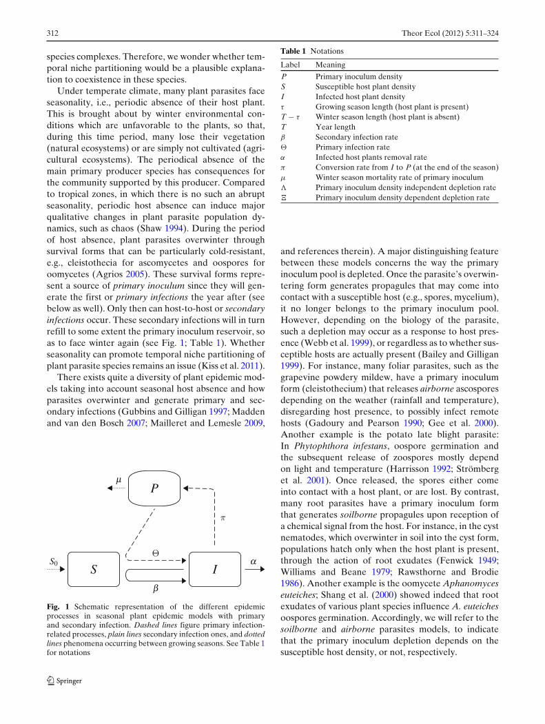
Under temperate climate, many plant parasites faceseasonality, i.e., periodic absence of their host plant.This is brought about by winter environmental con-ditions which are unfavorable to the plants, so that,during this time period, many lose their vegetation(natural ecosystems) or are simply not cultivated (agri-cultural ecosystems). The periodical absence of themain primary producer species has consequences forthe community supported by this producer. Comparedto tropical zones, in which there is no such an abruptseasonality, periodic host absence can induce majorqualitative changes in plant parasite population dy-namics, such as chaos (Shaw 1994). During the periodof host absence, plant parasites overwinter throughsurvival forms that can be particularly cold-resistant,e.g., cleistothecia for ascomycetes and oospores foroomycetes (Agrios 2005). These survival forms repre-sent a source of primary inoculum since they will gen-erate the first or primary infections the year after (seebelow as well). Only then can host-to-host or secondaryinfections occur. These secondary infections will in turnrefill to some extent the primary inoculum reservoir, soas to face winter again (see Fig. 1; Table 1). Whetherseasonality can promote temporal niche partitioning ofplant parasite species remains an issue (Kiss et al. 2011).

There exists quite a diversity of plant epidemic mod-els taking into account seasonal host absence and howparasites overwinter and generate primary and sec-ondary infections (Gubbins and Gilligan 1997; Maddenand van den Bosch 2007; Mailleret and Lemesle 2009,

Fig. 1 Schematic representation of the different epidemicprocesses in seasonal plant epidemic models with primaryand secondary infection. Dashed lines figure primary infection-related processes, plain lines secondary infection ones, and dottedlines phenomena occurring between growing seasons. See Table 1for notations

Table 1 Notations

Label Meaning

P Primary inoculum densityS Susceptible host plant densityI Infected host plant densityτ Growing season length (host plant is present)T − τ Winter season length (host plant is absent)T Year lengthβ Secondary infection rate� Primary infection rateα Infected host plants removal rateπ Conversion rate from I to P (at the end of the season)μ Winter season mortality rate of primary inoculum� Primary inoculum density independent depletion rate� Primary inoculum density dependent depletion rate

and references therein). A major distinguishing featurebetween these models concerns the way the primaryinoculum pool is depleted. Once the parasite’s overwin-tering form generates propagules that may come intocontact with a susceptible host (e.g., spores, mycelium),it no longer belongs to the primary inoculum pool.However, depending on the biology of the parasite,such a depletion may occur as a response to host pres-ence (Webb et al. 1999), or regardless as to whether sus-ceptible hosts are actually present (Bailey and Gilligan1999). For instance, many foliar parasites, such as thegrapevine powdery mildew, have a primary inoculumform (cleistothecium) that releases airborne ascosporesdepending on the weather (rainfall and temperature),disregarding host presence, to possibly infect remotehosts (Gadoury and Pearson 1990; Gee et al. 2000).Another example is the potato late blight parasite:In Phytophthora infestans, oospore germination andthe subsequent release of zoospores mostly dependon light and temperature (Harrisson 1992; Strömberget al. 2001). Once released, the spores either comeinto contact with a host plant, or are lost. By contrast,many root parasites have a primary inoculum formthat generates soilborne propagules upon reception ofa chemical signal from the host. For instance, in the cystnematodes, which overwinter in soil into the cyst form,populations hatch only when the host plant is present,through the action of root exudates (Fenwick 1949;Williams and Beane 1979; Rawsthorne and Brodie1986). Another example is the oomycete Aphanomyceseuteiches; Shang et al. (2000) showed indeed that rootexudates of various plant species influence A. euteichesoospores germination. Accordingly, we will refer to thesoilborne and airborne parasites models, to indicatethat the primary inoculum depletion depends on thesusceptible host density, or not, respectively.

Theor Ecol (2012) 5:311–324 313

Such complex biological life cycles may lead to quiteelaborate mathematical formulations (Truscott et al.1997, 2000; Madden and van den Bosch 2002). Yet,more compact and mathematically tractable forms ofseasonal plant epidemic models have recently beenproposed (Madden and van den Bosch 2007; van denBerg et al. 2011). The essential difference between theelaborate and compact models lies in the explicit ver-sus implicit nature of the primary infection modeling.Regarding coexistence of plant parasites in seasonalenvironments, van den Berg et al. (2011) showed that,in a class of compact models, a competitive exclusionprinciple holds. However, it is not clear whether thisresult holds for more elaborate models as well, e.g.,Madden and van den Bosch (2002); it may still be thatcoexistence is possible in such models. To fill this gap inour understanding of plant parasite species coexistence,we will investigate and compare airborne and soilborneparasites ecological dynamics, through reducing eachelaborate model to a mathematically more tractablecompact form. Competitive exclusion and coexistencewill then be numerically explored.

Airborne model

In this section, we consider airborne primary infec-tion dynamics. That is, we assume that primary inocu-lum depletion early in the season occurs regardless asto whether host plants are actually present (see the“Introduction”). Hence, the per day primary inoculumloss rate � will be a constant.

We build on Madden and van den Bosch (2002)’selaborate model, which explicitly considers both pri-mary and secondary infection dynamics under environ-mental seasonality. This results in a three-dimensionalsemi-discrete model (Mailleret and Lemesle 2009); twosets of ordinary differential equations, coupled to twosets of recurrence equations, define the model. Assum-ing primary infections occur on a faster time scale thansecondary infections, a slow–fast argument will showthat the three-dimensional model is approximated by atwo-dimensional semi-discrete model that is mathemat-ically more tractable. We will further analyze the lattercompact model.

Model equations

By “environmental seasonality,” we refer to the suc-cession of two time periods: the growing season, duringwhich the host plant is present, and the winter season,say, during which the host plant is absent.

We let τ be the length of the growing season andT denote the year length. Thus, (T − τ) is the winterseason length. Also, let (P, S, I) denote the primary in-oculum, susceptible host plant, and infected host plantdensities, respectively.

Let us start by considering the growing season. Asusual, β and α denote the secondary infection and theinfected host plants removal rates, respectively. Also,we let � denote the primary infection rate and � be thewithin-season primary inoculum loss rate. Thus, we letthe k-th year’s dynamics be governed by the followingequation: For t ∈ (kT, kT + τ),

P = −�P,

S = −�PS − βSI,

I = +�PS + βSI − αI, (1)

where the dot indicates derivative with respect to timet. The ±�PS terms indicate that only a fraction of thereleased primary inoculum actually encounter healthyhosts and initiate primary infection, the remaining partbeing lost (Bailey and Gilligan 1999).

At the end of the growing season (t = kT + τ ), hostplants are removed: e.g., crop plants are harvested, orleaves of deciduous trees fall down to the ground. Atthat time, infected host plants debris are assumed toconvert into primary inoculum at a rate π (the parasiteswitches to a survival form). This translates into thefollowing recurrence equation:

P(kT + τ+) = P(kT + τ) + π I(kT + τ),

S(kT + τ+) = 0,

I(kT + τ+) = 0, (2)

where the + superscript indicates the instant right afterthe end of the growing season.

During the winter season, host plants are absent andthe parasites survive as primary inoculum (P), havinga winter-specific mortality rate μ. Thus, for t ∈ (kT +τ, (k + 1)T),

P = −μP,

S = 0,

I = 0. (3)

At the beginning of a new season (t = (k + 1)T),new susceptible host plants are made available to the

314 Theor Ecol (2012) 5:311–324

parasite (crop plants are sowed or tree leaves emerge).Let their initial density be S0. This translates into

P((k + 1)T+) = P((k + 1)T),

S((k + 1)T+) = S0,

I((k + 1)T+) = 0. (4)

The semi-discrete model composed of sub-models 1to 4 thus depicts the course of an epidemic over onecycle (1 year) through primary and secondary infectiondynamics, infected host plants conversion into primaryinoculum at the end of the season, and survival tohost absence until the next year. This provides initialconditions for iterating a new cycle. It is Madden andvan den Bosch (2002)’s model.

Fast primary infections

As suggested by Madden and van den Bosch (2002),let us assume primary infections occur on a faster timescale than secondary infections. This will allow us toapproximate model 1–4 with a simpler form throughslow–fast reduction techniques commonly used in ecol-ogy (Auger et al. 2008). Mathematically, this consistsinto letting λ = ε� and θ = ε�, with 0 < ε � 1; i.e.,primary infection rate parameters � and � are assumedto take large values, compared to the secondary infec-tion parameters β and α. Using this, one can rewriteEq. 1 as

ε P = −λP,

εS = −θ PS − εβSI,ε I = +θ PS + εβSI − εαI,

(5)

with initial conditions at the beginning of year (k + 1):

P((k + 1)T+) = P((k + 1)T),

S((k + 1)T+) = S0,

I((k + 1)T+) = 0.

(6)

To take advantage of the assumption that primaryinfections are fast, i.e., that ε is small compared to 1,we now write Eq. 5 in an explicit slow–fast form. Lett′ = t/ε denote the fast time scale. After a little algebra,one gets

ddt′

(log(S) − θ

λP)

= −εβ I,

ddt′

(S + I) = −εαI,

ddt′

(P) = −λP, (7)

which is a slow–fast form of system 5 (Auger et al.2008).

The theory of slow–fast dynamical systems tells usthat, as long as ε is small, one can approximate thedynamics of system 5 by considering it on its slowmanifold only, i.e., on the subset of the state spacewhich attracts trajectories of the slow fast form of thesystem when ε is set to 0. This somehow corresponds toassuming that primary infections occur instantaneously.

For model 5, the slow manifold is determined by theattractor of Eq. 7, with ε = 0. It is thus characterizedby the fact that

(log(S) − θ

λP)

and (S + I) remain con-stant, while P goes exponentially to 0. Considering year(k + 1), the slow manifold of Eq. 5 is thus given by

P = 0,

log(S) = log(S0) − θ

λP((k + 1)T+),

S + I = S0. (8)

Using the fact that (P, S, I) belongs to the slowinvariant manifold (Eq. 8), we obtain the followingmodel:

S = −βSI,I = βSI − αI,

(9)

with initial conditions

S((k + 1)T+) = S0 exp(

−θ

λP((k + 1)T+)

),

I((k + 1)T+) = S0

(1 − exp

(−θ

λP

((k + 1)T+)))

.

(10)

(we omit P and P since both are equal to 0).

Model reduction

From Eqs. 2, 3, and 4, it is possible to further simplifyEqs. 9 and 10. It suffices to notice that Eqs. 3 and 4translate into:

P((k + 1)T+) = e−μ(T−τ) P(kT + τ+),

so that, using Eq. 2 and noticing that P(kT + τ) = 0(since the system is considered on the slow manifold(Eq. 8)), we have

P((k + 1)T+) = πe−μ(T−τ) I(kT + τ).

Using this last property in Eqs. 9 and 10, we end upwith the following compact semi-discrete model: For allk and for any t ∈ (kT, kT + τ),

S = −βSI,

I = βSI − αI,(11)

Theor Ecol (2012) 5:311–324 315

coupled to the difference equation

S((k+1)T+)= S0 exp(

−θπe−μ(T−τ)

λI(kT+τ)

),

I((k+1)T+)= S0

(1−exp

(−θπe−μ(T−τ)

λI (kT+τ)

)).

(12)

One easily sees that the compact model (Eqs. 11and 12) is well-posed: that is, it cannot produce negativetrajectories. Also, the latter remain bounded: S and Ialways remain smaller or equal to S0. It is an originalmodel (see “Linearized model” section to see how itrelates to previous compact models).

In the limit that ε tends to 0, both the elaboratemodel (Eqs. 1–4) and the compact form (Eqs. 11and 12) produce the same dynamics, while as ε remainssmall compared to 1, but not infinitely small, the com-pact form (Eqs. 11 and 12) provides a good approxima-tion of the elaborate model (Eqs. 1–4) dynamics.

Notice that, due to the fast primary infections as-sumption and other features from the elaborate model,the compact semi-discrete model is independent of P

(the primary inoculum). This reduces the dimensionof the model yet induces a time-gap during the winterseason regarding the visual output (for t ∈ (kT + τ,

(k + 1)T), the compact model shows no solution;Fig. 2.)

Linearized model

Assuming θπe−μ(T−τ)/λ is small, Eq. 12 reads:

S((k + 1)T+) ∼= S0 − θπe−μ(T−τ)

λ/S0I(kT + τ),

I((k + 1)T+) ∼= θπe−μ(T−τ)

λ/S0I(kT + τ). (13)

The linearity in the discrete part makes model 11–13essentially equivalent to Madden and van den Bosch(2007) and van den Berg et al. (2011). This shows a limitto van den Berg et al. (2011)’s result concerning the ex-istence of a competitive exclusion principle in airborneparasites which is strongly dependent on the linearityof the discrete part. It is actually unclear how smallθπe−μ(T−τ)/λ has to be (i.e., how inefficient primary

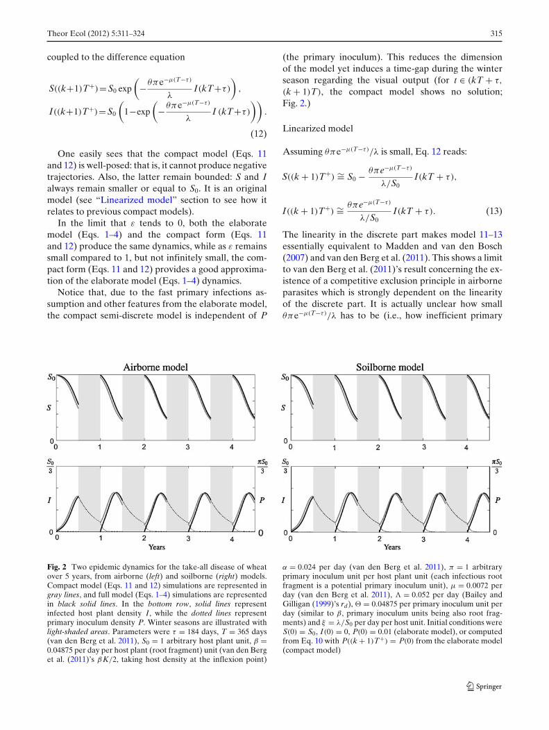
Fig. 2 Two epidemic dynamics for the take-all disease of wheatover 5 years, from airborne (left) and soilborne (right) models.Compact model (Eqs. 11 and 12) simulations are represented ingray lines, and full model (Eqs. 1–4) simulations are representedin black solid lines. In the bottom row, solid lines representinfected host plant density I, while the dotted lines representprimary inoculum density P. Winter seasons are illustrated withlight-shaded areas. Parameters were τ = 184 days, T = 365 days(van den Berg et al. 2011), S0 = 1 arbitrary host plant unit, β =0.04875 per day per host plant (root fragment) unit (van den Berget al. (2011)’s βK/2, taking host density at the inflexion point)

α = 0.024 per day (van den Berg et al. 2011), π = 1 arbitraryprimary inoculum unit per host plant unit (each infectious rootfragment is a potential primary inoculum unit), μ = 0.0072 perday (van den Berg et al. 2011), � = 0.052 per day (Bailey andGilligan (1999)’s rd), � = 0.04875 per primary inoculum unit perday (similar to β, primary inoculum units being also root frag-ments) and ξ = λ/S0 per day per host unit. Initial conditions wereS(0) = S0, I(0) = 0, P(0) = 0.01 (elaborate model), or computedfrom Eq. 10 with P((k + 1)T+) = P(0) from the elaborate model(compact model)

316 Theor Ecol (2012) 5:311–324

inoculum has to be), for the approximation 13 to remainvalid and thus for the competitive exclusion principle tohold.

R0 derivation

We define the parasite’s basic reproduction number R0

as the quantity of primary inoculum at the beginningof year (k + 1) produced via the infections generatedby one primary inoculum unit at the beginning of yeark, in a disease-free context (Diekmann and Hesterbeek2000; Madden and van den Bosch 2002, 2007; van denBosch et al. 2008). Mathematically speaking, R0 willthus be computed as P((k + 1)T+)/P(kT+) estimatedfrom the linearized dynamics around the disease-freesolution. Since winters are implicit in the compact form(Eqs. 11 and 12), the disease-free solution is actually anequilibrium and not a stationary cycle, yet it should bekept in mind that plant populations do cycle (they areabsent during winters) even though it is not apparent inthe aggregated model equations.

We now state the following result regarding thestability of the disease-free equilibrium in the compactmodel. The proof is in “Appendix 1”.

Theorem 1 The compact model (Eqs. 11 and 12) admitsa stationary disease-free solution (S, I) = (S0, 0) whichis globally asymptotically stable (GAS) if and only if theparasite’s basic reproduction number

R0 = θπe−μ(T−τ)

λe(βS0−α)τ S0,

is smaller or equal to 1.

Numerical computations

To investigate the dynamical behavior of the airbornemodel, we performed some numerical simulations ofthe elaborate and compact forms when R0 > 1. Wemost of the time identified a, seemingly GAS, periodicstationary solution of period 1 year, i.e., characterizedby the exact replication of the epidemic from one sea-son to the other. Figure 2’s left panel shows such dy-namics in which, after a transient, the epidemic reachesa periodic behavior.

Elaborate and compact models comparison

To illustrate the model reduction’s relevance, Fig. 2’sleft panel shows both the compact and elaborate modeldynamics. The parameter set was chosen to fit the take-

all disease of wheat (caused by the soilborne fungusGaeumannomyces graminis var. tritici), for which real-istic parameter values exist in the literature (Bailey andGilligan 1999; van den Berg et al. 2011). This will allowus to compare airborne and soilborne mathematicalmodels, given a parameter set.

Regarding the airborne model, even though � and �

are not that small compared to β and α (i.e., primary in-fections are not that fast), the compact model providesa good approximation of the elaborate model dynamics.

The route to chaos

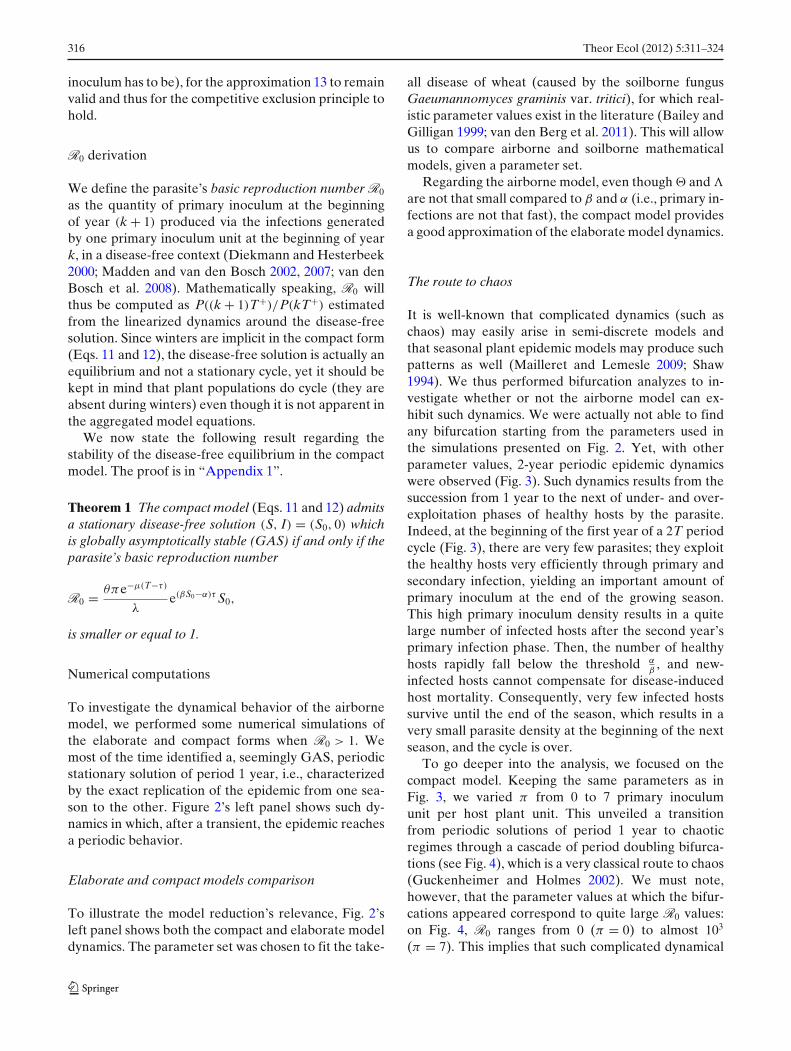
It is well-known that complicated dynamics (such aschaos) may easily arise in semi-discrete models andthat seasonal plant epidemic models may produce suchpatterns as well (Mailleret and Lemesle 2009; Shaw1994). We thus performed bifurcation analyzes to in-vestigate whether or not the airborne model can ex-hibit such dynamics. We were actually not able to findany bifurcation starting from the parameters used inthe simulations presented on Fig. 2. Yet, with otherparameter values, 2-year periodic epidemic dynamicswere observed (Fig. 3). Such dynamics results from thesuccession from 1 year to the next of under- and over-exploitation phases of healthy hosts by the parasite.Indeed, at the beginning of the first year of a 2T periodcycle (Fig. 3), there are very few parasites; they exploitthe healthy hosts very efficiently through primary andsecondary infection, yielding an important amount ofprimary inoculum at the end of the growing season.This high primary inoculum density results in a quitelarge number of infected hosts after the second year’sprimary infection phase. Then, the number of healthyhosts rapidly fall below the threshold α

β, and new-

infected hosts cannot compensate for disease-inducedhost mortality. Consequently, very few infected hostssurvive until the end of the season, which results in avery small parasite density at the beginning of the nextseason, and the cycle is over.

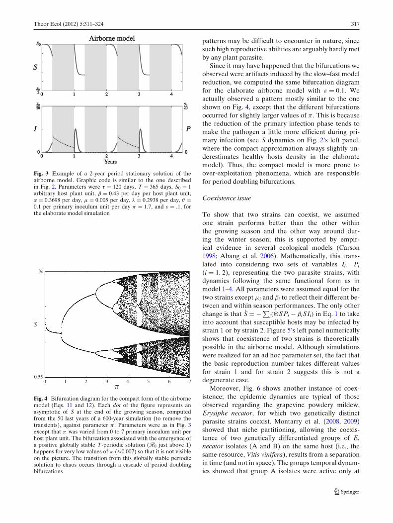
To go deeper into the analysis, we focused on thecompact model. Keeping the same parameters as inFig. 3, we varied π from 0 to 7 primary inoculumunit per host plant unit. This unveiled a transitionfrom periodic solutions of period 1 year to chaoticregimes through a cascade of period doubling bifurca-tions (see Fig. 4), which is a very classical route to chaos(Guckenheimer and Holmes 2002). We must note,however, that the parameter values at which the bifur-cations appeared correspond to quite large R0 values:on Fig. 4, R0 ranges from 0 (π = 0) to almost 103

(π = 7). This implies that such complicated dynamical

Theor Ecol (2012) 5:311–324 317

Fig. 3 Example of a 2-year period stationary solution of theairborne model. Graphic code is similar to the one describedin Fig. 2. Parameters were τ = 120 days, T = 365 days, S0 = 1arbitrary host plant unit, β = 0.43 per day per host plant unit,α = 0.3698 per day, μ = 0.005 per day, λ = 0.2938 per day, θ =0.1 per primary inoculum unit per day π = 1.7, and ε = .1, forthe elaborate model simulation

Fig. 4 Bifurcation diagram for the compact form of the airbornemodel (Eqs. 11 and 12). Each dot of the figure represents anasymptotic of S at the end of the growing season, computedfrom the 50 last years of a 600-year simulation (to remove thetransients), against parameter π . Parameters were as in Fig. 3except that π was varied from 0 to 7 primary inoculum unit perhost plant unit. The bifurcation associated with the emergence ofa positive globally stable T-periodic solution (R0 just above 1)happens for very low values of π (≈0.007) so that it is not visibleon the picture. The transition from this globally stable periodicsolution to chaos occurs through a cascade of period doublingbifurcations

patterns may be difficult to encounter in nature, sincesuch high reproductive abilities are arguably hardly metby any plant parasite.

Since it may have happened that the bifurcations weobserved were artifacts induced by the slow–fast modelreduction, we computed the same bifurcation diagramfor the elaborate airborne model with ε = 0.1. Weactually observed a pattern mostly similar to the oneshown on Fig. 4, except that the different bifurcationsoccurred for slightly larger values of π . This is becausethe reduction of the primary infection phase tends tomake the pathogen a little more efficient during pri-mary infection (see S dynamics on Fig. 2’s left panel,where the compact approximation always slightly un-derestimates healthy hosts density in the elaboratemodel). Thus, the compact model is more prone toover-exploitation phenomena, which are responsiblefor period doubling bifurcations.

Coexistence issue

To show that two strains can coexist, we assumedone strain performs better than the other withinthe growing season and the other way around dur-ing the winter season; this is supported by empir-ical evidence in several ecological models (Carson1998; Abang et al. 2006). Mathematically, this trans-lated into considering two sets of variables Ii, Pi

(i = 1, 2), representing the two parasite strains, withdynamics following the same functional form as inmodel 1–4. All parameters were assumed equal for thetwo strains except μi and βi to reflect their different be-tween and within season performances. The only otherchange is that S = − ∑

i(�SPi − βiSIi) in Eq. 1 to takeinto account that susceptible hosts may be infected bystrain 1 or by strain 2. Figure 5’s left panel numericallyshows that coexistence of two strains is theoreticallypossible in the airborne model. Although simulationswere realized for an ad hoc parameter set, the fact thatthe basic reproduction number takes different valuesfor strain 1 and for strain 2 suggests this is not adegenerate case.

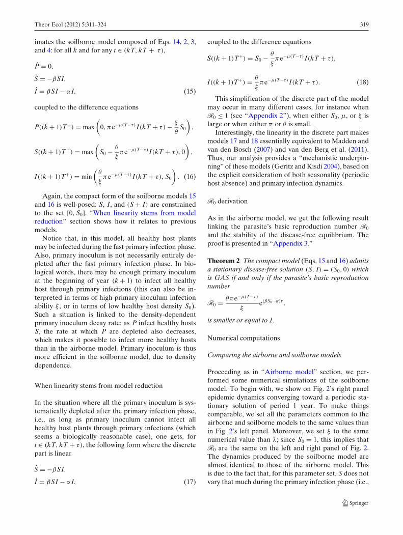
Moreover, Fig. 6 shows another instance of coex-istence; the epidemic dynamics are typical of thoseobserved regarding the grapevine powdery mildew,Erysiphe necator, for which two genetically distinctparasite strains coexist. Montarry et al. (2008, 2009)showed that niche partitioning, allowing the coexis-tence of two genetically differentiated groups of E.necator isolates (A and B) on the same host (i.e., thesame resource, Vitis vinifera), results from a separationin time (and not in space). The groups temporal dynam-ics showed that group A isolates were active only at

318 Theor Ecol (2012) 5:311–324

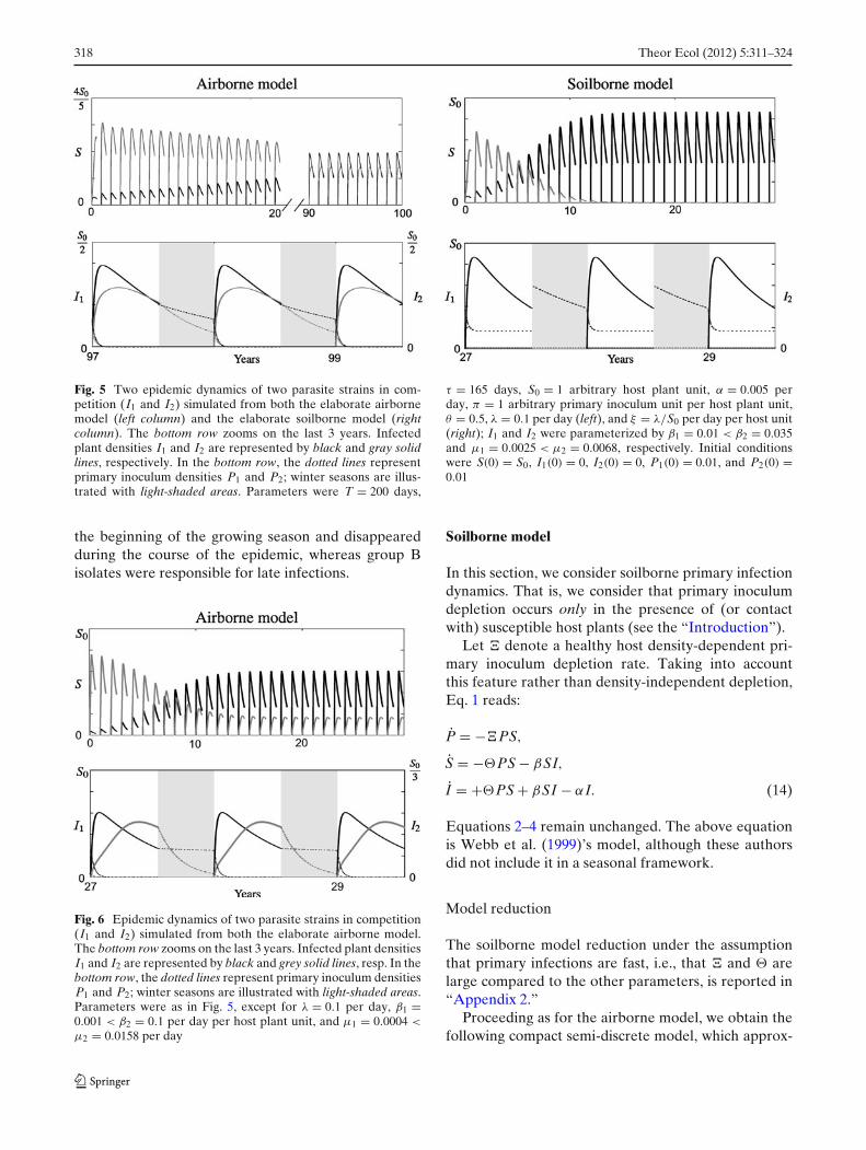
Fig. 5 Two epidemic dynamics of two parasite strains in com-petition (I1 and I2) simulated from both the elaborate airbornemodel (left column) and the elaborate soilborne model (rightcolumn). The bottom row zooms on the last 3 years. Infectedplant densities I1 and I2 are represented by black and gray solidlines, respectively. In the bottom row, the dotted lines representprimary inoculum densities P1 and P2; winter seasons are illus-trated with light-shaded areas. Parameters were T = 200 days,

τ = 165 days, S0 = 1 arbitrary host plant unit, α = 0.005 perday, π = 1 arbitrary primary inoculum unit per host plant unit,θ = 0.5, λ = 0.1 per day (left), and ξ = λ/S0 per day per host unit(right); I1 and I2 were parameterized by β1 = 0.01 < β2 = 0.035and μ1 = 0.0025 < μ2 = 0.0068, respectively. Initial conditionswere S(0) = S0, I1(0) = 0, I2(0) = 0, P1(0) = 0.01, and P2(0) =0.01

the beginning of the growing season and disappearedduring the course of the epidemic, whereas group Bisolates were responsible for late infections.

Fig. 6 Epidemic dynamics of two parasite strains in competition(I1 and I2) simulated from both the elaborate airborne model.The bottom row zooms on the last 3 years. Infected plant densitiesI1 and I2 are represented by black and grey solid lines, resp. In thebottom row, the dotted lines represent primary inoculum densitiesP1 and P2; winter seasons are illustrated with light-shaded areas.Parameters were as in Fig. 5, except for λ = 0.1 per day, β1 =0.001 < β2 = 0.1 per day per host plant unit, and μ1 = 0.0004 <

μ2 = 0.0158 per day

Soilborne model

In this section, we consider soilborne primary infectiondynamics. That is, we consider that primary inoculumdepletion occurs only in the presence of (or contactwith) susceptible host plants (see the “Introduction”).

Let � denote a healthy host density-dependent pri-mary inoculum depletion rate. Taking into accountthis feature rather than density-independent depletion,Eq. 1 reads:

P = −�PS,

S = −�PS − βSI,

I = +�PS + βSI − αI. (14)

Equations 2–4 remain unchanged. The above equationis Webb et al. (1999)’s model, although these authorsdid not include it in a seasonal framework.

Model reduction

The soilborne model reduction under the assumptionthat primary infections are fast, i.e., that � and � arelarge compared to the other parameters, is reported in“Appendix 2.”

Proceeding as for the airborne model, we obtain thefollowing compact semi-discrete model, which approx-

Theor Ecol (2012) 5:311–324 319

imates the soilborne model composed of Eqs. 14, 2, 3,and 4: for all k and for any t ∈ (kT, kT + τ),

P = 0,

S = −βSI,

I = βSI − αI, (15)

coupled to the difference equations

P((k + 1)T+) = max(

0, πe−μ(T−τ) I(kT + τ) − ξ

θS0

),

S((k + 1)T+) = max(

S0 − θ

ξπe−μ(T−τ) I(kT + τ), 0

),

I((k + 1)T+) = min(

θ

ξπe−μ(T−τ) I(kT + τ), S0

). (16)

Again, the compact form of the soilborne models 15and 16 is well-posed: S, I, and (S + I) are constrainedto the set [0, S0]. “When linearity stems from modelreduction” section shows how it relates to previousmodels.

Notice that, in this model, all healthy host plantsmay be infected during the fast primary infection phase.Also, primary inoculum is not necessarily entirely de-pleted after the fast primary infection phase. In bio-logical words, there may be enough primary inoculumat the beginning of year (k + 1) to infect all healthyhost through primary infections (this can also be in-terpreted in terms of high primary inoculum infectionability ξ , or in terms of low healthy host density S0).Such a situation is linked to the density-dependentprimary inoculum decay rate: as P infect healthy hostsS, the rate at which P are depleted also decreases,which makes it possible to infect more healthy hoststhan in the airborne model. Primary inoculum is thusmore efficient in the soilborne model, due to densitydependence.

When linearity stems from model reduction

In the situation where all the primary inoculum is sys-tematically depleted after the primary infection phase,i.e., as long as primary inoculum cannot infect allhealthy host plants through primary infections (whichseems a biologically reasonable case), one gets, fort ∈ (kT, kT + τ), the following form where the discretepart is linear

S = −βSI,

I = βSI − αI, (17)

coupled to the difference equations

S((k + 1)T+) = S0 − θ

ξπe−μ(T−τ) I(kT + τ),

I((k + 1)T+) = θ

ξπe−μ(T−τ) I(kT + τ). (18)

This simplification of the discrete part of the modelmay occur in many different cases, for instance whenR0 ≤ 1 (see “Appendix 2”), when either S0, μ, or ξ islarge or when either π or θ is small.

Interestingly, the linearity in the discrete part makesmodels 17 and 18 essentially equivalent to Madden andvan den Bosch (2007) and van den Berg et al. (2011).Thus, our analysis provides a “mechanistic underpin-ning” of these models (Geritz and Kisdi 2004), based onthe explicit consideration of both seasonality (periodichost absence) and primary infection dynamics.

R0 derivation

As in the airborne model, we get the following resultlinking the parasite’s basic reproduction number R0

and the stability of the disease-free equilibrium. Theproof is presented in “Appendix 3.”

Theorem 2 The compact model (Eqs. 15 and 16) admitsa stationary disease-free solution (S, I) = (S0, 0) whichis GAS if and only if the parasite’s basic reproductionnumber

R0 = θπe−μ(T−τ)

ξe(βS0−α)τ .

is smaller or equal to 1.

Numerical computations

Comparing the airborne and soilborne models

Proceeding as in “Airborne model” section, we per-formed some numerical simulations of the soilbornemodel. To begin with, we show on Fig. 2’s right panelepidemic dynamics converging toward a periodic sta-tionary solution of period 1 year. To make thingscomparable, we set all the parameters common to theairborne and soilborne models to the same values thanin Fig. 2’s left panel. Moreover, we set ξ to the samenumerical value than λ; since S0 = 1, this implies thatR0 are the same on the left and right panel of Fig. 2.The dynamics produced by the soilborne model arealmost identical to those of the airborne model. Thisis due to the fact that, for this parameter set, S does notvary that much during the primary infection phase (i.e.,

320 Theor Ecol (2012) 5:311–324

ξ S ≈ ξ S0 = λ), making density dependence apparentlytransparent.

Regarding chaos

We also proceeded to a bifurcation analysis for thecompact form of the soilborne model, once againchoosing the same parameter values than for the air-borne model and letting ξ being equal to the numer-ical value of λ for the airborne model (Fig. 4), whichresulted in comparing models with the same R0. Weobtained a bifurcation diagram very similar to the air-borne model’s one (Fig. 4), except that the bifurcationoccurred for slightly lower values of the parameter π .This is caused by primary inoculum being more efficientin the soilborne model, which renders the system moreprone to over-exploitation phenomena and thus to bi-furcations (“The route to chaos” section). Again, asfor the airborne model, we observed the same bifur-cation diagram for the elaborate form of the soilbornemodel with ε = 0.1, except that bifurcations occurredfor slightly larger values of the parameter π .

Coexistence issue

To investigate the two-strain dynamics, we proceededas for the airborne model, regarding the two-strainmodel. Figure 5’s right panel numerically illustratesthe competitive exclusion principle van den Berg et al.(2011) found regarding the compact form of the model,by showing that it holds in the associated soilborneelaborate model. However, one sees that this doesnot hold anymore in the airborne model (Fig. 5’s leftpanel), everything else being unchanged. Therefore,although Fig. 2 indicates that there is little quantitativedifference in the take-all disease dynamics between air-borne and soilborne models, the structural differencesarise when looking at the qualitative dynamics in abroader ecological context. In other words, our studyshows that density dependence in the primary inoculumdepletion rate, which is typical of soilborne diseases,may prevent species coexistence.

Discussion

Two three-dimensional semi-discrete models, named“airborne” and “soilborne” models, were investigated.Both models combine seasonality (periodic host ab-sence) and explicit primary infection dynamics, as inMadden and van den Bosch (2002). Airborne andsoilborne models differ in that the primary inocu-lum depletion rate is density independent and depen-

dent, respectively (Webb et al. 1999). Assuming pri-mary infections are fast, reduction techniques (Augeret al. 2008) allowed us to derive two two-dimensionalmodel approximations that are mathematically moretractable.

A first issue was whether one recovers a simple semi-discrete model whose continuous part is the standardSIR model (Smith 2008) and whose discrete part islinear, as in Madden and van den Bosch (2007) andvan den Berg et al. (2011). One ecological implicationcomes from the fact that the latter authors showed acompetitive exclusion principle holds in such a model.That is, the parasite strain having the largest epi-demiological basic reproduction number R0, definedin “Appendix 4”, eventually wins the competition; theother strains die out. Long run coexistence is thusimpossible in such a model.

In both airborne and soilborne models, applying theaforementioned reduction technique led to a continu-ous SIR part, yet to a generally nonlinear discrete part.Regarding the airborne model, “Linearized model”section showed that it can be linearized in the limitof an infinitely small composite parameter. As for thesoilborne model, “When linearity stems from modelreduction” section showed that it simplifies to a lineardiscrete part very similar to Madden and van den Bosch(2007) and van den Berg et al. (2011) in a significantpart of the parameter space.

On the one hand, this indicates that long-run persis-tence is unlikely in the soilborne model. Yet, there isno lack of empirical counterexamples, e.g., for the take-all disease of wheat (Lebreton et al. 2007; Daval et al.2010). A simple explanation to that apparent paradox isthat G. graminis var. tritici, although being a soilborneplant parasite, better fits the airborne model because itreleases propagules (free-living mycelium, which growsin the soil) regardless of host (wheat roots) presence(Bailey and Gilligan 1999). This allows us to stress thatthe so named airborne and soilborne models do notnecessarily correspond to the biologically very diverseairborne and soilborne plant parasites, respectively.

On the other hand, we numerically showed that longrun coexistence is possible in the airborne model. Thisis supported by experimental evidence, such as withinthe powdery mildew species complex (“Coexistenceissue” section). The theoretical investigation of theevolution of plant parasites in seasonal environments iscurrently receiving increased attention (van den Berget al. 2010, 2011). Yet these studies are based on epi-demic models in which a competitive exclusion prin-ciple holds, what tremendously restricts the possibleoutcomes of natural selection. Future research shouldthus address the evolutionary implications of systems

Theor Ecol (2012) 5:311–324 321

allowing more complex behaviors, such as co-existenceof different parasite species, like, e.g., in the presentairborne model.

Acknowledgements This research was supported by grantsfrom Agropolis Fondation and RNSC (covenant support number0902-013) and from INRA (call for proposal “Gestion durabledes résistances aux bio-agresseurs,” contract number 394576).MC is supported by a Ph.D. grant from the INRA SPE De-partment and the Région Bretagne. This work is part of anINRA-BBSRC funded project entitled “Epidemiological andevolutionary models for invasion and persistence of plant dis-eases.” We are grateful to an anonymous reviewer for insightfulcomments on the paper.

Appendix 1: Proof of theorem 1

It is easy to see that (S, I) = (S0, 0) is a stationarysolution of Eq. 11, so that I(kT + τ) = 0, which usedin Eq. 12, implies that at the beginning of year (k + 1),S((k + 1)T+) = S0 and I((k + 1)T+) = 0. Therefore,the disease-free solution (S, I) = (S0, 0) is an equilib-rium of models 11 and 12.

Linearizing Eqs. 11 and 12 around (S, I) = (S0, 0),yields

I(kT + τ) = e(βS0−α)τ I(kT+),

= e(βS0−α)τ S0θπe−μ(T−τ)

λI((k − 1)T + τ),

so that, remembering that P((k+1)T+)=πe−μ(T−τ)I(kT+τ)

and rearranging the terms, we get

R0 = P((k + 1)T+)

P(kT+)= θπe−μ(T−τ)

λe(βS0−α)τ S0.

Consider Eq. 11. Since S is always upper-bounded byS0, we have, for t ∈ (kT, kT + τ),

I ≤ (βS0 − α)I ⇒ I(kT + τ) ≤ e(βS0−α)τ I(kT+),

so that, using Eq. 12, we have:

I((k + 1)T+)

≤ S0

(1 − exp

(−θπe−μ(T−τ)

λe(βS0−α)τ I(kT+)

)).

The right-hand side of the previous equation is anincreasing, strictly concave, function of I(kT+) whichequals 0 for I(kT+) = 0 with a slope equal to

S0θπe−μ(T−τ)

λe(βS0−α)τ = R0

around I(kT+) = 0. Classical results on one-dimensional recurrence equations allows one to

conclude that if R0 is smaller or equal to 1, thesequence (I(kT+))k∈N is decreasing and converges to 0as k goes to infinity.

A similar argument can be used for the sequence(S0 − S(kT+))k∈N, showing that, if R0 ≤ 1, the se-quence (S(kT+))k∈N is increasing and converges to S0

as k goes to infinity. Thus, the disease-free solution(S0, 0) is globally attractive provided R0 ≤ 1. On onehand, the monotonicity of both sequences (I(kT+))k∈N

and (S(kT+))k∈N also implies that (S0, 0) is locally sta-ble if R0 ≤ 1. On the other hand, the considerationof models 11 and 12 linearized around (S0, 0) easilyallows one to conclude that the disease-free solution isunstable if R0 > 1. This concludes the proof that (S0, 0)

is GAS if and only if R0 ≤ 1.

Appendix 2: Fast primary infections in the soilbornemodel

Proceeding as for the airborne model, let ξ = ε�. Equa-tion 14 reads, in an explicit slow–fast form:

ddt′

(S − θ

ξP)

= −εβSI,

ddt′

(S + I) = −εαI,

ddt′

(P) = −ξ P((

S − θ

ξP)

+ θ

ξP)

. (19)

Thus, the slow manifold of system 19 is characterized

by the fact that(

S − θξ

P)

and (S + I) remain constant.During year (k + 1), according to Eq. 4, these con-

stants are equal to(

S0 − θξ

P((k + 1)T+))

and S0, re-spectively. Taking this into account and letting ε tend to0, we get that the fast dynamics of P are determined by:

ddt′

(P) = −P((

ξ S0 − θ P((k + 1)T+)) + θ P

), (20)

which is a quadratic differential equation with twoequilibria

P1 = 0, and P2 = P((k + 1)T+) − ξ

θS0,

the latter being positive or negative depending on S0,ξ , θ , and P((k + 1)T+). Actually, the sign of P2 alsodetermines which equilibrium is an attractor.

322 Theor Ecol (2012) 5:311–324

If P2 ≤ 0, P1 = 0 is an attractor of the fast Eq. 20 forpositive initial conditions, the slow manifold reduces tothe set

P = 0,

S = S0 − θ

ξP((k + 1)T+),

I = θ

ξP((k + 1)T+).

If P2 > 0, then P2 = (P((k + 1)T+) − ξ

θS0

)is an at-

tractor of the fast Eq. 20 for positive initial conditions.In that case, the slow manifold of Eq. 19 is the set

P =(

P((k + 1)T+) − ξ

θS0

),

S = 0,

I = S0.

It is actually possible to summarize these two casesusing the max and min functions. One obtains that theslow manifold of system 19 is the set

P = max(

0, P((k + 1)T+) − ξ

θS0

),

S = max(

S0 − θ

ξP((k + 1)T+), 0

),

I = min(

θ

ξP((k + 1)T+), S0

). (21)

In these notations, either P, S, and I are all equal to thefirst argument of the functions max or min, respectively,or are all equal to the second.

Appendix 3: Proof of theorem 2

We compute the basic reproduction number in models15 and 16 from the linearization of the model aroundthe disease-free equilibrium (S0, 0); we easily obtain

R0 = P((k + 1)T+)

P(kT+)= θπe−μ(T−τ)

ξe(βS0−α)τ .

As in the airborne model, it is fairly easy to show that(S0, 0) is a stationary solution of models 15 and 16.

Consider I in Eq. 15. Remembering that (S + I) isrestricted to [0, S0], we have ∀t ∈ (kT, kT + τ),

I ≤ β(S0 − I)I − αI = (βS0 − α)

(1 − β I

βS0 − α

)I,

Exploiting order preserving flow properties of one-dimensional ordinary differential equations and sepa-ration of variables techniques, we get

I(kT + τ) ≤ (βS0 − α)e(βS0−α)τ I(kT+)

(βS0 − α) + β(e(βS0−α)τ − 1)I(kT+).

(22)

We shall now use the third equation in Eq. 16 tocompute I((k + 1)T+), but the nonlinear min functionrequires some attention. One can easily show thatI(kT + τ) ≤ e(βS0−α)τ S0. Thus

θ

ξπe−μ(T−τ) I(kT+τ)≤ θ

ξπe−μ(T−τ)e(βS0−α)τ S0 =R0S0,

so that if R0 ≤ 1, we have

min(

θ

ξπe−μ(T−τ) I(kT+τ), S0

)= θ

ξπe−μ(T−τ) I(kT+τ).

Assume from now on R0 ≤ 1. Using Eq. 22 and theprevious remark, we get

I((k + 1)T+) ≤θξπe−μ(T−τ)(βS0 − α)e(βS0−α)τ I(kT+)

(βS0 − α) + β(e(βS0−α)τ − 1)I(kT+).

As in “Appendix 1” the right-hand side of the previousequation is an increasing, strictly concave, function ofI(kT+) which equals 0 for I(kT+) = 0 with a slopeequal to

θπe−μ(T−τ)

ξe(βS0−α)τ = R0

at I(kT+) = 0. Concluding that (S0, 0) is globally at-tractive for trajectories of models 15 and 16 if R0 ≤ 1is no harder than in the airborne case, nor is the local(un)stability study.

Appendix 4: Alternate R0 definition and evolutionaryimplications

Using a technique introduced by Bacaer andGuernaoui (2006) to study periodic epidemic models,the parasite’s basic reproductive number can bederived alternately. Let us focus on the airbornemodel. A similar derivation can be made regardingthe soilborne model, mutatis mutandis. Let us linearizeEqs. 11 and 12 around the disease-free equilibrium(S0, 0) at first order in s and i, with (S, I) = (S0 + s, i).Since for all t ∈ (kT + τ, (k + 1)T) models 11 and 12define no solution (the time-gap mentioned in the bodyof the paper), we find convenient to make the following

Theor Ecol (2012) 5:311–324 323

time change: Let z = t − (k − 1)(T − τ), with k ∈ N∗.

We get, for the continuous part: ∀z ∈ [kτ, (k + 1)τ ),

didz

= (βS0 − α)i , (23)

and for the discrete part: ∀k ∈ N∗,

i(kτ+) = S0

(1 − exp

(−θπe−μ(T−τ)

λi(kτ)

))

∼= S0θπe−μ(T−τ)

λi(kτ) , (24)

since i is assumed to be small. Proceeding as in van denBerg et al. (2011), Eqs. 23 and 24 also read:

didz

=(

βS0 − α + log(

θπe−μ(T−τ)

λS0

)δ(t − kτ)

)i ,

(25)

where δ is Dirac’s delta function. Bacaer andGuernaoui (2006) showed that for a system such asEq. 25, one obtains a basic reproduction number de-noted R0 such as:

R0 =

⎧⎪⎪⎪⎪⎪⎪⎪⎪⎪⎪⎪⎨⎪⎪⎪⎪⎪⎪⎪⎪⎪⎪⎪⎩

βS0τ

ατ −log(θπe−μ(T−τ)

λS0

) ifθπe−μ(T−τ)

λS0 <1,

βS0

αif

θπe−μ(T−τ)

λS0 =1,

βS0τ +log(θπe−μ(T−τ)

λS0

)

ατif

θπe−μ(T−τ)

λS0 >1.

(26)

Notice that R0 > 1 ⇔ R0 > 1. The difference is a mat-ter of definition. In the body of the paper, we showedthat R0 is the basic reproduction number of a primaryinoculum unit. In other words, R0 is an ecologicaldefinition. R0 is rather an epidemiological definition: Itis the expected number of infections directly generatedby a single infected individual introduced at a randomtime, in a disease-free context.

Interestingly, “Linearized model” section and vanden Berg et al. (2011) strongly suggest that in the limitof infinitely small values of θπe−μ(T−τ)/λ, the strainthat has the greatest epidemiological R0 (rather thanthe largest ecological R0) is expected to eventually winthe competition. See, e.g., (Mylius and Diekmann 1995)for related issues in a broader ecological context.

References

Abang MM, Baum M, Ceccarelli S, Grando S, Linde CC,Yahyaoui A, Zhan J, McDonald BA (2006) Differentialselection on Rhynchosporium secalis during parasitic andsaprophytic phases in the barley scald disease cycle. Phy-topathology 96:1214–1222

Agrios G (2005) Plant pathology. Elsevier Academic, San DiegoAmarasekare, P (2003) Competitive coexistence in spatially

structured environments: a synthesis. Ecol Lett 6:1109–1122Auger P, Bravo de la Parra R, Poggiale JC, Sánchez E (2008)

Aggregation methods in dynamical systems and applicationsin population and community dynamics. Phys Life Rev 5:79–105

Bacaer N, Guernaoui S (2006) The epidemic threshold of vector-borne diseases with seasonality. J Math Biol 53(3):421–436

Bailey DJ, Gilligan CA (1999). Dynamics of primary andsecondary infection in take-all epidemics. Phytopathology89:84–91

Carson ML (1998) Aggressiveness and perennation of isolates ofCochliobolus heterostrophus from North Carolina. Plant Dis82:1043–1047

Chesson, P (2000) Mechanisms of maintenance of species diver-sity. Annu Rev Ecol Syst 31:343–366

Daval S, Lebreton L, Gazengel K, Guillerm-Erckelboudt AY,Sarniguet A (2010) Genetic evidence for differentiation ofGaeumannomyces graminis var. tritici into two major groups.Plant Pathol 59:165–178

Diekmann O, Hesterbeek JAP (2000) Mathematical epidemiol-ogy of infectious diseases: model building, analysis and inter-pretation. Wiley, Chichester

Fenwick DW (1949) Investigations on the emergence of lar-vae from cysts of the potato-root eelworm Heteroderarostochiensis. I. Technique and variability. J Helminthol23:157–170

Fitt BDL, Huang YJ, van den Bosch F, West JS (2006) Coexis-tence of related pathogen species on arable crops in spaceand time. Annu Rev Phytopathol 44:163–182

Fournier E, Giraud T (2008) Sympatric genetic differentiationof populations of a generalist pathogenic fungus, Botrytiscinerea, on two different host plants, grapevine and bramble.J Evol Biol 21:122–132

Gadoury DM, Pearson RC (1990) Ascocarp dehiscence andascospore discharge in Uncinula necator. Phytopathology80:393–401

Gause, GF (1934) The struggle for existence. Williams andWilkins, Baltimore

Gee LM, Stummer BE, Gadoury DM, Biggins LT, Scott ES(2000) Maturation of cleistothecia of Uncinula necator(powdery mildew) and release of ascospores in southernAustralia. Aust J Grape Wine Res 6:13–20

Geritz SAH, Kisdi E (2004) On the mechanistic underpinning ofdiscrete time population models with complex dynamics. JTheor Biol 228:261–269

Gubbins S, Gilligan CA (1997) Persistence of host-parasite inter-actions in a disturbed environment. J Theor Biol 188(2):241–258

Guckenheimer J, Holmes P (2002) Nonlinear oscillations, dy-namical systems, and bifurcations of vector fields, appliedmathematical sciences, vol 42. Springer, New York

Harrison JG (1992) Effects of the aerial environment on lateblight of potato foliage—a review. Plant Pathol 41:384–416

Kiss L, Pintye A, Kovács GM, Jankovics T, Fontaine MC,Harvey N, Xu X, Nicot PC, Bardin M, Shykoff JA,Giraud T (2011) Temporal isolation explains host-related

324 Theor Ecol (2012) 5:311–324

genetic differentiation in a group of widespread mycopara-sitic fungi. Mol Ecol 20:1492–1507. doi:10.1111/j.1365-294X.2011.05007.x

Lebreton L, Gosme M, Lucas P, Guillerm-Erckelboudt AY,Sarniguet A (2007) Linear relationship between Gaeuman-nomyces graminis var. tritici (Ggt) genotypic frequencies anddisease severity on wheat roots in the field. Environ Micro-biol 9:492–499

Madden LV, van den Bosch F (2002) A population-dynamicsapproach to assess the threat of plant pathogens as bio-logical weapons against annual crops. BioScience 52(1):65–74

Madden LV, van den Bosch F (2007) The study of plant diseasesepidemics. APS, Saint Paul

Mailleret L, Lemesle V (2009) A note on semi-discrete mod-elling in the life sciences. Philos Trans R Soc A 367:4779–4799

Montarry J, Cartolaro P, Delmotte F, Jolivet J, Willocquet L(2008) Genetic structure and aggressiveness of Erysiphenecator populations during grapevine powdery mildew epi-demics. Appl Environ Microbiol 74:6327–6332

Montarry J, Cartolaro P, Richard-Cervera S, Delmotte F (2009)Spatio-temporal distribution of Erysiphe necator geneticgroups and their relationship with disease level in vineyards.Eur J Plant Pathol 123:61–70

Mougou A, Dutech C, Desprez-Loustau ML (2008) New insightsinto the identity and origin of the causal agent of oak pow-dery mildew in Europe. For Pathol 38:275–287

Mougou Hamdane A, Giresse X, Dutech C, Desprez-LoustauML (2010) Spatial distribution of lineages of oak powderymildew fungi in France, using quick molecular detectionmethods. Ann For Sci. doi:10.1051/forest/2009105

Mylius SD, Diekmann O (1995) On evolutionarily stable life his-tories, optimization and the need to be specific about densitydependence. Oikos 74:218–224

Rawsthorne D, Brodie B (1986) Root growth of susceptibleand resistant potato cultivars and population dynamics ofGlobodera rostochiensis in the field. J Nematol 18:379–384

Shang H, Grau CR, Peters RD (2000) Oospore germination ofAphanomyces euteiches in root exudates and on the rhizo-planes of crop plants. Plant Dis 84:994–998

Shaw MW (1994) Seasonally induced chaotic dynamics andtheir implications in models of plant disease. Plant Pathol43(5):790–801

Smith, RJ (2008) Modelling disease ecology with mathematics.American Institute of Mathematical Sciences, Springfield

Strömberg A, Boström U, Hallenberg, N (2001) Oospore germi-nation and formation by late blight pathogen Phytophthorainfestans in vitro and under field conditions. J Phytopathol149:659–664

Truscott JE, Webb CR, Gilligan CA (1997) Asymptotic analysisof an epidemic model with primary and secondary infection.Bull Math Biol 59(6):1101–1123

Truscott JE, Gilligan CA, Webb CR (2000) Quantitative analysisand model simplification of an epidemic model with primaryand secondary infection. Bull Math Biol 62(2):377–393

van den Bosch F, McRoberts N, van den Berg F, Madden LV(2008) The basic reproduction number of plant pathogens:matrix approaches to complex dynamics. Phytopathology98(2):239–249

van den Berg F, Gilligan CA, Bailey DJ, van den Bosch F (2010)Periodicity in host availability does not account for evolu-tionary branching as observed in many plant pathogens: anapplication to Gaeumannomyces graminis var. tritici. Phy-topathology 100:1169–1175

van den Berg F, Bacaer N, Metz JAJ, Lannou C, van den BoschF (2011) Periodic host absence can select for both higher orlower parasite transmission rates. Evol Ecol 25(1):121–137

Webb CR, Gilligan CA, Asher MJC (1999) A model for the tem-poral buildup of Polymyxa betae. Phytopathology 89(1):30–38

Williams T, Beane J (1979) Temperature and root exudates onthe cereal cyst-nematode Heterodera avenae. Nematologica25:397–405

Wilson M and Lindow SE (1994) Coexistence among epiphyticbacterial populations mediated through nutritional resourcepartitioning. Appl Environ Microbiol 60:4468–4477