Embed Size (px)
Citation preview
From Ideas to Trade
Carolina Ines Pan∗ and Fernando Yu†
Preliminary and Incomplete
Abstract
This paper studies how cross-country differences in the allocation of technology
affect bilateral trade. Do both the stock and dispersion of technology matter for ex-
ports? We build on Eaton and Kortum (2002) and develop a Ricardian model where
the process of innovation determines both the stock and dispersion of technology in
each country. Like in the EK model, a higher stock of technology and lower relative
input costs foster exports. Unlike in the EK model, a country’s overall comparative
advantage depends on the country-specific dispersion of technology which governs the
advantage of having lower input costs. In particular, a smaller technological dispersion
benefits countries with lower input costs since trade is determined by these and not
technological differences. The opposite is true for a high dispersion. To test our model
we create a novel dataset of historical patents and use these to construct our technology
variables. Our results confirm our model’s predictions and indicate that technological
innovation matters for trade through both the stock of patents and their dispersion
across the economy.
Keywords: Ricardian model, Comparative advantage, Technology, Patents
JEL Classification: F10, F11, O31
∗Brandeis University, International Business School, Mailstop 32 Waltham, MA (02454). E-mail:
[email protected]†Harvard University, Department of Economics: Littauer Center, 1805 Cambridge Street, Cambridge,
MA (02138). E-mail: [email protected]
1
1 Introduction
One of the oldest and most well known theories of international trade, the Ricardian theory,
highlights the role of technological dispersion as the key driver of bilateral trade. Differences
in technological capabilities across sectors and across countries determine who exports which
good. Countries will benefit by specializing in those goods in which they have a comparative
advantage and exchanging them for the other goods. Eaton and Kortum (2002), henceforth
EK, develops a general equilibrium model that extends the Ricardian framework to many
countries and many goods, capturing how the opposing forces of technology and geographic
barriers affect bilateral trade. This seminal model, however, assumes that technological
dispersion is the same for every country. In essence, this means that either all countries in
the world are technologically diversified across their industries or they are all specialized,
but we cannot have both. In this paper we show that technological dispersion indeed varies
substantially across countries, and that this variation plays an important role in bilateral
trade.
Figure 1 showcases our main argument by providing evidence that technology and trade
are related in both the first and second moments. The left panel plots the the share of world
technology, measured by patents, against the share of world exports for many countries and
years. Each dot represents a country-year, from a pool of 84 countries over the period 1985-
2000. This positive association between the stock of technology and trade is not surprising at
all and is embedded in most models of trade an innovation1. The right panel of Figure 1, on
the other hand, reveals two new stylized facts in the trade literature that served to motivate
our work: that dispersion in patenting activities (technology) varies across countries and
years, and that it is highly correlated with bilateral trade. In particular, using the familiar
1Models that explain the role of technology in trade, like EK, predict that countries with a higher stock
of technology will export more. In addition, studies about the role of international trade in innovation,
show that both higher exports (through larger markets, see Lileeva and Trefler (2010) and Bustos (2011))
and imports (through increased competition, see Bloom, Draca, and Van Reenen (2015) and Steinwender
(2015)) lead to higher innovation. Therefore, both channels predict a positive correlation between the stock
of technology and trade.
2
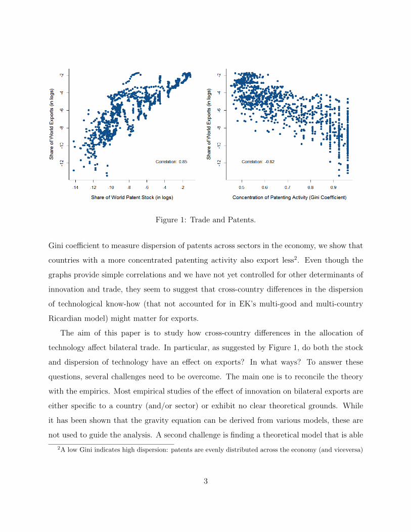
Figure 1: Trade and Patents.
Gini coefficient to measure dispersion of patents across sectors in the economy, we show that
countries with a more concentrated patenting activity also export less2. Even though the
graphs provide simple correlations and we have not yet controlled for other determinants of
innovation and trade, they seem to suggest that cross-country differences in the dispersion
of technological know-how (that not accounted for in EK’s multi-good and multi-country
Ricardian model) might matter for exports.
The aim of this paper is to study how cross-country differences in the allocation of
technology affect bilateral trade. In particular, as suggested by Figure 1, do both the stock
and dispersion of technology have an effect on exports? In what ways? To answer these
questions, several challenges need to be overcome. The main one is to reconcile the theory
with the empirics. Most empirical studies of the effect of innovation on bilateral exports are
either specific to a country (and/or sector) or exhibit no clear theoretical grounds. While
it has been shown that the gravity equation can be derived from various models, these are
not used to guide the analysis. A second challenge is finding a theoretical model that is able
2A low Gini indicates high dispersion: patents are evenly distributed across the economy (and viceversa)
3

to explain the empirical regularities observed but at the same time is simple enough to be
tested. To date the theory has failed to predict trade in a world where both the stock and
the dispersion of technology vary from one country to another3. Finally, most studies that
use theoretical models lack data on technology to test their predictions. For instance, in
EK and many subsequent papers that use their Ricardian model, the effect of technology on
trade is trapped inside a country fixed effect dummy rather than estimated in isolation to
other effects. In other studies, technological levels are derived as a residual of the model so
the theory cannot be properly tested. Therefore, we need measures of technology that are
independent of the model and allow us to test its predictions.
We build on Eaton and Kortum (2002) and develop a Ricardian model where the process
of innovation determines both the stock and dispersion of technology in each country. Like
in the EK model, a higher stock of technology and lower relative input costs foster exports.
Unlike in the EK model, a country’s overall comparative advantage (which determines overall
exports) depends on technological dispersion. Intuitively, our model contains an extra term
with the interaction between dispersion and input costs. In particular, technological disper-
sion governs the advantage of having lower input costs. A lower dispersion benefits countries
with lower input costs since their exports are determined by these and not technological
differences. The opposite happens when technological dispersion is high, since exports for
these countries are determined by differences in technology and not costs. In other words,
what matters is the covariance between relative input costs and technological dispersion.
A country exports more when this covariance is negative, meaning that competitors with
higher costs have lower technological dispersion. In addition, an interesting feature of our
framework is that when we impose a common dispersion of technology across countries the
model simplifies to the EK model. This allows for a direct comparison and assessment of the
gains of our more general framework. We derive a gravity equation and study how changes
in a country’s costs and technological dispersion affect trade flows.
3An exception to this is Costinot, Donaldson, and Komunjer (2012). Note that Eaton and Kortum (2002)
do have a technological dispersion parameter in their model, but it is assumed to be the same for all countries.
Thus, the only technological difference between them arises from the overall stock of ideas.
4
On the empirical side, the main difficulty lies in finding measures of the key technological
variables that allow to test the predictions of our model. These should accurately represent
absolute and comparative advantage in ideas in each country, be independent of exports, and
consistent with the theory. There exist several revealed comparative advantage measures in
the literature, dating back to the famous 1989 Balassa Index. However, most of these lack
theoretical foundations and cannot truly represent the drivers of exports (in a Ricardian
spirit) since they are unable to separate causes of exports from consequences.4 In contrast to
previous studies (mostly based on EK) that estimate technological dispersion as a coefficient
on trade costs, we wish to measure it and test the our model5.
In order to test effects of technological innovation on bilateral exports we create a novel
dataset of historical patents (the longest to date) and use these to construct measures of
the stock and dispersion of technology by country and year. Specifically, we take patent
grants at the United States Patent and Trademark Office (USPTO) from 1836 to 2000 and
add geographic location (country of origin) based on the inventor’s residence.6 We use
patent counts by country and year as our measure for the stock of knowledge and create a
measure of technological dispersion across each economy by estimating the Kortum (1997)
idea-generating model that serves as the microfoundation of EK. Our estimated dispersion
parameters are in the range of EK and other previous estimates in the literature (obtained
using different samples and techniques), like Costinot, Donaldson, and Komunjer (2012) and
Simonovska and Waugh (2011).
Since our measures of technological innovation are consistent with the theory, we can use
them to assess our theoretical predictions. We use data on exports, patents, input costs,
income, expenditures, and bilateral pair characteristics for 84 developed and developing
4An exception to this is provided by Costinot, Donaldson, and Komunjer (2012) and Leromain and Orefice
(2014), who develop measures of comparative advantage isolating exporter-specific characteristics that might
drive trade flows.5In those models technological dispersion can only be estimated and not tested.6For patents previous to 1975 we went through the digitalised patents available in Google via Reed Tech
and collected all the necessary information. The procedure we followed is described in detail under the Data
section.
5
exporters in the period 1983-2000 to test our model. Our results indicate that technological
innovation matters for trade through both the stock of patents and their dispersion across
industries. In line with traditional Ricardian literature, a higher technological stock fosters
exports while higher (relative) input costs dampen them. In addition, we confirm our model’s
predictions that the covariance between input costs and technological dispersion explains part
of the variation in bilateral exports. To our knowledge, this is one of the few papers in the
literature that provides a proper test of a Ricardian model.
This paper contributes to an extensive literature concerned with the role of technolog-
ical advance on international trade that goes back to David Ricardo’s famous 1817 model.
Recent extensions of the classical theory include EK’s general equilibrium multi-country set-
ting, and the multi-sector extensions of Caliendo and Parro (2014), Chor (2010), Costinot,
Donaldson, and Komunjer (2012), and Shikher (2011). The latter develops a model that
introduces factor endowments and leads to a HO-Ricardian hybrid. Our paper departs from
this literature in three main respects. First, to construct our technology measures we use
data on patents which reflect (technological) productivity better than other indicators (like
wholesale prices)7. Second, rather than just estimating the dispersion parameter, our model
is able to capture the effect of technological dispersion on bilateral trade. Finally, since our
model was constructed to embed the benchmark EK model, these can be easily compared
and the gains of incorporating a country-varying technological dispersion parameter can be
easily assessed.
This paper is also related to empirical studies concerned with both testing the Ricardian
model as well as constructing comparative advantage measures and studying their evolution.
Examples of the these include Kerr (2013), Simonovska and Waugh (2011), Levchenko and
Zhang (2016), Leromain and Orefice (2014), and Bolatto (2013). Our technological dispersion
(comparative advantage) country-specific measures differ to those in the literature in that
they are derived from an idea generating process and thus consistent with the theory that
microfounds our Ricardian model.
7Some syudies have used R&D data to measure patent stock, but not dispersion.
6
The rest of the paper is organised as follows. Section 2 describes our theoretical frame-
work. Section 3 presents our data and discusses the empirical specification. We derive
a gravity equation from our theoretical model and we use it as the estimating equation.
Section 4 tests our model using panel data. Our empirical results match our theoretical
predictions, suggesting that both the stock and the distribution of knowledge play a funda-
mental role in bilateral trade. Several robustness tests are performed to confirm our results.
Finally, Section 5 concludes and gives implications for policy.
2 Theoretical Framework
We develop a simple Ricardian model of innovation and trade that builds on Eaton and
Kortum (2002) and incorporates all country technological heterogeneities. Like previous
studies, the model accounts for differences in the technological stock across countries. Unlike
previous studies, it also accounts for differences in how countries distribute their technological
stock across industries.
2.1 Model Setup
The world economy consists of N countries indexed by i = 1, ..., N and a continuum of goods
indexed by j ∈ [0, 1]. Under constant returns to scale, the cost of producing one unit of good
j is ci/zi(j), where zi denotes the number of units of the good produced by one unit of
inputs (efficiency), and ci is the input cost in country i. Geographic barriers are introduced
by means of an iceberg cost dni > 1, the cost of delivering one unit from i to n. Perfect
competition makes the price that country i charges in country n for one unit of good j equal
to the cost of delivering one unit in n.
pni(j) =
(cizi(j)
)dni
The actual price that buyers in country n will pay for good j is the lowest across all
sources: pnj = mini{pni(j)}. Country i’s efficiency in producing good j is the realization
7
of a random variable zi (drawn independently for each j) from its country-specific Frechet
probability distribution Fi(z) = e−Tz−θ
. Buyers in country n buy from the cheapest source,
so the probability that country i provides a good at the lowest price in country n is:
πni = Pr(Pni(j) ≤ mink 6=iPnk(j))
= Pr
(cidniZi≤ min
k 6=i
cidnkZk
)= ΠN
k 6=iE
(Pr
(Zk ≤ zi
ckdnkcidni
∣∣∣zi)) (1)
2.2 Technology: the role of T and θ
The distribution of efficiencies provides the key to understanding the role of technology
in trade. In particular, the Frechet distribution is governed by two parameters, T and
θ, that depict two aspects of the countries’ technological capabilities. T represents the
overall stock of technology, or absolute advantage. A higher T increases the likelihood that
goods produced by country i are more efficient (require less labor per unit). Statistically, T
governs the location of the distribution. Figure 2 shows that increases in T shift the Frechet
distribution to the right, making higher efficiency productivity draws for all goods more
likely. The parameter θ represents the dispersion of technology, or in EK’s terms the force of
comparative advantage. It measures dispersion in the labor requirement (efficiency) across
goods. As shown in Figure 3, θ determines the shape of the distribution. A high θ means
that all of the input requirements (or efficiencies) drawn from the conuntry-specific Frechet
distribution are close to the mean: the country is similarly productive in all of its sectors.8
In other words, the force of comparative advantage is weak. In this model a country will
sell a good only if it is the lowest cost supplier. The position of the Frechet curve for each
country, determined by the country’s T and θ, will determine the efficiency draws and thus
the export probability. The more “to the right” the Frechet curve is, the more productive
the country will be in all the goods it produces and the more likely it will be export these.
But what does it mean, in practice, for a country to increase T or θ? Although these arrive
8So it is neither exceptionally bad nor exceptionally good in anything.
8
to countries exogenously in this model, in reality countries can choose how to allocate their
knowledge. As time goes by countries accumulate more technology, i.e. by means of R&D,
therefore raising T .9 What happens with θ depends on how this new technology is allocated
across the different industries. If it goes to industries that were already technology abundant
relative to the rest, then θ will decrease and the difference in efficiencies across industries
will become even more pronounced. A low θ thus refers to a very uneven distribution
of technology across sectors. On the contrary, allocating the new technology towards the
industries with technological scarcity will bring all efficiencies closer. But helping the most
inefficient sectors, which will raise θ, comes at the expense of pushing the most productive
ones.
Eaton and Kortum (2002) assume the distribution of country i’s efficiency Zi is Fi(z) =
e−Tiz−θ
. Since θ is fixed, countries only differ in their stock of technology T (absolute advan-
tage) and the world can be perfectly described by Figure 2. Countries draw their efficiencies
from similar distributions (in shape), and so their differences arise from some distributions
being shifted to the right due to a larger stock of technology. Our contribution to the
literature is to allow countries to differ in how they distribute their technology across their
industries. By introducing a country-specific technological dispersion parameter θi, the world
now looks like Figure 4. The probability of exporting depends on both country-specific stock
and dispersion of technology, so it is not so obvious what countries ought to do to “move to
the right” and become more productive than the rest of the world.
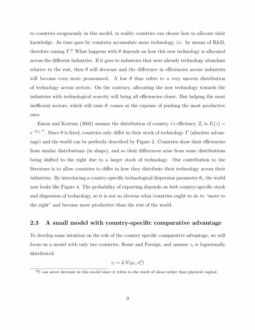
2.3 A small model with country-specific comparative advantage
To develop some intuition on the role of the country specific comparative advantage, we will
focus on a model with only two countries, Home and Foreign, and assume zi is lognormally
distributed:
zi ∼ LN(µi, σ2i )
9T can never decrease in this model since it refers to the stock of ideas rather than physical capital.
9
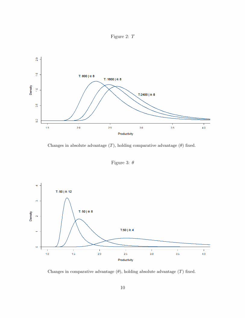
Figure 2: T
Changes in absolute advantage (T ), holding comparative advantage (θ) fixed.
Figure 3: θ
Changes in comparative advantage (θ), holding absolute advantage (T ) fixed.
10
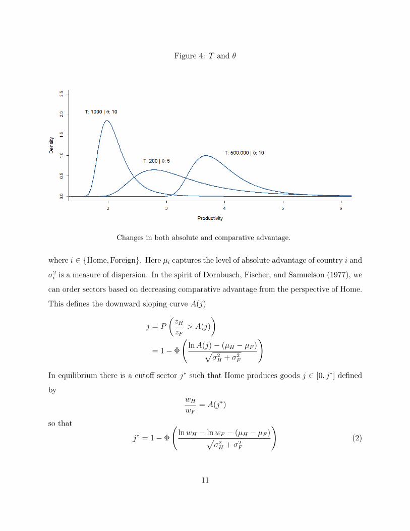
Figure 4: T and θ
Changes in both absolute and comparative advantage.
where i ∈ {Home,Foreign}. Here µi captures the level of absolute advantage of country i and
σ2i is a measure of dispersion. In the spirit of Dornbusch, Fischer, and Samuelson (1977), we
can order sectors based on decreasing comparative advantage from the perspective of Home.
This defines the downward sloping curve A(j)
j = P
(zHzF
> A(j)
)= 1− Φ
(lnA(j)− (µH − µF )√
σ2H + σ2
F
)
In equilibrium there is a cutoff sector j∗ such that Home produces goods j ∈ [0, j∗] defined
bywHwF
= A(j∗)
so that
j∗ = 1− Φ
(lnwH − lnwF − (µH − µF )√
σ2H + σ2
F
)(2)
11
What happens to the range of goods produced at Home when the dispersion parameter σ2H
increases? It depends on the equilibrium relative wage that appears in the numerator of
equation (2).
If we impose CES preferences then each country spends a fraction j∗ of their income in
goods produced at Home. Total spending in equilibrium has to equal total wages at Home
wHLH = j∗wHLH + j∗wFLF (3)
Starting from a symmetric case where LH = LF , it can be shown that (2) and (3) imply
∂j∗
∂σ2H
> 0 ⇐⇒ lnwH − lnwF > µH − µF ⇐⇒ µH < µF
so an increase in technological dispersion raises the range of goods produced at Home if and
only if Home is a technological follower (has less absolute advantage than Foreign). The
intuition behind this result is as follows. Home is on average more expensive than Foreign
and thus produces in equilibrium a narrower range of goods. As a result, an increase in
dispersion dampens the effect of absolute advantage and therefore increases the range of
goods produced at the country with less absolute advantage (technological follower). Notice
however that the effect depends on the initial values of dispersion by country σ2H and σ2
F .
2.4 Full model with country-specific comparative advantage
When θk is country-specific, the probability that country i provides a good at the lowest
price in country n is:
πni = P (pni(j) ≤ mink 6=i
pnk(j))
= P
(cidnizi(j)
≤ mink 6=i
ckdnkzk(j)
)=
∫ ∞0
ΠNk 6=ie
−Tk(ckdnkzicidni
)−θkθiTiz
−θi−1i e−Tiz
−θii dzi
=
∫ ∞0
e−∑Nk=1 Tk
(ckdnkzicidni
)−θkθiTiz
−θi−1i dzi (4)
12
In the appendix we show that the term inside the integral can be replaced by
N∑k=1
Tk
(ckdnkzicidni
)−θk=
N∑k=1
Tk
(ckdnkcidni
)−θkz−θii + ε
where the expectation of the approximation error E(ε) is second order. This approximation
treats the sum with heterogeneous θk as if it were a sum with a fixed θi, since differences in
the exponents will tend to cancel out.10 With this approximation, we can simplify expression
(4) to get
πni =Ti∑N
k=1 Tk
(ckdnkcidni
)−θk (5)
The term in the denominator is a measure of world competitiveness relative to country i. It
reflects how much cheaper (in terms of input and transport costs) the rest of the world is
relative to i. Intuitively, exporter i will be more successful if its technological level is higher
relative to world competitiveness. Since in this model πni is also the fraction that country n
spends in goods from i, equation (5) becomes:
Xni
Xn
=Ti∑N
k=1 Tk
(ckdnkcidni
)−θk (6)
The left hand side variable is normalized bilateral imports: i’s imports from n adjusted by
home purchases. We can think of (6) as the model’s gravity equation as it relates normalized
bilateral trade to the stock of technology, and relative input and transport costs (like wages
and geographic distance). Taking logs and expanding with respect to the θk parameters up
to a first order we get
lnXni
Xn
= lnTi − ln
(N∑k=1
Tk
(ckdnkcidni
)−θ)+
N∑k=1
αk ln
(ckdnkcidni
)(θk − θ) (7)
where αk is the relative standing of country k in world competitiveness
αk =Tk
(ckdnkcidni
)−θk∑N
j=1 Tj
(cjdnjcidni
)−θj10See appendix for an analysis of the accuracy of this approximation.
13
Equation (7) summarizes our model. Bilateral trade is related to the exporter’s technological
stock or absolute advantage (first term), a world competitiveness index (relative to i, second
term), and a comparative advantage term. Note that, if all countries have the same dispersion
parameter, θk = θ ∀k, the last term equals zero and our model simplifies to the benchmark
Eaton and Kortum (2002).11 This is an advantage of our setup, compared to others, as it
allows for easy comparison between the models.
The EK model, contained in the first two terms, provides a gravity equation to study
the effect of trade costs, represented by geography and technology, on the pattern of trade.
In particular, it predicts that exports from country i are larger when it has more absolute
advantage relative to world competitiveness. That is, country i will export more to country n
the more technology it accumulates and the higher the trade costs of the rest of the countries
(relative to i).12 The only role of the world technological dispersion parameter θ is in shaping
the elasticity of imports with respect to input costs and geographic barriers. Note that an
increase in the relative cost of any given country k will have a similar effect (henceforth,
the EK effect) on i as the model imposes a common dispersion θ for every country. In
other words, in the EK model, it doesn’t matter from the perspective of i’s exports to
n which competitor k experiences an increase in relative costs. Similarly, any increase in
world dispersion (θ) will benefit all exporters equally. But, as we already anticipated in the
introduction and will show in section 3, technological dispersion (measured with patenting
data) varies significantly across countries and these differences turn out to be important
determinants of bilateral trade.
The key feature of our model is, compared to the standard EK gravity, the additional
(third) term of equation (7). The comparative advantage term helps us to better understand
the effect of both a change in a country’s relative costs and a change in the dispersion
parameter on exports by introducing an effect that has been neglected so far in the literature:
that a country’s exports also depend on its relative world standing regarding costs and
11ln Xni
Xn= lnTi − ln
(∑Nk=1 Tk
(ckdnk
cidni
)−θ)12The trade costs have an exporter specific component (input costs) and a bilateral pair component (i.e.
geographic distance).
14
technology. So any changes in a competitor’s k input costs or technological dispersion (i.e.
they become more technologically specialized or diversified) will affect i’s exports to n.
With regard to relative costs, the baseline EK effect still holds and is captured by our world
competitiveness (second) term. An increase in k’s costs relative to i will benefit i’s exports
to n. However, there is an additional effect coming from the comparative advantage (third)
term so the overall effect can be augmented or dampened depending on the magnitude of
productivity dispersion parameter θk. The effect will be larger when θk is large, that is,
when productivity dispersion is smaller. Since country k’s force of comparative advantage is
weaker any given change in k’s costs has a larger effect on i’s exports.
Our model captures, through the comparative advantage term, how the country-specific
productivity dispersion co-varies with relative costs. We can see from equation (7) that the
effect of an increase in θk depends on the sign of the log of relative costs. If country k
is relatively less competitive (has higher costs relative to i), then the log term is positive
and an increase in θk increases exports from i to n. Intuitively, a larger θk dampens the
force of comparative advantage and increases the effect of a difference in relative costs.
This effect was already present in the two country model of Section 2.3. A reduction in
productivity dispersion increases exports of the country that is relatively less expensive. In
the multicountry case, we also observe that this effect is larger when αk is big: an increase
in θk favors country i’s exports, especially if country k is highly competitive relative to the
world’s average competitiveness index.
When is country k relatively more expensive than country i? The answer was already
provided in the two country model of Section 2.3, which suggested that in a two country world
with log-normal productivity, the country with a higher absolute advantage was relatively
less expensive. If we assume labor is the only input in production, the equilibrium in the
multicountry model is given by
wiLi =N∑n=1
πniwnLn
We can solve the model in closed form if we assume no trade barriers, so that dni = 1 for all
15
country pairs, and a common dispersion parameter θ for all countries. In that case we get:
wn/T1/θn
wi/T1/θi
=
(T
1/θn /Ln
T1/θi /Li
)− 11+θ
so that if country n has higher absolute advantage measured by T1/θn then it will be more
competitive in terms of productivity adjusted labor costs.
3 Data Description
We build a unique panel dataset containing measures of the stock of technology T , the
productivity dispersion θ, bilateral trade, input costs, trade costs, and other bilateral char-
acteristics (like shared language or border) for 84 developed and developing countries, from
1980 to 2000.13 We follow Eaton and Kortum (2010) in understanding technology as the
outcome of a process that starts with an idea, and therefore use patent data to measure the
technological stock and dispersion. These two are then used to construct the absolute and
comparative advantage variables T and θ in a theory-consistent way, which constitutes one of
the main contributions of this paper. For the rest of the variables we follow the literature in
choosing widely used measures and databases. To measure trade we use UN COMTRADE
bilateral imports. Data on GDP per capita by country and year is from the World Bank’s
World Development Indicators (WDI). Our measures of trade costs (geographic distance,
common language, border, common currency, common colonizer, etc.) by bilateral pair are
from CEPII gravdata dataset. Finally, we use data on wages by country and year from the
International Labour Organization (ILO). Below we describe the sources of the technological
data and the construction of the key variables.
3.1 Patent Data
Patent grants at the USPTO are our indicator of technological capabilities of countries.
Data on patenting activity covering the period 1975-2000 was obtained from the “Patent
13A list of all countries can be found in the Data Appendix.
16
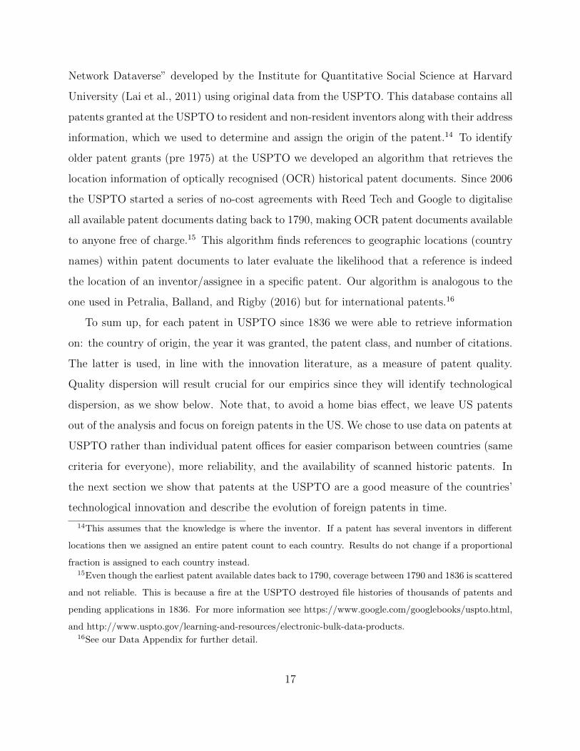
Network Dataverse” developed by the Institute for Quantitative Social Science at Harvard
University (Lai et al., 2011) using original data from the USPTO. This database contains all
patents granted at the USPTO to resident and non-resident inventors along with their address
information, which we used to determine and assign the origin of the patent.14 To identify
older patent grants (pre 1975) at the USPTO we developed an algorithm that retrieves the
location information of optically recognised (OCR) historical patent documents. Since 2006
the USPTO started a series of no-cost agreements with Reed Tech and Google to digitalise
all available patent documents dating back to 1790, making OCR patent documents available
to anyone free of charge.15 This algorithm finds references to geographic locations (country
names) within patent documents to later evaluate the likelihood that a reference is indeed
the location of an inventor/assignee in a specific patent. Our algorithm is analogous to the
one used in Petralia, Balland, and Rigby (2016) but for international patents.16
To sum up, for each patent in USPTO since 1836 we were able to retrieve information
on: the country of origin, the year it was granted, the patent class, and number of citations.
The latter is used, in line with the innovation literature, as a measure of patent quality.
Quality dispersion will result crucial for our empirics since they will identify technological
dispersion, as we show below. Note that, to avoid a home bias effect, we leave US patents
out of the analysis and focus on foreign patents in the US. We chose to use data on patents at
USPTO rather than individual patent offices for easier comparison between countries (same
criteria for everyone), more reliability, and the availability of scanned historic patents. In
the next section we show that patents at the USPTO are a good measure of the countries’
technological innovation and describe the evolution of foreign patents in time.
14This assumes that the knowledge is where the inventor. If a patent has several inventors in different
locations then we assigned an entire patent count to each country. Results do not change if a proportional
fraction is assigned to each country instead.15Even though the earliest patent available dates back to 1790, coverage between 1790 and 1836 is scattered
and not reliable. This is because a fire at the USPTO destroyed file histories of thousands of patents and
pending applications in 1836. For more information see https://www.google.com/googlebooks/uspto.html,
and http://www.uspto.gov/learning-and-resources/electronic-bulk-data-products.16See our Data Appendix for further detail.
17
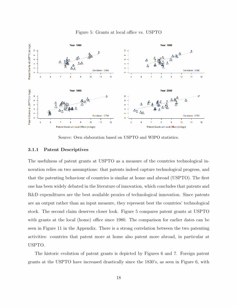
Figure 5: Grants at local office vs. USPTO
Source: Own elaboration based on USPTO and WIPO statistics.
3.1.1 Patent Descriptives
The usefulness of patent grants at USPTO as a measure of the countries technological in-
novation relies on two assumptions: that patents indeed capture technological progress, and
that the patenting behaviour of countries is similar at home and abroad (USPTO). The first
one has been widely debated in the literature of innovation, which concludes that patents and
R&D expenditures are the best available proxies of technological innovation. Since patents
are an output rather than an input measure, they represent best the countries’ technological
stock. The second claim deserves closer look. Figure 5 compares patent grants at USPTO
with grants at the local (home) office since 1980. The comparison for earlier dates can be
seen in Figure 11 in the Appendix. There is a strong correlation between the two patenting
activities: countries that patent more at home also patent more abroad, in particular at
USPTO.
The historic evolution of patent grants is depicted by Figures 6 and 7. Foreign patent
grants at the USPTO have increased drastically since the 1830’s, as seen in Figure 6, with
18
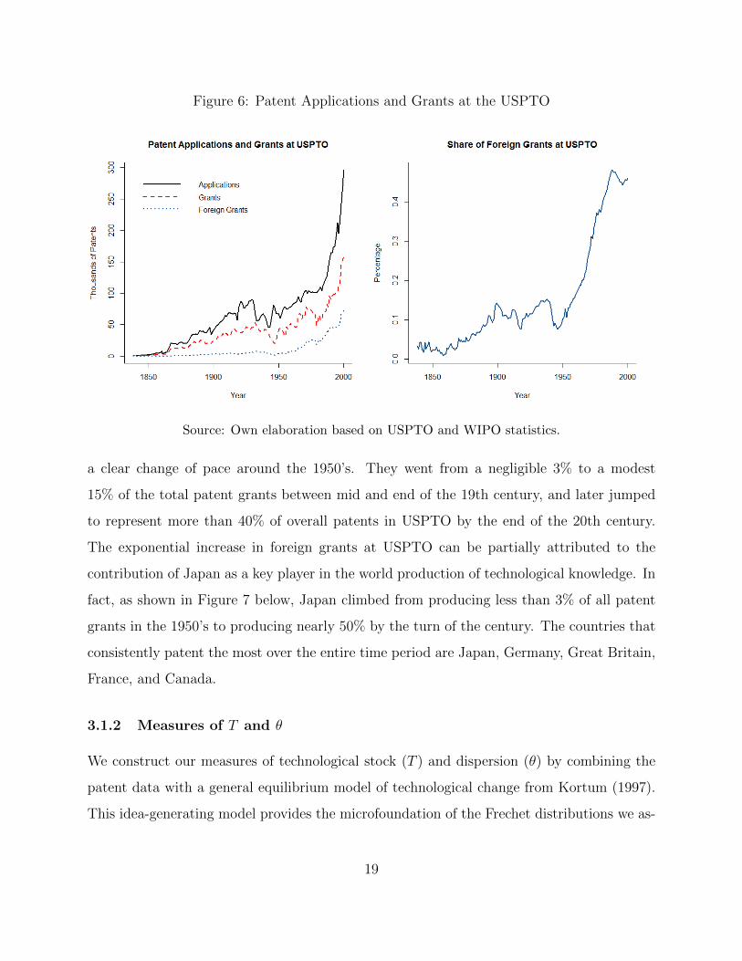
Figure 6: Patent Applications and Grants at the USPTO
Source: Own elaboration based on USPTO and WIPO statistics.
a clear change of pace around the 1950’s. They went from a negligible 3% to a modest
15% of the total patent grants between mid and end of the 19th century, and later jumped
to represent more than 40% of overall patents in USPTO by the end of the 20th century.
The exponential increase in foreign grants at USPTO can be partially attributed to the
contribution of Japan as a key player in the world production of technological knowledge. In
fact, as shown in Figure 7 below, Japan climbed from producing less than 3% of all patent
grants in the 1950’s to producing nearly 50% by the turn of the century. The countries that
consistently patent the most over the entire time period are Japan, Germany, Great Britain,
France, and Canada.
3.1.2 Measures of T and θ
We construct our measures of technological stock (T ) and dispersion (θ) by combining the
patent data with a general equilibrium model of technological change from Kortum (1997).
This idea-generating model provides the microfoundation of the Frechet distributions we as-
19
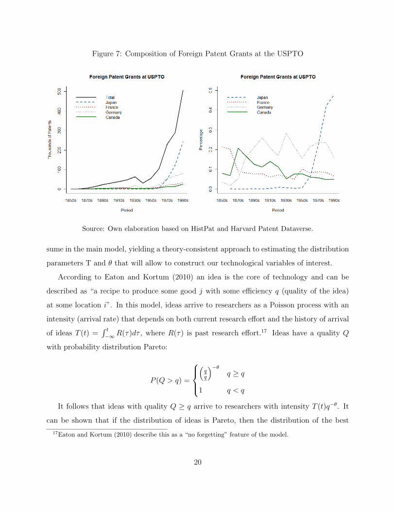
Figure 7: Composition of Foreign Patent Grants at the USPTO
Source: Own elaboration based on HistPat and Harvard Patent Dataverse.
sume in the main model, yielding a theory-consistent approach to estimating the distribution
parameters T and θ that will allow to construct our technological variables of interest.
According to Eaton and Kortum (2010) an idea is the core of technology and can be
described as “a recipe to produce some good j with some efficiency q (quality of the idea)
at some location i”. In this model, ideas arrive to researchers as a Poisson process with an
intensity (arrival rate) that depends on both current research effort and the history of arrival
of ideas T (t) =∫ t−∞R(τ)dτ , where R(τ) is past research effort.17 Ideas have a quality Q
with probability distribution Pareto:
P (Q > q) =
)−θq ≥ q
1 q < q
It follows that ideas with quality Q ≥ q arrive to researchers with intensity T (t)q−θ. It
can be shown that if the distribution of ideas is Pareto, then the distribution of the best
17Eaton and Kortum (2010) describe this as a “no forgetting” feature of the model.
20
ideas is Frechet with parameters T and θ.
The probability that yi ideas (patents) with quality qi arrive at a given year is
P (Y = y) =∏i
e−T (t)q−θi
(T (t)q−θi )yi
yi!
We obtain values for idea qualities based on citations and proxy T with the stock of patents
at time t.
T (t) =t∑
k=1836
Patentsk
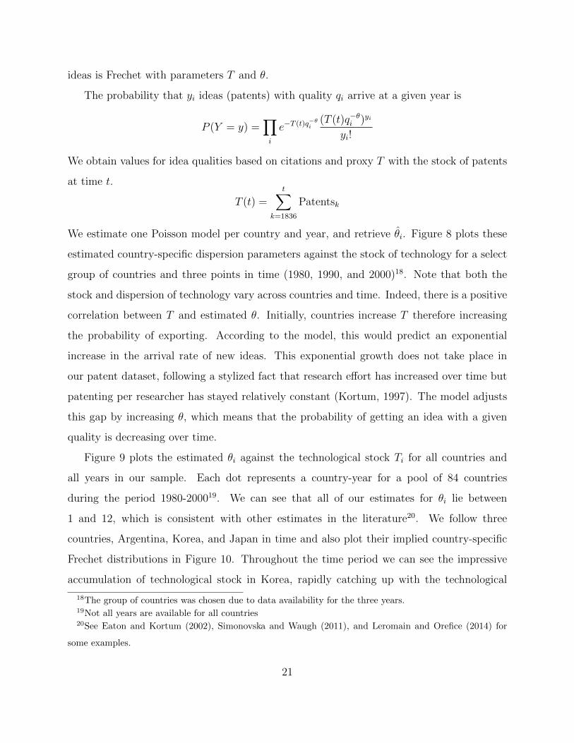
We estimate one Poisson model per country and year, and retrieve θ̂i. Figure 8 plots these
estimated country-specific dispersion parameters against the stock of technology for a select
group of countries and three points in time (1980, 1990, and 2000)18. Note that both the
stock and dispersion of technology vary across countries and time. Indeed, there is a positive
correlation between T and estimated θ. Initially, countries increase T therefore increasing
the probability of exporting. According to the model, this would predict an exponential
increase in the arrival rate of new ideas. This exponential growth does not take place in
our patent dataset, following a stylized fact that research effort has increased over time but
patenting per researcher has stayed relatively constant (Kortum, 1997). The model adjusts
this gap by increasing θ, which means that the probability of getting an idea with a given
quality is decreasing over time.
Figure 9 plots the estimated θi against the technological stock Ti for all countries and
all years in our sample. Each dot represents a country-year for a pool of 84 countries
during the period 1980-200019. We can see that all of our estimates for θi lie between
1 and 12, which is consistent with other estimates in the literature20. We follow three
countries, Argentina, Korea, and Japan in time and also plot their implied country-specific
Frechet distributions in Figure 10. Throughout the time period we can see the impressive
accumulation of technological stock in Korea, rapidly catching up with the technological
18The group of countries was chosen due to data availability for the three years.19Not all years are available for all countries20See Eaton and Kortum (2002), Simonovska and Waugh (2011), and Leromain and Orefice (2014) for
some examples.
21
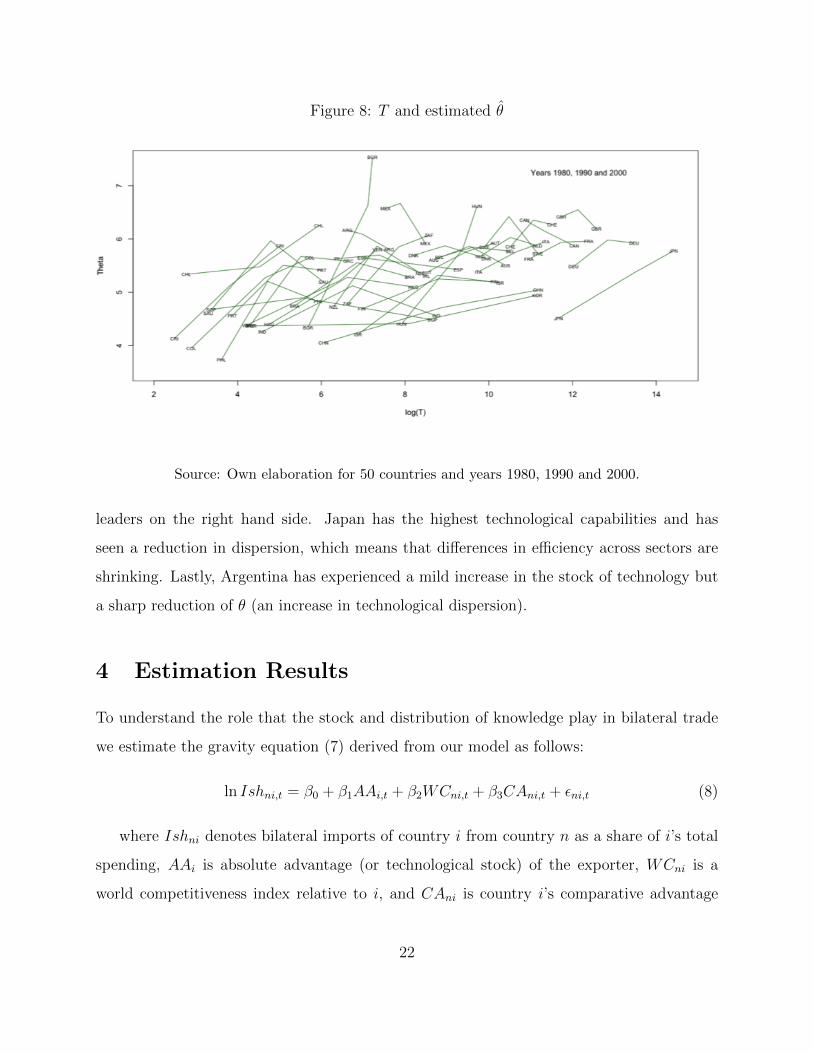
Figure 8: T and estimated θ̂
Source: Own elaboration for 50 countries and years 1980, 1990 and 2000.
leaders on the right hand side. Japan has the highest technological capabilities and has
seen a reduction in dispersion, which means that differences in efficiency across sectors are
shrinking. Lastly, Argentina has experienced a mild increase in the stock of technology but
a sharp reduction of θ (an increase in technological dispersion).
4 Estimation Results
To understand the role that the stock and distribution of knowledge play in bilateral trade
we estimate the gravity equation (7) derived from our model as follows:
ln Ishni,t = β0 + β1AAi,t + β2WCni,t + β3CAni,t + εni,t (8)
where Ishni denotes bilateral imports of country i from country n as a share of i’s total
spending, AAi is absolute advantage (or technological stock) of the exporter, WCni is a
world competitiveness index relative to i, and CAni is country i’s comparative advantage
22
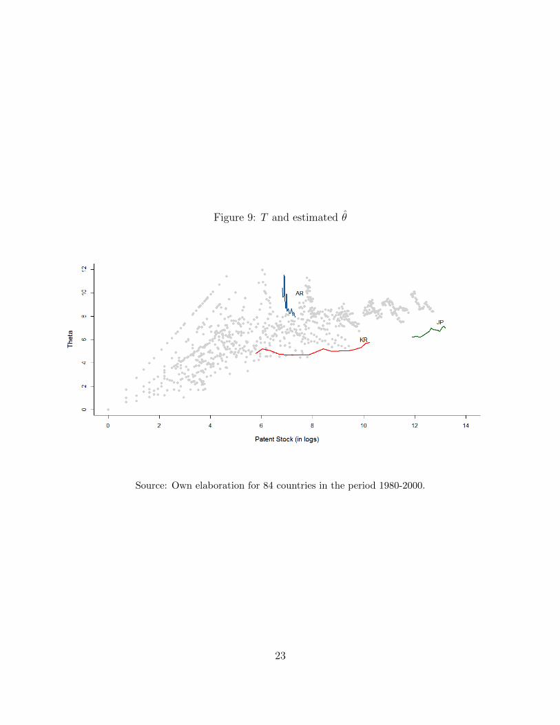
Figure 9: T and estimated θ̂
Source: Own elaboration for 84 countries in the period 1980-2000.
23
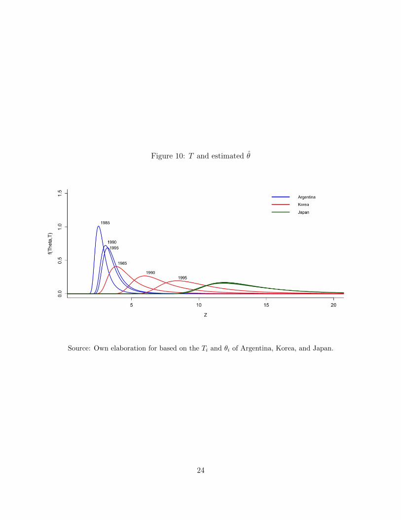
Figure 10: T and estimated θ̂
Source: Own elaboration for based on the Ti and θi of Argentina, Korea, and Japan.
24
when selling to n. Finally, t represents time (in years). All variables are as defined in
equation (7) and have been calculated using the data described above.
Our model is a generalized version of Eaton and Kortum (2002), represented by the terms
AAi,t and WCni,t. One advantage of this setup is that it allows for a straightforward compar-
ison between the models, so we can assess the relevance of the distribution of knowledge that
enters through our term CAni,t. Moreover, this term represents our main contribution as
it introduces the two main aspects of classical Ricardian theory to the multi-country setup:
that technological dispersion is country-specific, and that it matters for bilateral exports. In
our formulation, the latter takes the form of an augmenting (or dampening) trade effect to
decreasing the exporter’s relative costs. Our theory predicts that β2 is negative and β1 and
β3 are positive. Bilateral exports from i to n decrease with i’s trading costs (relative to the
rest of the world’s) and increase with i’s technological stock and relative force of compar-
ative advantage. In particular, as we discussed earlier, country i will benefit more from a
decrease in a competitor’s force of comparative advantage (reduced technological dispersion)
the cheaper i is relative to its competitors.
Table 1 reports the results of estimating equation (8) for over 2200 country pairs in 18
years, comparing the baseline EK model (first two terms) to our generalized (full) model
across different specifications. To keep our econometric model closer to the empirical litera-
ture, we include the usual controls. Note that the economic interpretation of the comparative
advantage coefficient is not very straightforward. The CA term represents how relative costs
covary with technological dispersion, and thus we interpret its coefficient as the elasticity of
exports with respect to the cost-dispersion covariance.
The results in columns (1) and (2) of Table 1 reveal that, after accounting for exporter
fixed effects, all absolute advantage, world competitiveness, and comparative advantage
terms matter for bilateral trade. All coefficients have the expected sign and are highly
significant, which supports our model and suggests that the standard EK model was omit-
ting a relevant determinant of exports. Columns (3) and (4) of Table 1 report the results of
estimating both models after adding time fixed effects. The coefficient on absolute advantage
25
drops while the others remain virtually unchanged. Finally, columns (5) and (6) of Table
1 report the results of estimating both models after introducing the typical bilateral trade
costs determinants from the gravity literature. These allow to control for common shared
characteristics constant in time, such as common language, shared border, colonial ties and
shared past. The full table of results (including these gravity coefficients) can be seen in
the Appendix. The results are very similar to the previous specification and all the gravity
variables are significant and have the expected signs. This is our preferred specification.
Overall, our results suggest that, in line with the existing Ricardian literature, an increase
in the overall stock of technology or a decrease in relative costs of the exporter i increases
its exports to n. In addition, we find that the comparative advantage term matters, sup-
porting our augmented (full) model. This evidence suggests that changes in country-specific
technological dispersion are important determinants of bilateral trade.
In Table 2 we show that our main finding is robust to alternative specifications and
measures of costs. So far we have followed Eaton and Kortum (2002) in using wages to
measure costs. One concern with this measure is that wages only capture the labor com-
ponent of production costs, so now we turn to using the wholesale price index (WPI) as an
alternative measure. Columns (1) and (2) of Table 2 report the results of estimating our
preferred specification when using wages and WPI, respectively. All coefficients are similar
in magnitude, have the expected signs, and are significant. In columns (3) and (4) of Table
2 show the estimation results after adding exporter-time fixed effects with both measures
of costs. The comparative advantage term gets absorbed by the fixed effects, but both the
world competitiveness term and the comparative advantage term are statistically significant
and have the right signs. Finally, we drop the bilateral controls and exporter-time effects
and replace them with bilateral pair fixed effects. Columns (5) and (6) report the results
of estimating equation (8) for both measures of costs. As expected, the significance of the
comparative advantage effect is diminished, but all results still hold when using wages as the
cost measure.
26
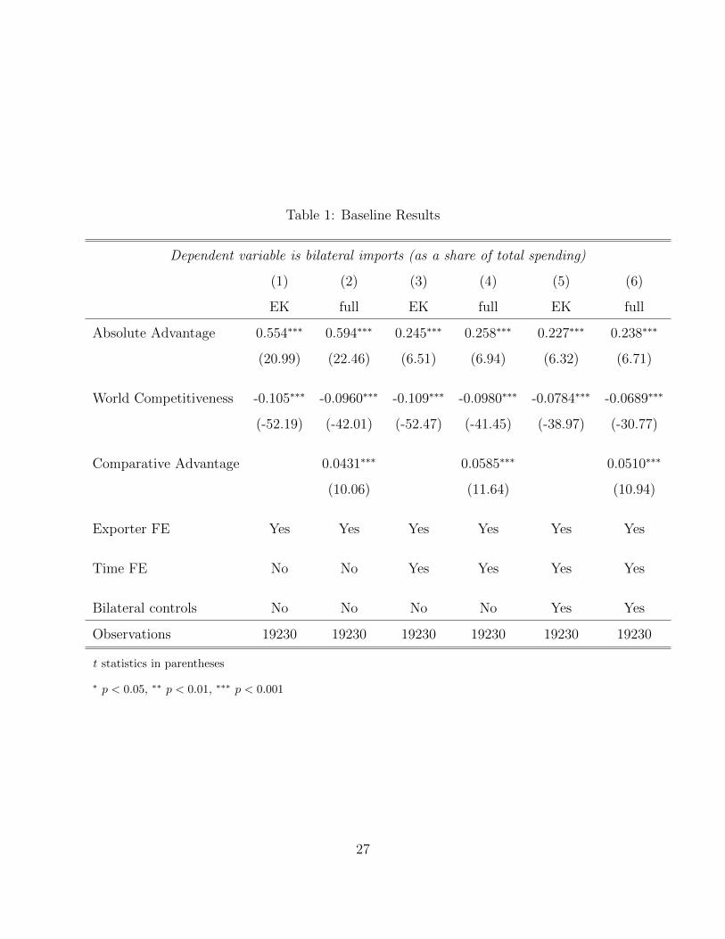
Table 1: Baseline Results
Dependent variable is bilateral imports (as a share of total spending)
(1) (2) (3) (4) (5) (6)
EK full EK full EK full
Absolute Advantage 0.554∗∗∗ 0.594∗∗∗ 0.245∗∗∗ 0.258∗∗∗ 0.227∗∗∗ 0.238∗∗∗
(20.99) (22.46) (6.51) (6.94) (6.32) (6.71)
World Competitiveness -0.105∗∗∗ -0.0960∗∗∗ -0.109∗∗∗ -0.0980∗∗∗ -0.0784∗∗∗ -0.0689∗∗∗
(-52.19) (-42.01) (-52.47) (-41.45) (-38.97) (-30.77)
Comparative Advantage 0.0431∗∗∗ 0.0585∗∗∗ 0.0510∗∗∗
(10.06) (11.64) (10.94)
Exporter FE Yes Yes Yes Yes Yes Yes
Time FE No No Yes Yes Yes Yes
Bilateral controls No No No No Yes Yes
Observations 19230 19230 19230 19230 19230 19230
t statistics in parentheses
∗ p < 0.05, ∗∗ p < 0.01, ∗∗∗ p < 0.001
27
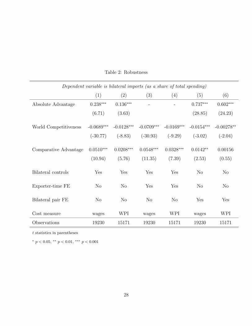
Table 2: Robustness
Dependent variable is bilateral imports (as a share of total spending)
(1) (2) (3) (4) (5) (6)
Absolute Advantage 0.238∗∗∗ 0.136∗∗∗ - - 0.737∗∗∗ 0.602∗∗∗
(6.71) (3.63) (28.85) (24.23)
World Competitiveness -0.0689∗∗∗ -0.0128∗∗∗ -0.0709∗∗∗ -0.0169∗∗∗ -0.0154∗∗∗ -0.00278∗∗
(-30.77) (-8.83) (-30.93) (-9.29) (-3.02) (-2.04)
Comparative Advantage 0.0510∗∗∗ 0.0208∗∗∗ 0.0548∗∗∗ 0.0328∗∗∗ 0.0142∗∗ 0.00156
(10.94) (5.76) (11.35) (7.39) (2.53) (0.55)
Bilateral controls Yes Yes Yes Yes No No
Exporter-time FE No No Yes Yes No No
Bilateral pair FE No No No No Yes Yes
Cost measure wages WPI wages WPI wages WPI
Observations 19230 15171 19230 15171 19230 15171
t statistics in parentheses
∗ p < 0.05, ∗∗ p < 0.01, ∗∗∗ p < 0.001
28
5 Concluding Remarks
This paper documents that there is a high range of country-level technological dispersion as
measured by patent data. In addition, this measure appears to be highly correlated with
international trade flows. The literature, however, has managed to explain only the relation-
ship between the technological stock and trade flows, thus ignoring the role of dispersion.
Building on Eaton and Kortum (2002), we have developed a Ricardian model that takes
into account the role of absolute advantage and technological dispersion, both of which
are country-specific. We have shown that one is not independent of the other: the theory
predicts that their interaction is also important for explaining bilateral trade. In particular,
the effect of increasing technological dispersion depends on the relative world standing of a
given country, as measured by its technological stock. In the model, technological dispersion
governs the advantage of having lower input costs. A lower dispersion benefits countries
with lower input costs since their exports are determined by these and not technological
differences. The effect is reversed for the countries with which they are competing. This
observation results in the main prediction of the model: a given country’s exports increase
when competitors with low costs have high dispersion of technology and competitors with
high costs have low dispersion.
To test our theory we rely on measures of technological variables that allow to test the
predictions of the model. These should represent absolute and comparative advantage, be
originated from outside of the model and consistent with the theory. To this end, we create
a novel dataset of historical patents (the longest to date) using patent grants at the USPTO.
We use the dataset to construct measures of the stock and dispersion of technology that are
consistent with the theoretical model. We combine the patent data with data on exports,
patents, input costs, income, expenditures, and bilateral pair characteristics for 84 developed
and developing exporters in the period 1983-2000.
Our empirical results confirm our theoretical predictions: both the stock and the disper-
sion of technology are important determinants of exports, and countries are affected by their
relative world standing in terms of costs and technological stock and dispersion. Future work
29
should focus in using this model to explain the diversification patterns in export behavior.
30
6 Appendix
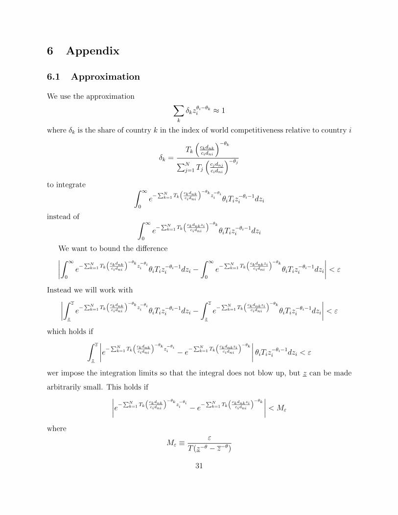
6.1 Approximation
We use the approximation ∑k
δkzθi−θki ≈ 1
where δk is the share of country k in the index of world competitiveness relative to country i
δk =Tk
(ckdnkcidni
)−θk∑N
j=1 Tj
(cjdnjcidni
)−θjto integrate ∫ ∞
0
e−∑Nk=1 Tk
(ckdnkcidni
)−θkz−θii θiTiz
−θi−1i dzi
instead of ∫ ∞0
e−∑Nk=1 Tk
(ckdnkzicidni
)−θkθiTiz
−θi−1i dzi
We want to bound the difference∣∣∣∣∫ ∞0
e−∑Nk=1 Tk
(ckdnkcidni
)−θkz−θii θiTiz
−θi−1i dzi −
∫ ∞0
e−∑Nk=1 Tk
(ckdnkzicidni
)−θkθiTiz
−θi−1i dzi
∣∣∣∣ < ε
Instead we will work with∣∣∣∣∫ z
z
e−∑Nk=1 Tk
(ckdnkcidni
)−θkz−θii θiTiz
−θi−1i dzi −
∫ z
z
e−∑Nk=1 Tk
(ckdnkzicidni
)−θkθiTiz
−θi−1i dzi
∣∣∣∣ < ε
which holds if∫ z
z
∣∣∣∣e−∑Nk=1 Tk
(ckdnkcidni
)−θkz−θii − e−
∑Nk=1 Tk
(ckdnkzicidni
)−θk ∣∣∣∣ θiTiz−θi−1i dzi < ε
wer impose the integration limits so that the integral does not blow up, but z can be made
arbitrarily small. This holds if∣∣∣∣e−∑Nk=1 Tk
(ckdnkcidni
)−θkz−θii − e−
∑Nk=1 Tk
(ckdnkzicidni
)−θk ∣∣∣∣ < Mε
where
Mε ≡ε
T (z−θ − z−θ)
31
which holds if ∣∣∣∣∣∣e−∑Nk=1 Tk
(ckdnkcidni
)−θkz−θii − e−
∑Nk=1 Tk
(ckdnkzicidni
)−θke−∑Nk=1 Tk
(ckdnkcidni
)−θkz−θii
∣∣∣∣∣∣ < Mε
or ∣∣∣∣1− e∑Nk=1 Tk
(ckdnkcidni
)−θkz−θii −
∑Nk=1 Tk
(ckdnkzicidni
)−θk ∣∣∣∣ < Mε
This holds if ∣∣∣∣∣1− e−∣∣∣∣∑N
k=1 Tk
(ckdnkcidni
)−θkz−θii −
∑Nk=1 Tk
(ckdnkzicidni
)−θk ∣∣∣∣∣∣∣∣∣ < Mε
or alternatively
− ln (1 +Mε) <
∣∣∣∣∣N∑k=1
Tk
(ckdnkcidni
)−θkz−θii −
N∑k=1
Tk
(ckdnkzicidni
)−θk∣∣∣∣∣ < − ln (1−Mε)
And a first order Taylor expansion gives
− ln (1 +Mε)
ln z/zθ<
∣∣∣∣∣N∑k=1
Tk
(ckdnkcidni
)−θk|θk − θi|
∣∣∣∣∣ < − ln (1−Mε)
ln z/zθ
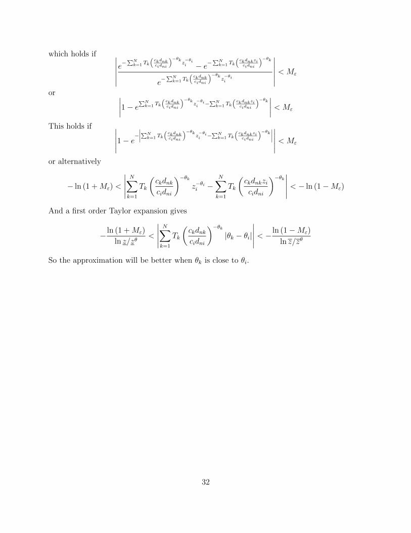
So the approximation will be better when θk is close to θi.
32
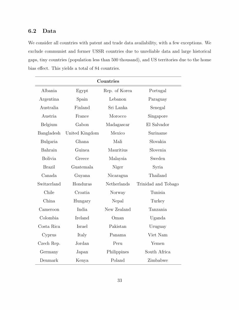
6.2 Data
We consider all countries with patent and trade data availability, with a few exceptions. We
exclude communist and former USSR countries due to unreliable data and large historical
gaps, tiny countries (population less than 500 thousand), and US territories due to the home
bias effect. This yields a total of 84 countries.
Countries
Albania Egypt Rep. of Korea Portugal
Argentina Spain Lebanon Paraguay
Australia Finland Sri Lanka Senegal
Austria France Morocco Singapore
Belgium Gabon Madagascar El Salvador
Bangladesh United Kingdom Mexico Suriname
Bulgaria Ghana Mali Slovakia
Bahrain Guinea Mauritius Slovenia
Bolivia Greece Malaysia Sweden
Brazil Guatemala Niger Syria
Canada Guyana Nicaragua Thailand
Switzerland Honduras Netherlands Trinidad and Tobago
Chile Croatia Norway Tunisia
China Hungary Nepal Turkey
Cameroon India New Zealand Tanzania
Colombia Ireland Oman Uganda
Costa Rica Israel Pakistan Uruguay
Cyprus Italy Panama Viet Nam
Czech Rep. Jordan Peru Yemen
Germany Japan Philippines South Africa
Denmark Kenya Poland Zimbabwe
33
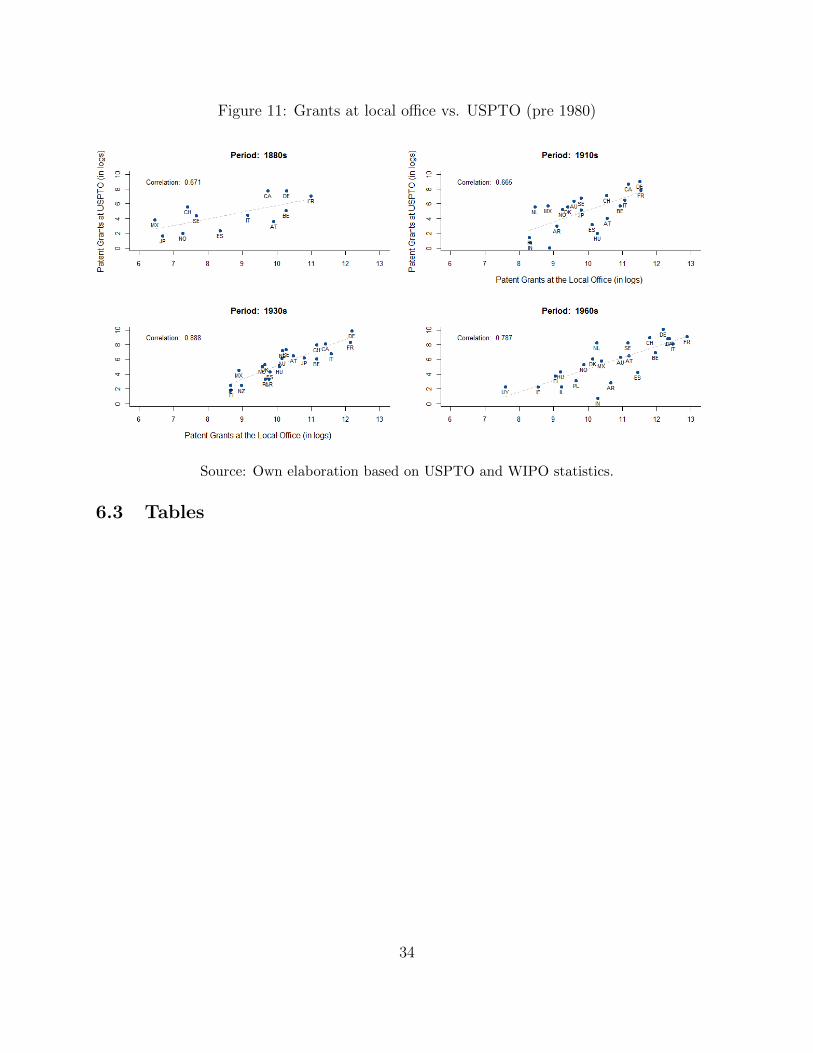
Figure 11: Grants at local office vs. USPTO (pre 1980)
Source: Own elaboration based on USPTO and WIPO statistics.
6.3 Tables
34
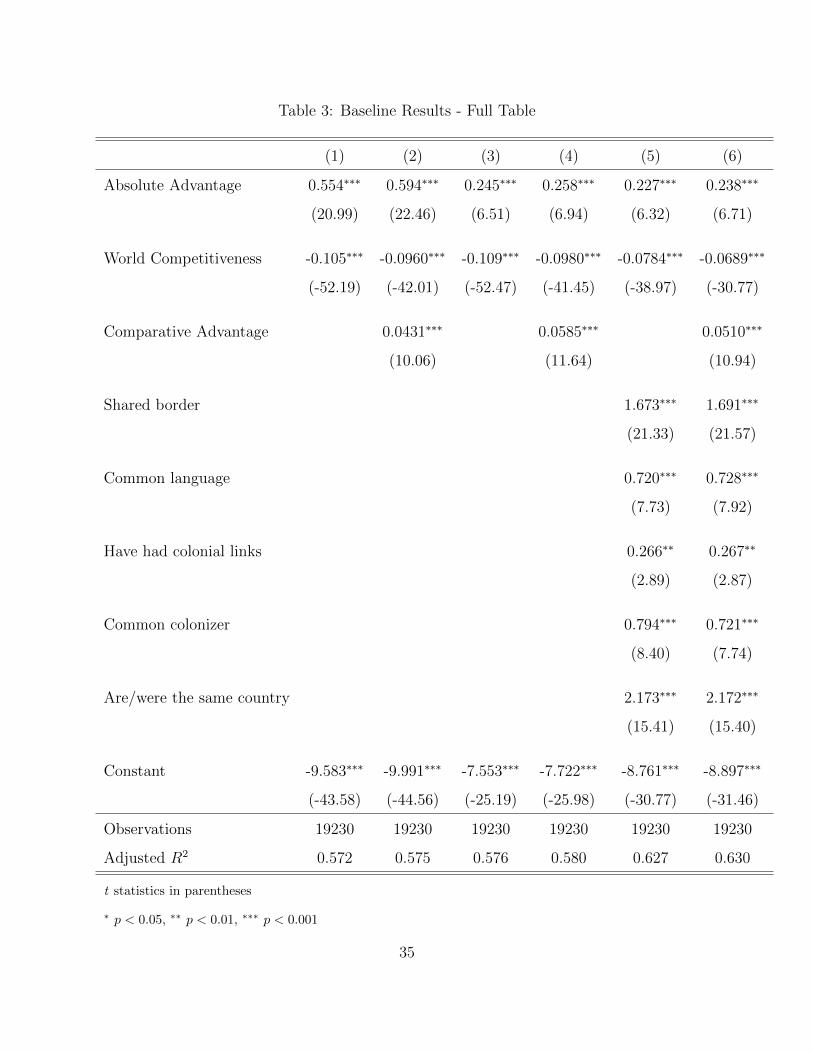
Table 3: Baseline Results - Full Table
(1) (2) (3) (4) (5) (6)
Absolute Advantage 0.554∗∗∗ 0.594∗∗∗ 0.245∗∗∗ 0.258∗∗∗ 0.227∗∗∗ 0.238∗∗∗
(20.99) (22.46) (6.51) (6.94) (6.32) (6.71)
World Competitiveness -0.105∗∗∗ -0.0960∗∗∗ -0.109∗∗∗ -0.0980∗∗∗ -0.0784∗∗∗ -0.0689∗∗∗
(-52.19) (-42.01) (-52.47) (-41.45) (-38.97) (-30.77)
Comparative Advantage 0.0431∗∗∗ 0.0585∗∗∗ 0.0510∗∗∗
(10.06) (11.64) (10.94)
Shared border 1.673∗∗∗ 1.691∗∗∗
(21.33) (21.57)
Common language 0.720∗∗∗ 0.728∗∗∗
(7.73) (7.92)
Have had colonial links 0.266∗∗ 0.267∗∗
(2.89) (2.87)
Common colonizer 0.794∗∗∗ 0.721∗∗∗
(8.40) (7.74)
Are/were the same country 2.173∗∗∗ 2.172∗∗∗
(15.41) (15.40)
Constant -9.583∗∗∗ -9.991∗∗∗ -7.553∗∗∗ -7.722∗∗∗ -8.761∗∗∗ -8.897∗∗∗
(-43.58) (-44.56) (-25.19) (-25.98) (-30.77) (-31.46)
Observations 19230 19230 19230 19230 19230 19230
Adjusted R2 0.572 0.575 0.576 0.580 0.627 0.630
t statistics in parentheses
∗ p < 0.05, ∗∗ p < 0.01, ∗∗∗ p < 0.001
35
References
Bloom, N., M. Draca, and J. Van Reenen (2015): “Trade induced technical change?
The impact of Chinese imports on innovation, IT and productivity,” The Review of Eco-
nomic Studies, p. rdv039.
Bolatto, S. (2013): “Trade across Countries and Manufacturing Sectors with Hetero-
geneous Trade Elasticities,” Centro Studi Luca d’Agliano Development Studies Working
Paper, (360).
Bustos, P. (2011): “Trade liberalization, exports, and technology upgrading: Evidence
on the impact of MERCOSUR on Argentinian firms,” The American economic review,
101(1), 304–340.
Caliendo, L., and F. Parro (2014): “Estimates of the Trade and Welfare Effects of
NAFTA,” The Review of Economic Studies, pp. 229–242.
Chor, D. (2010): “Unpacking sources of comparative advantage: A quantitative approach,”
Journal of International Economics, 82(2), 152–167.
Costinot, A., D. Donaldson, and I. Komunjer (2012): “What goods do countries
trade? A quantitative exploration of Ricardo’s ideas,” The Review of Economic Studies,
79(2), 581–608.
Donaldson, D. (2010): “Railroads of the Raj: Estimating the impact of transportation
infrastructure,” Discussion paper, National Bureau of Economic Research.
Dornbusch, R., S. Fischer, and P. A. Samuelson (1977): “Comparative advantage,
trade, and payments in a Ricardian model with a continuum of goods,” The American
Economic Review, pp. 823–839.
Eaton, J., and S. Kortum (2002): “Technology, geography, and trade,” Econometrica,
pp. 1741–1779.
(2010): “Technology in the Global Economy: A Framework for Quantitative Anal-
36
ysis,” Unpublished manuscript.
Kerr, W. R. (2013): “Heterogeneous technology diffusion and Ricardian trade patterns,”
Discussion paper, National Bureau of Economic Research.
Kortum, S. S. (1997): “Research, patenting, and technological change,” Econometrica:
Journal of the Econometric Society, pp. 1389–1419.
Leromain, E., and G. Orefice (2014): “New revealed comparative advantage index:
dataset and empirical distribution,” International Economics, 139, 48–70.
Levchenko, A. A., and J. Zhang (2016): “The evolution of comparative advantage:
Measurement and welfare implications,” Journal of Monetary Economics, 78, 96–111.
Lileeva, A., and D. Trefler (2010): “Improved access to foreign markets raises plant-
level productivity...for some plants,” The Quarterly Journal of Economics, 125(3), 1051–
1099.
OECD (2015): “Innovation Strategy 2015,” OECD Publishing.
Petralia, S., P.-A. Balland, and D. L. Rigby (2016): “Unveiling the geography of
historical patents in the United States from 1836 to 1975,” Scientific data, 3.
Posner, M. V. (1961): “International trade and technical change,” Oxford economic papers,
pp. 323–341.
Shikher, S. (2011): “Capital, technology, and specialization in the neoclassical model,”
Journal of international Economics, 83(2), 229–242.
Simonovska, I., and M. Waugh (2011): “The elasticity of trade: Evidence and esti-
mates,” Discussion paper, CESifo Working Paper Series.
Steinwender, C. (2015): “The roles of import competition and export opportunities for
technical change,” Centre for Economic Performance (CEP) Discussion Paper 1334.
Vernon, R. (1966): “International investment and international trade in the product cy-
cle,” The Quarterly Journal of Economics, pp. 190–207.
37