Takustr. 714195 Berlin

GermanyZuse Institute Berlin

KONSTANTIN FACKELDEY1, PETER KOLTAI2,PETER NEVIR AND HENNING RUST3

AXEL SCHILD4, MARCUS WEBER5

1Institut fur Mathematik, TU Berlin, Strasse des 17. Juni 136, 10623 Berlin

2Institut fur Mathematik, FU Berlin, Arnimallee 6, 14195 Berlin

3Institut fur Meteorologie, FU Berlin, Carl-Heinrich-Becker-Weg 6-10, 12165 Berlin

4Laboratorium fur Physikalische Chemie, ETH Zurich, Vladimir-Prelog-Weg 2, 8093 Zurich,

5Zuse Institute Berlin, Takustrasse 7, 14195 Berlin

From Metastable to CoherentSets – time-discretization

schemes

ZIB Report 17-74 (December 2017)

Zuse Institute BerlinTakustr. 714195 BerlinGermany

Telephone: +49 30-84185-0Telefax: +49 30-84185-125

E-mail: bibliothek@zib.deURL: http://www.zib.de

ZIB-Report (Print) ISSN 1438-0064ZIB-Report (Internet) ISSN 2192-7782

From Metastable to Coherent Sets – time-discretization schemes

Konstantin FackeldeyInstitut für Mathematik, TU Berlin, Straße des 17. Juni 136,

10623 Berlin, Email: fackeldey@math.tu-berlin.de

Péter KoltaiInstitut für Mathematik, FU Berlin, Arnimallee 6, 14195 Berlin, Email: peter.koltai@fu-berlin.de

Peter Névir and Henning RustInstitut für Meteorologie, Freie Universität Berlin, Carl-Heinrich-Becker-Weg 6-10,

12165 Berlin, Email: henning.rust@met.fu-berlin.de

Axel SchildLaboratorium für Physikalische Chemie, ETH Zürich, Vladimir-Prelog-Weg 2,

8093 Zürich, Switzerland, Email: axel.schild@phys.chem.ethz.ch

Marcus WeberZuse Institute Berlin (ZIB), Takustrasse 7, 14195 Berlin, Germany, Email: weber@zib.de

Given a time-dependent stochastic process with trajectories x(t) in a space Ω, there may be setssuch that the corresponding trajectories only very rarely cross the boundaries of these sets. Wecan analyze such a process in terms of metastability or coherence. Metastable sets M are definedin space M ⊂ Ω, coherent sets M(t) ⊂ Ω are defined in space and time. Hence, if we extend thespace Ω by the time-variable t, coherent sets are metastable sets in Ω× [0,∞). This relation can beexploited, because there already exist spectral algorithms for the identification of metastable sets.In this article we show that these well-established spectral algorithms (like PCCA+) also identifycoherent sets of non-autonomous dynamical systems. For the identification of coherent sets, one hasto compute a discretization (a matrix T ) of the transfer operator of the process using a space-time-discretization scheme. The article gives an overview about different time-discretization schemes andshows their applicability in two different fields of application.

2

I. INTRODUCTION TO THEORY

Metastability and coherence are related concepts in mathematics. Algorithmically, the analysis of metastable orcoherent sets is achieved by spectral decomposition of a transfer operator [29]. In the following, it will be explainedhow these transfer operators are constructed.

A. Metastability

Metastable sets are understood in the following sense [3], where the definition was chosen such that it is straight-forward to generalize to coherent sets.Definition: Given a stochastic dynamical system with trajectories x(t) ∈ Ω in a space Ω, its invariant measure µ,

and a time scale η > 0, then a metastable set is a subset M ⊂ Ω, such that if and only if a trajectory with µ-distributedinitial condition starts in M it will stay in M (i.e. x(t) ∈M) with a high probability for all 0 ≤ t < η.

Note that this definition also includes deterministic systems. Many applications exist in which this type of metasta-bility is used [3, 17]. One important class of applications is molecular simulation [34]. The binding process of aligand to a receptor, or the folding process of proteins consist of a cascade of rare jumps between metastable sets inconformational space [5]. These sets are metastable on time scales much larger than the time stepping (usually 1fs) ofmolecular simulations, which illustrates the choice of η. In the past decades, algorithmic tools have been developed toidentify these metastable sets and the expected time scales of the rare jumps between them [4, 27]. These algorithmsmainly aim at completely or partially decomposing Ω into subsets which are all metastable.

For the analysis of metastabilities, usually a transfer operator based approach is used [29]. More precisely, atransition kernel pτ (x,A) is derived that provides the conditional probability to be in a measurable set A ⊂ Ω froma starting point x ∈ Ω after a time interval of length τ . This transition kernel is reformulated in terms of a transferoperator Pτ , which is uniquely given by the characterization [21, 25]

∫

Ω

pτ (x,A) f(x)µ(dx) =

∫

A

(Pτf

)(x)µ(dx), (1)

that should hold for all measurable sets A and all f ∈ L1(µ). In this equation it is advantageous to let µ be thestationary measure of the process. If it is a reversible process, then Pτ is µ-self adjoint. In general, the choiceof µ is not fixed, but it is only necessary that p is µ-compatible[25]. In the following, it is only important thatthe identification of metastabilities is solved by constructing a transfer operator Pτ . The spectral properties of Pτcharacterize the metastabilities and the implied time scales of the rare jumps.

In principle, one can discriminate between two different ways to identify the transfer operator. The trajectory-based approach is directly connected to the definition of a metastable set. The trajectories can originate fromthe numerical solution of (stochastic) differential equations [18], or they can come from the analysis of time-seriesdata [29]. The time-series data can be used directly as a trajectory in Ω, or, alternatively, it could be a series ofimages, in which certain objects move [37]. The trajectories are then indirectly provided by a tracking analysis ofthose objects. In the trajectory-based approach the trajectories (assuming an autonomous system) are usually usedin order to derive the transition pattern of a Markov process in Ω from the data, and a discretized transfer operatoris constructed, e.g., by Ulam’s method [32].

For later use, let us remark that for non-autonomous systems (or non-homogeneous, in the stochastic language)the transition kernel depends on the starting time t as well, i.e., pτ (t, x,A), which leads to a time-dependent transferoperator Pτ (t) by solving the above integral equation for every t ∈ [0,∞). The analysis of non-autonomous metastablemolecular systems via transfer operators only started recently [22, 30], while for atmospheric and fluid dynamicproblems they have been developed earlier [10, 12, 13].

In the ensemble-based approach the underlying (possibly stochastic) dynamics is not known or used explicitlyto construct the transfer operator. This approach is often connected to chemical or physical measurements of densities(or distribution of states). Instead of observing single trajectories in a finite dimensional space Ω, one observes howa density function π(t)(·) : Ω → R changes in time (electron density, concentrations, cloud intensities, populationdensity, etc.). The deterministic time-dependent evolution π(t) of densities can be assumed to be the solution of aninitial value problem

d

dtπ(t) = Qπ(t) or π(t+ 1) = Qπ(t) ,

depending on whether we consider continuous or discrete time systems. To build a bridge to the trajectory-based pointof view: The evolution of densities is physically understood as a result of infinitely many “transporting” stochastic

3

trajectories. One example for such a deterministic initial value problem is the Fokker–Planck equation, where Q isthe Fokker–Planck operator. The trajectory-based point of view for this equation is particles moving with Brownianmotion guided by a potential energy landscape.

The solution of an initial value problem (in the autonomous case) can be formulated in terms of a propagatorπ(t + τ) = Pτπ(t), providing the density function π(t + τ) at time t + τ , if the initial density function π(t) isgiven. It can be shown that this propagator Pτ is similar to the transfer operator Pτ defined above. Pτ and Pτare the Perron–Frobenius operators, with regard to different base measures (µ and Lebesgue). Thus, the same kindof algorithms are used for the ensemble-based approach: A spectral analysis of Pτ provides the desired informationabout metastabilities.

However, if the ensemble-based process is non-autonomous, then the corresponding propagator π(t+τ) = Pτ (t)π(t)

is time-dependent, i.e., Pτ (t) depends on τ and t, just as the adjoint transfer operator. In this case, the Fokker–Planckoperator Q = Q(t) would be time-dependent too.

All these approaches have been established during the past two decades. The question how to interpret theeigenfunctions and eigenvalues of Pτ have been answered early. The question how to efficiently find a discretizedversion of Pτ for spectral analysis has been answered partially, and is still subject of intense research. Also thequestion of how to deal with non-autonomous propagators Pτ (t) has been discussed already.

B. PCCA+

The identification of metastable sets from the (discretized) transfer operator can be achieved with the PCCA+algorithm [7]. If one tries to project a Markov process from a high-dimensional space Ω to a Markov chain on afinite number of metastable sets, then only an invariant subspace projection preserves time-scales and the Markoviannature of the process[23]. Thus, in the PCCA+ a basis X of a `-dimensional invariant subspace of Pτ is taken anda basis transform χ = XA, A ∈ R`×` is performed, such that the new basis functions χ1, . . . , χ` : Ω → [0, 1] can beregarded as membership functions of metastable sets (although “fuzzy sets” would be more precise) of the process.The invariant subspaces X are usually spanned by eigenfunctions of Pτ if it has according spectral properties. Forthis reason, eigenspaces and eigenvalues play an important role in metastability analysis. For identifying the invariantsubspaces of general transfer operators Pτ , the Schur decomposition can be used, see Sec. II A.

C. Coherent sets

FIG. 1. Time slices of particles moving due to a Markov process. Note that our method of identifying coherent sets also allowsfor a transition between separated and connected sets M(t) along time. For an example of unification, see bottom from t1 tot4. Top shows an example for separation.

Next, the theory is extended from metastable sets to coherent sets. The definition of coherent sets is chosento be similar to the definition of metastable sets. We call a time-parametrized family of densities µt equivariant,iff P(t,τ)µt = µt+τ for all t and τ > 0.Definition: Given a stochastic dynamical system with trajectories x(t) ∈ Ω, an equivariant family of distribu-

tions µt, and a time scale η > 0, then a coherent set is a time-dependent subset M(t) ⊂ Ω, such that if and onlyif x(s) is µs-distributed and x(s) ∈M(s), then x(t) ∈M(t) with a high probability for all 0 ≤ s < t < η.

We remark that this definition also includes coherent sets which occur at some time t > 0 and/or vanish at sometime t < η, if M(t) = ∅ is allowed. Note that this is conventionally not the case, as it is assumed that all the M(t)have the same “size” measured by the distributions µt [12, 13, 22]; i.e.,

∫M(t)

µt = const. Also, coherent sets are not

4

necessarily connected in state, they might split or merge as time progresses; see also Fig. 1. Note that, by definition,metastable sets are also coherent sets but without any time dependence, i.e., M(t) ≡M(0).

The opposite view has been established in [9]: coherent sets are metastable sets in “space-time”. Simply speaking,metastable and coherent sets define boundaries in space or space-time, respectively, which are rarely crossed bytrajectories. For analyzing coherent sets one has to extend the space Ω to space-time Ω × [0,∞). Based on thisobservation, it is straightforward to construct the transfer operator in space-time for the mentioned spectral-analysisbased algorithms, which would then solve the coherent set problem.

If Pτ (t) is the non-autonomous transfer operator acting on functions f : Ω→ R derived from either trajectories orensembles, then one can define an autonomous transfer operator T τ which acts on functions f : Ω× [0,∞)→ R via

(T τ f

)(x, t) :=

((Pτ (t)f(t)

)(x), t+ τ

), (2)

where f(t)(x) = f(x, t). The family T ττ≥0 is called the evolution semigroup [6], and a spectral analysis of theoperator T τ in Ω× [0,∞) provides the results of a coherent set analysis of Pτ (t) in Ω, cf. [9] for a precise connectionin the case of time-periodic non-stationarity, and further references.

Two major problems remain:

1. The transfer operator Pτ which is usually used for spectral analysis may have advantageous spectral proper-ties. Time-reversible processes lead to self-adjoint transfer operators and, thus, to real eigenvalues and realeigenfunctions. The transfer operator T τ is non-reversible by construction, thus its sepctrum is not real. Theinterpretation of complex eigenvalues in terms of coherence is possible for time-periodic systems [9], but has notbeen established yet in the general case.

2. The transfer operator T τ needs to be discretized for the numerical linear algebra algorithms for spectral analysis.In space-time domain Ω× [0,∞) one has to restrict the time to the finite time-interval [0, η]. This “lifted system”has sources (t = 0) and sinks (t = η) and a discretization at these “singularities” may be difficult.

This article proposes some solutions to these two problems.

D. Time-Discrete or finite Markov processes

In the above definitions it is always assumed to have trajectories x(t). This does not imply that x(t) is a continuoustrajectory in time. There are two ways to include time-discrete Markov processes into this framework:

• If the process is a Markov chain, then the time interval can be assumed to be constant. In this case thetime-discretization in the next section is always performed with a constant interval τ .

• A time-discrete process can also be regarded as an non-autonomous process, where Pτ (t) = I is the identityoperator, if and only if there is no time-step of the Markov process within the interval [t, t+τ ]. Otherwise, Pτ (t)is the transfer operator of that transition.

Furthermore, the set Ω can be a finite set. In that case Pτ (t) is a family of transition matrices.

II. METHODS

The coherent set analysis of autonomous transfer operators does not necessarily need the definition of T τ . If thetransfer operator Pτ is autonomous and reversible, then coherent sets are identical to metastable sets. This is dueto the fact that coherent sets can be extracted from singular vectors of the transfer operator [13], and metastablesets from eigenvectors. For self-adjoint operators, these objects are identical. The corresponding analysis is simpleto perform numerically. Pτ usually has well-conditioned real eigenspaces corresponding to clustered real eigenvalues.Only the cases that the process is non-reversible or that it is non-autonomous are challenging. However, the case ofan autonomous, non-reversible system can in principle be solved easily, too. In this case, one replaces the analysis ofeigenfunctions by the analysis of invariant subspaces of the operator Pτ . This type of analysis is explained in Sec.IIA, it is also discussed in [19].

The only remaining problem is to study non-autonomous processes in terms of coherent sets. In this case ametastability analysis of T τ in (2) has to be done. For spectral analysis of T τ , one needs to discretize the operator.Let us first assume that we have already decomposed the space Ω into n subsets and apply Ulam’s method for the

5

space-discretization of T τ . In Sec. II F we will discuss alternatives to this assumption. After space-discretizationusing n subsets, the transfer operator turns into a family of matrices T τ (t) ∈ Rn×n which is still time-dependent.Note that at this point T τ (t) is just the discretization of Pτ (t). In order to construct one (large) matrix T ∈ Rnm×nm

out of this family one has to find a suitable time-discretization into m time steps. This full space-time-discretizationwill provide a stochastic matrix T , which gives rise to a time-homogeneous “space-time” discrete Markov chain. Theanalysis of autonomous, non-reversible transition matrices is explained next, before we turn to the question how toassemble the T τ (t) into one transition matrix T that can be then subject to metastability analysis.

A. Schur Decomposition

An autonomous, non-reversible Markov process can be analyzed in terms of metastable sets or dominant cycles(a sequence of transient states). After space-discretization the Markov process turns into a Markov chain with atransition matrix T . Computing eigenvalues of a non-reversible transition matrix T can be numerical demanding,i.e., ill-conditioned. The interpretation of complex eigenvalues or eigenvectors can be ambiguous in the PCCA+framework. In literature [8, 35], it was already proposed to replace an eigenvalue analysis of T by a real Schurdecomposition of this matrix, which generally provides the invariant subspaces of T . The algorithm PCCA+ for theidentification of metastable sets is usually based on eigenvectors as input data, but it also works with real Schurvectors as input data without changing any algorithmic details.

B. Push-forward time-discretization

The last question to be answered is how to discretize time. The problem of an infinite time interval [0,∞) is avoidedby taking the definition of a coherent set that includes a final time η of consideration. By taking η <∞ we considerso-called finite-time coherent sets here [13]. There are concepts of coherence where time can run to infinity, e.g., inthe periodic setting [9], or as considered in the framework of multiplicative ergodic theory [14]. In this latter case,however, one needs knowledge of the system for all times, and this is especially in data-driven applications not thecase.

We now decompose the time interval [0, η] intom small intervals of length τ . Thus, the space Ω×[0, η] is decomposedinto n ·m sets. A space-time discretized version of T τ would, thus, be a matrix Tpf ∈ Rnm×nm, which consists of m2

block matrices of size n× n. For the case of m = 4 the matrix Tpf consists of 16 block matrices:

Tpf =

0 0 0 0T τ (0) 0 0 0

0 T τ (τ) 0 00 0 T τ (2τ) 0

. (3)

The problem of this push-forward discretization is that it is an open system: everything from the k-th time interval ispushed into the (k+ 1)-st time interval, which results eventually pushing everything from the m-th time interval “outof the system”. Thus, there is no metastability in this system at all, as it is also nicely reflected by the spectrum: Tpfis a nilpotent matrix, thus has no eigenvalues close to one, because all of its eigenvalues are zero. This is the reasonwhy a push-forward time-discretization will not work.

C. Time-decoupled analysis

Instead of decomposing the time interval [0, η] and filling the off-diagonal elements of Tpf like in (3), one can alsoassume that the transition matrices T τ (0), . . . , T τ (3τ) are representative for the whole time-intervals and insert themonto the diagonal of a matrix Ttd. For the case m = 4:

Ttd =

T τ (0) 0 0 0

0 T τ (τ) 0 00 0 T τ (2τ) 00 0 0 T τ (3τ)

. (4)

In this approach it turns out that the coherent set analysis of a non-autonomous system is replaced by m metastableset analyses of autonomous Markov chains like shown in Sec. IIA. However, the continuity of the trajectories x(t)is discarded in this approach. The intervals are not “connected”, which may lead to an assignment problem of the

6

coherent sets M(t) → M(t + τ). This analysis will hence only work in a “quasi-stationary” case, i.e., when T τ (kτ)barely changes for k = 0, . . . ,m− 1.

D. Periodic processes

There is a simple way to use the discretization in (3), filling the last row of block matrices while still preservingthe connection between the time intervals. Whenever the autonomous process has a “periodic outer stimulus”, i.e., ifthe time discretization of T τ periodically leads to the same discretized objects, they can be arranged in the followingway (for m = 4 and T τ (4τ) = T τ (0)):

Tp =

0 0 0 T τ (3τ)T τ (0) 0 0 0

0 T τ (τ) 0 00 0 T τ (2τ) 0

. (5)

Tp is non-reversible, but its dominant real eigenvalues and corresponding eigenfunctions yield time-periodic coherentfamilies M(t) = M(t + η), whereas eigenvectors for complex eigenvalues yield quasi-periodic (also called multi-periodic) coherent sets M(t) := M(t, t) = M(t+ η, t) = M(t, t+ Θ), whith some set-valued function M depending ontwo variables, and Θ > 0 that can be obtained from the imaginary part of the eigenvalue [9, Remark 24].

E. Forward-backward analysis

If the system is not genuinely time-periodic with period η, it is often meaningless to introdice an artificial periodicityin time, since M(0) and M(η) might be far apart. The “finite time coherent pairs” setting, introduced by Froylandet al [13] deals with this case through singular value analysis (opposed to eigenvalue analysis) of T η(0). Theyobserve, that their method actually does an eigenvalue analysis of the forward-backward transfer operator T−η(η)T η(0),where T−η(η) is the (discretized) transfer operator of the time-reversed process x−(t) := x(η − t). The reason forthe connection is that T−η(η) is the adjoint of T η(0), and thus singular values and -vectors of T η(0) are exactlyeigenvalues and -vectors of T−η(η)T η(0). Thus, a set M(0) will stay coherent for time η (meaning, there will besets M(t), 0 ≤ t ≤ η with which it satisfies the definition of coherence), if and only if it is metastable under thediscrete-time forward-backward process having the transition matrix T−η(η)T η(0), cf [22]. Note that in generalthe transfer operator of the time-reversed process is not the inverse of the transfer operator of the original process,i.e., T−η(η)T η(0) 6= I, where I is the identity matrix. Equality holds only if the process is genuinely deterministic, andin that case the concept of finite time coherence is made sensible by including a vanishing amount of diffusion [10, 11].

The forward-backward process is by construction reversible, and can be seen as a periodic process with the periodconsisting of two time intervals: the forward process runs on the first one, and the backward process on the secondone. Invoking (5), we can consider

Tcp =

(0 T−η(η)

T η(0) 0

), (6)

which will give us coherent pairs M(0),M(η), since the first row corresponds to time 0, and the second to time η,where the backward process starts. It is a straightforward calculation to see that every eigenvector (uT0 , u

Tη )T of Tcp,

where u0, uη ∈ Rn, satisfies that uη is an eigenvector of T−η(η)T η(0), and the corresponding eigenvalues are the same.As we would like to formulate the coherence problem as a metastability problem in space-time, we need to include

all time slices at once. This can be done by arranging the time-reversed transition matrices on the lower sub-diagonalof T , which can be regarded as a time-expanded variant of (6). For m = 4, it reads:

Trev =

0 T−τ (τ) 0 012T

τ (0) 0 12T

−τ (2τ) 00 1

2Tτ (τ) 0 1

2T−τ (3τ)

0 0 T τ (2τ) 0

, (7)

where τ = ηm−1 . Trev ∈ Rmn×mn is a self-adjoint matrix and has real eigenvalues and eigenvectors which can be

used for PCCA+. This type of discretization emphasizes the “if-and-only-if”-character of the coherent set definitionby regarding the forward and backward processes [22].

7

It is interesting to investigate the connection between the eigenvalue problems for (7) and (6). We considered thecase m = 2 in (6), so let m = 3, and assume that Trev has an eigenvector (uT0 , u

Tτ , u

T2τ )T , where u0, uτ , u2τ ∈ Rn.

Some algebraic manipulation (that we omit) gives that uτ is an eigenvector of

1

2

(T−τ (2τ)T τ (τ) + T τ (0)T−τ (τ)

), (8)

with the same eigenvalue. The eigenvectors of (8), however, give us coherent sets that are coherent on a time scale τboth in forward, and in backward time. The very same problem formulation (8) with three time instances has beenestablished earlier in [12, Section 4.3], where a set was sought that is coherent in both time directions. Now, in (7) wegeneralize this to an aribitrary number m of time instances, such that a chain of coherent sets M(0),M(τ), . . . ,M(η)is sought such that each of them is coherent with both its successor and predecessor in time.

F. Meshless discretization

If the problem of time-discretization is due to the arrangement of 0-blocks in T and, as a consequence, due todisadvantageous spectral properties of T , there might be a simple solution of this problem. One can construct T insuch a way that it is a dense matrix. Instead of an (n ·m)-set based discretization of space and time, one could applya Galerkin discretization of T τ as well. In this case inner products of the form

Tij = 〈φi, (T τφj)〉µ, Sij = 〈φi, φj〉µ, (9)

with functions φi : Ω × [0,∞) → R and some density measure µ of initial states have to be computed. The Schurand PCCA+ analysis has then to be based on S−1T . If the functions φi have a global support, then these matricesare dense. The high dimensional inner products of the form (9) can be computed by Monte Carlo quadrature usingtrajectories with µ-distributed initial states in the space-time-domain. This kind of Galerkin discretization and MonteCarlo quadrature is widely discussed in literature. One simply has to extend the space to space-time. This approachis only applicable if trajectories of the dynamical system are available.

G. Overlapping intervals

Using the (meshless) idea of an overlapping discretization, one can also combine the pattern of (3) and (4). Ifthe spatial discretization is based on an n-sets decomposition of Ω and the interval discretization is assumed to beoverlapping, in the sense of: [0, 2τ ], [τ, 3τ ], [2τ, 4τ ], . . . while τ is still the discretization step, then always half of theinterval “stays” and half of the interval “proceeds”. For the case m = 3 this would turn into a transition matrix

Tol =1

3

3T τ (0) 0 0

T τ (0) + T τ (τ) T τ (τ) 0

0 T τ (τ) + T τ (2τ) T τ (2τ)

. (10)

Tol is a non-reversible matrix to be used for metastability analysis. The eigenvalues and eigenvectors may be complex-valued and ill-conditioned. In this case, one has to apply Schur vectors instead of eigenvectors, see Sec. II A.

H. Sparse matrices

Coherent set analysis depends on a discretization of space and time. The corresponding matrices Tp, Trev, or Tol canbe very high-dimensional. Our meteorological data is an example for non-periodic processes. The analyzed matriceshave more than 200,000 columns and rows, because the space is discretized into a grid of about 150×150 boxes. Onlyif the analyzed matrices are sparse and symmetric, the corresponding spectral analysis can be provided numerically. Afull Schur decomposition is not feasible. Thus, for the meteorological data only approach (7) is numerically meaningful.The method how to get a sparse matrix is explained here.

The matrices T τ (t) are dense in the described time-discretization schemes. The sparseness of the analyzed matrixcan be achieved by replacing the computation of T τ (t) with the computation of sparse matrices Q(t) via the square-root approximation [24, 28]. In this approximation, the matrix element Qij(t) is non-zero if and only if subset i and j

8

are neighbors in space. These entries are given by Qij(t) =√π(j, t+ τ)/π(i, t), where π(k, t) is the value of the

discretized density function in set k at time t. The diagonal entries of Q(t) are constructed in such a way that therow sums are zero, such a matrix is called a generator or rate matrix. The matrix Q(t) is interpreted as the matrix oftransition rates (not transition probabilities) between the discretization sets, and is the time-derivative of T τ (t) withrespect to τ at τ = 0. In the autonomous case, generator Q and operator T τ have the same Schur and eigenvectors.Thus, in the meterological examples, the matrices T τ (t) in formula (7) are simply replaced by the matrices Q(t) inorder to yield sparse matrices. The eigenvalues with the lowest magnitude are important. In order to compute theseeigenvalues and the corresponding eigenvectors, one can apply a similarity transform such that the eigenvalue problemis symmetric.

In the example of pericyclic reactions in Sec III B, which is low-dimensional, the matrices T τ (t) are computed bythe time-dependent rate matrices Q(t) by the approximation T τ (t) ≈ I +

∫ t+τt

Q(s) ds. In this case, we replaced theintegral by a Riemann sum of a discretization of the interval [t, t+ τ ] into 10 subintervals like it is suggested in [28].

III. RESULTS

A. A meteorological example analyzing a frontal structure

In the first example, the time evolution of the system is given by snapshots of density functions. We found coherentsets in precipitation data.

Hourly precipitation sums on a 2 km spaced grid stem from the novel convective scale reanalysis product COSMO-REA2 [33]. This regional realanysis has been developed in the frame of the Hans-Ertel Center for Weather Research[31]. Basis of the reanalysis product is the COSMO[26] model and a data assimilation scheme using observationalnudging. As a particular novelty, REA2 assimilates rain rates derived from radar reflectivities via latent heat nudging.The horizontal spacing of 2 km permits running the model without a parametrization of deep moist convection. Acorresponding product for Europe exists on a 6km grid [2].

REA2 is available for the years 2007 to 2013. Here, we analyse a moving frontal structure as a case study onNov 11th 2007 in a time slice of 31 hours with a temporal resolution of one hour. Precipitation is considered in arectangular box given by [8.5719, 13.0347] degrees east and [50.4271, 53.1440] degrees north, see Fig. 2.

In Fig. 2 three time slices showing the precipitation structure and the geographical distribution of the identifiedcoherent sets are illustrated. For all three time steps three main coherent sets can be identified. In the first time step,the frontal structure lies inside a large coherent set which covers Central Europe, a second set is visualized over thenorthern part of the North Sea corresponding to a vortical structure behind the front. The third set is detected southof the Alps. In the second time step, the northern set moves south-eastwards with the general wind direction behindthe front. The southern coherent set extends and moves in the opposite direction. In the last time step, the northerncoherent set enlarges moving with the flow. In the southern coherent set, strong precipitation can be observed. Onthe surface pressure map in Fig. 3 provided by the German Weather Service shows the cold front passing Germanyon that day. Moreover, the related surface low with closed isobars is visible which is linked to the northern coherentset. The southern coherent set is related to a high pressure system characterized by weak large scale wind velocity.To summarize, the coherent set method can identify large scale flow structures related to the meteorological conceptof airmasses.

B. Analysis of a Chemical Reaction

In the following example, the mechanism of a chemical reaction is analyzed based on the time-dependence of theelectron density during this reaction. We show that the choice of the time discretization scheme used for coherentset analysis can significantly influence the resulting interpretation of the dynamics. The final interpretation of theprocess depends critically on the choice of the discretization and without further information, it is not clear whichdiscretization scheme leads to coherent sets that correctly represent the considered process.

Our example is the determination of the mechanism of a chemical reaction. Fig. 4 shows the reaction of interest,double-proton transfer in the formic acid dimer, in terms of Lewis structures of reactants R and products P. Lettersdenote the respective nuclei, while connections denote chemical bonds, i.e. electrons “shared” between the nuclei.Knowledge of the reaction mechanism means knowledge of the motion of the electrons during rearrangement of themolecular structure. The reaction is an example of a pericyclic reaction, i.e. a reaction happening in one step and ina circular way. There are many possible ways of how this reaction may occur, depending on the specific environment.We restrict ourselves to the case of coherent tunneling where it is assumed that the system can be described as

9

FIG. 2. Precipitation in mm/h from REA2 and identified coherent sets for November 8th 2007, 16 UTC (top) November 8th2007, 23 UTC (middle) and November 9th 2007, 06 UTC (bottom)

FIG. 3. Surface pressure map of Nov 9th 2007 00 UTC provided by the German Weather Service

10

C

C

H

HH

H

O O

O O

OO

O O

C

C

H

H

H

Hθ

R P

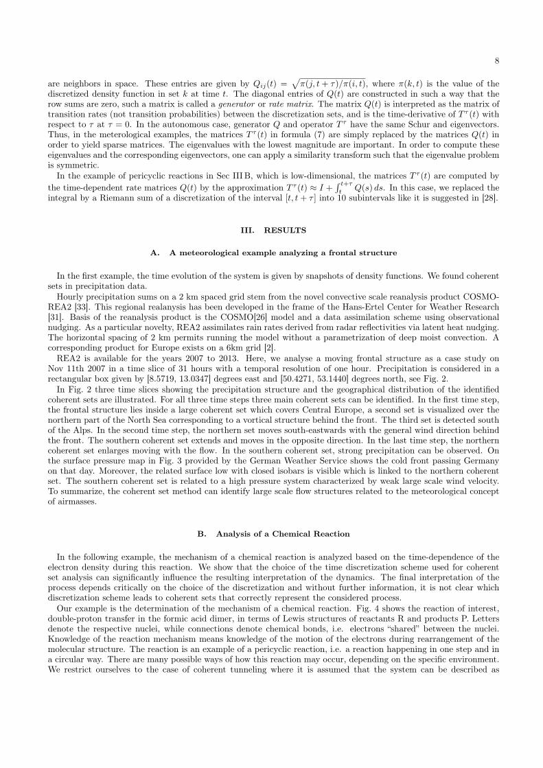
FIG. 4. Schematic drawing of double proton tunneling in the formic acid dimer. During the reaction from reactants R on theleft to products P on the right, the H nuclei attached to an O nuclei of one formic acid molecule move to the O nuclei ofthe other one. During that process the electron density also changes accordingly. The angle θ along which the radial electrondensity is measured is also shown.

a superposition of the lowest two (almost degenerate) states of the respective molecular Hamilton operator in thenon-relativistic approximation.

Typically, for small molecules like the formic acid dimer, it is possible to obtain the time-dependence of the electrondensity (the probability density of finding an electron at a certain location in space) for the reaction to a goodapproximation. However, to find the reaction mechanism, it is necessary to know the electronic flux density or currentdensity, a vector field that describes how the electrons move from one instant of time to the next. In contrast to theelectron density, the flux density is much harder to compute [1]. Hence, we investigate if an analysis of the time-dependent electron density alone with PCCA+ can be used to obtain information about the reaction mechanism,without explicit knowledge of the flux density.

For this purpose, we describe the tunneling process with a quantum mechanical two-state model similar to thatdescribed in [15]. The electronic structure of R is determined from a Hartree-Fock calculation with a cc-pVTZ basis set[20] using the program package Molpro,[36] and the program Orbkit[16] was used to calculate the electron density ofR. Although more advances methods for calculating the electronic structure of this molecule are available, the Hartree-Fock method suffices for the present purpose. The structure and electron density of P is given by the requirement ofconservation of angular momentum during the change from R to P. The time-dependence of the electron density isgiven analytically in the 2-state model. As the reaction is a cyclic rearrangement, we use cylindrical coordinates andconsider only the angular density, i.e. we integrate the electron density along all but the angular coordinate givenin Fig. 4. Then, the hope is that information about the reaction mechanism can be obtained from analyzing thedynamics of this angular density alone. For further details, see [28].

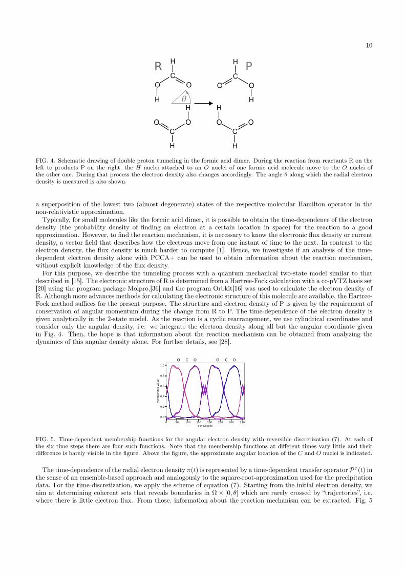
0 50 100 150 200 250 300 350 in Degree

0.0

0.2

0.4

0.6

0.8

1.0

mem

bers

hip

valu

e

O C O O C O

FIG. 5. Time-dependent membership functions for the angular electron density with reversible discretization (7). At each ofthe six time steps there are four such functions. Note that the membership functions at different times vary little and theirdifference is barely visible in the figure. Above the figure, the approximate angular location of the C and O nuclei is indicated.

The time-dependence of the radial electron density π(t) is represented by a time-dependent transfer operator Pτ (t) inthe sense of an ensemble-based approach and analogously to the square-root-approximation used for the precipitationdata. For the time-discretization, we apply the scheme of equation (7). Starting from the initial electron density, weaim at determining coherent sets that reveals boundaries in Ω × [0, θ] which are rarely crossed by “trajectories”, i.e.where there is little electron flux. From those, information about the reaction mechanism can be extracted. Fig. 5

11

shows the membership functions for this case together with the approximate angular position of the C and O nuclei.Two of the boundaries between membership functions correspond to angles where the C nuclei are located (θ = 90

and θ = 270), while the other two boundaries correspond to the center of the path connecting the initial and finalposition of the H nuclei (θ = 0 and θ = 180). Consequently, from this analysis we would conclude that there islittle electronic motion through the surfaces corresponding to these angles, implying a motion of the electrons suchthat they do not cross these surfaces.

0 50 100 150 200 250 300 350 in Degree

0.0

0.2

0.4

0.6

0.8

1.0

mem

bers

hip

valu

e

O C O O C O

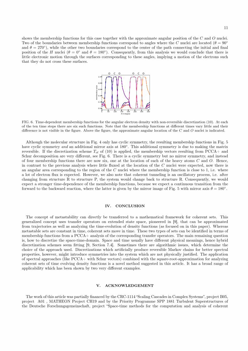
FIG. 6. Time-dependent membership functions for the angular electron density with non-reversible discretization (10). At eachof the ten time steps there are six such functions. Note that the membership functions at different times vary little and theirdifference is not visible in the figure. Above the figure, the approximate angular location of the C and O nuclei is indicated.

Although the molecular structure in Fig. 4 only has cyclic symmetry, the resulting membership functions in Fig. 5have cyclic symmetry and an additional mirror axis at 180. This additional symmetry is due to making the matrixreversible. If the discretization scheme Tol of (10) is applied, the membership vectors resulting from PCCA+ andSchur decomposition are very different, see Fig. 6. There is a cyclic symmetry but no mirror symmetry, and insteadof four membership functions there are now six, one at the location of each of the heavy atoms C and O. Hence,in contrast to the previous analysis where little fluxed at the location of the C nuclei were expected, now there isan angular area corresponding to the region of the C nuclei where the membership function is close to 1, i.e. wherea lot of electron flux is expected. However, we also note that coherent tunneling is an oscillatory process, i.e. afterchanging from structure R to structure P, the system would change back to structure R. Consequently, we wouldexpect a stronger time-dependence of the membership functions, because we expect a continuous transition from theforward to the backward reaction, where the latter is given by the mirror image of Fig. 5 with mirror axis θ = 180.

IV. CONCLUSION

The concept of metastability can directly be transferred to a mathematical framework for coherent sets. Thisgeneralized concept uses transfer operators on extended state space, pioneered in [9], that can be approximatedfrom trajectories as well as analyzing the time-evolution of density functions (as focused on in this paper). Whereasmetastable sets are constant in time, coherent sets move in time. These two types of sets can be identified in terms ofmembership functions from a PCCA+ analysis of the corresponding transfer operators. The main remaining questionis, how to discretize the space-time-domain. Space and time usually have different physical meanings, hence hybriddiscretization schemes seem fitting [9, Section 7.4]. Sometimes there are algorithmic issues, which determine thechoice of the approach used. Discretizations which artificially produce reversible Markov chains for better spectralproperties, however, might introduce symmetries into the system which are not physically justified. The applicationof spectral approaches (like PCCA+ with Schur vectors) combined with the square-root-approximation for analyzingcoherent sets of time evolving density functions is a novel method suggested in this article. It has a broad range ofapplicability which has been shown by two very different examples.

V. ACKNOWLEDGEMENT

The work of this article was partially financed by the CRC-1114 “Scaling Cascades in Complex Systems”, project B05,project A01 , MATHEON Project CH19 and by the Priority Programme SPP 1881 Turbulent Superstructures ofthe Deutsche Forschungsgemeinschaft, project “Space-time methods for the computation and analysis of coherent

12

families”.

[1] Ingo Barth, Hans-Christian Hege, Hiroshi Ikeda, Anatole Kenfack, Michael Koppitz, Jörn Manz, Falko Marquardt, andGuennaddi K. Paramonov. Concerted quantum effects of electronic and nuclear fluxes in molecules. Chemical PhysicsLetters, 481(1):118 – 123, 2009.

[2] C Bollmeyer, JD Keller, C Ohlwein, SWahl, S Crewell, P Friederichs, A Hense, J Keune, S Kneifel, I Pscheidt, et al. Towardsa high-resolution regional reanalysis for the european CORDEX domain. Quarterly Journal of the Royal MeteorologicalSociety, 141(686):1–15, 2015.

[3] Anton Bovier and Frank den Hollander. Metastability–A Potential-Theoretic Approach. Springer, 2015.[4] Gregory R Bowman, Vijay S Pande, and Frank Noé. An introduction to Markov state models and their application to long

timescale molecular simulation, volume 797. Springer Science & Business Media, 2013.[5] Alexander Bujotzek. Molecular Simulation of Multivalent Ligand-Receptor Systems. doctoral thesis, FU Berlin, 2013.[6] Carmen Chicone and Yuri Latushkin. Evolution semigroups in dynamical systems and differential equations. Number 70.

American Mathematical Soc., 1999.[7] P. Deuflhard and M. Weber. Robust Perron cluster analysis in conformation dynamics. Linear Algebra and its Applications,

161(184), 2005. 398 Special issue on matrices and mathematical biology.[8] Konstantin Fackeldey and Marcus Weber. GenPCCA – Markov state models for non-equilibrium steady states. Big data

clustering: Data preprocessing, variable selection, and dimension reduction. WIAS Report No. 29, pages 70 – 80, 2017.[9] G. Froyland and P. Koltai. Estimating long-term behavior of periodically driven flows without trajectory integration.

Nonlinearity, 30(5):1948, 2017.[10] Gary Froyland. An analytic framework for identifying finite-time coherent sets in time-dependent dynamical systems.

Physica D: Nonlinear Phenomena, 250:1–19, 2013.[11] Gary Froyland. Dynamic isoperimetry and the geometry of lagrangian coherent structures. Nonlinearity, 28(10):3587,

2015.[12] Gary Froyland and Kathrin Padberg-Gehle. Almost-Invariant and Finite-Time Coherent Sets: Directionality, Duration,

and Diffusion, pages 171–216. Springer New York, New York, NY, 2014.[13] Gary Froyland, Naratip Santitissadeekorn, and Adam Monahan. Transport in time-dependent dynamical systems: Finite-

time coherent sets. Chaos: An Interdisciplinary Journal of Nonlinear Science, 20(4):043116, 2010.[14] Cecilia Gonzalez-Tokman. Multiplicative ergodic theorems for transfer operators: towards the identification and analysis

of coherent structures in non-autonomous dynamical systems. Contemporary Mathematics, to appear.[15] Hans-Christian Hege, Jörn Manz, Falko Marquardt, Beate Paulus, and Axel Schild. Electron flux during pericyclic reactions

in the tunneling limit: Quantum simulation for cyclooctatetraene. Chemical Physics, 376(1):46 – 55, 2010.[16] Gunter Hermann, Vincent Pohl, Jean Christophe Tremblay, Beate Paulus, Hans-Christian Hege, and Axel Schild. Or-

bkit: A modular python toolbox for cross-platform postprocessing of quantum chemical wavefunction data. Journal ofComputational Chemistry, 37(16):1511–1520, 2016.

[17] Wilhelm Huisinga, Sean Meyn, and Christof Schütte. Phase transitions and metastability in markovian and molecularsystems. Annals of Applied Probability, pages 419–458, 2004.

[18] Wilhelm Huisinga and Bernd Schmidt. Metastability and Dominant Eigenvalues of Transfer Operators, pages 167–182.Springer Berlin Heidelberg, Berlin, Heidelberg, 2006.

[19] Itseez. Open source computer vision library. https://github.com/itseez/opencv, 2015.[20] Thom H. Dunning Jr. Gaussian basis sets for use in correlated molecular calculations. i. the atoms boron through neon

and hydrogen. The Journal of Chemical Physics, 90(2):1007–1023, 1989.[21] S. Klus, P. Koltai, and Ch. Schütte. On the numerical approximation of the Perron–Frobenius and Koopman operator.

Journal of Computational Dynamics, 3(1):51–79, 2016.[22] Peter Koltai, Giovanni Ciccotti, and Christof Schütte. On metastability and markov state models for non-stationary

molecular dynamics. J. Chem. Phys., 145:174103, 2016.[23] Susanna Kube and Marcus Weber. Preserving the Markov property of reduced reversible Markov chains. AIP Conference

Proceedings, 593(1048), 2008.[24] Han Cheng Lie, Konstantin Fackeldey, and Marcus Weber. A square root approximation of transition rates for a markov

state model. SIAM. J. Matrix Anal. Appl., 34:738–756, 2013.[25] Adam Nielsen. Computation Schemes for Transfer Operators. doctoral thesis, FU Berlin, 2016.[26] Consortium for small scale modelling, http:cosmo-model.org.[27] Martin K. Scherer, Benjamin Trendelkamp-Schroer, Fabian Paul, Guillermo Pérez-Hernández, Moritz Hoffmann, Nuria

Plattner, Christoph Wehmeyer, Jan-Hendrik Prinz, and Frank Noé. PyEMMA 2: A Software Package for Estimation,Validation, and Analysis of Markov Models. Journal of Chemical Theory and Computation, 11:5525–5542, October 2015.

[28] Axel Schild. Electron Fluxes During Chemical Processes in the Electronic Ground State. PhD thesis, Freie UniversitätBerlin, Berlin, 2013.

[29] Christof Schütte and Marco Sarich. Metastability and Markov State Models in Molecular Dynamics. Number 34 in CourantLecture Notes. American Mathematical Society, 2013.

13

[30] Christof Schütte and Han Wang. Building Markov state models for periodically driven non-equilibrium systems. Journalof Chemical Theory and Computation, 11(4):1819–1831, 2015.

[31] Clemens Simmer, Gerhard Adrian, Sarah Jones, Volkmar Wirth, Martin Göber, Cathy Hohenegger, Tijana Janjic, JanKeller, Christian Ohlwein, Axel Seifert, et al. Herz: The german hans-ertel centre for weather research. Bulletin of theAmerican Meteorological Society, 97(6):1057–1068, 2016.

[32] S. M. Ulam. A Collection of Mathematical Problems. Interscience Publisher NY, 1960.[33] Sabrina Wahl, Christoph Bollmeyer, Susanne Crewell, Clarissa Figura, Petra Friederichs, Andreas Hense, Jan D Keller,

and Christian Ohlwein. A novel convective-scale regional reanalyses COSMO-REA2: Improving the representation ofprecipitation. Meteorol. Z, 2017.

[34] Marcus Weber. Meshless Methods in Conformation Dynamics. doctoral thesis, FU Berlin, 2006.[35] Marcus Weber and Konstantin Fackeldey. GenPCCA: Spectral clustering for non-reversible Markov chains. ZIB Report

ZR-15-35, 2015.[36] H.-J. Werner, P. J. Knowles, G. Knizia, F. R. Manby, M. Schütz, et al. Molpro, version 2015.1, a package of ab initio

programs, 2015. see http://www.molpro.net.[37] Alper Yilmaz, Omar Javed, and Mubarak Shah. Object tracking: A survey. ACM Comput. Surv., 38(4), December 2006.