Journal of International Economics 108 (2017) 1–19

Contents lists available at ScienceDirect

Journal of International Economics

j ourna l homepage: www.e lsev ie r .com/ locate / j i e

From micro to macro: Demand, supply, and heterogeneity in thetrade elasticity�

Maria Basa, Thierry Mayerb,*, Mathias Thoenigc

aUniversity Paris 1 Panthéon-Sorbonne, Centre d′Economie de la Sorbonne (CES), Franceb Sciences Po, Banque de France, CEPII and CEPR 28, rue des Saints-Peres, 75007 Paris, Francec Faculty of Business and Economics, University of Lausanne and CEPR, Switzerland

A R T I C L E I N F O

Article history:Received 19 February 2016Received in revised form 5 May 2017Accepted 5 May 2017Available online xxxx

JEL classification:F1

Keywords:Trade elasticityFirm-level dataHeterogeneityGravityParetoLog-normal

A B S T R A C T

Models of heterogeneous firms with selection into export market participation generically exhibit aggregatetrade elasticities that vary across country-pairs. Only when heterogeneity is assumed Pareto-distributeddo all elasticities collapse into a unique elasticity, estimable with a gravity equation. This paper providesa theory-consistent methodology for quantifying country-pair specific aggregate elasticities when movingaway from Pareto, i.e. when gravity does not hold. Combining two firm-level customs datasets for which weobserve French and Chinese individual sales on the same destination market over the 2000–2006 period, weare able to estimate all the components of the bilateral aggregate elasticity: i) the demand-side parameterthat governs the intensive margin and ii) the supply side parameters that drive the extensive margin. Thesecomponents are then used to calculate theoretical predictions of bilateral aggregate elasticities over thewhole set of destinations, and how those elasticities decompose into different margins. Our predictions fitwell with econometric estimates, supporting our view that micro-data is a key element in the quantificationof aggregate trade elasticities.

© 2017 Elsevier B.V. All rights reserved.

1. Introduction

The response of trade flows to a change in trade costs, theaggregate trade elasticity, is a central element in any evaluation ofthe welfare impacts of trade liberalization. Arkolakis et al. (2012)recently showed that this parameter, let us call it e for the rest of thepaper, is actually one of the (only) two sufficient statistics neededto calculate Gains From Trade (GFT) under a surprisingly large set ofalternative modeling assumptions. Measuring those elasticities hastherefore been the topic of a long-standing literature in international

� This research has received funding from the European Research Council underthe European Community’s Seventh Framework Programme (FP7/2007–2013) GrantAgreement No. 313522. We thank the Editor and two anonymous referees for veryuseful remarks. The paper also benefited greatly at an early stage from commentsby David Atkin, Dave Donaldson, Swati Dhingra, Ben Faber, Pablo Fagelbaum, JeanImbs, Oleg Itskhoki, Jan de Loecker, Philippe Martin, Peter Morrow, Steve Redding,Andres Rodriguez Clare, Esteban Rossi-Hansberg, Katheryn Russ, Nico Voigtlander, andYoto Yotov, during presentations in UC Berkeley, UCLA, Penn State, Banque de France,WTO, CEPII, ISGEP in Stockholm, University of Nottingham, Banca d’Italia, PrincetonUniversity and CEMFI.

* Corresponding author.E-mail address: thierry.mayer@sciencespo.fr (T. Mayer).

economics. The most common practice (and the one recommendedby Arkolakis et al., 2012) is to estimate this elasticity in a macro-levelbilateral trade equation referred to as structural gravity in the lit-erature following the initial impulse by Anderson and van Wincoop(2003). In order for this estimate of e to be relevant for a particularexperiment of trade liberalization, it is crucial for this bilateral tradeequation to be correctly specified as a structural gravity model with,in particular, a unique elasticity to be estimated across country pairs.

Our starting point is that the model of heterogeneous firms withselection into export market participation (Melitz, 2003) will in gen-eral exhibit a bilateral-specific aggregate trade elasticity, i.e. an eni,which applies to each country pair, where i denotes the origin andn the destination of the flow. Only when heterogeneity is assumedPareto-distributed1 do all eni collapse to a single e. Under any other(commonly-used) distributional assumption, obtaining an estimateof the aggregate trade elasticity from a macro-level bilateral trade

1 Unless otherwise specified, Pareto is understood here as the unbounded versionused by most of the literature. See Helpman et al. (2008) and Melitz and Redding(2015) for results with the bounded version, where the trade elasticity recovers abilateral dimension.

http://dx.doi.org/10.1016/j.jinteco.2017.05.0010022-1996/© 2017 Elsevier B.V. All rights reserved.

2 M. Bas et al. / Journal of International Economics 108 (2017) 1–19

equation becomes problematic: first because a whole set of eni hasto be estimated, and second because structural gravity does nothold anymore. We argue that in this case quantifying trade elastic-ities at the aggregate level makes it necessary to use micro-levelinformation. To this purpose, we combine sales of French and Chi-nese exporters in many destination-product combinations for whichwe also observe the relevant tariff applied. We propose a theory-consistent methodology using this firm-level export data for quan-tifying all the components of the bilateral aggregate trade elasticity:i) the demand-side parameter that governs the intensive marginand ii) the supply side parameters that drive the extensive margin.These components are then assembled under theoretical guidanceto calculate the bilateral aggregate elasticities over the whole set ofdestinations.

Taking into account country pair heterogeneity in aggregate tradeelasticities is crucial for quantifying the expected impact of vari-ous trade policy experiments.2 Consider the example of envisionedTransatlantic or Transpacific trade agreements (TTIP or TPP). Underthe simplifying assumption of a unique elasticity, whether the tradeliberalization takes place with a proximate vs distant, large vs smalleconomy, is irrelevant in terms of trade-promoting effect or welfaregains calculations. By contrast, our results suggest that the relevanteni should be smaller (in absolute value) when trade liberalizationconcerns country-pairs where the volume of bilateral trade is alreadylarge. Regarding welfare, Head et al. (2014) and Melitz and Redding(2015) have shown theoretically that the GFT can be substantiallymis-estimated if one assumes a constant trade elasticity when the“true” elasticity is variable (the margin of error can exceed 100% inboth papers). The expected changes in trade patterns and welfareeffects of agreements such as TTIP or TPP will therefore be differentcompared to the unique elasticity case. One of the main objectivesof our paper is to quantify how wrong can one be when making pre-dictions based on a constant trade elasticity assumption. Naturally,this point also applies to the case of potential breakups of existingagreements such as the EU or NAFTA.

Our approach maintains the traditional CES (s) demand systemcombined with monopolistic competition. It features several stepsthat are structured around the following decomposition of the aggre-gate trade elasticity into the sum of the intensive margin and the(weighted) extensive margin:

eni = 1 − s︸ ︷︷ ︸intensive margin

+1

xni/xMINni︸ ︷︷ ︸mean-to-min

× d ln Nni

d ln tni︸ ︷︷ ︸extensive margin

. (1)

The weight is the inverse of the mean-to-min ratio, our observablemeasuring the dispersion of firm-level performance, that is definedas the ratio of average to minimum sales across markets. As themarket gets easier, the model predicts a larger presence of weakfirms, which augments productivity dispersion, captured by xni/xMINni .This lowers the weight of the extensive margin in the overall tradeelasticity, which is intuitive: in extremely easy markets, all poten-tial exporters should be active and the extensive margin of a smallchange in trade costs should be close to 0. When assuming Paretowith shape parameter h, the last part of the elasticity reduces to s −1−h, and the overall elasticity becomes constant and reflects only theparameter controlling dispersion in the distribution of productivity:eP

ni = eP = −h (Chaney, 2008). Without the Pareto assumption, one

2 Imbs and Méjean (2015) and Ossa (2015) recently argued that another source ofheterogeneity, the cross-sectoral one, raises important aggregation issues that mat-ter for aggregate outcomes of trade liberalization. We abstract from this particularkind of aggregation issue (which would reinforce the importance of heterogeneity foraggregate outcomes) in our paper and omit cross-sectoral variation in e until Section 6where we present industry-level estimates and use those to show that both demandand supply side determinants enter aggregate elasticities.

needs to calculate the two components of the aggregate elasticity(Eq. (1)). We do so in two steps.

Our first step aims to estimate the demand side parameter s

using firm-level exports. Since protection is imposed on all firmsfrom a given origin, higher demand and lower protection are notseparately identifiable when using only one exporting country. WithCES, firms are all faced with the same aggregate demand conditions.Thus, considering a second country of origin enables to isolate theeffects of trade policy, if the latter is discriminatory. We thereforecombine shipments by French and Chinese exporters to destinationsthat confront those firms with different levels of tariffs. Our setupyields a firm-level gravity equation which raises serious estimationchallenges. The main issue is the combination of a selection bias(inherent in any firm-level estimation of the Melitz (2003) model)with a very large set of fixed effects to be included in the regression.We use adapted versions of three estimators that have been pro-posed in the literature to deal with different aspects of the problem.Those three methods are evaluated with Monte Carlo simulationsof our theoretical setup, before being implemented on our data.Our preferred estimates of the firm-level trade elasticity imply anaverage value of (1 − s) around −4.

Our second and main step applies Eq. (1) and combines the esti-mate of the firm-level elasticity (1 − s) with the central supply sideparameter—reflecting dispersion in the distribution of productivity—to obtain theoretical predictions of the aggregate elasticities of totalexport, number of exporters and average exports per firm to eachdestination. Those predictions (one elasticity for each exporter-importer combination) require knowledge of the bilateral exportproductivity cutoff under which firms find exports to be unprofitable.We make use of the mean-to-min ratio to reveal those cutoffs. Akey element of our procedure is the calibration of the productivitydistribution. As an alternative to Pareto we consider the log-normaldistribution that fits the micro-data on firm-level sales very well.3

A related contribution of our paper is to discriminate betweenPareto and log-normal as potential distributions for the underlyingfirm-level heterogeneity, suggesting that log-normal does a betterjob at matching the non-unique response of exports to changes intrade costs. Two pieces of evidence in that direction are provided.The first provides direct evidence that aggregate trade elasticities arenon-constant across country pairs. The second is a strong correlationacross industries between firm-level and aggregate elasticities—atodds with the prediction of a null correlation under Pareto. Wealso find that the heterogeneity in trade elasticities is quantitativelyimportant: Although the average of bilateral elasticities is quite wellapproximated by a standard gravity model constraining the esti-mated parameter to be constant, deviations from this average levelcan be large. We show that under log-normal the eni are larger(in absolute value) for pairs with low volumes of trade. Hence thetrade-promoting impact of liberalization is expected to be larger forthis kind of trade partners. For Chinese exports, assuming a uniqueelasticity would underestimate the trade impact of a tariff liberaliza-tion by about 25% for countries with initially very small trade flows(Somalia, Chad or Azerbaijan for instance). By contrast, the errorwould be to overestimate by around 20% the exports created whenthe United States or Japan reduce their trade costs.

The next section relates our paper to the existing literature.Section 3 describes our model and empirical strategy. Section 4deals with the estimation challenges of the firm-level gravity regres-sions and reports the estimates of the intensive margin elasticity.

3 Head et al. (2014) provide evidence and references for several micro-level datasets that individual sales are much better approximated by a log-normal distributionwhen the entire distribution is considered (without left-tail truncation). Freund andPierola (2015) is a recent example showing, for all of the 32 countries used, very largedeviations from Pareto if the data is not vastly truncated to focus on the very largestfirms.

M. Bas et al. / Journal of International Economics 108 (2017) 1–19 3

Section 5 computes micro-based theoretical predictions of the bilat-eral aggregate elasticities and compares them to their gravity esti-mates obtained with Chinese and French aggregate export data.Section 6 investigates the implications of cross-industry heterogene-ity for our analysis and provides an additional piece of evidence infavor of non-constant aggregate trade elasticities. The final sectionconcludes.

2. Related literature

In the empirical literature estimating trade elasticities, differ-ent approaches and proxies for trade costs have been used, withan almost exclusive focus on aggregate country or industry-leveldata. The gravity approach to estimating those elasticities mostlyuses tariff data to estimate bilateral responses to variation in appliedtariff levels. Most of the time, identification is based on the cross-section of country pairs, with origin and destination determinantsbeing controlled through fixed effects (Hummels, 1999; Baier andBergstrand, 2001; Head and Ries, 2001; Romalis, 2007; Caliendo andParro, 2015 for instance). A related approach consists in using thefact that most foundations of gravity predict the same coefficienton trade costs and domestic cost shifters to estimate that elastic-ity from the effect on bilateral trade of exporter-specific changes inproductivity, export prices or exchange rates. Costinot et al. (2012)use industry-level data for OECD countries, and obtains a preferredelasticity of −6.53 relying on producer prices of the exporter asthe identifying variable.4 Our paper has consequences for how tointerpret those numbers in terms of underlying structural param-eters. With a homogeneous firms model of the Krugman (1980)type in mind, the estimated trade elasticity turns out to reveal ademand-side parameter only, 1 − s (this is also the case with Arm-ington differentiation and perfect competition as in Anderson andvan Wincoop, 2003). When instead considering heterogeneous firmsà la Melitz (2003), the literature has proposed that the aggregatetrade elasticity is driven solely by a supply-side parameter describ-ing the dispersion of the underlying distribution of firm productivity.This result has been shown with several demand systems (CES byChaney (2008), linear by Melitz and Ottaviano (2008), translog byArkolakis et al. (2010) for instance), but relies critically on the main-tained assumption of a Pareto distribution. The trade elasticity thenprovides an estimate of the dispersion parameter of the Pareto dis-tribution for firm productivity, h.5 We show here that both existinginterpretations of the estimated elasticities are too extreme: Whenthe Pareto assumption is relaxed, the aggregate trade elasticity is amix of demand and supply parameters.

A small set of papers estimate the intensive margin elasticity atthe exporter level. Berman et al. (2012) present estimates of the tradeelasticity with respect to real exchange rate variations across coun-tries and over time using firm-level data from France. Fitzgerald andHaller (2015) use firm-level data from Ireland, real exchange rate andweighted average firm-level applied tariffs as price shifters to esti-mate the trade elasticity. The results for the impact of real exchangerate on firms’ export sales are of a similar magnitude, around 0.8 to 1.

4 Other methodologies (also used for aggregate elasticities) use identification viaheteroskedasticity in bilateral flows, and have been developed by Feenstra (1994)and applied widely by Broda and Weinstein (2006) and Imbs and Méjean (2015). Yet,another alternative is to proxy trade costs using retail price gaps and their impact ontrade volumes, as proposed by Eaton and Kortum (2002) and extended by Simonovskaand Waugh (2011).

5 This result of a constant trade elasticity reflecting the Pareto shape holds whenmaintaining the CES demand system but making other improvements to the modelsuch as heterogeneous marketing and/or fixed export costs (Arkolakis, 2010; Eatonet al., 2011). In the Ricardian setup of Eaton and Kortum (2002), the tradeelasticity is also a (constant) supply side parameter reflecting heterogeneity, but thisheterogeneity takes place at the national level, and reflects the scope for comparativeadvantage.

Regarding tariffs, Fitzgerald and Haller (2015) construct a firm-leveldestination-year tariff as the weighted average of the applied tariffsat the product-destination-year level imposed on the firm’s products,using as weights the share of a product in firm total production. Theyfind a tariff elasticity ranging widely from −1.7 to −24 in their base-line table. The preferred estimate of Berthou and Fontagné (2016),who use the response of the largest French exporters in the UnitedStates to the levels of applied tariffs is −2.5. We depart from thosepapers by using an alternative methodology to identify the tradeelasticity with respect to applied tariffs; i.e. the differential treat-ment of exporters from two distinct countries (France and China) ina set of product-destination markets. We also describe thoroughlythe estimation challenges involved in firm-level gravity regressionsand provide the first rigorous evaluation of the alternative estimatorsavailable with Monte Carlo simulations using the canonical Melitz(2003) model as a Data Generating Process (DGP).

Our paper also relates to several recent papers studying patternsand consequences of heterogeneity in trade elasticities. Berman et al.(2012) and Gopinath and Neiman (2014) find that in order to predictcorrectly the aggregate patterns of trade adjustments to price shocks,one has to take into account firm-level heterogeneity with the useof micro-data. In both papers, heterogeneity matters because firmshave different individual responses in export and/or import behavior.In particular, both papers find that the firm-level elasticity dependsnegatively on the size of the firm (because of variable markups). Ourpaper also finds that measuring aggregate trade responses requiresusage of firm-level data. It is however for a different reason: Inour case, heterogeneity in aggregate trade elasticities simply origi-nates in a departure from the common assumption that productiveefficiency is Pareto-distributed.6 While we do recognize that tradeelasticities might differ across firms because of variable markups,our paper shows that this is not required to ensure that heterogene-ity matters for the aggregate economy and investigates a different,complementary, channel.7

We also contribute to the literature studying the importanceof the distributional assumption for firm heterogeneity for tradepatterns, trade elasticities and welfare. Head et al. (2014), Yang(2014), Melitz and Redding (2015) and Feenstra (2013) have recentlyargued that the simple gains from trade formula proposed byArkolakis et al. (2012) rely crucially on the Pareto assumption, whichmutes important channels of gains in the heterogenous firms case.Barba Navaretti et al. (2015) present gravity-based evidence that theexporting country fixed effects depends on characteristics of firms’distribution that go beyond the simple mean productivity, a fea-ture incompatible with the usually specified Pareto heterogeneity.Fernandes et al. (2015) use customs data for numerous developingcountries to show that a decomposition of total bilateral exportsinto intensive and extensive margins exhibits an important role forthe former, with patterns consistent with log-normally distributedheterogeneity and incompatible with (unbounded) Pareto. The alter-natives to Pareto considered to date in welfare gains quantification

6 Yet another alternative source of bilateral heterogeneity in the trade elastic-ity could be a composition effect, coming from aggregating products with differentunderlying elasticities, or comparing pairs with different country characteristics. Ourempirical analysis showing heterogeneous elasticities at the aggregate level is basedon a ratio approach that conditions on the two exporting countries having the sameset of destination-product combinations.

7 A further interesting result is that heterogeneous firm-level elasticities do notguarantee variable bilateral aggregate trade elasticities. Melitz and Ottaviano (2008)and Berman et al. (2012) are two examples of models with variable markups that yieldheterogeneity in firm-level response to trade costs. However, in both cases, when pro-ductivity is assumed Pareto-distributed, the bilateral aggregate trade elasticity turnsout to be a constant only related to the Pareto shape parameter. Introducing variablemarkups in the Pareto context therefore is not sufficient to generate the data patternswe uncover here.

4 M. Bas et al. / Journal of International Economics 108 (2017) 1–19

exercises are i) the bounded Pareto by Helpman et al. (2008), Melitzand Redding (2015) and Feenstra (2013), ii) the log-normal by Headet al. (2014), Fernandes et al. (2015) and Yang (2014), and iii) amixture of Pareto and log-normal in Nigai (2017). A key simplify-ing feature of Pareto is to yield a constant trade elasticity, whichis not the case for alternative distributions. Helpman et al. (2008),Novy (2013) and Spearot (2013) have produced empirical evidenceshowing substantial variation in the trade cost elasticity across coun-try pairs. Our contribution to that literature is to use the estimateddemand and supply-side parameters to construct predicted bilateralelasticities for aggregate flows under the log-normal assumption,and compare their first moments to gravity-based estimates. Itshould be noted that there are other ways to generate bilateraltrade elasticities. The most obvious is to depart from the simple CESdemand system. Novy (2013) builds on Feenstra (2003), using thetranslog demand system with homogeneous firms to obtain variabletrade elasticities. Spearot (2013) obtains country-pair specific tradeelasticities motivated by the Melitz and Ottaviano (2008) model,which combines firm heterogeneity with a linear demand system.Atkeson and Burstein (2008) maintain CES demand, generating het-erogeneity in elasticities through oligopoly. We choose here to keepthe change with respect to the benchmark Melitz/Chaney frame-work to a minimal extent, keeping CES and monopolistic competi-tion, while changing only the distributional assumption, comparingPareto to log-normal.8

3. Firm-level and aggregate-level trade elasticities: theory

We use the multi-country one-sector version of the Melitz (2003)theoretical framework. Country i hosts a set of heterogeneous firmsfacing a constant price elasticity (CES utility combined with icebergcosts) and contemplating exports to several destinations indexed bysubscript n. In this setup, firm-level export value x depends uponthe firm-specific unit input requirement (a), wages at home (wi),and real expenditure in n, An ≡ XnPs−1

n , with Pn the ideal CES priceindex relevant for sales in n. An is a measure of “attractiveness” ofmarket n (expenditure discounted by the degree of competition inthis market). There are trade costs associated with reaching marketn, consisting of an observable iceberg-type part (tni), and a shockthat affects firms differently on each market, bni(a).9 Monopolis-tic competition ensures a complete pass-through of trade costs intodelivered prices, such that firm-level sales are

xni(a) =(

s

s − 1

)1−s

[awitnibni(a)]1−sAn. (2)

The firm-level trade elasticity, i.e. the individual reaction of xni to achange in observable trade costs, is 1 − s .

In order to obtain the aggregate trade elasticity, we start by sum-ming, for each country pair, the sales Eq. (2) across all active firms:

Xni = Vni ×(

s

s − 1

)1−s

(witni)1−sAnMe

i , (3)

8 Relying on the same approach (CES and monopolistic competition), Helpman etal. (2008) assume bounded Pareto to obtain bilateral trade elasticities that vary acrosscountry pairs. They estimate the distance trade elasticity at the aggregate level, whilein this paper, we estimate directly the price elasticity using tariff data and we usefirm-level information.

9 An example of such unobservable term would be the presence of workers fromcountry n in firm a, that would increase the internal knowledge on how to reachconsumers in n, and therefore reduce trade costs for that specific company in that par-ticular market (b being a mnemonic for barrier to trade). Note that this type of randomtrade cost shock is isomorphic to assuming a firm-destination demand shock in thisCES-monopolistic competition model.

where Mei is the mass of entrants and Vni is a term which denotes

a cost-performance index of exporters located in country i andselling in n. This index, introduced by Helpman et al. (2008), isdefined as

Vni ≡∫ a∗

ni

0a1−sg(a)da, (4)

where a ≡ a × b(a) corresponds to the unitary labor requirementrescaled by the firm-destination shock and g(.) denotes its PDF (witha corresponding CDF denoted by G(.)). In Eq. (4), a∗

ni is the rescaledlabor requirement of the firm that just breaks even and thereforeexports to market n. The solution for this cutoff firm is the costsatisfying the zero profit condition, i.e., xni(a∗

ni) = swi fn, where fn isthe fixed export cost in each destination n. Using Eq. (2), this cutoffis characterized by

a∗ni =

s − 1s

1

tni f 1/(s−1)n

(An

swsi

) 1s−1

. (5)

We are interested in the (partial) elasticity of aggregate trade valuewith-respect to variable trade costs, tni. Partial means here holdingconstant origin-specific and destination-specific terms (income andprice indices) as in Arkolakis et al. (2012) and Melitz and Redding(2015).10 Using Eq. (3), we obtain the bilateral aggregate tradeelasticity:

eni ≡ d ln Xni

d ln tni= 1 − s − cni, (6)

which uses the fact that d ln a∗ni/d ln tni = −1. The cni term, intro-

duced by Arkolakis et al. (2012), describes how Vni varies with anincrease in the cutoff cost a∗

ni, that is an easier access of marketn for firms in i:

cni ≡ d ln Vni

d ln a∗ni

=a∗2−s

ni g(a∗

ni

)Vni

. (7)

Eqs. (6) and (7) show that the aggregate trade elasticity should,in general, not be constant across country pairs. They also makeit clear that the aggregate elasticity is a combination of the firm-level trade elasticity, 1 − s , and the contribution to total exportchanges due to entry and exit of firms into the export market,cni.

In order to evaluate eni, combining Eq. (7) with Eq. (4) reveals thatwe need to know the value of bilateral cutoffs a∗

ni. In order to obtainthose, we define the following expression

H(a∗ni) ≡ 1

a∗1−sni

∫ a∗ni

0a1−s g(a)

G(a∗

ni

) da =Vni

a∗1−sni G

(a∗

ni

) , (8)

a monotonic, invertible function with a parametrization that istightly linked to the distributional assumptions retained for G(.) (seeEq. (20) in Section 5.1). In this model, H(.) has a straightforwardeconomic interpretation. It is the ratio of average over minimum per-formance (measured as a*1−s ) of firms located in i and exporting ton. Using Eqs. (2) and (3) reveals that this ratio also corresponds to theobserved mean-to-min ratio of sales:

H(a∗ni) =

xni

xni(a∗

ni

) =xni

xMINni. (9)

10 In practical terms, the use of importer and exporter fixed effects in gravityregressions (the main source of estimates of the aggregate elasticity) holds wi ,Me

i and An constant when estimating Eq. (3).

M. Bas et al. / Journal of International Economics 108 (2017) 1–19 5

In firm-level export data sets, the ratio of average to minimum tradeflows by firm in each destination country n is an observable. UsingEq. (9), one can reveal â∗

ni, the predicted value of the export cutoff fori firms exporting to n as a function of the mean-to-min ratio of salesin each destination market:

â∗ni = H−1

(xni

xMINni

). (10)

Equipped with the bilateral cutoff, we use Eqs. (6) to (9) to quantifythe bilateral aggregate trade elasticity

eni = 1 − s − xMINni

xn,i× â∗

nig(â∗

ni

)G

(â∗

ni

) , (11)

where (1 − s) is obtained from the firm-level export equation (seeSection 4). We also calculate two other aggregate elasticities: theelasticity of the number of exporters Nni (the so-called extensivemargin) and the elasticity of average exports per firm xni. The num-ber of active exporters is closely related to the cutoff since Nni =Me

i × G(a∗

ni

), where Me

i represents the mass of entrants. Differentiat-ing and using Eq. (11) we can calculate the bilateral extensive marginof trade

d ln Nni

d ln tni= − â∗

nig(â∗

ni

)G

(â∗

ni

) . (12)

From the accounting identity Xni ≡ Nni × xni, we obtain the (partial)elasticity of average exports per firm to trade simply as the differ-ence between the predicted aggregate elasticity, Eq. (11) and thepredicted extensive margins, Eq. (12):

d ln xni

d ln tni= eni − d ln Nni

d ln tni= 1 − s − â∗

nig(â∗

ni

)G

(â∗

ni

) (xMINni

xn,i− 1

). (13)

Combining Eqs. (11) and (12), we can re-express aggregate elastici-ties as a function of the intensive and extensive margins and of themean-to-min ratio:

eni = 1 − s︸ ︷︷ ︸intensive margin

+

weighted extensive margin︷ ︸︸ ︷1

xni/xMINni︸ ︷︷ ︸mean-to-min

× d ln Nni

d ln tni︸ ︷︷ ︸extensive margin

, (14)

which is Eq. (1) presented in the Introduction 1. This decompositionshows that the aggregate trade elasticity is the sum of the inten-sive margin and of the (weighted) extensive margin. The weight onthe extensive margin depends only on the mean-to-min ratio, anobservable measuring the dispersion of relative firm performance(H(a∗

ni) in the model). Intuitively, the weight of the extensive mar-gin should be decreasing when the market gets easier. Indeed easymarkets have higher rates of entry, G(a∗), and therefore increasingpresence of weaker firms which augments dispersion measured asH

(a∗

ni

). The marginal entrant in an easy market will therefore have

less influence on aggregate exports, a smaller impact of the exten-sive margin. In the limit, the weight of the extensive margin becomesnegligible and the whole of the aggregate elasticity is due to theintensive margin/demand parameter. In the (unbounded) Pareto casehowever, this mechanism is not operational since H

(a∗

ni

)and there-

fore the weight of the extensive margin is constant. In Section 5,we implement our method with both Pareto-distributed a as well aswith log-normally-distributed a (which yields a varying dispersionof sales across destinations).

There are two major elements needed for the practical implemen-tation of Eq. (14). First, we need to obtain an estimate of 1 − s , the

parameter relevant in the firm-level trade elasticity. This is the topic ofSection 4. Second, we need to measure the mean-to-min ratio, H(a∗

ni),in the weighted extensive margin that add to the firm-level elastic-ity to yield the response of total trade to a change in trade costs. Thisis done in Section 5. Our framework until now has been silent aboutthe product/sector dimension. However, our data (export values andtariffs notably) come with product information, and it is possible thatdifferent products (we index those with p) are characterized by differ-ent values of the demand elasticity s and/or of the dispersion of firmperformance, H

(a∗

ni

). The composition effects coming from such dis-

persion in sectoral characteristics has been well documented in therecent work by Imbs and Méjean (2015) and Ossa (2015) for instance.We want to first present results that abstract from this dimension andfocus on the new source of bilateral heterogeneity we propose: theone coming “purely” from distributional assumptions. In Sections 4and 5, we therefore abstract from cross-sectoral heterogeneity in s

and in H(a∗

ni

). Those should be understood as averages of the under-

lying sectoral values, which we obtain by pooling over sectors. Thisoffers the advantage of compactness in the presentation of results.In Section 6, we return to that sectoral issue and let all structuralparameters and observables take a different value across sectors inour computation of firm-level and aggregate elasticities.

4. Estimation of the firm-level trade elasticity

4.1. Estimation challenges

Three serious methodological challenges arise when estimatingthe firm-level response of export values to variation in tariffs whilekeeping a close link to theory.

4.1.1. The need for multiple originsThe first challenge is to separate the effect of trade costs from

destination fixed effects. At this stage, it is useful to account forthe product (p) dimension for which we observe both the valueexported by the firm, xp

ni(a), and the bilateral tariff rate tpni(a). Trade

costs include both tariffs and other trade costs (distance Dni forinstance), and we assume the standard functional form such thatt

pni =

(1 + tp

ni

)Dd

ni. From now on, we will use the term “market”to designate a product-destination combination. Taking logs of the

demand Eq. (2), where 4pni(a) ≡

(bp

ni(a))1−s

is our unobservablefirm-market error term, a “firm-level gravity” equation is obtained:

ln xpni(a) =(1− s) ln

(s

s − 1

)+ (1 − s) ln(awi)+ (1 − s) ln

(1 + tp

ni

)+ (1 − s)d ln Dni + ln Ap

n + ln 4pni(a). (15)

The objective is to estimate 1 −s out of the impact of tariffs on firm-level sales. At this stage of the paper, as discussed above, we considera unique s , which can be interpreted as an average of elasticities thatmight vary across products. We will come back to industry-specificelasticities in Section 6. In the gravity literature, it has become com-mon practice to capture Ap

n (a complex construction, that dependsnon-linearly upon s) with market fixed effects. This is however notapplicable if the data set at hand covers only one origin country,since Ap

n and tpn would then vary across the same dimensions.11 To

11 Most if not all papers estimating firm-level gravity rely on only one source ofexport flows, while still estimating the impact of exchange rate (Berman et al., 2012),tariffs (Berthou and Fontagné, 2016) or both (Fitzgerald and Haller, 2015). The identi-fication in those papers then comes from another dimension, usually time. However,this strategy requires making the assumption that XnPs−1

n does not vary over timewhen tn does. This is inconsistent with a theory where trade costs enter the priceindex. Also the time dimension of variance in tariffs might be problematic sinceFitzgerald and Haller (2015) note that the changes in tariffs over time are small relativeto the cross-sectional variations.

6 M. Bas et al. / Journal of International Economics 108 (2017) 1–19

remain theory-consistent, one therefore needs to use at least twosets of exporters, based in countries that face different levels of tar-iffs applied by n. We do combine firm-level customs data for Franceand China (i = [FR, CN]), where the value of export flows is availableat the firm–HS6–destination level in each year. We measure bilateraltariffs tp

ni using WITS at the HS6–destination country level in eachyear. Proxies for Dni include distance, contiguity, colonial linkageand common language all obtained from the CEPII gravity database.Section 4.2 gives more detail about each of those data sources.

4.1.2. The fixed effects curseThe second challenge relates to the number of fixed effects to

be estimated. In addition to the market dimension (Apn), we need a

set of fixed effects at the firm level to capture marginal costs (awi)(and more generally all other unobservable firm-level determinantsof export performance, such as quality of products exported, man-agerial capabilities. . . ). Since there are tens of thousands of exportersin each origin country and several hundred thousand destination–product combinations, the Least Square Dummy Variable–bruteforce-approach is not feasible. There are two alternative imple-mentable solutions that we consider. The first solution is to estimateEq. (15) directly using the high-dimensional procedure that wasdeveloped by labor economists to deal with the very large number offixed effects implied by employer–employee data. 12

ln xpni(a) = FEa

i +FEpn +(1−s) ln(1+tp

ni)+(1−s)d ln Dni +ln 4pni(a).

(16)

We call this approach two-way fixed effects procedure, 2WFE, sincewe have two dimensions of unobserved heterogeneity to be con-trolled for (i.e. firm fixed effects FEa

i and market fixed effects FEpn).

The second solution is a ratio-type estimation inspired by Hallak(2006), Romalis (2007), Head et al. (2010), and Caliendo and Parro(2015) that removes observable and unobservable determinants forboth firm-level and destination factors. This method uses four indi-vidual export flows to calculate ratios of ratios: an approach referredto as Tetrads from now on. Consider a given French firm j and aChinese firm � exporting to both n and a reference country k. TheIndependence of Irrelevant Alternatives (IIA) property of the CESdemand system allows to manipulate Eq. (2) to write the followingTetrad:

xpn(aj,FR )/xp

k(aj,FR )

xpn(a

�,CN )/xpk(a

�,CN )=

(tp

nFR/tp

kFR

tpnCN/tp

kCN

)1−s

× 4pn(aj,FR )/4p

k(aj,FR )

4pn(a

�,CN )/4pk(a

�,CN ). (17)

Denoting tetradic terms with a ∼ symbol, one can re-write Eq. (17) asan estimable equation

ln xp{j,n,k} = (1 − s) ln

˜(1 + tp

{n,k})

+ (1 − s)d ln D{n,k} + ln 4p{j,n,k}. (18)

This approach involves a linear regression of log “tetraded” flows onlog “tetraded” trade costs and does not require the estimation of anyfixed effect. This method is therefore very simple computationally. Italso lends itself easily to graphical analysis and will finally provide anatural test of non-constant aggregate elasticities, which we conductin Section 5.3.

4.1.3. Firm-level zeroes (selection bias)The third challenge is to account for the selection of firms into dif-

ferent export markets. Assuming that fixed export costs vary across

12 The fastest procedure to date available in Stata, reghdfe, has been developed bySergio Correia building on Guimarães and Portugal (2010).

markets and are paid using labor of the origin country, profits inthis setup are given by xp

ni(a)/s − wi f pn . From Eq. (15), we see that

a firm with a low cost (awi) can afford having a low draw on 4pni(a)

and still export profitably to n. The same logic applies for large (highAp

n), and easy to reach (low tpni) markets. Concerning our variable of

interest, higher tariff observations will be associated with firms hav-ing drawn higher 4p

ni(a), thus biasing downwards our estimate of thetrade elasticity. The solution to this selection bias is not trivial in ourcase where a large set of fixed effects is included. Although we areunaware of a “perfect” estimator, we propose three alternative meth-ods, that we confront to Monte Carlo evidence of a simulated versionof the model.

First, one can focus the regressions on firms that have such a largeproductivity that their idiosyncratic destination shock is of secondorder. Inspired by Mulligan and Rubinstein (2008), Paravisini et al.(2015) and Fitzgerald and Haller (2015), we concentrate the analysison large firms that serve almost all markets. This requires to decideon a variable likely to predict small levels of selection. Paravisini etal. (2015) use firm-level measures of total exports and credit, whileFitzgerald and Haller (2015) use a threshold of firm-level employ-ment. We implement this approach with our data by restricting thesample to the largest exporter in each origin-product. Because thisapproach can accommodate our two-way fixed effects procedure(firm and destination) very easily, we call it 2WFE on top exporters.The second estimator relies upon the Tetrads method, with a similarstrategy of restricting attention to large exporting firms that are theleast likely to be affected by the selection bias. When taking ratiosof ratios of individual trade flows, we focus on the top exporters ofeach country,13 and look at their relative exports in different markets(compared to a reference country). We expect those two methods togive comparable results. The issue with both estimators is that theyestimate the firm-level trade elasticity on a reduced sub-sample ofthe largest firms. Those might have different trade elasticities, forreasons outside of our model.14 Our third estimator reinstates thefull sample of exporters. Assuming a normally distributed ln 4

pni(a) in

Eq. (15) yields a generalized structural Tobit, that we will refer to asEK-Tobit, since it was developed by Eaton and Kortum (2001). Crozetet al. (2012) apply EK-Tobit to the heterogeneous exporter model byusing the theoretical equation for minimum sales, xp,MIN

ni (a) = swi f pn ,

which therefore provides a natural estimate for the truncation pointfor each market. EK-Tobit is the best estimator for our theoreticalframework, with an important caveat: We must reduce the numberof included fixed effects because it seems computational unfeasibleto estimate a generalized Tobit with the very large set of fixed effectsour theory demands.15

We therefore have three possible estimators, 2WFE on topexporters, Tetrads on top exporters, and EK-Tobit. We now proceed totest for the performance of our three imperfect estimators meant tocorrect for the selection bias using Monte Carlo simulations. The DGPuses Eq. (15) for the value xni(a) exported by 100,000 firms dividedinto two origin countries and selling in 80 (to roughly match the num-bers we have in our sample). The true value of s is set to 5. The fixedexport costs fn and the market size An are drawn from independentlog-normal distributions calibrated to generate the same proportion

13 j and � are chosen as the top exporters to k in value terms in Eq. (17).14 Berman et al. (2012) show that several models featuring variable markups predict

that large firms should face lower demand elasticities and therefore react less thansmall firms to a change in trade costs. Their finding that the response to exchange ratechanges declines with productivity (confirmed by Chatterjee et al. (2013) for Brazilianexporters and Li et al. (2015) for Chinese exporters) suggests that the estimates in thepresent paper could be considered as a lower bound.15 Although Greene (2004) shows that the Tobit model is much less subject to the

incidental parameters problem than other non-linear models such as logit or probit,it is not possible to include the very large number of fixed effects in the EK-Tobitmodel due to computational burden. We also detect no sign of bias in our Monte Carlosimulations.

M. Bas et al. / Journal of International Economics 108 (2017) 1–19 7

(b) Chinese firms in Japan(a) French firms in Belgium

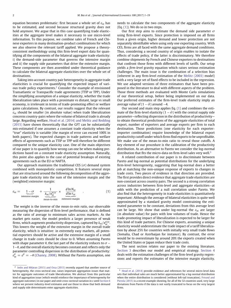
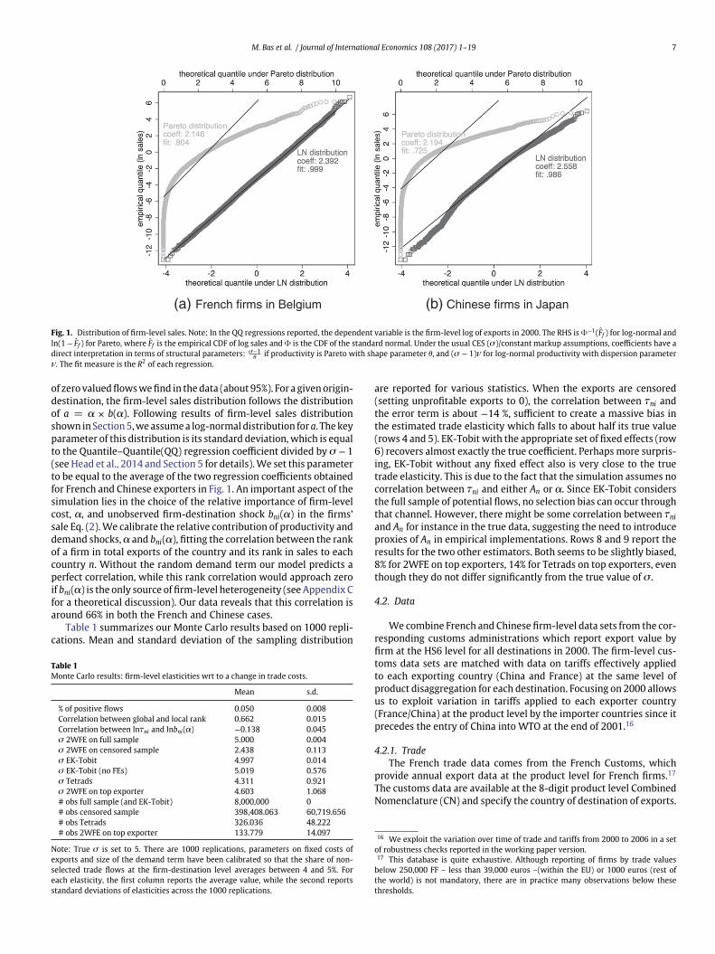
Fig. 1. Distribution of firm-level sales. Note: In the QQ regressions reported, the dependent variable is the firm-level log of exports in 2000. The RHS is V−1(Ff ) for log-normal andln(1 − Ff ) for Pareto, where Ff is the empirical CDF of log sales and V is the CDF of the standard normal. Under the usual CES (s)/constant markup assumptions, coefficients have adirect interpretation in terms of structural parameters: s−1

h if productivity is Pareto with shape parameter h, and (s − 1)m for log-normal productivity with dispersion parameterm. The fit measure is the R2 of each regression.

of zero valued flows we find in the data (about 95%). For a given origin-destination, the firm-level sales distribution follows the distributionof a = a × b(a). Following results of firm-level sales distributionshown in Section 5, we assume a log-normal distribution for a. The keyparameter of this distribution is its standard deviation, which is equalto the Quantile–Quantile(QQ) regression coefficient divided by s − 1(see Head et al., 2014 and Section 5 for details). We set this parameterto be equal to the average of the two regression coefficients obtainedfor French and Chinese exporters in Fig. 1. An important aspect of thesimulation lies in the choice of the relative importance of firm-levelcost, a, and unobserved firm-destination shock bni(a) in the firms’sale Eq. (2). We calibrate the relative contribution of productivity anddemand shocks, a and bni(a), fitting the correlation between the rankof a firm in total exports of the country and its rank in sales to eachcountry n. Without the random demand term our model predicts aperfect correlation, while this rank correlation would approach zeroif bni(a) is the only source of firm-level heterogeneity (see Appendix Cfor a theoretical discussion). Our data reveals that this correlation isaround 66% in both the French and Chinese cases.

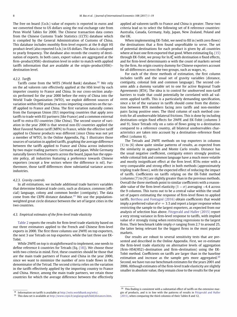
Table 1 summarizes our Monte Carlo results based on 1000 repli-cations. Mean and standard deviation of the sampling distribution

Table 1Monte Carlo results: firm-level elasticities wrt to a change in trade costs.

Mean s.d.

% of positive flows 0.050 0.008Correlation between global and local rank 0.662 0.015Correlation between lntni and lnbni(a) −0.138 0.045s 2WFE on full sample 5.000 0.004s 2WFE on censored sample 2.438 0.113s EK-Tobit 4.997 0.014s EK-Tobit (no FEs) 5.019 0.576s Tetrads 4.311 0.921s 2WFE on top exporter 4.603 1.068# obs full sample (and EK-Tobit) 8,000,000 0# obs censored sample 398,408.063 60,719.656# obs Tetrads 326.036 48.222# obs 2WFE on top exporter 133.779 14.097

Note: True s is set to 5. There are 1000 replications, parameters on fixed costs ofexports and size of the demand term have been calibrated so that the share of non-selected trade flows at the firm-destination level averages between 4 and 5%. Foreach elasticity, the first column reports the average value, while the second reportsstandard deviations of elasticities across the 1000 replications.

are reported for various statistics. When the exports are censored(setting unprofitable exports to 0), the correlation between tni andthe error term is about −14 %, sufficient to create a massive bias inthe estimated trade elasticity which falls to about half its true value(rows 4 and 5). EK-Tobit with the appropriate set of fixed effects (row6) recovers almost exactly the true coefficient. Perhaps more surpris-ing, EK-Tobit without any fixed effect also is very close to the truetrade elasticity. This is due to the fact that the simulation assumes nocorrelation between tni and either An or a. Since EK-Tobit considersthe full sample of potential flows, no selection bias can occur throughthat channel. However, there might be some correlation between tni

and An for instance in the true data, suggesting the need to introduceproxies of An in empirical implementations. Rows 8 and 9 report theresults for the two other estimators. Both seems to be slightly biased,8% for 2WFE on top exporters, 14% for Tetrads on top exporters, eventhough they do not differ significantly from the true value of s .

4.2. Data

We combine French and Chinese firm-level data sets from the cor-responding customs administrations which report export value byfirm at the HS6 level for all destinations in 2000. The firm-level cus-toms data sets are matched with data on tariffs effectively appliedto each exporting country (China and France) at the same level ofproduct disaggregation for each destination. Focusing on 2000 allowsus to exploit variation in tariffs applied to each exporter country(France/China) at the product level by the importer countries since itprecedes the entry of China into WTO at the end of 2001.16

4.2.1. TradeThe French trade data comes from the French Customs, which

provide annual export data at the product level for French firms.17

The customs data are available at the 8-digit product level CombinedNomenclature (CN) and specify the country of destination of exports.

16 We exploit the variation over time of trade and tariffs from 2000 to 2006 in a setof robustness checks reported in the working paper version.17 This database is quite exhaustive. Although reporting of firms by trade values

below 250,000 FF – less than 39,000 euros –(within the EU) or 1000 euros (rest ofthe world) is not mandatory, there are in practice many observations below thesethresholds.

8 M. Bas et al. / Journal of International Economics 108 (2017) 1–19

The free on board (f.o.b.) value of exports is reported in euros andwe converted those to US dollars using the real exchange rate fromPenn World Tables for 2000. The Chinese transaction data comesfrom the Chinese Customs Trade Statistics (CCTS) database whichis compiled by the General Administration of Customs of China.This database includes monthly firm-level exports at the 8-digit HSproduct-level (also reported f.o.b.) in US dollars. The data is collapsedto yearly frequency. The database also records the country of desti-nation of exports. In both cases, export values are aggregated at thefirm–product(HS6)–destination level in order to match with appliedtariffs information that are available at the origin–product(HS6)–destination level.

4.2.2. TariffsTariffs come from the WITS (World Bank) database.18 We rely

on the ad valorem rate effectively applied at the HS6 level by eachimporter country to France and China. In our cross-section analy-sis performed for the year 2000 before the entry of China into theWorld Trade Organization (WTO), we exploit different sources ofvariation within HS6 products across importing countries on the tar-iff applied to France and China. The first variation naturally comesfrom the European Union (EU) importing countries that apply zerotariffs to trade with EU partners (like France) and a common externaltariff to extra-EU countries (like China). The second source of vari-ation in the year 2000 is that several non-EU countries applied theMost Favored Nation tariff (MFN) to France, while the effective tariffapplied to Chinese products was different (since China was not yeta member of WTO). In the Online Appendix, Fig. 1 illustrates thosesources of variation in applied tariffs, graphing the average differencebetween the tariffs applied to France and China across industriesby two major trading partners: Germany and Japan. While Germanynaturally favors French exports across the board, Japan has the oppo-site policy, all industries featuring a preference towards Chineseexporters (except a few sectors where the difference is nil). Fur-thermore, those tariff differences show substantial variance acrossindustries.

4.2.3. Gravity controlsIn all estimations, we include additional trade barriers variables

that determine bilateral trade costs, such as distance, common (offi-cial) language, colony and common border (contiguity). The datacome from the CEPII distance database.19 We use the population-weighted great circle distance between the set of largest cities in thetwo countries.

4.3. Empirical estimates of the firm-level trade elasticity

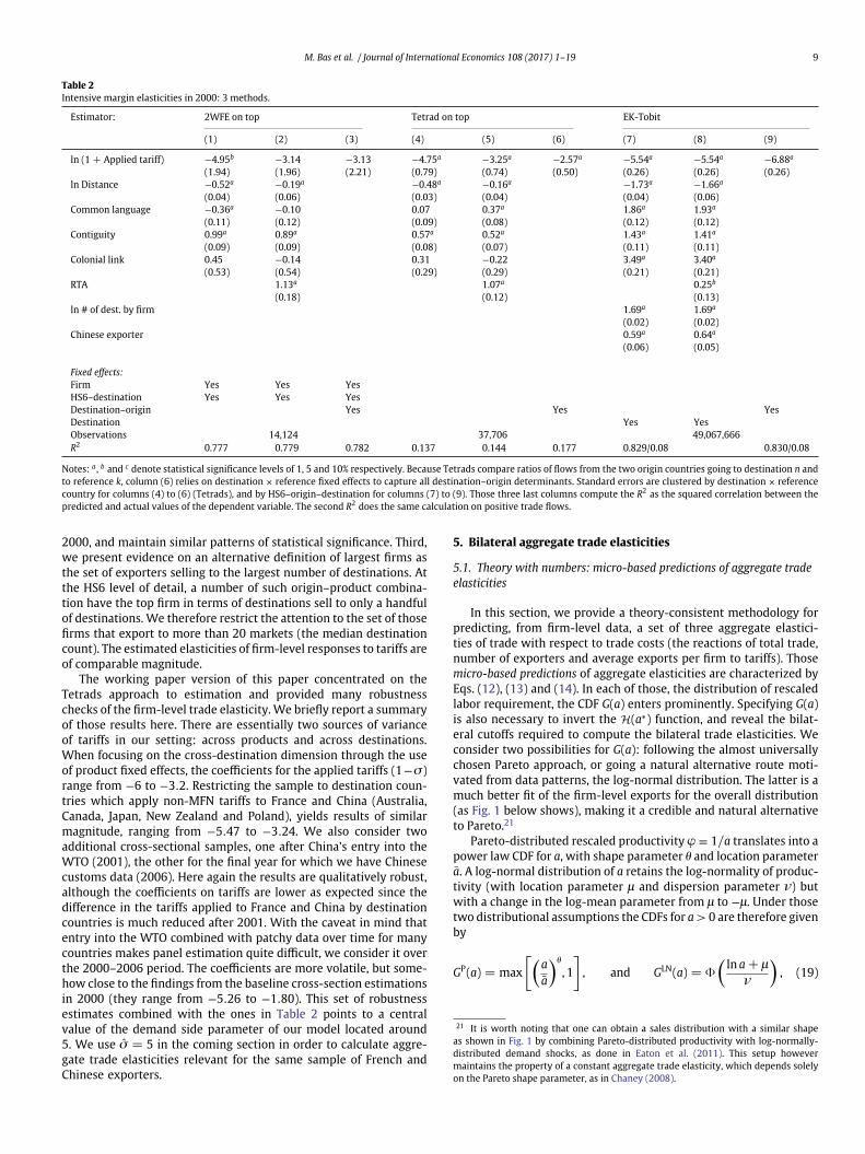
Table 2 reports the results for firm-level trade elasticity based onour three estimators applied to the French and Chinese firm-levelexports in 2000. The first three columns use 2WFE on top exporters,the next 3 use Tetrads on top exporters, while the last three use EK-Tobit.

While 2WFE on top is straightforward to implement, one needs todefine reference k countries for Tetrads (Eq. (18)). We choose thosewith two criteria in mind. First, these countries should be those thatare the main trade partners of France and China in the year 2000,since we want to minimize the number of zero trade flows in thedenominator of the Tetrad. The second criteria relies on the variationin the tariffs effectively applied by the importing country to Franceand China. Hence, among the main trade partners, we retain thosecountries for which the average difference between the effectively

18 Information on tariffs is available at http://wits.worldbank.org/wits/.19 This data set is available at http://www.cepii.fr/anglaisgraph/bdd/distances.htm.

applied ad valorem tariffs to France and China is greater. These twocriteria lead us to select the following set of 8 reference countries:Australia, Canada, Germany, Italy, Japan, New Zealand, Poland andthe UK.

When implementing EK-Tobit, we need to fill in (with zero flows)the destinations that a firm found unprofitable to serve. The setof potential destinations for each product is given by all countrieswhere at least one firm exported that good. When estimating Eq. (15)through EK-Tobit, we proxy for ln Ap

n with destination n fixed effects,and for firm-level determinants a with the count of markets servedby the firm. An origin country dummy for Chinese exporters accountfor all differences across the two groups, such as wages, wi.

For each of the three methods of estimation, the first columnincludes tariffs and the usual set of gravity variables (distance,contiguity, colonial link and common language). The second col-umn adds a dummy variable set to one for active Regional TradeAgreements (RTA). The idea is to control for unobserved non-tariffbarriers to trade that could potentially be correlated with ad val-orem applied tariffs. This is a particularly demanding specification,since a lot of the variance in tariffs should come from the distinc-tion between RTA members facing zero tariffs and non-memberpairs facing positive ones. The third column of each method con-trols for all unobservable bilateral frictions. This is done by includingdestination–origin fixed effects for 2WFE and EK-Tobit (columns 3and 9). Since Tetrads rely on a ratio of flows going to a destinationcompared to a reference country, all bilateral unobservables char-acteristics are taken into account by a destination–reference fixedeffect (column 6).

The Tetrads and 2WFE methods on top exporters in columns(1) to (6) show quite similar patterns of results, as expected fromthe similarity in approach and Monte Carlo results. Distance hasthe usual negative coefficient, contiguity enters strongly positive,while colonial link and common language have a much more volatileand mostly insignificant effect at the firm level. RTAs enter with avery comparable and strong effect in both methods (approximatelytripling trade flows), with the expected effect of reducing the impactof tariffs. Coefficients on tariffs relying on the EK-Tobit method(columns (7) to (9)) are slightly greater than in the previous methods.Overall the three methods point to similar coefficients with a reason-able value of the firm-level elasticity (1 − s) averaging −4.4 acrossthe 9 columns. This turns out to be a central value within the smallset of papers estimating the response of firm-level flows to appliedtariffs. Berthou and Fontagné (2016) obtain coefficients that wouldimply a preferred value of s = 3.5 and report a larger response whenrestricting the sample to the largest exporters, as expected from ouranalysis of selection bias above. Fitzgerald and Haller (2015) reporta very strong variance in firm-level response to tariffs, with impliedvalue of s strongly rising when restricting regressions to the largestfirms. Their benchmark table imply s ranging from 2.7 to around 25,the latter being relevant for the biggest firms in the most popularmarkets.

Our results are robust to several sensitivity tests that are pre-sented and described in the Online Appendix. First, we re-estimatethe firm-level trade elasticity on alternative levels of aggregation(firm–HS4(HS2)–destination and firm–destination) using the EK-Tobit method. Coefficients on tariffs are larger than in the baselineestimation and increase as the sample gets more aggregated.20

Second, we have run our benchmark estimates for the years 2001 and2006. Although estimates of the firm-level trade elasticity are slightlysmaller in absolute value, they remain close to the results for the year

20 This finding is consistent with a substantial effect of tariffs on the extensive mar-gin of products, and is in line with the patterns of results in Fitzgerald and Haller(2015), when comparing the third columns of their Tables 8 and 12.

M. Bas et al. / Journal of International Economics 108 (2017) 1–19 9

Table 2Intensive margin elasticities in 2000: 3 methods.

Estimator: 2WFE on top Tetrad on top EK-Tobit

(1) (2) (3) (4) (5) (6) (7) (8) (9)

ln (1 + Applied tariff) −4.95b −3.14 −3.13 −4.75a −3.25a −2.57a −5.54a −5.54a −6.88a

(1.94) (1.96) (2.21) (0.79) (0.74) (0.50) (0.26) (0.26) (0.26)ln Distance −0.52a −0.19a −0.48a −0.16a −1.73a −1.66a

(0.04) (0.06) (0.03) (0.04) (0.04) (0.06)Common language −0.36a −0.10 0.07 0.37a 1.86a 1.93a

(0.11) (0.12) (0.09) (0.08) (0.12) (0.12)Contiguity 0.99a 0.89a 0.57a 0.52a 1.43a 1.41a

(0.09) (0.09) (0.08) (0.07) (0.11) (0.11)Colonial link 0.45 −0.14 0.31 −0.22 3.49a 3.40a

(0.53) (0.54) (0.29) (0.29) (0.21) (0.21)RTA 1.13a 1.07a 0.25b

(0.18) (0.12) (0.13)ln # of dest. by firm 1.69a 1.69a

(0.02) (0.02)Chinese exporter 0.59a 0.64a

(0.06) (0.05)

Fixed effects:Firm Yes Yes YesHS6–destination Yes Yes YesDestination–origin Yes Yes YesDestination Yes YesObservations 14,124 37,706 49,067,666R2 0.777 0.779 0.782 0.137 0.144 0.177 0.829/0.08 0.830/0.08

Notes: a , b and c denote statistical significance levels of 1, 5 and 10% respectively. Because Tetrads compare ratios of flows from the two origin countries going to destination n andto reference k, column (6) relies on destination × reference fixed effects to capture all destination–origin determinants. Standard errors are clustered by destination × referencecountry for columns (4) to (6) (Tetrads), and by HS6–origin–destination for columns (7) to (9). Those three last columns compute the R2 as the squared correlation between thepredicted and actual values of the dependent variable. The second R2 does the same calculation on positive trade flows.

2000, and maintain similar patterns of statistical significance. Third,we present evidence on an alternative definition of largest firms asthe set of exporters selling to the largest number of destinations. Atthe HS6 level of detail, a number of such origin–product combina-tion have the top firm in terms of destinations sell to only a handfulof destinations. We therefore restrict the attention to the set of thosefirms that export to more than 20 markets (the median destinationcount). The estimated elasticities of firm-level responses to tariffs areof comparable magnitude.

The working paper version of this paper concentrated on theTetrads approach to estimation and provided many robustnesschecks of the firm-level trade elasticity. We briefly report a summaryof those results here. There are essentially two sources of varianceof tariffs in our setting: across products and across destinations.When focusing on the cross-destination dimension through the useof product fixed effects, the coefficients for the applied tariffs (1−s)range from −6 to −3.2. Restricting the sample to destination coun-tries which apply non-MFN tariffs to France and China (Australia,Canada, Japan, New Zealand and Poland), yields results of similarmagnitude, ranging from −5.47 to −3.24. We also consider twoadditional cross-sectional samples, one after China’s entry into theWTO (2001), the other for the final year for which we have Chinesecustoms data (2006). Here again the results are qualitatively robust,although the coefficients on tariffs are lower as expected since thedifference in the tariffs applied to France and China by destinationcountries is much reduced after 2001. With the caveat in mind thatentry into the WTO combined with patchy data over time for manycountries makes panel estimation quite difficult, we consider it overthe 2000–2006 period. The coefficients are more volatile, but some-how close to the findings from the baseline cross-section estimationsin 2000 (they range from −5.26 to −1.80). This set of robustnessestimates combined with the ones in Table 2 points to a centralvalue of the demand side parameter of our model located around5. We use s = 5 in the coming section in order to calculate aggre-gate trade elasticities relevant for the same sample of French andChinese exporters.

5. Bilateral aggregate trade elasticities

5.1. Theory with numbers: micro-based predictions of aggregate tradeelasticities

In this section, we provide a theory-consistent methodology forpredicting, from firm-level data, a set of three aggregate elastici-ties of trade with respect to trade costs (the reactions of total trade,number of exporters and average exports per firm to tariffs). Thosemicro-based predictions of aggregate elasticities are characterized byEqs. (12), (13) and (14). In each of those, the distribution of rescaledlabor requirement, the CDF G(a) enters prominently. Specifying G(a)is also necessary to invert the H(a∗) function, and reveal the bilat-eral cutoffs required to compute the bilateral trade elasticities. Weconsider two possibilities for G(a): following the almost universallychosen Pareto approach, or going a natural alternative route moti-vated from data patterns, the log-normal distribution. The latter is amuch better fit of the firm-level exports for the overall distribution(as Fig. 1 below shows), making it a credible and natural alternativeto Pareto.21

Pareto-distributed rescaled productivity v ≡ 1/a translates into apower law CDF for a, with shape parameter h and location parametera. A log-normal distribution of a retains the log-normality of produc-tivity (with location parameter l and dispersion parameter m) butwith a change in the log-mean parameter from l to −l. Under thosetwo distributional assumptions the CDFs for a > 0 are therefore givenby

GP(a) = max

[(aa

)h

, 1

], and GLN(a) = V

(ln a + l

m

), (19)

21 It is worth noting that one can obtain a sales distribution with a similar shapeas shown in Fig. 1 by combining Pareto-distributed productivity with log-normally-distributed demand shocks, as done in Eaton et al. (2011). This setup howevermaintains the property of a constant aggregate trade elasticity, which depends solelyon the Pareto shape parameter, as in Chaney (2008).

10 M. Bas et al. / Journal of International Economics 108 (2017) 1–19

where we use V to denote the CDF of the standard normal. Simplecalculations using Eq. (19) in Eq. (8), and detailed in Appendix A,show that the resulting formulas for H are

HP(a∗ni) =

h

h − s + 1, and HLN(a∗

ni) =h

[(ln a∗

ni + l)/m

]h

[(ln a∗

ni + l)/m + (s − 1)m] ,

(20)

where h(x) ≡ 0(x)/V(x), the ratio of the PDF to the CDF of thestandard normal.

Calculating GP(.), GLN(.), HP(.) and HLN(.) requires knowledge ofunderlying key supply-side distribution parameters h and m.22 Forthose, we rely on estimates from QQ regressions combined with ourestimate of the demand side parameter (s = 5) obtained from thepreceding section.

With CES demand and constant markups, Head et al. (2014) showthat the distribution of sales in a given destination inherits the distri-bution of the firms’ underlying performance variable (productivity).When the latter is distributed Pareto or log-normal, sales are also dis-tributed Pareto and log-normal, the only substantial difference beinga shift in the shape parameter of each of those distributions. Whilewe do not observe productivity, we do observe the distribution ofsales, and can use those to reveal the underlying structural parame-ters h and m. A very useful tool for that purpose is the QQ regression,where the empirical quantile (log sales) is regressed on the theoreticalquantile under each alternative distributional assumption. Denotingwith Ff the empirical CDF of log sales, and f now indexing firms inascending order of individual sales, we have the theoretical quantiles

QPf = qP − s − 1

hln(1− Ff ), and QLN

f = qLN +(s−1)mV−1(Ff ).

(21)

QQregressionsarethus linear inbothParetoandlog-normalcases,andthe slope reveals the shape parameter of the underlying distribution(the constant terms qP and qLN corresponding to location parameters).Fig. 1 reports those regressions for the two sets of exporters used inthis paper. We focus on a major destination for each of those countries,Belgium and Japan respectively. The Pareto regression is representedin light gray and the log-normal one in dark gray. It is very clear thatthe log-normal QQ plot is much closer to the linear relationship thatshould obtain when assuming the correct distribution.

What are the implied values of structural distribution parame-ters? The log-normal case is simple, since it is a very good fit to theoverall distribution, we simply have mFRA = 2.392/(s − 1) = 0.598and mCHN = 2.558/(s − 1) = 0.639. The Pareto case is more trickysince the implied values of h for the overall estimation of the QQregression (2.146 and 2.194) are incompatible with finite values ofthe price index. We therefore concentrate on the part of the distribu-tion where the Pareto QQ relationship is approximately linear witha slope satisfying h > s − 1, that is the extreme right tail (like mostpapers that estimate Pareto shape parameters on sales data). Concen-trating on the top 1% of sales (in terms of value exported), we obtainQQ coefficients of 0.779 and 0.618 respectively, which yield hFRA =(1/0.779)(s − 1) = 5.134 and hCHN = (1/0.618)(s − 1) = 6.472.

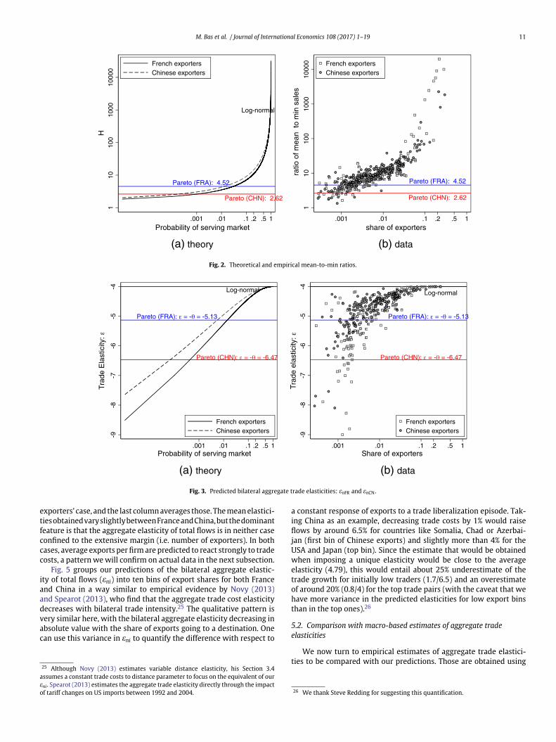
Panel (a) of Fig. 2 depicts the theoretical relationship between theratio of mean to minimum sales, H(a∗

ni) in Eqs. (8) and (9), and theprobability of serving the destination market, G(a∗

ni), spanning overvalues of the cutoff a∗

ni. Under Pareto heterogeneity, H is constant butthis property of scale invariance is specific to the Pareto: H is increas-ing in G under log-normal. Panel (b) of Fig. 2 depicts the empirical

22 We show in Appendix A that the values taken by a and l do not affect calculationsof the trade elasticity.

counterpart of this relationship as observed for French and Chineseexporters in 2000 for all countries in the world. On the x-axis isthe share of exporters serving each of those markets.23 Immediatelyapparent is the non-constant nature of the mean-to-min ratio in thedata, contradicting the Pareto prediction. This finding is very robustwhen considering alternatives to the minimum sales (which mightbe noisy because of statistical threshold effects) for the denomina-tor of H, that is different quantiles of the export distribution (resultsavailable upon request). In a further effort to minimize noise in thecalculation of the mean-to-min ratio, the figures are calculated foreach of the 99 HS2 product categories and averaged. In the rest of thesection, we will stick to this approach for the calculation of elasticities,done at the HS2 level before being averaged, which also simplifiesexposition (detailed sector-level results are provided in Section 6).

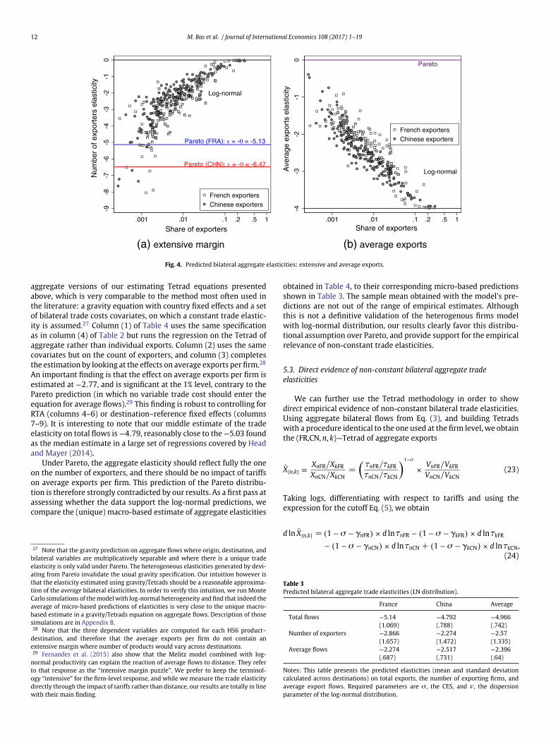
Fig. 3 turns to the predicted aggregate trade elasticities.24 Func-tional forms Eqs. (19) and (20) combined with Eq. (11), are used todeliver bilateral aggregate trade elasticity of total flows, eni, underthe two alternative distributional assumptions:

ePni = −h, and eLN

ni = 1 − s − 1m

h

(ln a∗

ni + l

m+ (s − 1)m

).

(22)

Parallel to Fig. 2, panel (a) of Fig. 3 shows the theoretical relationshipbetween those elasticities and G(a∗

ni), while panel (b) plots the sameelasticities evaluated for each individual destination country againstthe empirical counterpart of G(a∗

ni) (described in footnote 23). Again,the Pareto case has a constant prediction, while log-normal predictsa trade elasticity that is declining (in absolute value) with easinessof the market. Panel (b) confirms the large variance of trade elastici-ties according to the share of exporters that are active in each of themarkets. It also shows that the response of aggregate flows to tradecosts is reduced (in absolute value) when the market becomes easier.The intuition is that for very difficult markets, the individual reactionof incumbent firms is supplemented with entry of exporters selectedamong the most efficient firms. The latter effect becomes negligiblefor the easiest markets, yielding e to approach the firm-level tradeelasticity. This mechanism becomes very clear when looking at thepatterns of the extensive margin and average export elasticities inFig. 4.

The predicted elasticity on the extensive margin is also rising withmarket toughness as shown in panel (a) of Fig. 4. The inverse rela-tionship is true for average exports per firm (panel b). When a marketis very easy and most exporters make it there, the extensive marginelasticity goes to zero, and the response of average exports per firmgoes to the value of the firm-level trade elasticity, 1 −s , as shown inFig. 4 when the share of exporters increase. While this should intu-itively be true in general, Pareto does not allow for this change inelasticities across markets, since the response of average exports perfirm should be uniformly 0, while the total response is entirely dueto the (constant) extensive margin elasticity.

In Table 3, we compute the mean and standard deviation of thebilateraltradeelasticitiescalculatedusingthelog-normaldistribution,and presented in Figs. 3 and 4. The first column presents the statis-tics for the French exporters’ sample, the second one is the Chinese

23 On the x-axis we have the share of exporters serving each market n computedas the number of French and Chinese firms serving market n in 2000 conditionalon exporting (divided by the total number of exporters in each origin). The exactempirical counterpart of G(a∗

ni) would require to divide the number of actual Frenchand Chinese exporters to n by the set of potential exporters in France and China.We don’t observe that last number. However, the theoretical and the empiricalproportion of exporters differ only by a multiplicative constant, leaving the shape ofthe (logged) relationship unchanged.24 See Appendix A for details.

M. Bas et al. / Journal of International Economics 108 (2017) 1–19 11

Pareto (FRA): 4.52

Pareto (CHN): 2.62

Log-normal1

1010

010

0010

000

H

.001 .01 .1 .2 .5 1Probability of serving market

French exportersChinese exporters

Pareto (FRA): 4.52

Pareto (CHN): 2.62

110

100

1000

1000

0

ratio

of m

ean

to m

in s

ales

.001 .01 .1 .2 .5 1share of exporters

French exportersChinese exporters

(b) data(a) theory

Fig. 2. Theoretical and empirical mean-to-min ratios.

Pareto (FRA): = - = -5.13

Pareto (CHN): = - = -6.47

Log-normal

-9-8

-7-6

-5-4

Trad

e E

last

icity

:

.001 .01 .1 .2 .5 1Probability of serving market

French exportersChinese exporters

Pareto (FRA): = - = -5.13

Pareto (CHN): = - = -6.47

Log-normal-9

-8-7

-6-5

-4Tr

ade

elas

ticity

:

.001 .01 .1 .2 .5 1Share of exporters

French exportersChinese exporters

(b) data(a) theory

Fig. 3. Predicted bilateral aggregate trade elasticities: enFR and enCN.

exporters’ case, and the last column averages those. The mean elastici-tiesobtainedvaryslightlybetweenFranceandChina,butthedominantfeature is that the aggregate elasticity of total flows is in neither caseconfined to the extensive margin (i.e. number of exporters). In bothcases, average exports per firm are predicted to react strongly to tradecosts, a pattern we will confirm on actual data in the next subsection.

Fig. 5 groups our predictions of the bilateral aggregate elastic-ity of total flows (eni) into ten bins of export shares for both Franceand China in a way similar to empirical evidence by Novy (2013)and Spearot (2013), who find that the aggregate trade cost elasticitydecreases with bilateral trade intensity.25 The qualitative pattern isvery similar here, with the bilateral aggregate elasticity decreasing inabsolute value with the share of exports going to a destination. Onecan use this variance in eni to quantify the difference with respect to

25 Although Novy (2013) estimates variable distance elasticity, his Section 3.4assumes a constant trade costs to distance parameter to focus on the equivalent of oureni . Spearot (2013) estimates the aggregate trade elasticity directly through the impactof tariff changes on US imports between 1992 and 2004.

a constant response of exports to a trade liberalization episode. Tak-ing China as an example, decreasing trade costs by 1% would raiseflows by around 6.5% for countries like Somalia, Chad or Azerbai-jan (first bin of Chinese exports) and slightly more than 4% for theUSA and Japan (top bin). Since the estimate that would be obtainedwhen imposing a unique elasticity would be close to the averageelasticity (4.79), this would entail about 25% underestimate of thetrade growth for initially low traders (1.7/6.5) and an overestimateof around 20% (0.8/4) for the top trade pairs (with the caveat that wehave more variance in the predicted elasticities for low export binsthan in the top ones).26

5.2. Comparison with macro-based estimates of aggregate tradeelasticities

We now turn to empirical estimates of aggregate trade elastici-ties to be compared with our predictions. Those are obtained using

26 We thank Steve Redding for suggesting this quantification.

12 M. Bas et al. / Journal of International Economics 108 (2017) 1–19

Pareto (FRA): = - = -5.13

Pareto (CHN): = - = -6.47

Log-normal

-9-8

-7-6

-5-4

-3-2

-10

Num

ber

of e

xpor

ters

ela

stic

ity

.001 .01 .1 .2 .5 1

Share of exporters

French exportersChinese exporters

Pareto

Log-normal

-4-3

-2-1

0

Ave

rage

exp

orts

ela

stic

ity

.001 .01 .1 .2 .5 1Share of exporters

French exportersChinese exporters

(b) average exports(a) extensive margin

Fig. 4. Predicted bilateral aggregate elasticities: extensive and average exports.

aggregate versions of our estimating Tetrad equations presentedabove, which is very comparable to the method most often used inthe literature: a gravity equation with country fixed effects and a setof bilateral trade costs covariates, on which a constant trade elastic-ity is assumed.27 Column (1) of Table 4 uses the same specificationas in column (4) of Table 2 but runs the regression on the Tetrad ofaggregate rather than individual exports. Column (2) uses the samecovariates but on the count of exporters, and column (3) completesthe estimation by looking at the effects on average exports per firm.28

An important finding is that the effect on average exports per firm isestimated at −2.77, and is significant at the 1% level, contrary to thePareto prediction (in which no variable trade cost should enter theequation for average flows).29 This finding is robust to controlling forRTA (columns 4–6) or destination–reference fixed effects (columns7–9). It is interesting to note that our middle estimate of the tradeelasticity on total flows is −4.79, reasonably close to the −5.03 foundas the median estimate in a large set of regressions covered by Headand Mayer (2014).

Under Pareto, the aggregate elasticity should reflect fully the oneon the number of exporters, and there should be no impact of tariffson average exports per firm. This prediction of the Pareto distribu-tion is therefore strongly contradicted by our results. As a first pass atassessing whether the data support the log-normal predictions, wecompare the (unique) macro-based estimate of aggregate elasticities

27 Note that the gravity prediction on aggregate flows where origin, destination, andbilateral variables are multiplicatively separable and where there is a unique tradeelasticity is only valid under Pareto. The heterogeneous elasticities generated by devi-ating from Pareto invalidate the usual gravity specification. Our intuition however isthat the elasticity estimated using gravity/Tetrads should be a reasonable approxima-tion of the average bilateral elasticities. In order to verify this intuition, we run MonteCarlo simulations of the model with log-normal heterogeneity and find that indeed theaverage of micro-based predictions of elasticities is very close to the unique macro-based estimate in a gravity/Tetrads equation on aggregate flows. Description of thosesimulations are in Appendix B.28 Note that the three dependent variables are computed for each HS6 product–

destination, and therefore that the average exports per firm do not contain anextensive margin where number of products would vary across destinations.29 Fernandes et al. (2015) also show that the Melitz model combined with log-

normal productivity can explain the reaction of average flows to distance. They referto that response as the “intensive margin puzzle”. We prefer to keep the terminol-ogy “intensive” for the firm-level response, and while we measure the trade elasticitydirectly through the impact of tariffs rather than distance, our results are totally in linewith their main finding.

obtained in Table 4, to their corresponding micro-based predictionsshown in Table 3. The sample mean obtained with the model’s pre-dictions are not out of the range of empirical estimates. Althoughthis is not a definitive validation of the heterogenous firms modelwith log-normal distribution, our results clearly favor this distribu-tional assumption over Pareto, and provide support for the empiricalrelevance of non-constant trade elasticities.

5.3. Direct evidence of non-constant bilateral aggregate tradeelasticities

We can further use the Tetrad methodology in order to showdirect empirical evidence of non-constant bilateral trade elasticities.Using aggregate bilateral flows from Eq. (3), and building Tetradswith a procedure identical to the one used at the firm level, we obtainthe (FR,CN, n, k)—Tetrad of aggregate exports

X{n,k} ≡ XnFR/XkFR

XnCN/XkCN=

(tnFR/tkFR

tnCN/tkCN

)1−s

× VnFR/VkFR

VnCN/VkCN(23)

Taking logs, differentiating with respect to tariffs and using theexpression for the cutoff Eq. (5), we obtain

d ln X{n,k} = (1 − s − cnFR) × d ln tnFR − (1 − s − ckFR) × d ln tkFR

− (1 − s − cnCN) × d ln tnCN + (1 − s − ckCN) × d ln tkCN,(24)

Table 3Predicted bilateral aggregate trade elasticities (LN distribution).

France China Average

Total flows −5.14 −4.792 −4.966(1.069) (.788) (.742)

Number of exporters −2.866 −2.274 −2.57(1.657) (1.472) (1.335)

Average flows −2.274 −2.517 −2.396(.687) (.731) (.64)

Notes: This table presents the predicted elasticities (mean and standard deviationcalculated across destinations) on total exports, the number of exporting firms, andaverage export flows. Required parameters are s , the CES, and m, the dispersionparameter of the log-normal distribution.

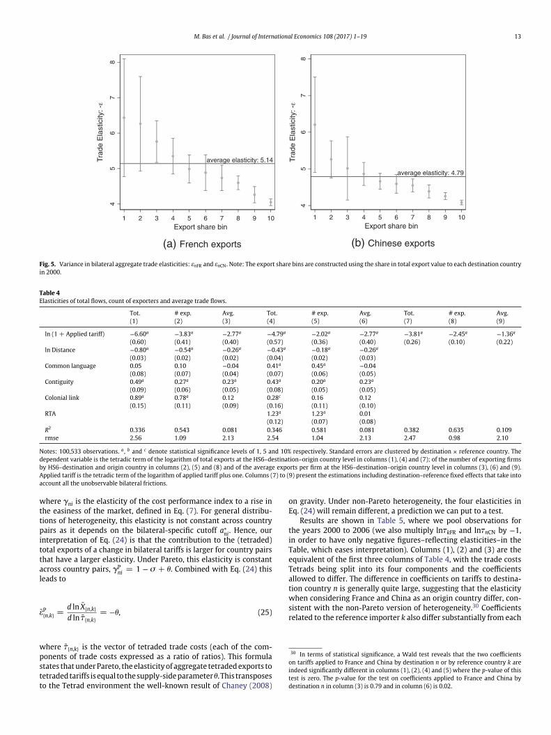
M. Bas et al. / Journal of International Economics 108 (2017) 1–19 13

average elasticity: 5.14

45

67

8

Trad

e E

last

icity

: -

1 2 3 4 5 6 7 8 9 10Export share bin

average elasticity: 4.79

45

67

8

Trad

e E

last

icity

: -

1 2 3 4 5 6 7 8 9 10Export share bin

(b) Chinese exports(a) French exports

Fig. 5. Variance in bilateral aggregate trade elasticities: enFR and enCN. Note: The export share bins are constructed using the share in total export value to each destination countryin 2000.

Table 4Elasticities of total flows, count of exporters and average trade flows.

Tot. # exp. Avg. Tot. # exp. Avg. Tot. # exp. Avg.(1) (2) (3) (4) (5) (6) (7) (8) (9)

ln (1 + Applied tariff) −6.60a −3.83a −2.77a −4.79a −2.02a −2.77a −3.81a −2.45a −1.36a

(0.60) (0.41) (0.40) (0.57) (0.36) (0.40) (0.26) (0.10) (0.22)ln Distance −0.80a −0.54a −0.26a −0.43a −0.18a −0.26a

(0.03) (0.02) (0.02) (0.04) (0.02) (0.03)Common language 0.05 0.10 −0.04 0.41a 0.45a −0.04

(0.08) (0.07) (0.04) (0.07) (0.06) (0.05)Contiguity 0.49a 0.27a 0.23a 0.43a 0.20a 0.23a

(0.09) (0.06) (0.05) (0.08) (0.05) (0.05)Colonial link 0.89a 0.78a 0.12 0.28c 0.16 0.12

(0.15) (0.11) (0.09) (0.16) (0.11) (0.10)RTA 1.23a 1.23a 0.01

(0.12) (0.07) (0.08)R2 0.336 0.543 0.081 0.346 0.581 0.081 0.382 0.635 0.109rmse 2.56 1.09 2.13 2.54 1.04 2.13 2.47 0.98 2.10

Notes: 100,533 observations. a , b and c denote statistical significance levels of 1, 5 and 10% respectively. Standard errors are clustered by destination × reference country. Thedependent variable is the tetradic term of the logarithm of total exports at the HS6–destination–origin country level in columns (1), (4) and (7); of the number of exporting firmsby HS6–destination and origin country in columns (2), (5) and (8) and of the average exports per firm at the HS6–destination–origin country level in columns (3), (6) and (9).Applied tariff is the tetradic term of the logarithm of applied tariff plus one. Columns (7) to (9) present the estimations including destination–reference fixed effects that take intoaccount all the unobservable bilateral frictions.

where cni is the elasticity of the cost performance index to a rise inthe easiness of the market, defined in Eq. (7). For general distribu-tions of heterogeneity, this elasticity is not constant across countrypairs as it depends on the bilateral-specific cutoff a∗

ni. Hence, ourinterpretation of Eq. (24) is that the contribution to the (tetraded)total exports of a change in bilateral tariffs is larger for country pairsthat have a larger elasticity. Under Pareto, this elasticity is constantacross country pairs, cP

ni = 1 − s + h. Combined with Eq. (24) thisleads to

eP{n,k} =

d ln X{n,k}d ln t{n,k}

= −h, (25)

where t{n,k} is the vector of tetraded trade costs (each of the com-ponents of trade costs expressed as a ratio of ratios). This formulastates that under Pareto, the elasticity of aggregate tetraded exports totetraded tariffs is equal to the supply-side parameterh. This transposesto the Tetrad environment the well-known result of Chaney (2008)

on gravity. Under non-Pareto heterogeneity, the four elasticities inEq. (24) will remain different, a prediction we can put to a test.

Results are shown in Table 5, where we pool observations forthe years 2000 to 2006 (we also multiply lntkFR and lntnCN by −1,in order to have only negative figures–reflecting elasticities–in theTable, which eases interpretation). Columns (1), (2) and (3) are theequivalent of the first three columns of Table 4, with the trade costsTetrads being split into its four components and the coefficientsallowed to differ. The difference in coefficients on tariffs to destina-tion country n is generally quite large, suggesting that the elasticitywhen considering France and China as an origin country differ, con-sistent with the non-Pareto version of heterogeneity.30 Coefficientsrelated to the reference importer k also differ substantially from each

30 In terms of statistical significance, a Wald test reveals that the two coefficientson tariffs applied to France and China by destination n or by reference country k areindeed significantly different in columns (1), (2), (4) and (5) where the p-value of thistest is zero. The p-value for the test on coefficients applied to France and China bydestination n in column (3) is 0.79 and in column (6) is 0.02.

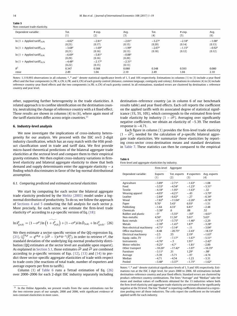
14 M. Bas et al. / Journal of International Economics 108 (2017) 1–19

Table 5Non-constant trade elasticity.

Dependent variable: Tot. # exp. Avg. Tot. # exp. Avg.(1) (2) (3) (4) (5) (6)

ln (1 + Applied tariff)n,FR −4.82a −2.81a −2.01a −3.27a −2.18a −1.08a

(0.23) (0.17) (0.15) (0.20) (0.14) (0.13)ln (1 + Applied tariff)n,CN −3.68a −1.69a −1.99a −2.07a −1.15a −0.92a

(0.21) (0.16) (0.13) (0.18) (0.12) (0.12)ln (1 + Applied tariff)k,FR −6.69a −5.81a −0.88a

(0.29) (0.16) (0.20)ln (1 + Applied tariff)k,CN −4.48a −2.17a −2.31a

(0.22) (0.15) (0.13)R2 0.347 0.588 0.080 0.348 0.593 0.080rmse 2.49 1.04 2.10 2.49 1.04 2.10

Notes: 1,119,993 observations in all columns. a , b and c denote statistical significance levels of 1, 5 and 10% respectively. Estimations in columns (1) to (3) include a year fixedeffect and the four components (n, FR; n, CN; k, FR; and k, CN) of each gravity control (distance, common language, contiguity and colony). Estimations in columns (4) to (6) includereference country–year fixed effects and the two components (n, FR; n, CN) of each gravity control. In all estimations, standard errors are clustered by destination × referencecountry and year level.

other, supporting further heterogeneity in the trade elasticities. Arelated approach is to confine identification on the destination coun-try, neutralizing the change of reference country with a k fixed effect.Those results are shown in columns (4) to (6), where again most ofthe tariff elasticities differ across origin countries.31

6. Industry-level analysis

We now investigate the implications of cross-industry hetero-geneity for our analysis. We proceed with the ISIC rev3 2-digitindustry classification, which has an easy match with the HS6 prod-uct classification used in trade and tariff data. We first providemicro-based theoretical predictions of the bilateral aggregate tradeelasticities at the sectoral level and compare them to their empiricalgravity estimates. We then exploit cross-industry variations in firm-level elasticity and bilateral aggregate elasticity to show that bothdemand and supply determinants enter the aggregate elasticity — afinding which discriminates in favor of the log-normal distributionalassumption.

6.1. Comparing predicted and estimated sectoral elasticities

We start by computing for each sector the bilateral aggregatetrade elasticity predicted by the Melitz (2003) model under a log-normal distribution of productivity. To do so, we follow the approachof Sections 4 and 5 conducting the full analysis for each sector p.More precisely, for each sector, we estimate the firm-level tradeelasticity sp according to a p-specific version of Eq. (18):

ln xp{j,n,k} = (1 −sp) ln

˜(1 + tp

{n,k})

+ (1 −sp)d ln D{n,k} + ln 4p{j,n,k}. (26)

We then estimate a sector-specific version of the QQ-regression Eq.(21), QLN,p

f = qLN,p + (sp − 1)mpV−1(Fpf ), in order to retrieve mp, the

standard deviation of the underlying log-normal productivity distri-bution (QQ estimates at the sector level are available upon request).As explained in Section 5.1, those estimates sp and mp are combinedaccording to p-specific versions of Eqs. (12), (13) and (14) to pre-dict three sector-specific aggregate elasticities of trade with respectto trade costs (the reactions of total trade, number of exporters andaverage exports per firm to tariffs).

Column (1) of Table 6 runs a Tetrad estimation of Eq. (26)over 2000–2006 for each 2-digit ISIC industry separately including

31 In the Online Appendix, we present results from the same estimations run forthe two extreme years of our sample, 2000 and 2006, with significant evidence ofnon-constant elasticities in most cases.

destination–reference country (as in column 6 of our benchmarkresults table) and year fixed effects. Each cell reports the coefficienton the applied tariffs with its associated degree of statistical signif-icance (1%, 5%, 10%), which corresponds to the estimated firm-leveltrade elasticity by industry (1 − sp). Averaging over significantlynegative coefficients, we obtain an elasticity of −5.39. The medianresponse is −4.71.

Each figure in column (1) provides the firm-level trade elasticity(1 − sp), needed for the calculation of p-specific bilateral aggre-gate trade elasticities. We summarize those elasticities by report-ing cross-sector cross-destination means and standard deviationsin Table 7. These statistics can then be compared to the empirical

Table 6Firm-level and aggregate elasticities by industry.

Firm-level Aggregate

Dependent variable: Exports Tot. exports # exporters Avg. exports(1) (2) (3) (4)

Agriculture −3.89a −2.71a −1.63a −1.08Food −3.53a −4.54a −1.23a −3.31a

Textile −4.18a −1.95a −1.63a −.32Wearing apparel −4.03a −4.21a −.43 −3.79a

Leather −2.84a −6.62a −.27 −6.34a

Wood −7.82b −11.04a −2.26a −8.78a

Paper 9.76a 5.43c 6.93a −1.51Publishing −1.64 4.33c 6.81a −2.48Chemicals −3.38a .6 .08 .52Rubber and plastic −5a −5.55a −.93b −4.61a

Non-metallic 4.56a 11.24a 5.61a 5.63a

Basic metals −4.73b −3.75b −1.46a −2.29Metals −2.39b −1.41b 1.87a −3.28a

Non-electrical machinery −4.71a −3.14a −.11 −3.04a

Office machinery −8.48 −20.75a −2.43c −18.33a

Electrical machinery −2.5 .55 2.19a −1.63b

Equip. radio, TV −7.5a −7.17a −1.67a −5.51a

Instruments −4.76a −.5 1.91a −2.42a

Motor vehicles −9.25a −4.7c −1.81c −2.89Other transport −10.26a −17.42a −1.07c −16.35a

Furniture −3.11a .31 1.29a −.98c

Average −5.39 −5.71 −.97 −4.74Median −4.71 −4.54 −1.23 −3.31Pooled −3.48a −3.37a −1.75a −1.62a

Notes: a , b and c denote statistical significance levels of 1, 5 and 10% respectively. Esti-mations run at the ISIC 2 digit level, for years 2000 to 2006. All estimations includedestination–reference country and year fixed effects. Standard errors are clustered byproduct–reference country combinations. The lines “Average” and “Median” take themean and median values of coefficients obtained for the 13 industries where boththe firm-level elasticity and aggregate trade elasticity are estimated to be significantlynegative at the 5% level. The line “Pooled” is reporting coefficients obtained in a regres-sion pooling over all those industries. The cells report the coefficient on the tetradedapplied tariffs for each industry.

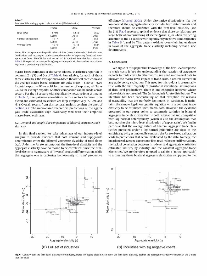
M. Bas et al. / Journal of International Economics 108 (2017) 1–19 15

Table 7Predicted bilateral aggregate trade elasticities (LN distribution).

France China Average

Total flows −5.492 −5.513 −5.502(.369) (.451) (.308)

Number of exporters −1.117 −.8 −.958(.788) (.971) (.762)

Average flows −4.375 −4.713 −4.544(.608) (.66) (.564)

Notes: This table presents the predicted elasticities (mean and standard deviation overdestinations and sectors) on total exports, the number of exporting firms, and aver-age export flows. The CES for each sector, sp , is obtained from the first column ofTable 6. Unreported sector-specific QQ-regressions yield mp , the standard deviation oflog-normal productivity distribution.

macro-based estimates of the same bilateral elasticities reported incolumns (2), (3) and (4) of Table 6. Remarkably, for each of thosethree elasticities, the average micro-based theoretical prediction andthe average macro-based estimate are quite close: −5.50 vs −6.04for total export, −.96 vs −.97 for the number of exporter, −4.54 vs−4.74 for average exports. Another comparison can be made acrosssectors. For the 13 sectors with significantly negative joint estimatesin Table 6, the pairwise correlations across sectors between pre-dicted and estimated elasticities are large (respectively .77, .59, and.61). Overall, results from this sectoral analysis confirm the ones ofSection 5.2: The micro-based theoretical predictions of the aggre-gate trade elasticities align reasonably well with their empiricalmacro-based estimates.

6.2. Demand and supply side components of bilateral aggregate tradeelasticity

In this final section, we take advantage of our industry-levelanalysis to provide evidence that both demand and supply-sidedeterminants enter the bilateral aggregate elasticity of total flows(eni). Under the Pareto assumption, the firm-level elasticity and theaggregate elasticity have no reason to be correlated, since the firm-level elasticity is a measure of (inverse) product differentiation, whilethe aggregate one is capturing homogeneity in firms’ productive

efficiency (Chaney, 2008). Under alternative distributions like thelog-normal, the aggregate elasticity includes both determinants andtherefore should be correlated with the firm-level elasticity (seeEq. (1)). Fig. 6 reports graphical evidence that those correlations arelarge, both when considering all sectors (panel a), or when restrictingattention to the 13 sectors with significantly negative joint estimatesin Table 6 (panel b). This pattern exhibits overwhelming evidencein favor of the aggregate trade elasticity including demand sidedeterminants.

7. Conclusion

We argue in this paper that knowledge of the firm-level responseto trade costs is key for understanding the reaction of aggregateexports to trade costs. In other words, we need micro-level data touncover the macro-level impact of trade costs, a central element inany trade policy evaluation. This need for micro-data is presumablytrue with the vast majority of possible distributional assumptionsof firm-level productivity. There is one exception however wheremicro-data is not needed: The (unbounded) Pareto distribution. Theliterature has been concentrating on that exception for reasonsof tractability that are perfectly legitimate. In particular, it main-tains the simple log-linear gravity equation with a constant tradeelasticity to be estimated with macro-data. However, the evidencepresented in our paper points to systematic variation in bilateralaggregate trade elasticities that is both substantial and compatiblewith log-normal heterogeneity (which is also the assumption thatbest matches the micro-level distribution of export sales). We find inparticular that the average values of bilateral aggregate trade elas-ticities predicted under a log-normal calibration are close to theempirical gravity estimates. By contrast, the Pareto-based calibrationleads to predictions that seem invalidated by the data. Namely, theinvariance of average exports per firm to ad-valorem tariff variations,the lack of correlation between firm-level and aggregate elasticitiesestimated industry by industry, and the constant aggregate tradeelasticities. We are therefore tempted to call for a “micro-approach”to estimating those bilateral aggregate elasticities as opposed to the

AgricultureFoodTextileWearing apparel

Leather

Wood

Paper

Publishing

Chemicals

Rubber and plastic

Non-metallic

Basic metals

Metals

Non electrical machinery

Electrical machinery

Equip. Radio, TV

Instruments

Motor Vehicles

Other Transport

Furniture

-15

-10

-50

510

Mic

ro e

last

icity

(1-

)

-30 -20 -10 0 10Aggregate elasticity ( )

AgricultureFood

TextileWearing apparel

Leather

Wood

Rubber and plasticBasic metals

Metals

Non electrical machinery

Equip. Radio, TV

Motor Vehicles

Other Transport

-15

-10

-50

Mic

ro e

last

icity

(1-

)

-20 -15 -10 -5 0Aggregate elasticity ( )

(a) Full set of industries (b) Industries with sig.negative coeffs.

Fig. 6. Country-pair and firm-level elasticities by industry. Note: The figure plots in each panel the firm-level elasticity against the aggregate elasticity estimated at the 2-digitindustry level.

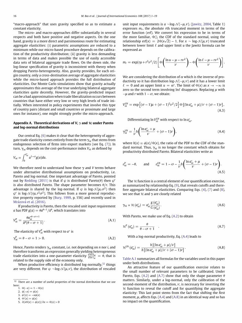
16 M. Bas et al. / Journal of International Economics 108 (2017) 1–19

“macro-approach” that uses gravity specified so as to estimate aconstant elasticity.

The micro- and macro-approaches differ substantially in severalrespects and both have positive and negative aspects. On the onehand, gravity is a more direct and parsimonious route for estimatingaggregate elasticities: (i) parametric assumptions are reduced to aminimum while our micro-based procedure depends on the calibra-tion of the productivity distribution; (ii) gravity is less demandingin terms of data and makes possible the use of easily accessibledata sets of bilateral aggregate trade flows. On the down side, thelog-linear specification of gravity is inconsistent with theory whendropping Pareto-heterogeneity. Also, gravity provides, for each ori-gin country, only a cross-destination average of aggregate elasticitieswhile the micro-based approach provides the full distribution ofelasticities. Our Monte Carlo simulations show that gravity actuallyapproximates this average of the true underlying bilateral aggregateelasticities quite decently. However, the gravity-predicted impactcan be a bad approximation when trade liberalization occurs betweencountries that have either very low or very high levels of trade ini-tially. When interested in policy experiments that involve this typeof country pairs (distant and small countries or proximate and largeones for instance), one might strongly prefer the micro-approach.

Appendix A. Theoretical derivations of V, c and H under Paretoand log-normal distributions

Our central Eq. (6) makes it clear that the heterogeneity of aggre-gate trade elasticity comes entirely from the term cni that stems fromendogenous selection of firms into export markets (see Eq. (7)). Inturn, cni depends on the cost-performance index Vni as defined by

Vni ≡∫ a∗

ni

0a1−sg(a)da.

We therefore need to understand how these c and V terms behaveunder alternative distributional assumptions on productivity, i.e.Pareto and log-normal. One important advantage of Pareto, pointedout by Redding (2011) is that if v is distributed Pareto(h) then vr

is also distributed Pareto. The shape parameter becomes h/r. Thisadvantage is shared by the log-normal. If v is log-N (l,s2) thenvr is log-N (rl, r2s2). This follows from a more general reproduc-tive property reported by (Bury, 1999, p. 156) and recently used inMrázová et al. (2016).

If productivity is Pareto, then the rescaled unit input requirementa has PDF g(a) = hah−1/ah, which translates into

VPni =

ha∗h−s+1ni

ah(h − s + 1). (A.1)

The elasticity of VPni with respect to a∗ is

cPni = h − s + 1 > 0. (A.2)

Hence, Pareto renders cni constant, i.e. not depending on n nor i, andtherefore transforms an expression generally yielding heterogeneoustrade elasticities into a one-parameter elasticity d ln Xni

d ln tni= h, that is

related to the supply side of the economy only.When productive efficiency is distributed log-normally,32 things

are very different. For v ∼log-N (l,m), the distribution of rescaled

32 There are a number of useful properties of the normal distribution that we usehere:

1. V(−x) = 1 − V(x)2. 0(−x) = 0(x)3. 0′(x) = −x0(x)4. V′(x) = 0(x)5. ∂(xV(x) + 0(x))/∂x = V(x) > 0

unit input requirements is a ∼log-N (−l,m). (Jawitz, 2004, Table 1)expresses mr, the absolute rth truncated moment in terms of theerror function (erf). We convert his expression to be in terms ofthe more familiar, V(), the CDF of the standard normal, using therelationship erf(x) = 2V(x

√2) − 1. For x ∼ log-N (l,m) truncated

between lower limit � and upper limit u the Jawitz formula can beexpressed as

mr = exp(rl+r2m2/2)

[V

(ln u − l − rm2

m

)− V

(ln � − l − rm2

m

)].

We are considering the distribution of a which is the inverse of pro-ductivity so it has distribution log-N (−l,m) and it has a lower limit� = 0 and an upper limit u = a∗. The limit of V(x) as x → −∞ iszero so the second term involving ln� disappears. Replacing l with−l and r with 1 − s , we obtain:

VLNni = exp

[(s − 1)l + (s − 1)2m2/2

]V

[(ln a∗

ni + l)/m + (s − 1)m]

,

(A.3)

Differentiating ln VLNni with respect to ln a∗

ni,

cLNni =

1m

h

(ln a∗

ni + l

m+ (s − 1)m

), (A.4)

where h(x) ≡ 0(x)/V(x), the ratio of the PDF to the CDF of the stan-dard normal. Thus, cni is no longer the constant which obtains forproductivity distributed Pareto. Bilateral elasticities write as

ePni = −h, and eLN

ni = 1 − s − 1m

h

(ln a∗

ni + l

m+ (s − 1)m

).

(A.5)

The H function is a central element of our quantification exercise,as summarized by relationship Eq. (9), that reveals cutoffs and there-fore aggregate bilateral elasticities. Comparing Eqs. (4), (7) and (8),we see that H and c are closely related

cni × H(a∗

ni

)= a∗

ni

g(a∗

ni

)G

(a∗

ni

) . (A.6)

With Pareto, we make use of Eq. (A.2) to obtain

HP (a∗

ni

)=

h

h − s + 1. (A.7)

With a log-normal productivity, Eq. (A.4) leads to

HLN (a∗

ni

)=

h[(ln a∗

ni + l)/m]

h[(ln a∗

ni + l)/m + (s − 1)m] . (A.8)

Table A.1 summarizes all formulas for the variables used in this paperunder both distributions.

An attractive feature of our quantification exercise relates tothe small number of relevant parameters to be calibrated. UnderPareto, Eqs. (A.2) and (A.7) show that only the shape parameter h

matters. Similarly, under a log-normal, only the calibration of thesecond-moment of the distribution, m, is necessary for inverting theH function to reveal the cutoff and for quantifying the aggregateelasticity: This last point stems from the fact that shifting the firstmoment, l, affects Eqs. (A.4) and (A.8) in an identical way and so hasno impact on the quantification.

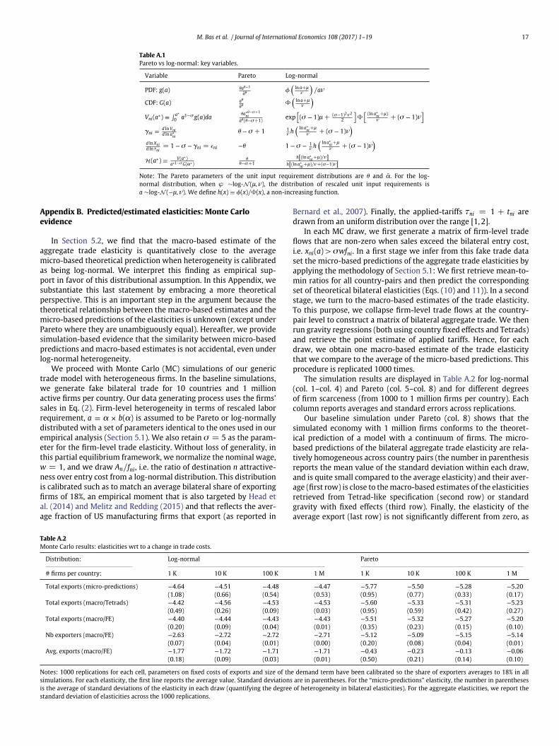
M. Bas et al. / Journal of International Economics 108 (2017) 1–19 17

Table A.1Pareto vs log-normal: key variables.

Variable Pareto Log-normal

PDF: g(a) hah−1

ah0

(ln a+l

m

)/am

CDF: G(a) ah

ahV

(ln a+l

m

)Vni(a∗) ≡ ∫ a∗

0 a1−sg(a)daha∗h−s+1

niah(h−s+1)

exp[(s − 1)l + (s−1)2m2

2

]V

[ (ln a∗ni+l)m + (s − 1)m

]cni ≡ d ln Vni

d ln a∗ni

h − s + 1 1m h

( ln a∗ni+l

m + (s − 1)m)

d ln Xnid ln tni

= 1 − s − cni = 4ni −h 1 − s − 1m h

( ln a∗ni+l

m + (s − 1)m)

H(a∗) ≡ V(a∗)a∗1−s G(a∗)

hh−s+1

h[(ln a∗ni+l)/m]

h[(ln a∗ni+l)/m+(s−1)m]

Note: The Pareto parameters of the unit input requirement distributions are h and a. For the log-normal distribution, when v ∼log-N (l,m), the distribution of rescaled unit input requirements isa ∼log-N (−l,m). We define h(x) ≡ 0(x)/V(x), a non-increasing function.

Appendix B. Predicted/estimated elasticities: Monte Carloevidence

In Section 5.2, we find that the macro-based estimate of theaggregate trade elasticity is quantitatively close to the averagemicro-based theoretical prediction when heterogeneity is calibratedas being log-normal. We interpret this finding as empirical sup-port in favor of this distributional assumption. In this Appendix, wesubstantiate this last statement by embracing a more theoreticalperspective. This is an important step in the argument because thetheoretical relationship between the macro-based estimates and themicro-based predictions of the elasticities is unknown (except underPareto where they are unambiguously equal). Hereafter, we providesimulation-based evidence that the similarity between micro-basedpredictions and macro-based estimates is not accidental, even underlog-normal heterogeneity.

We proceed with Monte Carlo (MC) simulations of our generictrade model with heterogeneous firms. In the baseline simulations,we generate fake bilateral trade for 10 countries and 1 millionactive firms per country. Our data generating process uses the firms’sales in Eq. (2). Firm-level heterogeneity in terms of rescaled laborrequirement, a ≡ a × b(a) is assumed to be Pareto or log-normallydistributed with a set of parameters identical to the ones used in ourempirical analysis (Section 5.1). We also retain s = 5 as the param-eter for the firm-level trade elasticity. Without loss of generality, inthis partial equilibrium framework, we normalize the nominal wage,w = 1, and we draw An/fni, i.e. the ratio of destination n attractive-ness over entry cost from a log-normal distribution. This distributionis calibrated such as to match an average bilateral share of exportingfirms of 18%, an empirical moment that is also targeted by Head etal. (2014) and Melitz and Redding (2015) and that reflects the aver-age fraction of US manufacturing firms that export (as reported in

Bernard et al., 2007). Finally, the applied-tariffs tni = 1 + tni aredrawn from an uniform distribution over the range [1, 2].

In each MC draw, we first generate a matrix of firm-level tradeflows that are non-zero when sales exceed the bilateral entry cost,i.e. xni(a) >swfni. In a first stage we infer from this fake trade dataset the micro-based predictions of the aggregate trade elasticities byapplying the methodology of Section 5.1: We first retrieve mean-to-min ratios for all country-pairs and then predict the correspondingset of theoretical bilateral elasticities (Eqs. (10) and 11)). In a secondstage, we turn to the macro-based estimates of the trade elasticity.To this purpose, we collapse firm-level trade flows at the country-pair level to construct a matrix of bilateral aggregate trade. We thenrun gravity regressions (both using country fixed effects and Tetrads)and retrieve the point estimate of applied tariffs. Hence, for eachdraw, we obtain one macro-based estimate of the trade elasticitythat we compare to the average of the micro-based predictions. Thisprocedure is replicated 1000 times.

The simulation results are displayed in Table A.2 for log-normal(col. 1–col. 4) and Pareto (col. 5–col. 8) and for different degreesof firm scarceness (from 1000 to 1 million firms per country). Eachcolumn reports averages and standard errors across replications.

Our baseline simulation under Pareto (col. 8) shows that thesimulated economy with 1 million firms conforms to the theoret-ical prediction of a model with a continuum of firms. The micro-based predictions of the bilateral aggregate trade elasticity are rela-tively homogeneous across country pairs (the number in parenthesisreports the mean value of the standard deviation within each draw,and is quite small compared to the average elasticity) and their aver-age (first row) is close to the macro-based estimates of the elasticitiesretrieved from Tetrad-like specification (second row) or standardgravity with fixed effects (third row). Finally, the elasticity of theaverage export (last row) is not significantly different from zero, as

Table A.2Monte Carlo results: elasticities wrt to a change in trade costs.

Distribution: Log-normal Pareto

# firms per country: 1 K 10 K 100 K 1 M 1 K 10 K 100 K 1 M

Total exports (micro-predictions) −4.64 −4.51 −4.48 −4.47 −5.77 −5.50 −5.28 −5.20(1.08) (0.66) (0.54) (0.53) (0.95) (0.77) (0.33) (0.17)

Total exports (macro/Tetrads) −4.42 −4.56 −4.53 −4.53 −5.60 −5.33 −5.31 −5.23(0.49) (0.26) (0.09) (0.03) (0.95) (0.59) (0.42) (0.27)

Total exports (macro/FE) −4.40 −4.44 −4.43 −4.43 −5.51 −5.32 −5.27 −5.20(0.20) (0.09) (0.04) (0.01) (0.35) (0.23) (0.15) (0.10)

Nb exporters (macro/FE) −2.63 −2.72 −2.72 −2.71 −5.12 −5.09 −5.15 −5.14(0.07) (0.04) (0.01) (0.00) (0.20) (0.08) (0.04) (0.01)

Avg. exports (macro/FE) −1.77 −1.72 −1.71 −1.71 −0.43 −0.23 −0.13 −0.06(0.18) (0.09) (0.03) (0.01) (0.50) (0.21) (0.14) (0.10)

Notes: 1000 replications for each cell, parameters on fixed costs of exports and size of the demand term have been calibrated so the share of exporters averages to 18% in allsimulations. For each elasticity, the first line reports the average value. Standard deviations are in parentheses. For the “micro-predictions” elasticity, the number in parenthesesis the average of standard deviations of the elasticity in each draw (quantifying the degree of heterogeneity in bilateral elasticities). For the aggregate elasticities, we report thestandard deviation of elasticities across the 1000 replications.

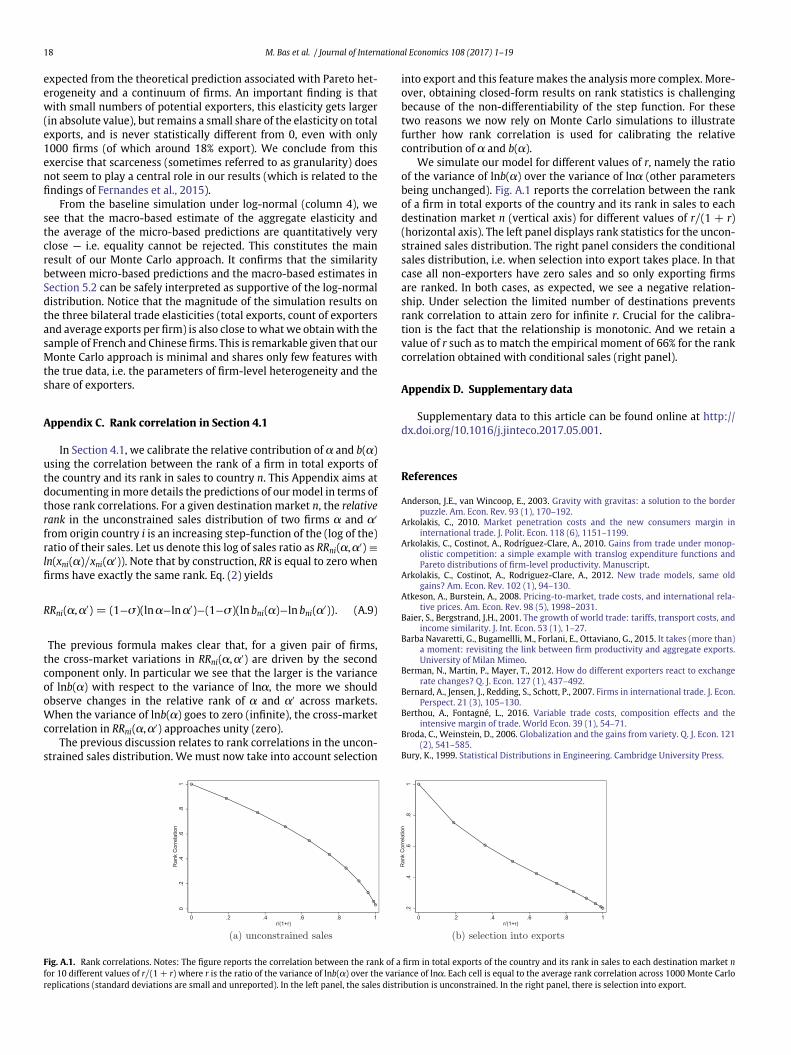
18 M. Bas et al. / Journal of International Economics 108 (2017) 1–19

expected from the theoretical prediction associated with Pareto het-erogeneity and a continuum of firms. An important finding is thatwith small numbers of potential exporters, this elasticity gets larger(in absolute value), but remains a small share of the elasticity on totalexports, and is never statistically different from 0, even with only1000 firms (of which around 18% export). We conclude from thisexercise that scarceness (sometimes referred to as granularity) doesnot seem to play a central role in our results (which is related to thefindings of Fernandes et al., 2015).

From the baseline simulation under log-normal (column 4), wesee that the macro-based estimate of the aggregate elasticity andthe average of the micro-based predictions are quantitatively veryclose — i.e. equality cannot be rejected. This constitutes the mainresult of our Monte Carlo approach. It confirms that the similaritybetween micro-based predictions and the macro-based estimates inSection 5.2 can be safely interpreted as supportive of the log-normaldistribution. Notice that the magnitude of the simulation results onthe three bilateral trade elasticities (total exports, count of exportersand average exports per firm) is also close to what we obtain with thesample of French and Chinese firms. This is remarkable given that ourMonte Carlo approach is minimal and shares only few features withthe true data, i.e. the parameters of firm-level heterogeneity and theshare of exporters.

Appendix C. Rank correlation in Section 4.1

In Section 4.1, we calibrate the relative contribution of a and b(a)using the correlation between the rank of a firm in total exports ofthe country and its rank in sales to country n. This Appendix aims atdocumenting in more details the predictions of our model in terms ofthose rank correlations. For a given destination market n, the relativerank in the unconstrained sales distribution of two firms a and a′from origin country i is an increasing step-function of the (log of the)ratio of their sales. Let us denote this log of sales ratio as RRni(a,a′) ≡ln(xni(a)/xni(a′)). Note that by construction, RR is equal to zero whenfirms have exactly the same rank. Eq. (2) yields

RRni(a,a′) = (1−s)(lna−lna′)−(1−s)(ln bni(a)−ln bni(a′)). (A.9)

The previous formula makes clear that, for a given pair of firms,the cross-market variations in RRni(a,a′) are driven by the secondcomponent only. In particular we see that the larger is the varianceof lnb(a) with respect to the variance of lna, the more we shouldobserve changes in the relative rank of a and a′ across markets.When the variance of lnb(a) goes to zero (infinite), the cross-marketcorrelation in RRni(a,a′) approaches unity (zero).

The previous discussion relates to rank correlations in the uncon-strained sales distribution. We must now take into account selection

into export and this feature makes the analysis more complex. More-over, obtaining closed-form results on rank statistics is challengingbecause of the non-differentiability of the step function. For thesetwo reasons we now rely on Monte Carlo simulations to illustratefurther how rank correlation is used for calibrating the relativecontribution of a and b(a).

We simulate our model for different values of r, namely the ratioof the variance of lnb(a) over the variance of lna (other parametersbeing unchanged). Fig. A.1 reports the correlation between the rankof a firm in total exports of the country and its rank in sales to eachdestination market n (vertical axis) for different values of r/(1 + r)(horizontal axis). The left panel displays rank statistics for the uncon-strained sales distribution. The right panel considers the conditionalsales distribution, i.e. when selection into export takes place. In thatcase all non-exporters have zero sales and so only exporting firmsare ranked. In both cases, as expected, we see a negative relation-ship. Under selection the limited number of destinations preventsrank correlation to attain zero for infinite r. Crucial for the calibra-tion is the fact that the relationship is monotonic. And we retain avalue of r such as to match the empirical moment of 66% for the rankcorrelation obtained with conditional sales (right panel).

Appendix D. Supplementary data

Supplementary data to this article can be found online at http://dx.doi.org/10.1016/j.jinteco.2017.05.001.

References

Anderson, J.E., van Wincoop, E., 2003. Gravity with gravitas: a solution to the borderpuzzle. Am. Econ. Rev. 93 (1), 170–192.

Arkolakis, C., 2010. Market penetration costs and the new consumers margin ininternational trade. J. Polit. Econ. 118 (6), 1151–1199.

Arkolakis, C., Costinot, A., Rodríguez-Clare, A., 2010. Gains from trade under monop-olistic competition: a simple example with translog expenditure functions andPareto distributions of firm-level productivity. Manuscript.

Arkolakis, C., Costinot, A., Rodriguez-Clare, A., 2012. New trade models, same oldgains? Am. Econ. Rev. 102 (1), 94–130.

Atkeson, A., Burstein, A., 2008. Pricing-to-market, trade costs, and international rela-tive prices. Am. Econ. Rev. 98 (5), 1998–2031.

Baier, S., Bergstrand, J.H., 2001. The growth of world trade: tariffs, transport costs, andincome similarity. J. Int. Econ. 53 (1), 1–27.

Barba Navaretti, G., Bugamellli, M., Forlani, E., Ottaviano, G., 2015. It takes (more than)a moment: revisiting the link between firm productivity and aggregate exports.University of Milan Mimeo.

Berman, N., Martin, P., Mayer, T., 2012. How do different exporters react to exchangerate changes? Q. J. Econ. 127 (1), 437–492.

Bernard, A., Jensen, J., Redding, S., Schott, P., 2007. Firms in international trade. J. Econ.Perspect. 21 (3), 105–130.

Berthou, A., Fontagné, L., 2016. Variable trade costs, composition effects and theintensive margin of trade. World Econ. 39 (1), 54–71.

Broda, C., Weinstein, D., 2006. Globalization and the gains from variety. Q. J. Econ. 121(2), 541–585.

Bury, K., 1999. Statistical Distributions in Engineering. Cambridge University Press.

Fig. A.1. Rank correlations. Notes: The figure reports the correlation between the rank of a firm in total exports of the country and its rank in sales to each destination market nfor 10 different values of r/(1 + r) where r is the ratio of the variance of lnb(a) over the variance of lna. Each cell is equal to the average rank correlation across 1000 Monte Carloreplications (standard deviations are small and unreported). In the left panel, the sales distribution is unconstrained. In the right panel, there is selection into export.

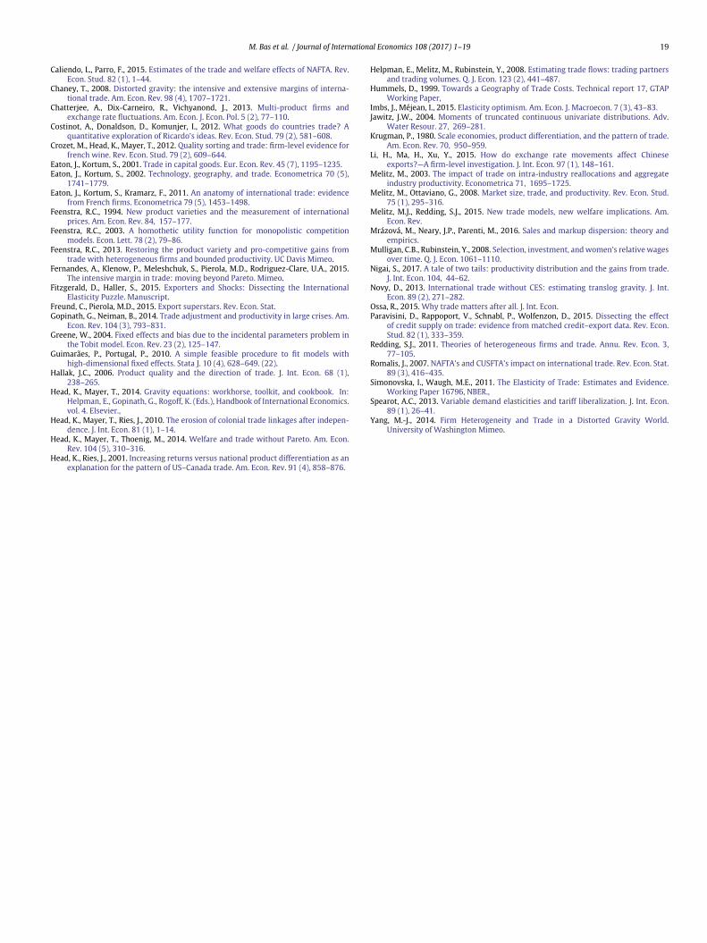
M. Bas et al. / Journal of International Economics 108 (2017) 1–19 19

Caliendo, L., Parro, F., 2015. Estimates of the trade and welfare effects of NAFTA. Rev.Econ. Stud. 82 (1), 1–44.

Chaney, T., 2008. Distorted gravity: the intensive and extensive margins of interna-tional trade. Am. Econ. Rev. 98 (4), 1707–1721.

Chatterjee, A., Dix-Carneiro, R., Vichyanond, J., 2013. Multi-product firms andexchange rate fluctuations. Am. Econ. J. Econ. Pol. 5 (2), 77–110.

Costinot, A., Donaldson, D., Komunjer, I., 2012. What goods do countries trade? Aquantitative exploration of Ricardo’s ideas. Rev. Econ. Stud. 79 (2), 581–608.

Crozet, M., Head, K., Mayer, T., 2012. Quality sorting and trade: firm-level evidence forfrench wine. Rev. Econ. Stud. 79 (2), 609–644.

Eaton, J., Kortum, S., 2001. Trade in capital goods. Eur. Econ. Rev. 45 (7), 1195–1235.Eaton, J., Kortum, S., 2002. Technology, geography, and trade. Econometrica 70 (5),

1741–1779.Eaton, J., Kortum, S., Kramarz, F., 2011. An anatomy of international trade: evidence

from French firms. Econometrica 79 (5), 1453–1498.Feenstra, R.C., 1994. New product varieties and the measurement of international

prices. Am. Econ. Rev. 84, 157–177.Feenstra, R.C., 2003. A homothetic utility function for monopolistic competition

models. Econ. Lett. 78 (2), 79–86.Feenstra, R.C., 2013. Restoring the product variety and pro-competitive gains from

trade with heterogeneous firms and bounded productivity. UC Davis Mimeo.Fernandes, A., Klenow, P., Meleshchuk, S., Pierola, M.D., Rodriguez-Clare, U.A., 2015.

The intensive margin in trade: moving beyond Pareto. Mimeo.Fitzgerald, D., Haller, S., 2015. Exporters and Shocks: Dissecting the International

Elasticity Puzzle. Manuscript.Freund, C., Pierola, M.D., 2015. Export superstars. Rev. Econ. Stat.Gopinath, G., Neiman, B., 2014. Trade adjustment and productivity in large crises. Am.

Econ. Rev. 104 (3), 793–831.Greene, W., 2004. Fixed effects and bias due to the incidental parameters problem in

the Tobit model. Econ. Rev. 23 (2), 125–147.Guimarães, P., Portugal, P., 2010. A simple feasible procedure to fit models with

high-dimensional fixed effects. Stata J. 10 (4), 628–649. (22).Hallak, J.C., 2006. Product quality and the direction of trade. J. Int. Econ. 68 (1),

238–265.Head, K., Mayer, T., 2014. Gravity equations: workhorse, toolkit, and cookbook. In:

Helpman, E., Gopinath, G., Rogoff, K. (Eds.), Handbook of International Economics.vol. 4. Elsevier.,

Head, K., Mayer, T., Ries, J., 2010. The erosion of colonial trade linkages after indepen-dence. J. Int. Econ. 81 (1), 1–14.

Head, K., Mayer, T., Thoenig, M., 2014. Welfare and trade without Pareto. Am. Econ.Rev. 104 (5), 310–316.

Head, K., Ries, J., 2001. Increasing returns versus national product differentiation as anexplanation for the pattern of US–Canada trade. Am. Econ. Rev. 91 (4), 858–876.

Helpman, E., Melitz, M., Rubinstein, Y., 2008. Estimating trade flows: trading partnersand trading volumes. Q. J. Econ. 123 (2), 441–487.

Hummels, D., 1999. Towards a Geography of Trade Costs. Technical report 17, GTAPWorking Paper,

Imbs, J., Méjean, I., 2015. Elasticity optimism. Am. Econ. J. Macroecon. 7 (3), 43–83.Jawitz, J.W., 2004. Moments of truncated continuous univariate distributions. Adv.

Water Resour. 27, 269–281.Krugman, P., 1980. Scale economies, product differentiation, and the pattern of trade.

Am. Econ. Rev. 70, 950–959.Li, H., Ma, H., Xu, Y., 2015. How do exchange rate movements affect Chinese

exports?—A firm-level investigation. J. Int. Econ. 97 (1), 148–161.Melitz, M., 2003. The impact of trade on intra-industry reallocations and aggregate

industry productivity. Econometrica 71, 1695–1725.Melitz, M., Ottaviano, G., 2008. Market size, trade, and productivity. Rev. Econ. Stud.

75 (1), 295–316.Melitz, M.J., Redding, S.J., 2015. New trade models, new welfare implications. Am.

Econ. Rev.Mrázová, M., Neary, J.P., Parenti, M., 2016. Sales and markup dispersion: theory and

empirics.Mulligan, C.B., Rubinstein, Y., 2008. Selection, investment, and women’s relative wages

over time. Q. J. Econ. 1061–1110.Nigai, S., 2017. A tale of two tails: productivity distribution and the gains from trade.

J. Int. Econ. 104, 44–62.Novy, D., 2013. International trade without CES: estimating translog gravity. J. Int.

Econ. 89 (2), 271–282.Ossa, R., 2015. Why trade matters after all. J. Int. Econ.Paravisini, D., Rappoport, V., Schnabl, P., Wolfenzon, D., 2015. Dissecting the effect

of credit supply on trade: evidence from matched credit–export data. Rev. Econ.Stud. 82 (1), 333–359.

Redding, S.J., 2011. Theories of heterogeneous firms and trade. Annu. Rev. Econ. 3,77–105.

Romalis, J., 2007. NAFTA’s and CUSFTA’s impact on international trade. Rev. Econ. Stat.89 (3), 416–435.

Simonovska, I., Waugh, M.E., 2011. The Elasticity of Trade: Estimates and Evidence.Working Paper 16796, NBER.,

Spearot, A.C., 2013. Variable demand elasticities and tariff liberalization. J. Int. Econ.89 (1), 26–41.

Yang, M.-J., 2014. Firm Heterogeneity and Trade in a Distorted Gravity World.University of Washington Mimeo.