From microarrays to biological

networks to graphs in R

and Bioconductor

Wolfgang Huber, EBI / EMBL

recap "generalized" or "regularized" log-ratios

(on popular request)

What are the measurement units of gene expression?

We use fold changes to describe continuous changes in expression

10001500

3000

x3

x1.5

A B C

0200

3000

?

?

A B C

But what if the gene is “off” (or below detection limit) in one condition?

ratios and fold changesThe idea of the log-ratio (base 2)

0: no change +1: up by factor of 21 = 2 +2: up by factor of 22 = 4 -1: down by factor of 2-1 = 1/2 -2: down by factor of 2-2 = 1/4

What about a change from 0 to 500?- conceptually- noise, measurement precision

A unit for measuring changes in expression: assumes that a change from 1000 to 2000 units has a similar biological meaning to one from 5000 to 10000.

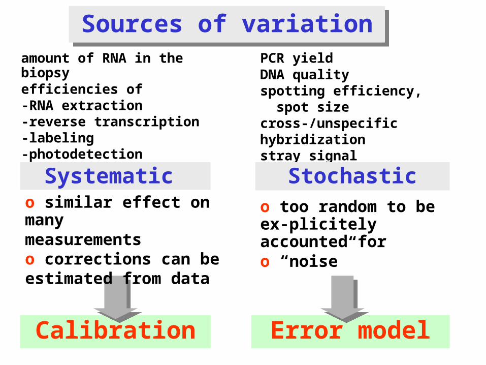
Sources of variationSources of variationamount of RNA in the biopsy efficiencies of-RNA extraction-reverse transcription -labeling-photodetection

PCR yieldDNA qualityspotting efficiency, spot sizecross-/unspecific hybridizationstray signal

Calibration Error model

Systematic o similar effect on many measurementso corrections can be estimated from data

Stochastico too random to be ex-plicitely accounted for o “noise”

iik ika a

ai per-sample offset

ik ~ N(0, bi2s1

2)

“additive noise”

bi per-sample normalization factor

bk sequence-wise probe efficiency

ik ~ N(0,s22)

“multiplicative noise”

exp( )iik k ikb b b

ik ik ik ky a b x

A simple mathematical model

measured intensity = offset + gain true abundance

The two-component model

raw scale log scale

“additive” noise

“multiplicative” noise

B. Durbin, D. Rocke, JCB 2001

variance stabilization

Xu a family of random variables with EXu=u, VarXu=v(u).

Define

var f(Xu ) independent of u

1( )

v( )

x

f x duu

derivation: linear approximation

0 20000 40000 60000

8.0

8.5

9.0

9.5

10

.01

1.0

raw scale

tra

nsf

orm

ed

sca

le

variance stabilization

f(x)

x

variance stabilizing transformations

1( )

v( )

x

f x duu

1.) constant variance

( ) constv u f u

2.) const. coeff. of variation

2( ) logv u u f u

4.) microarray

2 2 00( ) ( ) arsinh

u uv u u u s f

s

3.) offset2

0 0( ) ( ) log( )v u u u f u u

the “glog” transformation

intensity-200 0 200 400 600 800 1000

- - - f(x) = log(x)

——— hs(x) = asinh(x/s)

2arsinh( ) log 1

arsinh log log2 0limx

x x x

x x

P. Munson, 2001

D. Rocke & B. Durbin, ISMB 2002

W. Huber et al., ISMB 2002

evaluation: effects of different data transformationsd

iffere

nce r

ed

-g

reen

rank(average)

What is the bottomline? Detecting differentially transcribed genes

from cDNA array data

o Data: paired tumor/normal tissue from 19 kidney cancers, in color flip duplicates on 38 cDNA slides à 4000 genes.

o 6 different strategies for normalization and quantification of differential abundance

o Calculate for each gene & each method: t-statistics, permutation-p

o For threshold , compare the number of genes the different methods find, #{pi | pi}

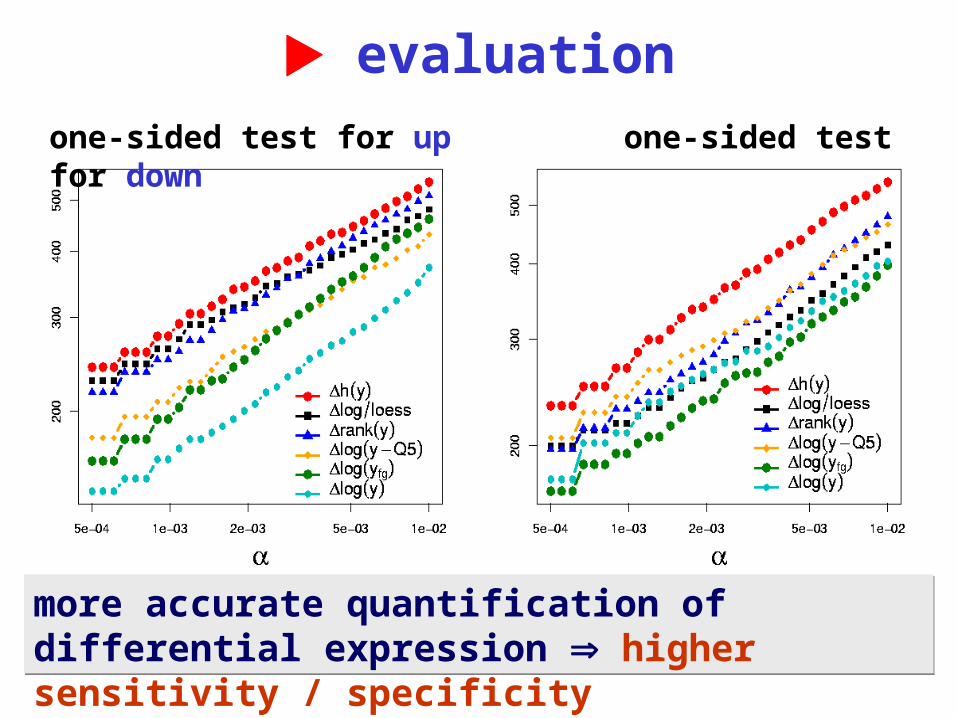
evaluation

more accurate quantification of differential expression higher sensitivity / specificity

one-sided test for up one-sided test for down

Another evaluation: affycomp, a benchmark for Affymetrix genechip expression measures

o Data: Spike-in series: from Affymetrix 59 x HGU95A, 16 genes, 14 concentrations, complex backgroundDilution series: from GeneLogic 60 x HGU95Av2,liver & CNS cRNA in different proportions and amounts

o Benchmark: 15 quality measures regarding-reproducibility-sensitivity -specificity Put together by Rafael Irizarry (Johns Hopkins) http://affycomp.biostat.jhsph.edu

affycomp results (hgu95a chips)good

bad

ROC curves

Availability

Package vsn in Bioconductor:

Preprocessing of two-color, Agilent, and Affymetrix arrays

Candidate gene sets from

microarray studies: dozens…

hundreds

Capacity of detailed in-vivo functional

studies: one…few

How to close the gap?

sample

cro

ss-v

alid

ate

d p

rob

ab

ilitie

s

0 20 40 60

0.0

0.2

0.4

0.6

0.8

1.0

ccRCC chRCC pRCC

Drowning by numbers

How to separate a flood of ‘significant’ secondary effects from causally relevant ones?

VHL: tumor suppressor with “gatekeeper” role in kidney cancers

Boer, Huber, et al. Genome Res. 2001: kidney tumor/normal profiling study

Drowning by numbers

Boer, Huber, et al. Genome Res. 2001

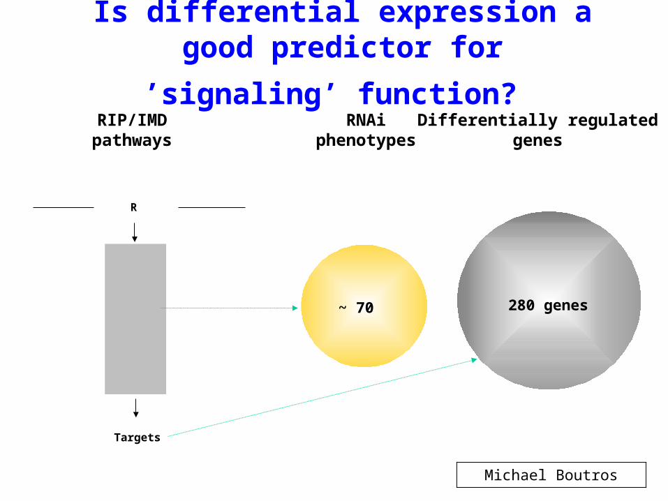
Is differential expression a good

predictor for ’signaling’ function? RNAi

phenotypesDifferentially regulated

genes

~ 70 280 genes

RIP/IMDpathways

RIP

Tak1

IKK

Rel

R

Targets

Michael Boutros

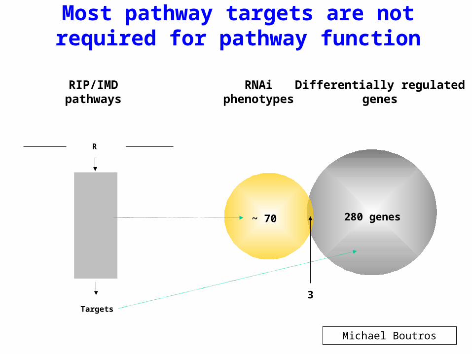
Most pathway targets are not required for pathway function

RNAiphenotypes

Differentially regulatedgenes

~ 70 280 genes

3

RIP/IMDpathways

RIP

Tak1

IKK

Rel

R

Targets

Michael Boutros

Buffering

in yeast, ~73% of gene deletions are "non-essential" (Glaever et al. Nature 418 (2002))

in Drosophila cell lines, only 5% show viability phenotype (Boutros et al. Science 303 (2004))

association studies for most human genetic diseases have failed to produce single loci with high penetrance

evolutionary pressure for robustness

What are the implications for functional studies?

Need to:use combinatorial perturbations

observe multiple phenotypes with high sensitivityunderstand gene-gene and gene-phenotype interactions in

terms of graph-like models ("networks")

From association to intervention

mRNA profiling studies: association of genes with diseases

gene 1disease

gene 2

or or…

the dilemma

oror ?the next step: directed intervention

RNAi+ genome wideo specificity- efficiency / monitoring?

Transfection (expression)+ 100% specific+ monitoring- library size

Small compounds…

Interference/Perturbation tools

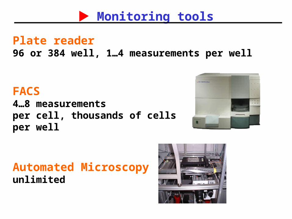
Plate reader96 or 384 well, 1…4 measurements per well

FACS4…8 measurements per cell, thousands of cellsper well

Automated Microscopyunlimited

Monitoring tools

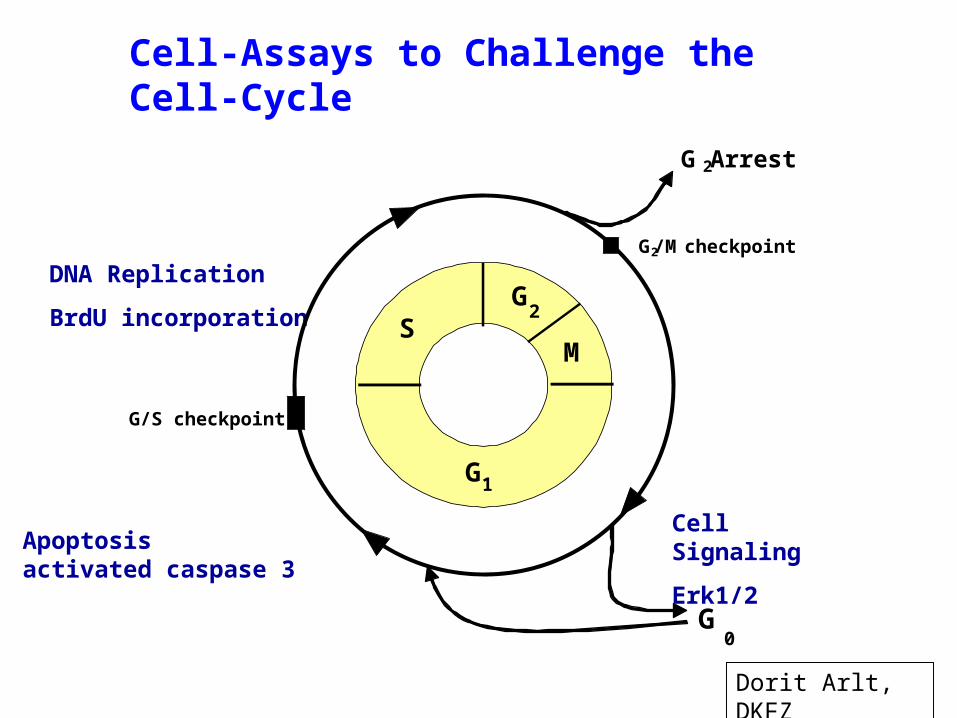
Cell-Assays to Challenge the Cell-Cycle

DNA Replication

BrdU incorporation

G1

G2

M

G/S checkpoint

G2/M checkpoint

G 2 Arrest

G0

S

Apoptosisactivated caspase 3

Cell Signaling

Erk1/2

Dorit Arlt, DKFZ

ORF-YFP Anti-BrdU/Cy5

Proliferation Assay

Measurement of fluorescence intensities

92.6,

2621.8,

1095.4

267.6YFP channel Cy5 channel 72.0 761.0 71.0 684.1 119.7 779.0 87.3 820.2 149.5 645.6 70.2 536.1 84.7 799.5 103.1 912.8 81.0 916.7 2621.8 267.6 74.1 766.2 156.8 866.6 169.0 819.8 105.5 757.7 156.0 367.8 76.5 746.2 135.2 731.2 86.2 567.3 77.7 896.3 92.6 1095.4 104.6 633.3 481.2 567.7 539.0 663.9 95.0 726.2 156.7 842.1

Local Regression analysis

Signal intensity (cyclin A)

… focus on small perturbations and weak phenotypes!

local slope

0

0'

ˆ '( )

ˆ ( )m

m xz

xArlt, Huber, et al. submitted (2005)

Signal intensity (PP2A)

Signal intensity (CFP)

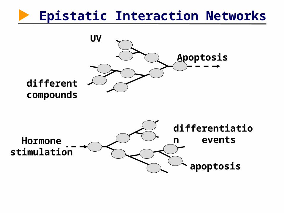
Hormone stimulation

Epistatic Interaction Networks

Apoptosis

differentiation events

apoptosis

UV

different compounds

T1 T2 T3

T3

T2T1

A

B

Gene needed for shape change (Model B)

Gene inhibits cell death or promotes survival (Model B?)

SHAPECHANGE

CYCLEARREST

CELLDEATH

E = Ecdysone stimulus

T = Temporal Response

= Assay for Response

… = assay timepoints

RNAi 2

RNAi 3

Simple

Models

Example

Results?

RNAi 4

RNAi 5

E

E

Gene needed for shape change and cell death (Model A)

Gene needed for cell death (Model A or B)

RNAi +No phenotype

ERNAi1

Epistatic Interaction Networks

A. Kiger UCSD

Basic formal concepts, software, and case studies

Wolfgang Huber, EBI / EMBL

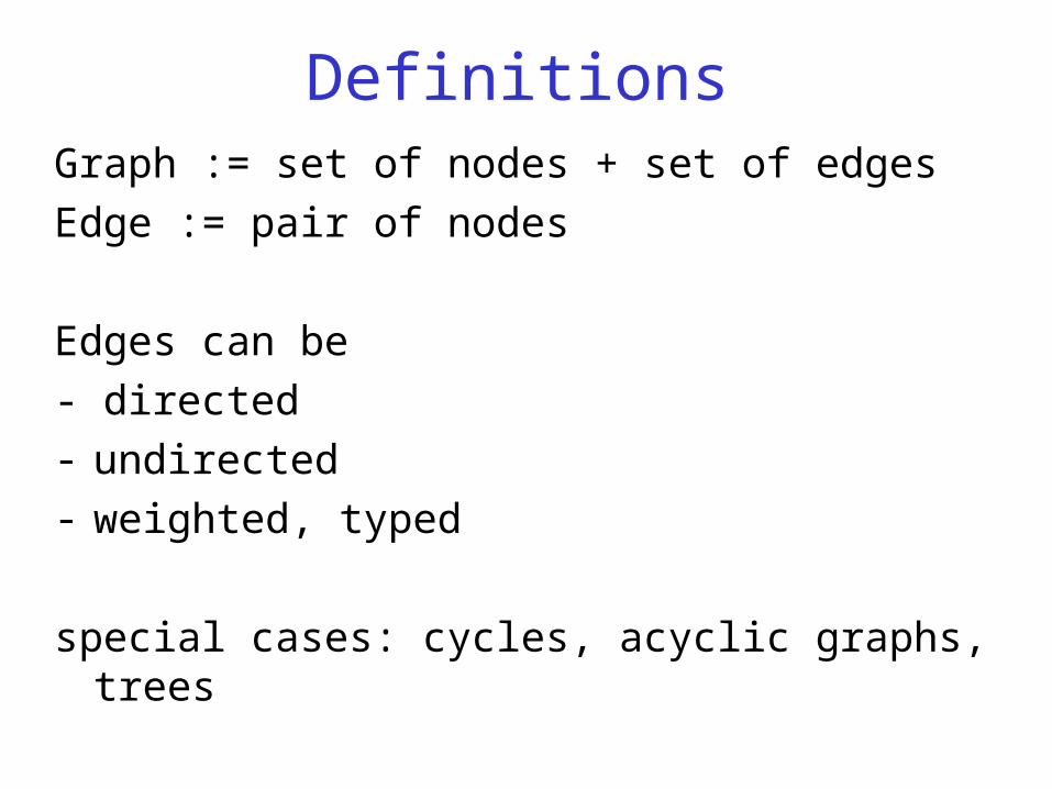
DefinitionsGraph := set of nodes + set of edges

Edge := pair of nodes

Edges can be

- directed- undirected- weighted, typed

special cases: cycles, acyclic graphs, trees

Network topologies

regular all-to-all

Random graph (after "tidy"

rearrangement of nodes)

Network topologies

Scale-free

Random Edge Graphsn nodes, m edges

p(i,j) = 1/m

with high probability:

m < n/2: many disconnected components

m > n/2: one giant connected component: size ~ n.

(next biggest: size ~ log(n)).

degrees of separation: log(n).

Erdös and Rényi 1960

Small worlds

Clustering

Degree distribution

Motifs

Some popular concepts:

Small world networks

Typical path length („degrees of separation“) is short

many examples:

- communications

- epidemiology / infectious diseases

- metabolic networks

- scientific collaboration networks

- WWW

- company ownership in Germany

- „6 degrees of Kevin Bacon“

But not in

- regular networks, random edge graphs

Cliques and clustering coefficient

Clique: every node connected to everyone else

Clustering coefficient:

Random network: E[c]=p

Real networks: c » p

no. edges between first-degree neighbors

maximum possible number of such edgesc

Degree distributions

p(k) = proportion of nodes that have k edges

Random graph: p(k) = Poisson distribution with some parameter („scale“)(„scale“)

Many real networks: p(k) = power law,

p(k) ~ k

„scale-free“

In principle, there could be many other distributions: exponential, normal, …

Growth models for scale free networks

Start out with one node and continously add nodes, with preferential attachment to existing nodes, with probability ~ degree of target node.

p(k)~k-3

(Simon 1955; Barabási, Albert, Jeong 1999)

"The rich get richer"

Modifications to obtain 3:

Through different rules for adding or rewiring of edges, can tune to obtain any kind of degree distribution

Real networks

- tend to have power-law scaling (truncated)

- are ‚small worlds‘ (like random networks)

- have a high clustering coefficient independent of network size (like lattices and unlike random networks)

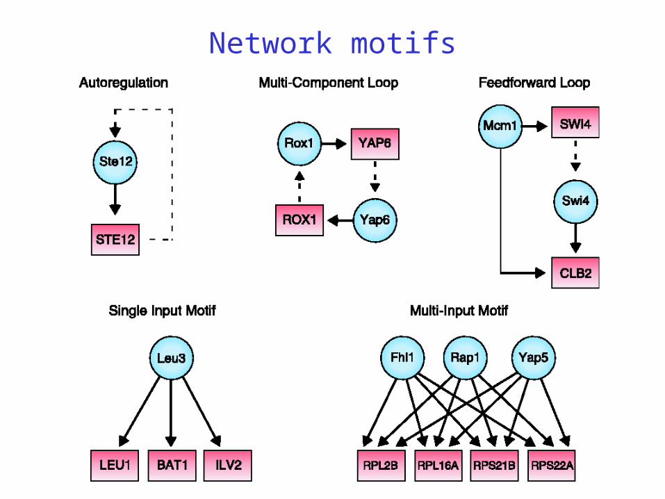
Network motifs

:= pattern that occurs more often than in randomized networks

Intended implications

duplication: useful building blocks are reused by nature

there may be evolutionary pressure for convergence of network architectures

Network motifsStarting point: graph with directed edges

Scan for n-node subgraphs (n=3,4) and count number of occurence

Compare to randomized networks

(randomization preserves in-, out- and in+out- degree of each node, and the frequencies of all (n-1)-subgraphs)

Schematic view of motif detection

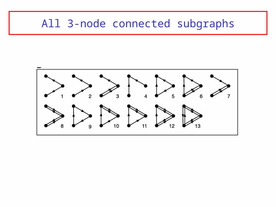
All 3-node connected subgraphs

Transcription networks

Nodes = transcription factors

Directed edge: X regulates transcription of Y

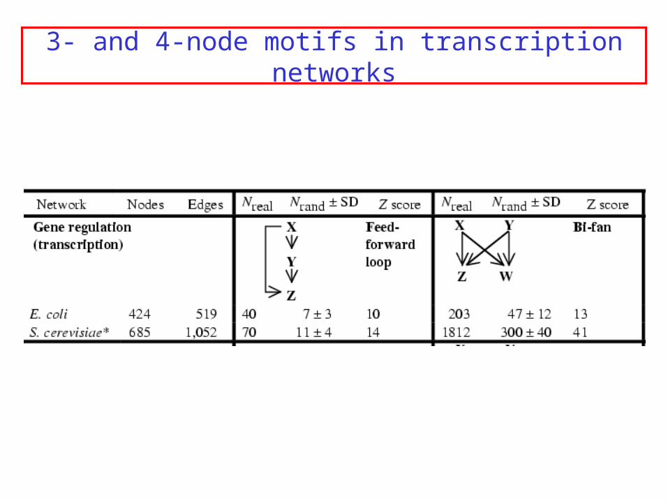
3- and 4-node motifs in transcription networks

Transcriptional regulatory networksfrom "genome-wide location analysis"

regulator := a transcription factor (TF) or a ligand of a TFtag: c-myc epitope

106 microarrayssamples: enriched (tagged-regulator + DNA-promoter)probes: cDNA of all promoter regionsspot intensity ~ affinity of a promotor to a certain regulator

Transcriptional regulatory networksbipartite graph

1

1

1

1

1

1

1

106 regulators (TFs)

6270

pro

mo

ter

reg

ion

s

regulators

promoters

Network motifs

Network motifs

Graphs with R and Bioconductor

graph, RBGL, Rgraphviz

graph basic class definitions and functionality

RBGL interface to graph algorithms (e.g. shortest path, connectivity)

Rgraphviz rendering functionality Different layout algorithms. Node plotting, line type, color etc. can be controlled by the user.

Creating our first graphlibrary(graph); library(Rgraphviz)

edges <- list(a=list(edges=2:3), b=list(edges=2:3), c=list(edges=c(2,4)), d=list(edges=1))

g <- new("graphNEL", nodes=letters[1:4], edgeL=edges, edgemode="directed")

plot(g)

Querying nodes, edges, degree > nodes(g)[1] "a" "b" "c" "d"

> edges(g)$a[1] "b" "c"$b[1] "b" "c"$c[1] "b" "d"$d[1] "a"

> degree(g)$inDegreea b c d1 3 2 1$outDegreea b c d2 2 2 1

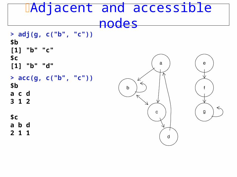
Adjacent and accessible nodes> adj(g, c("b", "c"))$b[1] "b" "c"$c[1] "b" "d"

> acc(g, c("b", "c"))$ba c d3 1 2

$ca b d2 1 1

Undirected graphs, subgraphs, boundary graph

> ug <- ugraph(g)

> plot(ug)

> sg <- subGraph(c("a", "b",

"c", "f"), ug)

> plot(sg)

> boundary(sg, ug)> $a>[1] "d"> $b> character(0)> $c>[1] "d"> $f>[1] "e" "g"

Weighted graphs

> edges <- list(a=list(edges=2:3, weights=1:2),+ b=list(edges=2:3, weights=c(0.5, 1)),+ c=list(edges=c(2,4), weights=c(2:1)),+ d=list(edges=1, weights=3))

> g <- new("graphNEL", nodes=letters[1:4], edgeL=edges, edgemode="directed")

> edgeWeights(g)$a2 31 2$b 2 30.5 1.0$c2 42 1

$d13

Graph manipulation> g1 <- addNode("e", g)

> g2 <- removeNode("d", g)

> ## addEdge(from, to, graph, weights)

> g3 <- addEdge("e", "a", g1, pi/2)

> ## removeEdge(from, to, graph)

> g4 <- removeEdge("e", "a", g3)

> identical(g4, g1)

[1] TRUE

Graph algebra

Random graphs

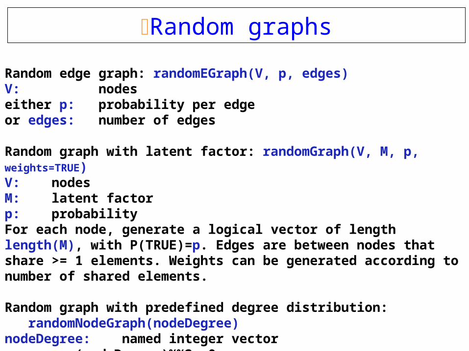
Random edge graph: randomEGraph(V, p, edges)V: nodeseither p: probability per edgeor edges: number of edges

Random graph with latent factor: randomGraph(V, M, p, weights=TRUE)V: nodesM: latent factorp: probabilityFor each node, generate a logical vector of length length(M), with P(TRUE)=p. Edges are between nodes that share >= 1 elements. Weights can be generated according to number of shared elements.

Random graph with predefined degree distribution:randomNodeGraph(nodeDegree)

nodeDegree: named integer vectorsum(nodeDegree)%%2==0

Random edge graph

100 nodes 50 edges

degree distribution

Graph representations

node-edge list: graphNELlist of nodeslist of out-edges for each node

from-to matrix

adjacency matrix

adjacency matrix (sparse) graphAM (to come)

node list + edge list: pNode, pEdge (Rgraphviz)list of nodeslist of edges (node pairs, possibly ordered)

Ragraph: representation of a laid out graph

Graph representations: from-to-matrix

> ft [,1] [,2][1,] 1 2[2,] 2 3[3,] 3 1[4,] 4 4

> ftM2adjM(ft) 1 2 3 41 0 1 0 02 0 0 1 03 1 0 0 04 0 0 0 1

GXL: graph exchange language

<gxl> <graph edgemode="directed" id="G"> <node id="A"/> <node id="B"/> <node id="C"/> … <edge id="e1" from="A" to="C"> <attr name="weights"> <int>1</int> </attr> </edge> <edge id="e2" from="B" to="D"> <attr name="weights"> <int>1</int> </attr> </edge> …</graph></gxl>

from graph/GXL/kmstEx.gxl

GXL (www.gupro.de/GXL)

is "an XML sublanguage

designed to be a standard exchange format for graphs". The graph package

provides tools for im- and exporting

graphs as GXL

RBGL: interface to the Boost Graph Library

Connected componentscc = connComp(rg) table(listLen(cc)) 1 2 3 4 15 18 36 7 3 2 1 1

Choose the largest componentwh = which.max(listLen(cc)) sg = subGraph(cc[[wh]], rg)

Depth first searchdfsres = dfs(sg, node = "N14")nodes(sg)[dfsres$discovered] [1] "N14" "N94" "N40" "N69" "N02" "N67" "N45" "N53" [9] "N28" "N46" "N51" "N64" "N07" "N19" "N37" "N35" [17] "N48" "N09"

rg

depth / breadth first search

dfs(sg, "N14")bfs(sg, "N14")

connected components

sc = strongComp(g2)

nattrs = makeNodeAttrs(g2, fillcolor="")

for(i in 1:length(sc)) nattrs$fillcolor[sc[[i]]] =

myColors[i]

plot(g2, "dot", nodeAttrs=nattrs)

wc = connComp(g2)

minimal spanning tree

km <- fromGXL(file(system.file("GXL/kmstEx.gxl", package = "graph")))

ms <- mstree.kruskal(km)

e <- buildEdgeList(km)n <- buildNodeList(km)

for(i in 1:ncol(ms$edgeList))

e[[paste(ms$nodes[ms$edgeList[,i]], collapse="~")]]@attrs$color

<- "red"

z <- agopen(nodes=n, edges=e, edgeMode="directed", name="")

plot(z)

shortest path algorithms

Different algorithms for different types of graphs o all edge weights the sameo positive edge weightso real numbers

…and different settings of the problemo single pairo single sourceo single destinationo all pairs

Functionsbfsdijkstra.spsp.betweenjohnson.all.pairs.sp

shortest path

1

set.seed(123)rg2 = randomEGraph(nodeNames, edges = 100)fromNode = "N43"toNode = "N81"sp = sp.between(rg2,

fromNode, toNode)

sp[[1]]$path [1] "N43" "N08" "N88" [4] "N73" "N50" "N89" [7] "N64" "N93" "N32" [10] "N12" "N81"

sp[[1]]$length [1] 10

shortest path

ap = johnson.all.pairs.sp(rg2)hist(ap)

minimal spanning tree

mst = mstree.kruskal(gr)gr

connectivity

Consider graph g with single connected component.Edge connectivity of g: minimum number of edges in g that can be cut to produce a graph with two components. Minimum disconnecting set: the set of edges in this cut.

> edgeConnectivity(g)$connectivity[1] 2

$minDisconSet$minDisconSet[[1]][1] "D" "E"

$minDisconSet[[2]][1] "D" "H"

Rgraphviz: the different layout engines

dot: directed graphs. Works best on DAGs and other graphs that can be drawn as hierarchies.

neato: undirected graphs using ’spring’ models

twopi: radial layout. One node (‘root’) chosen as the center. Remaining nodes on a sequence of concentric circles about the origin, with radial distance proportional to graph distance. Root can be specified or chosen heuristically.

Rgraphviz: the different layout engines

Rgraphviz: the different layout engines

domain combination graph

ImageMap

lg = agopen(g, …)

imageMap(lg, con=file("imca-frame1.html", open="w") tags= list(HREF = href, TITLE = title, TARGET = rep("frame2", length(AgNode(nag)))), imgname=fpng, width=imw, height=imh)

Show drosophila interaction network example

Using GO to interprete gene lists

Using GO to interprete gene lists

Packages: Gostats, Rgraphviz

A pathway graph

A pathway graph

Probabilistic tree model for DNA copy number data (matrix CGH).

oncotree package by Anja von Heydebreck

Acknowledgements

R project: R-core teamwww.r-project.org

Bioconductor project: Robert Gentleman, Vince Carey, Jeff Gentry, and many otherswww.bioconductor.org

graphviz project: Emden Gansner, Stephen North, Yehuda Koren (AT&T Research)www.graphviz.org

Boost graph library: Jeremy Siek, Lie-Quan Lee, Andrew Lumsdaine, Indiana Universitywww.boost.org/libs/graph/doc

References

Can a biologist fix a radio? Y. Lazebnik, Cancer Cell 2:179 (2002)

Social Network Analysis, Methods and Applications. S. Wasserman and K. Faust, Cambridge University Press (1994)

Bioinformatics and Computational Biology Solutions using R and Bioconductor. R. Gentleman, V. Carey, W. Huber, R. Irizarry, S. Dudoit. Springer, available in summer 2005.