Embed Size (px)
Citation preview
Boris AltshulerColumbia University
NEC Laboratories America
From Quantum ChaosFrom Quantum ChaosTo To
Anderson Localization Anderson Localization

RANDOM MATRICES
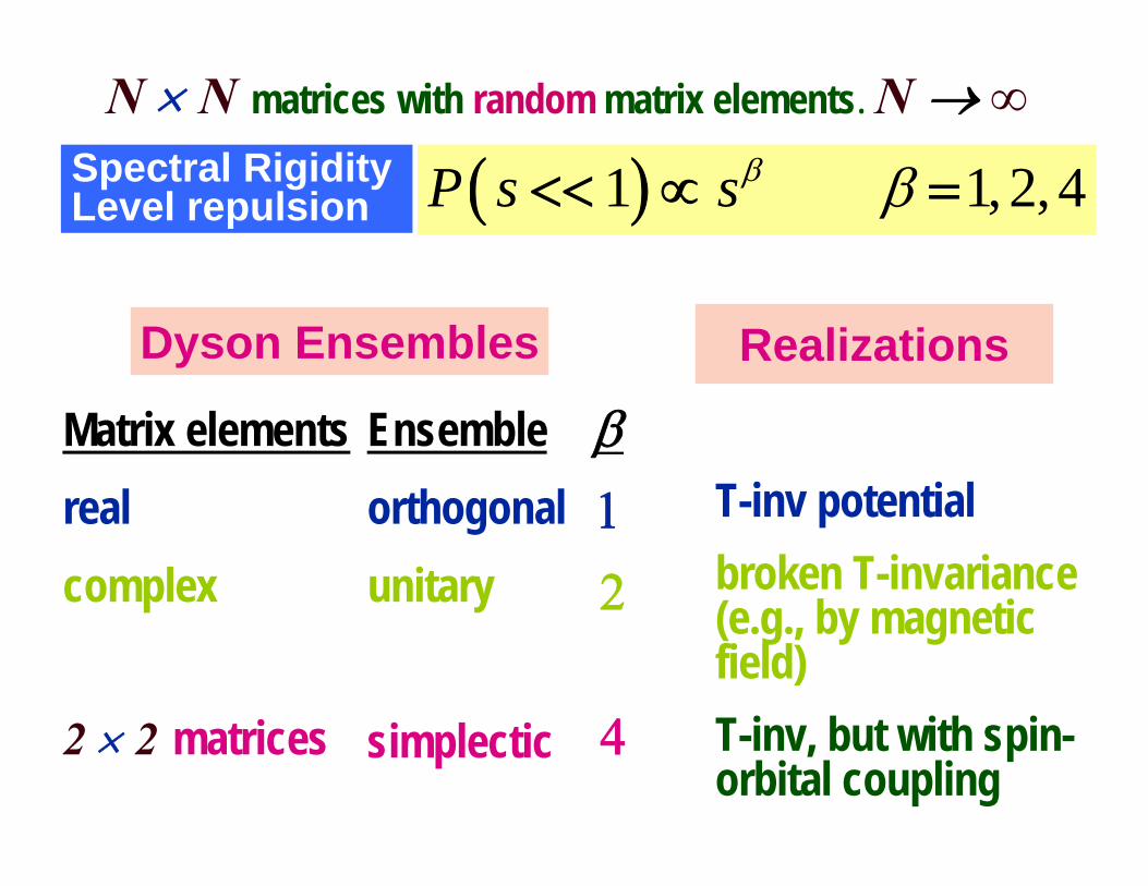
N × N matrices with random matrix elements. N → ∞
Ensembleorthogonalunitarysimplectic
Dyson Ensembles
Matrix elementsrealcomplex
2 × 2 matrices
RANDOM MATRIX THEORY
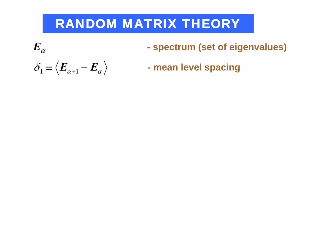
Eα - spectrum (set of eigenvalues)
- mean level spacingααδ EE −≡ +11

RANDOM MATRIX THEORY
Eα - spectrum (set of eigenvalues)
- mean level spacing
- ensemble averaging
ααδ EE −≡ +11
......

RANDOM MATRIX THEORY
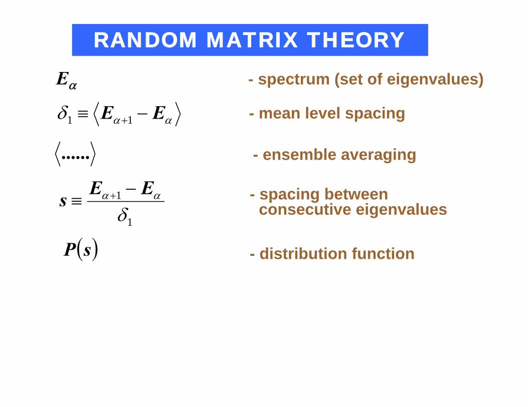
Eα - spectrum (set of eigenvalues)
- mean level spacing
- ensemble averaging
1
1
δαα EEs −
≡ +
ααδ EE −≡ +11
......
- spacing between consecutive eigenvalues
RANDOM MATRIX THEORY
Eα - spectrum (set of eigenvalues)
- mean level spacing
- ensemble averaging
( )sP1
1
δαα EEs −
≡ +
ααδ EE −≡ +11
......
- spacing between consecutive eigenvalues
- distribution function
RANDOM MATRIX THEORY
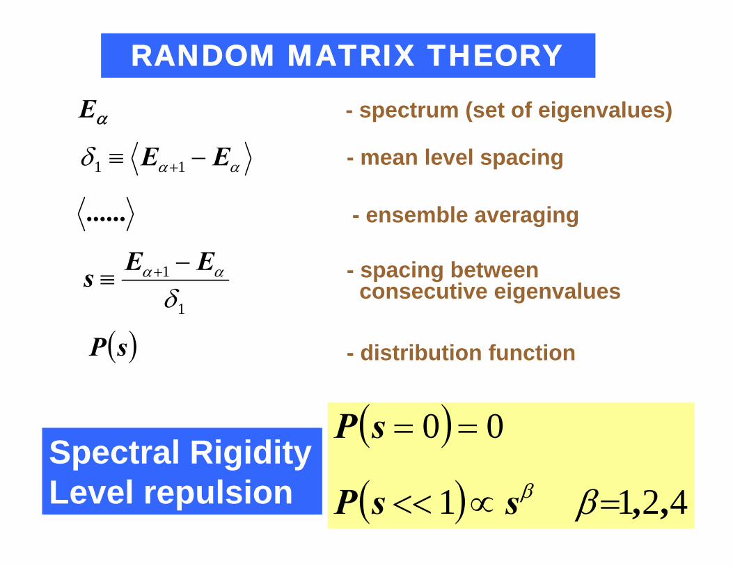
Eα - spectrum (set of eigenvalues)
- mean level spacing
- ensemble averaging
- spacing between consecutive eigenvalues
- distribution function
Spectral RigidityLevel repulsion
( )
( ) 4211
00
,,=∝<<
==
ββssP
sP
( )sP1
1
δαα EEs −
≡ +
ααδ EE −≡ +11
......

Noncrossing rule (theorem)Suggested by Hund (Hund F. 1927 Phys. v.40, p.742)
Justified by von Neumann & Wigner (v. Neumann J. & Wigner E.1929 Phys. Zeit. v.30, p.467) . . . .
Usually textbooks present a simplified version of the justification due to Teller (Teller E., 1937 J. Phys. Chem 41 109).
Arnold V. I., 1972 Funct. Anal. Appl.v. 6, p.94
Mathematical Methods of Classical Mechanics (Springer-Verlag: New York), Appendix 10, 1989
( )0 0P s = =

In general, a multiple spectrum in typical families of quadratic forms is observed only for two or more parameters, while in one-parameter families of general form the spectrum is simple for all values of the parameter. Under a change of parameter in the typical one-parameter family the eigenvalues can approach closely, but when they are sufficiently close, it is as if they begin to repel one another. The eigenvalues again diverge, disappointing the person who hoped, by changing the parameter to achieve a multiple spectrum.
Arnold V.IArnold V.I., Mathematical Methods of Classical Mechanics (Springer-Verlag: New York), Appendix 10, 1989
( ) ( )H x E xα⇒

In general, a multiple spectrum in typical families of quadratic forms is observed only for two or more parameters, while in one-parameter families of general form the spectrum is simple for all values of the parameter. Under a change of parameter in the typical one-parameter family the eigenvalues can approach closely, but when they are sufficiently close, it is as if they begin to repel one another. The eigenvalues again diverge, disappointing the person who hoped, by changing the parameter to achieve a multiple spectrum.
Arnold V.I., Mathematical Methods of Classical Mechanics (Springer-Verlag: New York), Appendix 10, 1989
E
x
( ) ( )H x E xα⇒

1. The assumption is that the matrix elements are statistically independent. Therefore probability of two levels to be degenerate vanishes.
2. If H12 is real (orthogonal ensemble), then for s to be small two statistically independent variables ((H22- H11) and H12) should be small and thus
( ) 0P s → 0 :s →Reason for when
11 12
12 22
ˆH H
HH H∗
⎛ ⎞⎜ ⎟=⎜ ⎟⎝ ⎠
( )2 22 1 22 11 12E E H H H− = − +
small small small
( ) 1P s s β∝ =
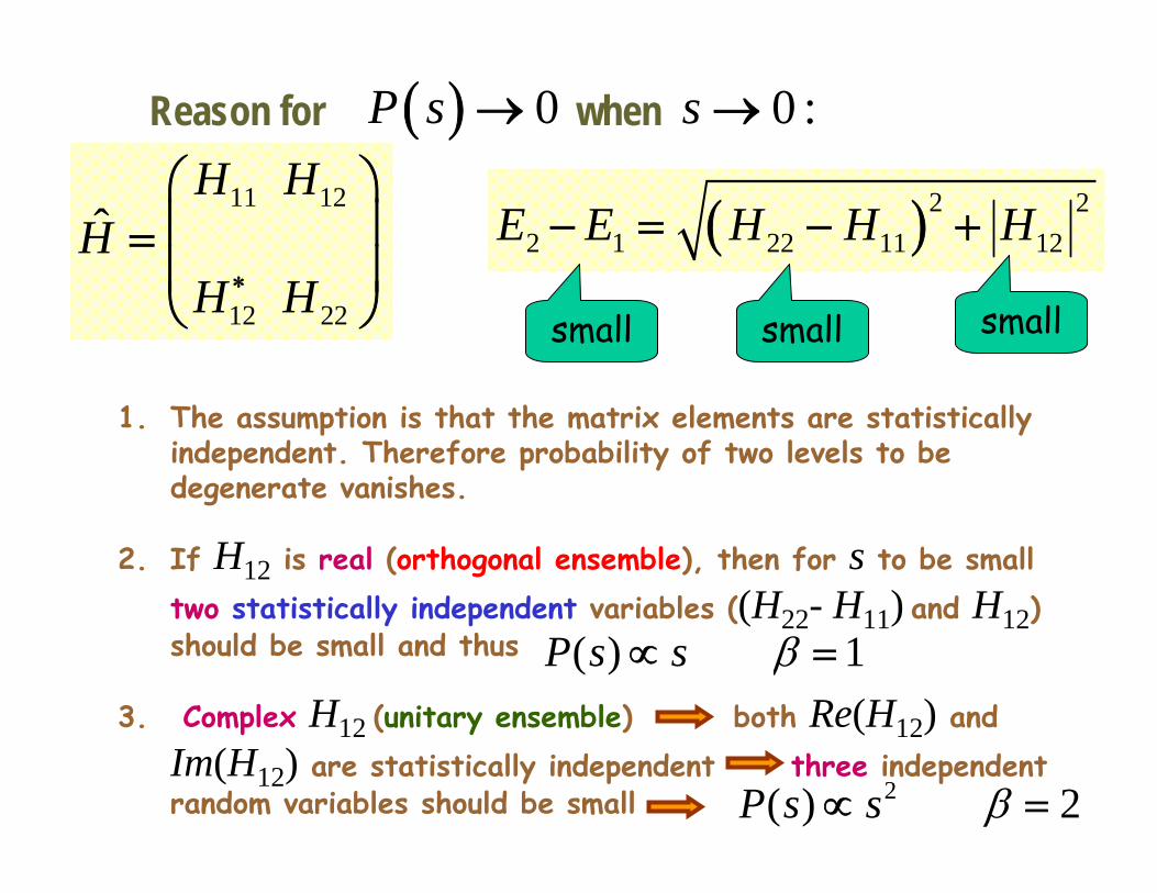
1. The assumption is that the matrix elements are statistically independent. Therefore probability of two levels to be degenerate vanishes.
2. If H12 is real (orthogonal ensemble), then for s to be small two statistically independent variables ((H22- H11) and H12) should be small and thus
3. Complex H12 (unitary ensemble) both Re(H12) and Im(H12) are statistically independent three independent random variables should be small
( ) 0P s → 0 :s →Reason for when
11 12
12 22
ˆH H
HH H∗
⎛ ⎞⎜ ⎟=⎜ ⎟⎝ ⎠
( )2 22 1 22 11 12E E H H H− = − +
small small small
( ) 1P s s β∝ =
2( ) 2P s s β∝ =

Poisson – completely uncorrelated levels
Wigner-Dyson; GOEPoisson
GaussianOrthogonalEnsemble
Orthogonal β=1
Unitaryβ=2
Simplecticβ=4
N × N matrices with random matrix elements. N → ∞
Ensembleorthogonalunitary
simplectic
Dyson Ensembles
β 1
2
4
T-inv potentialbroken T-invariance (e.g., by magnetic field)T-inv, but with spin-orbital coupling
Matrix elementsrealcomplex
2 × 2 matrices
Spectral Rigidity Level repulsion ( )1 1,2, 4P s sβ β<< ∝ =
Realizations

Finite size quantum physical systems
AtomsNucleiMolecules...
Quantum Dots

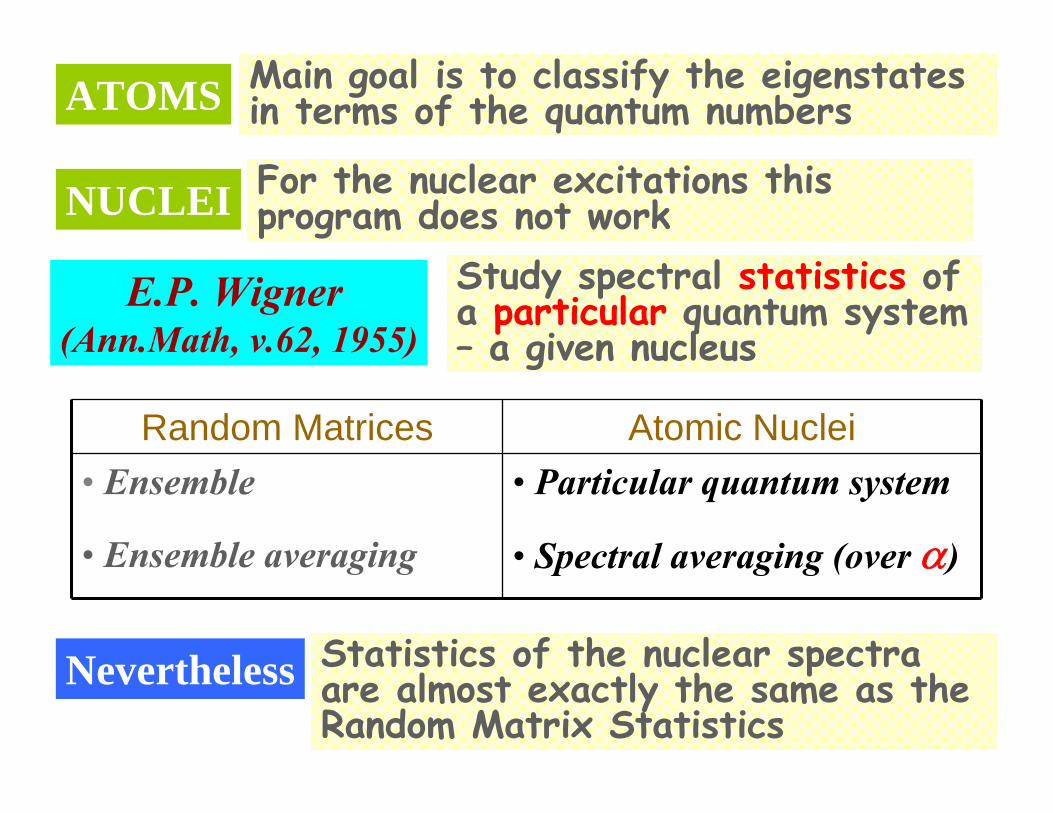
ATOMS
NUCLEI
Main goal is to classify the eigenstates in terms of the quantum numbers
For the nuclear excitations this program does not work
N. Bohr, Nature 137 (1936) 344.

ATOMS
NUCLEI
Main goal is to classify the eigenstates in terms of the quantum numbers
For the nuclear excitations this program does not work
E.P. Wigner(Ann.Math, v.62, 1955)
Study spectral statistics of a particular quantum system – a given nucleus
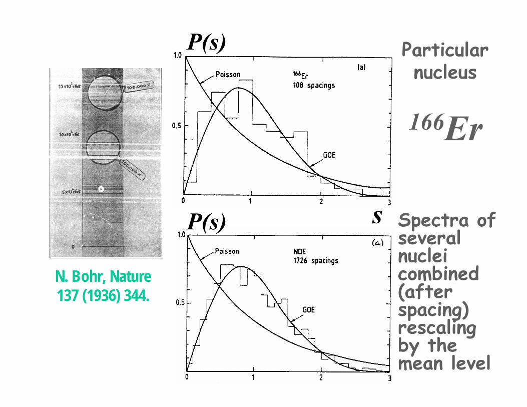
sP(s)
Particular nucleus
166Er
Spectra of several nuclei combined (after spacing)rescaling by the mean level
P(s)
N. Bohr, Nature 137 (1936) 344.
ATOMS
NUCLEI
Main goal is to classify the eigenstates in terms of the quantum numbers
For the nuclear excitations this program does not work
E.P. Wigner(Ann.Math, v.62, 1955)
Study spectral statistics of a particular quantum system – a given nucleus
• Particular quantum system
• Spectral averaging (over α)
• Ensemble
• Ensemble averaging
Atomic NucleiRandom Matrices
Nevertheless Statistics of the nuclear spectra are almost exactly the same as the Random Matrix Statistics

T-invariance (CP) violation – crossover between Orthogonal and Unitary ensembles

Q: Why the random matrix theory (RMT) works so well for nuclear spectra
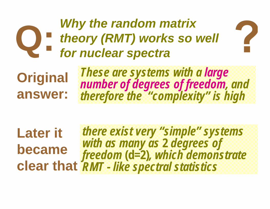
Q: Why the random matrix theory (RMT) works so well for nuclear spectra
Original answer:
These are systems with a large number of degrees of freedom, and therefore the “complexity” is high
Later itbecameclear that
there exist very “simple” systems with as many as 2 degrees of freedom (d=2), which demonstrate RMT - like spectral statistics

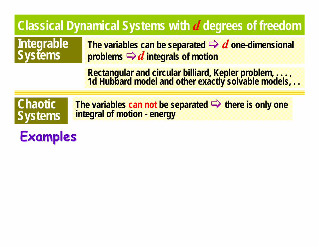
Integrable Systems
Classical Dynamical Systems with d degrees of freedomThe variables can be separated and the problem reduces to d one-dimensional problems
d integrals of motion

Integrable Systems
Classical (h =0) Dynamical Systems with d degrees of freedomThe variables can be separated and the problem reduces to d one-dimensional problems
d integrals of motion
ExamplesExamples1. A ball inside rectangular billiard; d=2• Vertical motion can be
separated from the horizontal one
• Vertical and horizontalcomponents of the
momentum, are both integrals of motion
2. Circular billiard; d=2• Radial motion can be
separated from the angular one
• Angular momentum and energy are the integrals of motion

Integrable Systems
Classical Dynamical Systems with d degrees of freedom
Rectangular and circular billiard, Kepler problem, . . . , 1d Hubbard model and other exactly solvable models, . .
The variables can be separated d one-dimensional problems d integrals of motion
Integrable Systems
Classical Dynamical Systems with d degrees of freedom
Rectangular and circular billiard, Kepler problem, . . . , 1d Hubbard model and other exactly solvable models, . .
The variables can be separated d one-dimensional problems d integrals of motion
Chaotic Systems
The variables can not be separated there is only one integral of motion - energy
ExamplesExamples

Integrable Systems
Classical Dynamical Systems with d degrees of freedom
Rectangular and circular billiard, Kepler problem, . . . , 1d Hubbard model and other exactly solvable models, . .
The variables can be separated d one-dimensional problems d integrals of motion
Chaotic Systems
The variables can not be separated there is only one integral of motion - energy
Stadium
ExamplesExamples

Integrable Systems
Classical Dynamical Systems with d degrees of freedom
Rectangular and circular billiard, Kepler problem, . . . , 1d Hubbard model and other exactly solvable models, . .
The variables can be separated d one-dimensional problems d integrals of motion
Chaotic Systems
The variables can not be separated there is only one integral of motion - energy
ExamplesExamples
Stadium

Stadium
Integrable Systems
Classical Dynamical Systems with d degrees of freedom
Rectangular and circular billiard, Kepler problem, . . . , 1d Hubbard model and other exactly solvable models, . .
The variables can be separated d one-dimensional problems d integrals of motion
Chaotic Systems
The variables can not be separated there is only one integral of motion - energy
ExamplesExamples
Sinai billiard
Kepler problem in magnetic field
B

Stadium
Chaotic Systems
The variables can not be separated there is only one integral of motion - energy
ExamplesExamples
Sinai billiard
Kepler problem in magnetic field
B
Yakov Sinai Johnnes KeplerLeonid Bunimovich

Classical Chaos h =0
•Nonlinearities•Lyapunov exponents•Exponential dependence on the original conditions
•Ergodicity
Q: What does it mean Quantum Chaos ?
Quantum description of any System Quantum description of any System with a finite number of the degrees with a finite number of the degrees of freedom is a linear problem of freedom is a linear problem ––Shrodinger equation Shrodinger equation
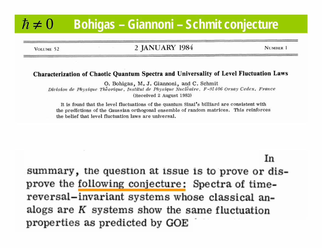
Bohigas – Giannoni – Schmit conjecture0≠h
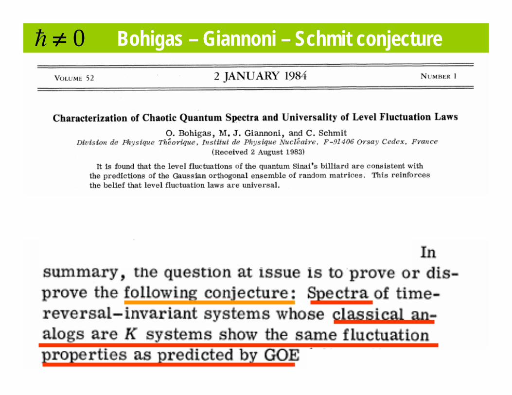
Bohigas – Giannoni – Schmit conjecture0≠h

Bohigas – Giannoni – Schmit conjecture
Chaotic classical analog
Wigner- Dyson spectral statistics
0≠h
No quantum numbers except
energy

Chaoticclassical analog
Two possible definitions
Wigner -Dyson-like spectrum
Q: What does it mean Quantum Chaos ?

Wigner-Dyson
?Classical
Poisson
Quantum
?Chaotic
Integrable
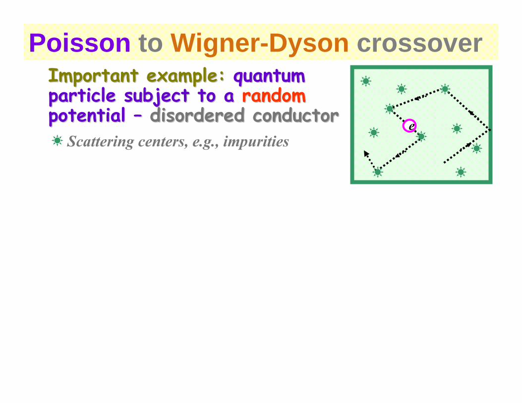
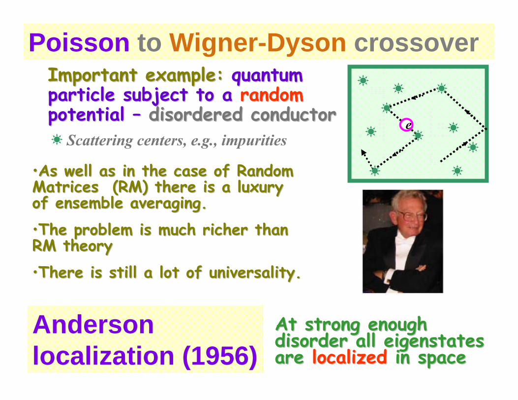
Poisson to Wigner-Dyson crossoverImportant example:Important example: quantum quantum particle subject to a particle subject to a randomrandompotential potential –– disordered conductordisordered conductor e
Scattering centers, e.g., impurities
Poisson to Wigner-Dyson crossoverImportant example:Important example: quantum quantum particle subject to a particle subject to a randomrandompotential potential –– disordered conductordisordered conductor e
Scattering centers, e.g., impurities
••As well as in the case of Random As well as in the case of Random Matrices Matrices (RM) there is a luxury (RM) there is a luxury of ensemble averaging.of ensemble averaging.
••The problem is much richer than The problem is much richer than RM theoryRM theory
••There is still a lot of universality.There is still a lot of universality.
Anderson localization (1956)
At strong enough At strong enough disorder all eigenstates disorder all eigenstates are are localizedlocalized in spacein space

Anderson Insulator Anderson Metal
f = 3.04 GHz f = 7.33 GHz

Poisson to Wigner-Dyson crossoverImportant example:Important example: quantum quantum particle subject to a particle subject to a randomrandompotential potential –– disordered conductordisordered conductor e
Scattering centers, e.g., impurities
Models of disorder:Models of disorder:Randomly located impuritiesRandomly located impurities ( )( ) i
i
U r u r r= −∑r r r
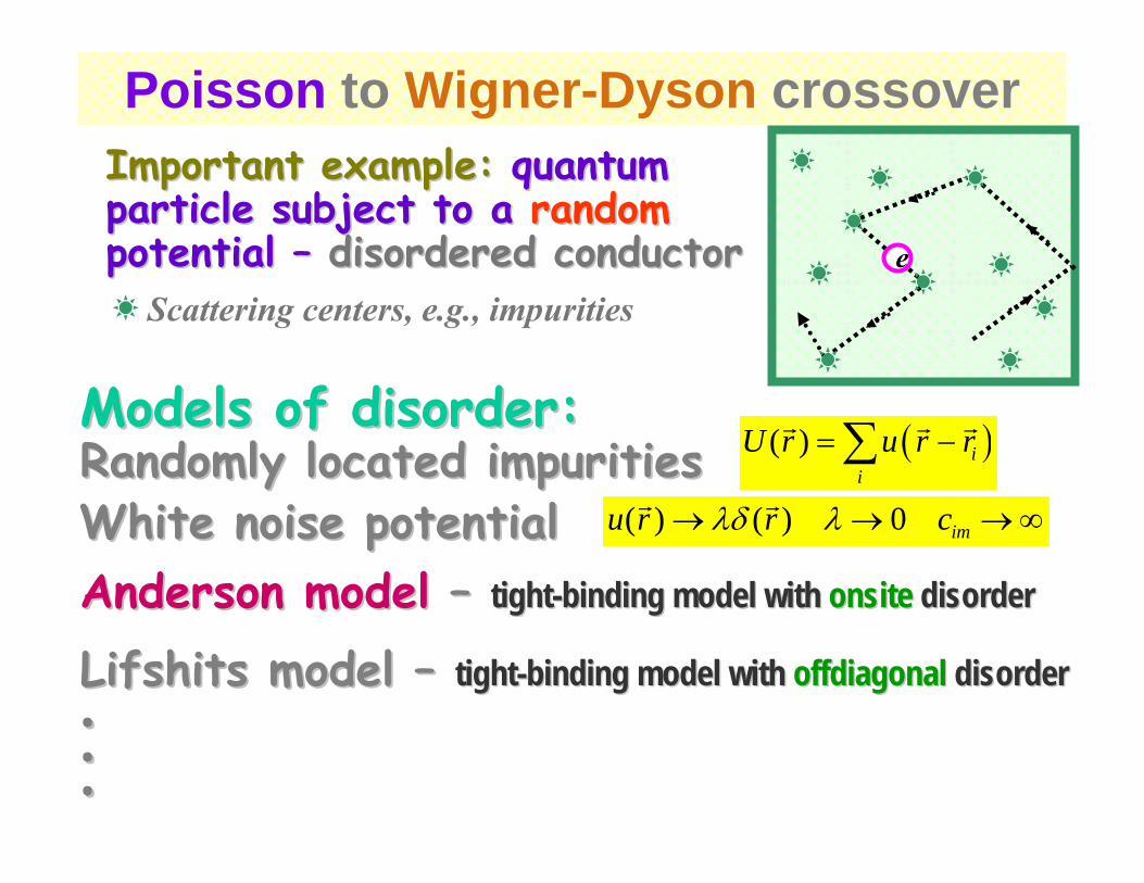
White noise potentialWhite noise potential ( ) ( ) 0 imu r r cλδ λ→ → → ∞r r
Anderson modelAnderson model –– tighttight--binding model with binding model with onsiteonsite disorderdisorder
Lifshits model Lifshits model –– tighttight--binding model with binding model with offdiagonaloffdiagonal disorderdisorder......
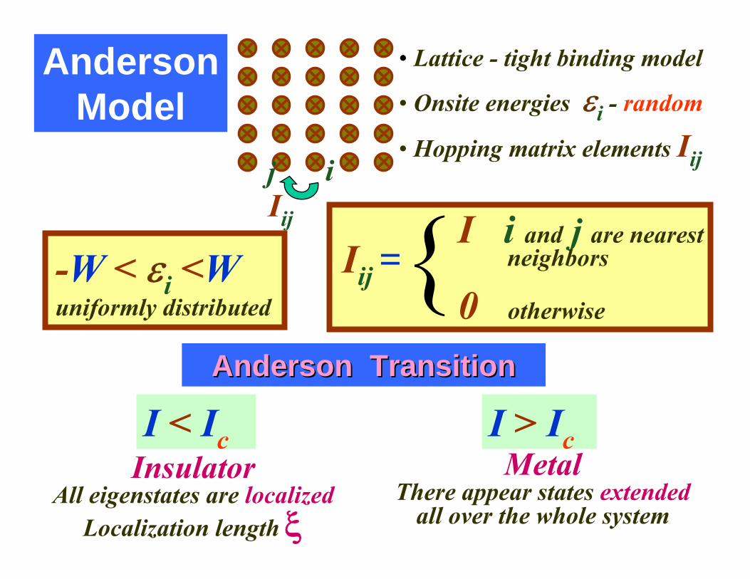
Anderson Model
• Lattice - tight binding model
• Onsite energies εi - random
• Hopping matrix elements Iijj iIij
Iij =I i and j are nearest
neighbors
0 otherwise-W < εi <Wuniformly distributed
I < Ic I > IcInsulator
All eigenstates are localizedLocalization length ξ
MetalThere appear states extended
all over the whole system
Anderson TransitionAnderson Transition
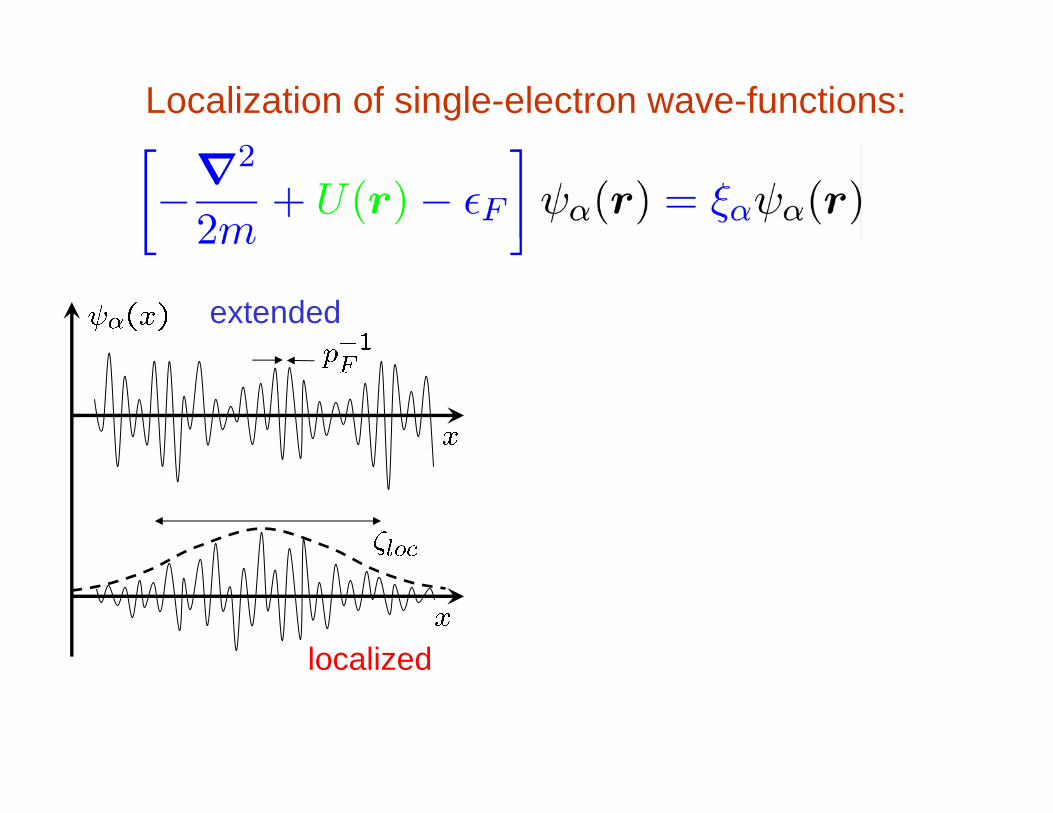
Localization of single-electron wave-functions:
extended
localized
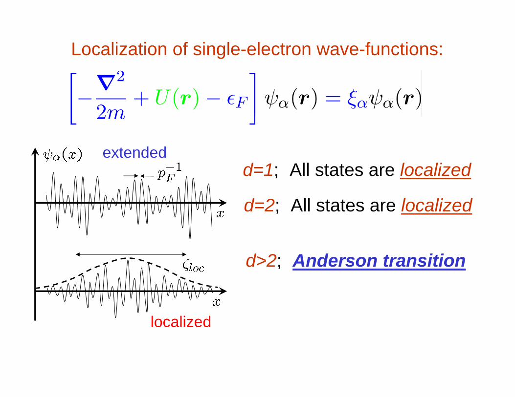
Localization of single-electron wave-functions:
extended
localized
d=1; All states are localized
d=2; All states are localized
d>2; Anderson transition

I < Ic I > IcInsulator
All eigenstates are localizedLocalization length ξ
MetalThere appear states extended
all over the whole system
Anderson TransitionAnderson Transition
The eigenstates, which are localized at different places
will not repel each other
Any two extended eigenstates repel each other
Poisson spectral statistics Wigner – Dyson spectral statistics

Disorder W
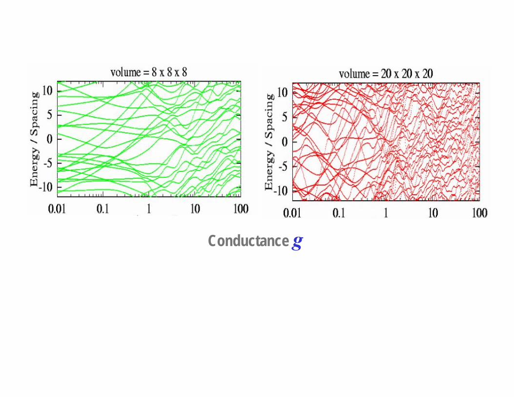
Zharekeschev & Kramer.Exact diagonalization of the Anderson model
( ) ( ) 02
2
=⎥⎦
⎤⎢⎣
⎡−+
∇− rrWU
mrr
αα ψε

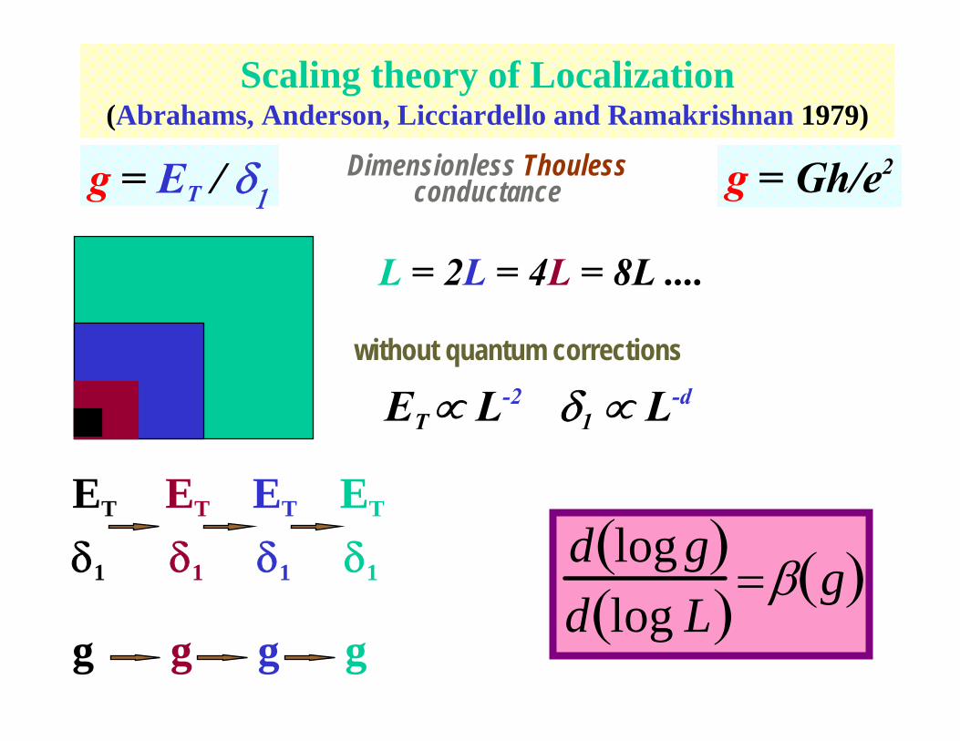
1.1. Mean level spacingMean level spacing δ1 = 1/ν× Ld
2.2. Thouless energyThouless energy ET = hD/L2 D is the diffusion const
. ET has a meaning of the inverse diffusion time of the traveling through the system or the escape rate (for open systems)
dimensionlessThouless
conductanceg = Gh/e2
δ1
ene r
gy
L is the system size;
d is the number ofdimensions
L
g = ET / δ1
Quantum particle in a random potentialQuantum particle in a random potential ((Thouless, 1972))Energy scales

The same statistics of the random spectra and one-particle wave functions
(eigenvectors)
g10
Localized states Insulator
Extended states Metal
Poisson spectralstatistics
Wigner-Dysonspectral statistics
Ν × ΝRandom Matrices
Quantum Dots with Thouless
conductance g
Ν→ ∞ g→ ∞
Thouless Conductance andOne-particle Spectral Statistics

Scaling theory of Localization(Abrahams, Anderson, Licciardello and Ramakrishnan 1979)
L = 2L = 4L = 8L ....
ET ∝ L-2 δ1 ∝ L-d
without quantum corrections
g = Gh/e2g = ET / δ1Dimensionless Thouless
conductance
Scaling theory of Localization(Abrahams, Anderson, Licciardello and Ramakrishnan 1979)
L = 2L = 4L = 8L ....
ET ∝ L-2 δ1 ∝ L-d
without quantum corrections
ET ET ET ET
δ1 δ1 δ1 δ1
g g g g
d log g( )d log L( )=β g( )
g = Gh/e2g = ET / δ1Dimensionless Thouless
conductance

β - function ( )gLdgd β=
loglog
β(g)
g
3D
2D
1D-1
11≈cg
unstablefixed point
Metal – insulator transition in 3DAll states are localized for d=1,2
Conductance g

Anderson transition in terms of pure level statistics
P(s)

Squarebilliard
Sinaibilliard
Disordered localized
Disordered extended
Integrable ChaoticAll chaotic systems resemble each other.
All integrable systems are integrable in their own way

Disordered Systems:
11 >> gET ;δ
11 << gET ;δ
Is it a generic scenario for the Wigner-Dyson to Poisson crossoverQ: ?
Speculations
Anderson metal; Wigner-Dyson spectral statistics
Anderson insulator; Poisson spectral statistics
Consider an integrable system. Each state is characterized by a set of quantum numbers.
It can be viewed as a point in the space of quantum numbers. The whole set of the states forms a lattice in this space.
A perturbation that violates the integrability provides matrix elements of the hopping between different sites (Anderson model !?)
Weak enough hopping - Localization - PoissonStrong hopping - transition to Wigner-Dyson
Does Anderson localization provide a generic scenario for the Wigner-Dyson to Poisson crossover
Q: ?

The very definition of the localization is not invariant – one should specify in which space the eigenstates are localized.
Level statistics is invariant:
Poissonian statistics
basis where the eigenfunctions are localized∃
Wigner -Dyson statistics ∀basis the eigenfunctions
are extended

e
Example 1 Doped semiconductorLow concentration of donors
Electrons are localized on donors Poisson
Higher donorconcentration
Electronic states are extended Wigner-Dyson
Ly
e
Example 1 Doped semiconductorLow concentration of donors
Electrons are localized on donors Poisson
Higher donorconcentration
Electronic states are extended Wigner-Dyson
Example 2Rectangular billiard
Lx
Two integrals of motion x
yx
x Lmp
Lnp ππ
== ;
Lattice in the momentum spacepy
px
Line (surface) of constant energy Ideal billiard – localization in the
momentum spacePoisson
Deformation or smooth random potential
– delocalization in the momentum space
Wigner-Dyson

Localization and diffusion in the angular momentum space
Ra
≡ε 0>ε
0→ε
Chaoticstadium
Integrable circular billiard
1;0 <<= εh
Diffusion in the angular momentum space 25ε∝D
Angular momentum is the integral of motion
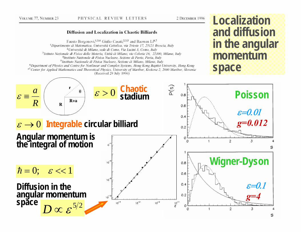
Localization and diffusion in the angular momentum space
Ra
≡ε 0>ε
0→ε
Chaoticstadium
Integrable circular billiard
1;0 <<= εh
Diffusion in the angular momentum space 25ε∝D
Angular momentum is the integral of motion
ε=0.01g=0.012
ε=0.1g=4
Poisson
Wigner-Dyson
D.Poilblanc, T.Ziman, J.Bellisard, F.Mila & G.MontambauxEurophysics Letters, v.22, p.537, 1993
1D Hubbard Model on a periodic chain( ) ∑∑∑
′′+−
+++
+ +++=σσ
σσσ
σσσ
σσσσ,,
,1,,
,,,
,,1,1,i
iii
iii
iiii nnVnnUcccctH
Onsite interaction
n. neighboursinteraction
Hubbard model integrable0=V
extended Hubbard
modelnonintegrable0≠V

1D Hubbard Model on a periodic chain( ) ∑∑∑
′′+−
+++
+ +++=σσ
σσσ
σσσ
σσσσ,,
,1,,
,,,
,,1,1,i
iii
iii
iiii nnVnnUcccctH
Onsite interaction
n. neighbors interaction
Hubbard model integrable0=V
extended Hubbard
modelnonintegrable0≠V
12 sites3 particlesZero total spinTotal momentum π/6
U=4 V=0 U=4 V=4
D.Poilblanc, T.Ziman, J.Bellisard, F.Mila & G.MontambauxEurophysics Letters, v.22, p.537, 1993

D.Poilblanc, T.Ziman, J.Bellisard, F.Mila & G.MontambauxEurophysics Letters, v.22, p.537, 1993
1D t-J model on a periodic chain
t
J exchange
hopping

D.Poilblanc, T.Ziman, J.Bellisard, F.Mila & G.MontambauxEurophysics Letters, v.22, p.537, 1993
1D t-J model on a periodic chain
t
J
forbidden
exchange
hopping
1d t-Jmodel

J=t J=2t J=5t
N=16; one hole
D.Poilblanc, T.Ziman, J.Bellisard, F.Mila & G.MontambauxEurophysics Letters, v.22, p.537, 1993
1D t-J model on a periodic chain
t
J
forbidden
exchange
hopping
1d t-Jmodel

Chaos in Nuclei – Delocalization?
Fermi Sea
generations1 2 3 4 5 6
. . . .Delocalization in Fock space