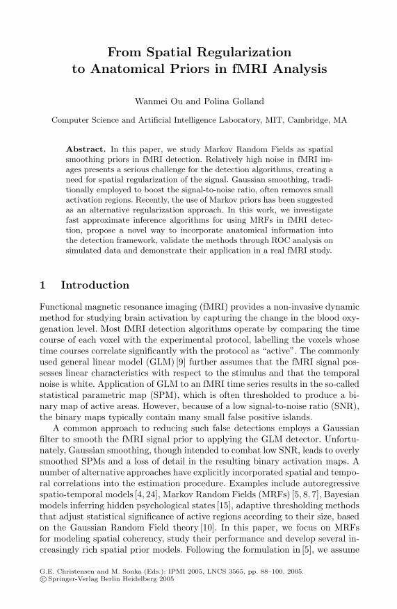
From Spatial Regularizationto Anatomical Priors in fMRI Analysis

Wanmei Ou and Polina Golland

Computer Science and Artificial Intelligence Laboratory, MIT, Cambridge, MA

Abstract. In this paper, we study Markov Random Fields as spatialsmoothing priors in fMRI detection. Relatively high noise in fMRI im-ages presents a serious challenge for the detection algorithms, creating aneed for spatial regularization of the signal. Gaussian smoothing, tradi-tionally employed to boost the signal-to-noise ratio, often removes smallactivation regions. Recently, the use of Markov priors has been suggestedas an alternative regularization approach. In this work, we investigatefast approximate inference algorithms for using MRFs in fMRI detec-tion, propose a novel way to incorporate anatomical information intothe detection framework, validate the methods through ROC analysis onsimulated data and demonstrate their application in a real fMRI study.

1 Introduction

Functional magnetic resonance imaging (fMRI) provides a non-invasive dynamicmethod for studying brain activation by capturing the change in the blood oxy-genation level. Most fMRI detection algorithms operate by comparing the timecourse of each voxel with the experimental protocol, labelling the voxels whosetime courses correlate significantly with the protocol as “active”. The commonlyused general linear model (GLM) [9] further assumes that the fMRI signal pos-sesses linear characteristics with respect to the stimulus and that the temporalnoise is white. Application of GLM to an fMRI time series results in the so-calledstatistical parametric map (SPM), which is often thresholded to produce a bi-nary map of active areas. However, because of a low signal-to-noise ratio (SNR),the binary maps typically contain many small false positive islands.

A common approach to reducing such false detections employs a Gaussianfilter to smooth the fMRI signal prior to applying the GLM detector. Unfortu-nately, Gaussian smoothing, though intended to combat low SNR, leads to overlysmoothed SPMs and a loss of detail in the resulting binary activation maps. Anumber of alternative approaches have explicitly incorporated spatial and tempo-ral correlations into the estimation procedure. Examples include autoregressivespatio-temporal models [4, 24], Markov Random Fields (MRFs) [5, 8, 7], Bayesianmodels inferring hidden psychological states [15], adaptive thresholding methodsthat adjust statistical significance of active regions according to their size, basedon the Gaussian Random Field theory [10]. In this paper, we focus on MRFsfor modeling spatial coherency, study their performance and develop several in-creasingly rich spatial prior models. Following the formulation in [5], we assume

G.E. Christensen and M. Sonka (Eds.): IPMI 2005, LNCS 3565, pp. 88–100, 2005.c© Springer-Verlag Berlin Heidelberg 2005

From Spatial Regularization to Anatomical Priors in fMRI Analysis 89

that, given the activation state of each voxel, the time courses of different voxelsare conditionally independent and can be reduced to a sufficient statistic. Thiswork therefore concentrates on spatial regularization of the activation maps.Temporal regularization models can be easily incorporated into our frameworkby changing the activation statistic.

For MRFs with binary states, exact solution can be obtained in polyno-mial time. An fMRI detection algorithm based on the GLM statistic and thebinary activation states was demonstrated in [5]. However, if one wants to gobeyond binary states (e.g., treating positively and negatively activated voxelsdifferently), the problem of estimating the optimal activation states becomes in-tractable and approximation algorithms must be used. Prior work in MRF-basedfMRI detection employed simulated annealing [8, 21] and the iterated conditionalmode algorithm [22]. We adopt the Mean Field solver, introduced in statisticalphysics [18], which has been widely used for image segmentation [16, 17, 20, 25].In our experiments with binary MRFs, the Mean Field algorithm produced re-sults comparable to those of the exact solver while reducing computation timeby one to two orders of magnitude1.

We further refine the activation priors by incorporating anatomical informa-tion. Similarly to segmentation, where a probabilistic atlas serves as a spatiallyvarying prior on the tissue types, the anatomical information can provide aprior on the activation map. Intuitively speaking, we want the prior to reflectthe fact that activation is much more likely to occur in gray matter than inwhite matter, and not at all in cerebrospinal fluid (CSF) or bone. In addition,the spatial coherency of activation is strong within each tissue and not acrosstissue boundaries. In this model, the hidden nodes encode both the tissue typeand the activation state. Segmentation provides an additional, potentially noisy,observation at each node. We derive the detection algorithm for this model andevaluate it on simulated and real data, achieving high detection accuracy withsignificantly shorter time courses compared to the standard GLM detector.

Anatomical scans have certainly been used in fMRI analysis and visualizationbefore. Hartvig [14] used the anatomical information in his marked point pro-cess spatial prior. Moreover, in some systems (e.g., BrainVoyager [1]), the sub-ject’s anatomical image is transformed into a standard coordinate frame (suchas Talairach) and the functional activation map is displayed on the surface thatcorresponds to the cortical sheet in that coordinate frame. Other systems (e.g.,FSL [2]) rely on sophisticated segmentation algorithms to extract a topologicallycorrect representation of the cortical surface from the anatomical scan [6]. Per-forming Gaussian smoothing on the surface eliminates irrelevant voxels from theweighted average for the cortical locations. In contrast, our approach does notrequire a surface extraction algorithm, but instead utilizes anatomical informa-tion to inject the anatomically based coherency bias into the detection algorithm

1 We also experimented extensively with the Belief Propagation algorithm, which oftenproduces better approximations, but did not find it to be more accurate in thisapplication. We therefore present the results of the Mean Field solution only.

90 W. Ou and P. Golland

while performing the computation directly on the volumetric data. The inspira-tion for this work comes from the success enjoyed by MRFs in providing spatialsmoothing priors for image segmentation [16, 17, 20, 25].

In the next section, we briefly outline how the GLM detector can be aug-mented with an MRF prior closely following the derivation presented in [5], re-view the Mean Field algorithm, and present the empirical evaluation of thedetector on simulated data. In Section 3, we extend the Markov priors to in-corporate the anatomical information and show the empirical evaluation of thisnew, refined model. Section 4 illustrates the proposed detectors on a real fMRIdata set.

2 Markov Priors for Activation Maps

Background. An fMRI scan contains a time course yi ∈ RT for each voxel i

(i = 1, ..., N), where T is the number of time samples and N is the number ofvoxels in the scan. GLM models the fMRI signal as a linear combination of theprotocol-dependent component B, and the protocol-independent component A,such as cardiopulmonary factors. The presence of the protocol-dependent signalindicates that the corresponding voxel is active due to the stimulus. Let H1 bethe hypothesis that a voxel is active and H0 be the null hypothesis. Under GLM,

H0 : yi = Aαi + εi H1 : yi = Aαi + Bβi + εi

for i = 1, ..., N . For white temporal noise, εi ∼ N (0, σ2i I). Least squares esti-

mates of the activation response βi and the protocol-independent factors αi arefound through a linear regression on the design matrix C = [A B]:

[αi βi] = (CTC)−1CTyi, (1)

and the corresponding F-statistic is given by Fi = βTi Σ−1

βiβi/Nβ, where Nβ is the

number of the regression coefficients in βi and Σβiis their estimated covariance.

Let random variable X = [X1, ...,XN ] represent an activation configurationof all voxels in the volume, and x = [x1, ..., xN ] be one possible configuration i.e.,the activation map. In the case of binary hypothesis testing, the random variableXi, which represents the activation state of voxel i, is also binary. Given anfMRI scan [y1, ...,yN ], the GLM estimate of the activation map x∗ is obtainedby thresholding the statistic value Fi for all voxels in the volume at a certainuser-specified level.

It can be shown that the maximum log-likelihood ratio

zi = logmaxαi,βi,σ2

ip(yi|H1)

maxαi,σ2ip(yi|H0)

= logmaxαi,βi,σ2

iN (yi;Bβi + Aαi, σ

2i I)

maxαi,σ2iN (yi;Aαi, σ2

i I)(2)

is a monotonic function of the F statistic (see [5] for a detailed derivation). Wecan therefore consider zi as an alternative statistic indicative of the activationstate of voxel i. We will use this fact in the derivations of the MRF-based de-tection. If a different model of fMRI activation is proposed, it can be easily

From Spatial Regularization to Anatomical Priors in fMRI Analysis 91

incorporated into our algorithm by formulating the corresponding maximumlog-likelihood ratio and using it in place of zi.

Markov Priors. A Markov prior on the activation configuration X, PX(x) =1λ

∏<i,j> Ψij(xi, xj)

∏i Ψi(xi), is defined in terms of the singleton potentials Ψi(xi)

that provide bias over state values xi for voxel i, and the pairwise potentialsΨij(xi, xj) (often referred to as the compatibility matrices) that evaluate thecompatibility of voxel i being in state xi and voxel j being in state xj for eachpair < i, j > of neighboring voxels. λ is a normalization constant, also called thepartition function. Given the activation statistic values z, we seek the maximuma posteriori (MAP) estimate of the activation configuration:

x∗ = arg maxx

PX|Z(x|z) = arg maxx

PX,Z(x,z) = arg maxx

PX(x)PZ|X(z|x)

= arg maxx

1λ

∏<i,j>Ψij(xi, xj)

∏iΨi(xi)PZi|Xi

(zi|xi) (3)

The last equality is based on the assump-

Z4 Z3

Z1 Z2

X4 X3

X1 X2

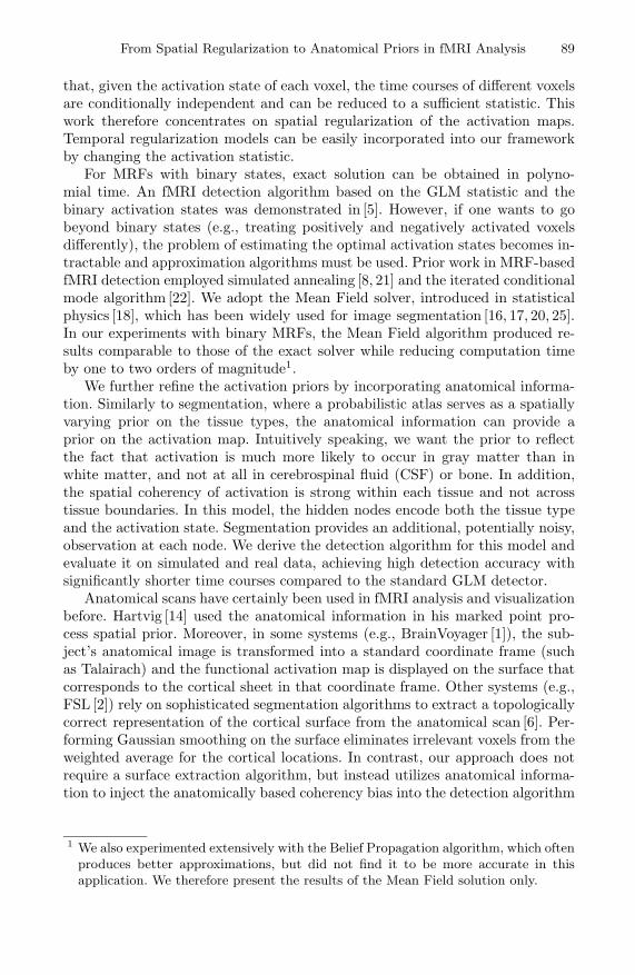
Fig. 1. Graphical model for PX ,Z

tion that the observations at different vox-els are independent given the activationstate of each voxel, and the likelihoodover the volume can therefore be writtenas a product of the individual likelihoodterms for each voxel. Fig. 1 depicts thecorresponding graphical model, using atwo-dimensional grid for illustration pur-poses only. The estimation is performedfully in 3D in all experiment reported here. We assume a spatially stationary gen-erative model, i.e., PZi|Xi

, Ψi, and Ψij are identical for all voxels in the volume.The observations (the fMRI signal, and in Section 3, the anatomical information)move the MAP estimate away from the spatially stationary configurations.

Direct search for the optimal activation configuration is intractable in gen-eral. However, a polynomial-time algorithm for exact MAP estimation exists forbinary MRFs [13], based on a reduction to the Minimum-Cut-Maximum-Flowproblem. We refer to this exact solver as Min-Max throughout this paper. Min-Max is still computationally intensive when applied to the volumetric data: inour experiments, it took 1-3 hours, depending on the pairwise potential settingsand the initial threshold applied to the GLM statistic. On the other hand, theMean Field approximation for MRFs is fast (ten to hundred times faster thanMin-Max on the 3D grids we consider in this paper) and reasonably accurate,as our results in the remainder of this section indicate.

Mean Field Solution. The Mean Field algorithm approximates PX |Z (x|z)

by a product distribution Q(x) =∏

i bi(xi) through minimization of the KL-Divergence between the two distributions:

D(Q||PX|Z) =∑

xQ(x) log(Q(x)) − ∑xQ(x) log(PX|Z(x|z)) (4)

92 W. Ou and P. Golland

bi(xi) denotes the probability of voxel i being in state xi (often called the belief),therefore

∑Mxi=1 bi(xi) = 1, where M is the number of possible states of Xi. The

KL-Divergence measures how closely Q approximates PX |Z ; it is non-negativeand is equal to zero only for Q = PX |Z . It is easy to see that the minimum ofD(·) is achieved for the same state configuration x that minimizes the so calledfree energy, FMF = D(Q||PX |Z )) − log(PZ (z)) − log(λ), since the last two terms ofthe latter function are independent of x. Substituting the product form for Q,we obtain,

FMF (b) = −∑i

∑j∈N (i)

∑Mxi=1

∑Mxj=1bi(xi)bj(xj) log(Ψij(xi, xj))

+∑

i

∑Mxi=1bi(xi)

[log(bi(xi)) − log(PZi|Xi

(zi|xi)Ψi(xi))]

(5)

Setting ∂FMF (b)/∂bi = 0 under the constrains∑M

xi=1 bi(xi) = 1 ∀i yields thefollowing iterative update rule:

bt+1i (xi) ← γ PZi|Xi

(zi|xi) Ψi(xi) e∑

j∈N(i)∑ M

xj=1 btj(xj) log Ψij(xi,xj) (6)

The normalization constant γ ensures the solution is a valid probability distri-bution. N (i) is the set of voxel i’s neighbors. In each iteration of the Mean Fieldalgorithm, the voxel’s belief is updated according to the linear combination of itsneighbors’ beliefs in the previous iteration. The probability model (i.e., PZi|Xi

,Ψi, and Ψij) determines the exact form of the update rule. Each voxel is assignedthe state value with the highest belief at the end of the procedure (for binaryMRFs, the voxel is set active if bi(1) > bi(0)).

Estimating Model Parameters. The potential functions Ψi, and Ψij andthe observation likelihood PZi|Xi

must correspond to our notions of the appro-priate bias toward desired solutions. In this work, we follow a common prac-tice of setting the potential functions (same for all voxels) to the correspondingmarginal probability distributions estimated from data: Ψi(xi) is set to the ex-pected percentage of voxels in state xi, Ψij(xi, xj) is set to the joint frequencyof the states xi and xj , and PZi|Xi

is approximated by a smoother version of aclass-conditional histogram. Other forms of potential functions have also beenexplored [7, 11, 12].

Lack of training data or ground truth necessary for estimating the marginalfrequencies is a more serious problem. Unlike the segmentation application,where manual segmentations by experts can be used to construct priors onthe frequencies and co-occurrences of tissue types, in most fMRI experimentseven the experts cannot provide such information. Model parameters in the cur-rently used detectors are either set using researcher’s intuition on the underlyingactivation properties (e.g., the threshold in GLM or the kernel width in Gaus-sian smoothing) or estimated from the input images (e.g., the noise variance inGLM). We take a similar approach of first running the GLM detector withoutsmoothing and using the resulting SPM at a user-chosen threshold to estimatethe probability model. To study the sensitivity of the method to the parameter

From Spatial Regularization to Anatomical Priors in fMRI Analysis 93

SNR = -9dB SNR = -6dB

1e−05 0.0001 0.001 0.01 0.1 10

0.1

0.2

0.3

0.4

0.5

0.6

0.7

0.8

0.9

1

False Positive

Tru

e P

ositi

ve

No SmoothingGaussianMRFMin−Max

1e−05 0.0001 0.001 0.01 0.1 10

0.1

0.2

0.3

0.4

0.5

0.6

0.7

0.8

0.9

1

False Positive

Tru

e P

ositi

ve

No SmoothingGaussianMRFMin−Max

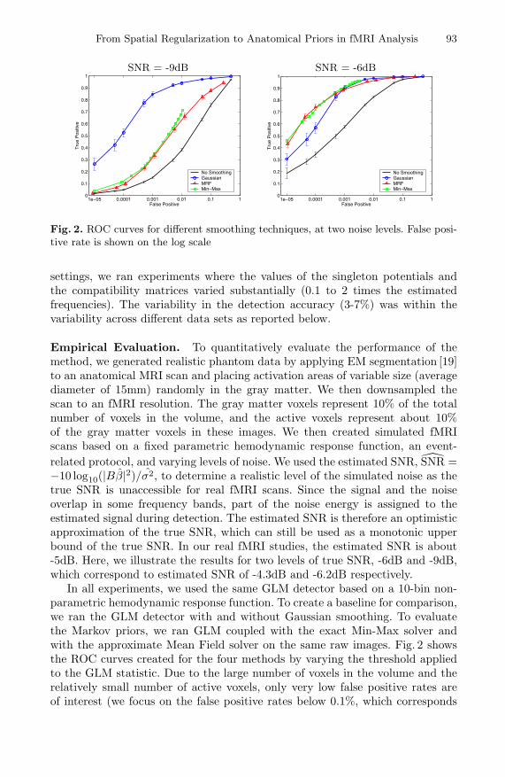
Fig. 2. ROC curves for different smoothing techniques, at two noise levels. False posi-tive rate is shown on the log scale

settings, we ran experiments where the values of the singleton potentials andthe compatibility matrices varied substantially (0.1 to 2 times the estimatedfrequencies). The variability in the detection accuracy (3-7%) was within thevariability across different data sets as reported below.

Empirical Evaluation. To quantitatively evaluate the performance of themethod, we generated realistic phantom data by applying EM segmentation [19]to an anatomical MRI scan and placing activation areas of variable size (averagediameter of 15mm) randomly in the gray matter. We then downsampled thescan to an fMRI resolution. The gray matter voxels represent 10% of the totalnumber of voxels in the volume, and the active voxels represent about 10%of the gray matter voxels in these images. We then created simulated fMRIscans based on a fixed parametric hemodynamic response function, an event-related protocol, and varying levels of noise. We used the estimated SNR, SNR =−10 log10(|Bβ|2)/σ2, to determine a realistic level of the simulated noise as thetrue SNR is unaccessible for real fMRI scans. Since the signal and the noiseoverlap in some frequency bands, part of the noise energy is assigned to theestimated signal during detection. The estimated SNR is therefore an optimisticapproximation of the true SNR, which can still be used as a monotonic upperbound of the true SNR. In our real fMRI studies, the estimated SNR is about-5dB. Here, we illustrate the results for two levels of true SNR, -6dB and -9dB,which correspond to estimated SNR of -4.3dB and -6.2dB respectively.

In all experiments, we used the same GLM detector based on a 10-bin non-parametric hemodynamic response function. To create a baseline for comparison,we ran the GLM detector with and without Gaussian smoothing. To evaluatethe Markov priors, we ran GLM coupled with the exact Min-Max solver andwith the approximate Mean Field solver on the same raw images. Fig. 2 showsthe ROC curves created for the four methods by varying the threshold appliedto the GLM statistic. Due to the large number of voxels in the volume and therelatively small number of active voxels, only very low false positive rates areof interest (we focus on the false positive rates below 0.1%, which corresponds

94 W. Ou and P. Golland

to about 10% of the total number of the active voxels, or approximately 250voxels). The error bars indicate the standard deviation of the true detection rateover 15 different, independently created and processed, data sets. The Min-MaxROC curve does not have the error bars, as the estimation takes too long (1to 3 hours for a single run). Moreover, the Min-Max ROC curve is incompletebecause extreme threshold values cause it to run even longer (we stopped theruns after 3 hours).

The Mean Field detection accuracy is very close to the exact Min-Max solu-tion, providing a reasonable approximation to the exact solution that also takesmuch less time to compute (most Mean Field runs finished in a few minutes).The Min-Max accuracy is sometimes lower than the Mean Field accuracy, whichappears to contradict the optimality of Min-Max. However, we note that bothalgorithms solve a particular estimation problem that does not necessarily de-scribe the ground truth precisely but rather approximates it using a Markovmodel. Thus, the lowest energy state under this model might not be the bestdetector in practice. It is still reassuring to see that the approximate solver per-forms as well as the exact algorithm. It also suggests that more realistic spatialpriors could further improve the detection accuracy.

As expected, the accuracy of all methods improves with increasing SNR. Athigh noise levels (low SNR), Gaussian smoothing outperforms MRFs. As thesimplest smoothing technique, Gaussian smoothing is more robust to noise. Wealso believe that our current way of constructing the likelihood term in theMRF model over-emphasizes the data evidence over the prior. We are inves-tigating ways to compensate for this in the estimation of the model. As theSNR increases, MRFs provide better regularization of the activation state (forexample, at SNR=-6dB, at the false positive rate of 0.01%, the MRF outper-forms the Gaussian smoothing by about 15% in true detection accuracy; at 70%true detection, the MRF approximately halves the false detections compared tothe Gaussian smoothing). With the improving scanning technology, we believeMRFs will become even more helpful in reducing spurious false detection islands.

3 Anatomical Priors for Spatial Regularization

The general nature of the Mean FieldZ1 Z2

W1 W2

Z4

W3

Z3

U4 U3

U1 U2

W4

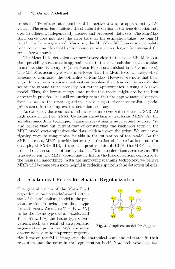
Fig. 3. Graphical model for PU ,Z ,W

algorithm allows straightforward exten-sion of the probabilistic model in the pre-vious section to include the tissue typefor each voxel. We define V = [V1, ..., VN ]

to be the tissue types of all voxels, andW = [W1, ..., WN ] the tissue type obser-vations, such as a result of an automaticsegmentation procedure. Wi’s are noisyobservations due to imperfect registra-tion between the fMRI image and the anatomical scan, the mismatch in theirresolution and the noise in the segmentation itself. Now each voxel has two

From Spatial Regularization to Anatomical Priors in fMRI Analysis 95

hidden attributes: the activation state Xi and the tissue type Vi. We combinethese attributes into a single hidden node Ui, as illustrated in Fig. 3. For exam-ple, for a binary activation states (active or not active) and three tissue types(gray matter, white matter, or other), Ui has six possible states. Similarly to thederivations in the previous section, the MAP estimate in this case is as follows:

u∗ = arg maxu

PU |Z,W (u|z,w) = arg maxu

PU (u)PZ|U (z|u)PW |U (w|u)

= arg maxu

1λ

∏<i,j>Ψij(ui, uj)

∏iΨi(ui)PZi|Ui

(zi|ui)PWi|Ui(wi|ui) (7)

We assume that the segmentation W and the fMRI observation Z are condi-tionally independent given the state of the voxel since they are obtained fromtwo different images. Similarly to the previous section, we derive the iterativeupdate step in the estimation procedure:

bt+1i (ui) ← γPWi|Ui

(wi|ui)PZi|Ui(zi|ui)Ψi(ui)e

∑j∈N(i)

∑ Muj=1 bt

j(uj) log Ψij(ui,uj)

(8)This update rule is similar to Eq. (6), with the exception of the extra likelihoodterm PWi|Ui

(wi|ui) for the tissue type observation. The compatibility matrixΨij(xi, xj) is M × M , where M is the number of states in Ui.

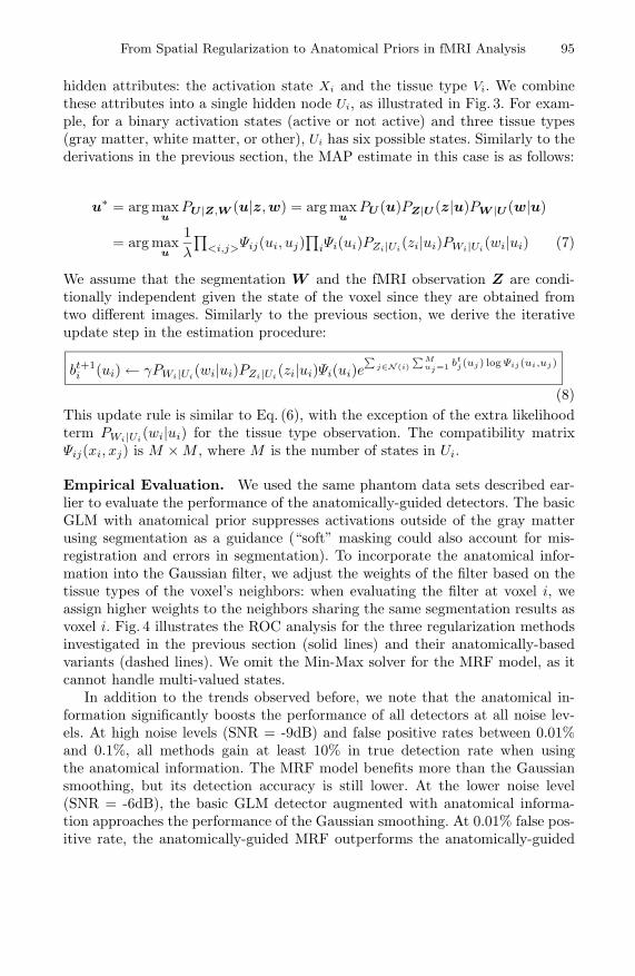
Empirical Evaluation. We used the same phantom data sets described ear-lier to evaluate the performance of the anatomically-guided detectors. The basicGLM with anatomical prior suppresses activations outside of the gray matterusing segmentation as a guidance (“soft” masking could also account for mis-registration and errors in segmentation). To incorporate the anatomical infor-mation into the Gaussian filter, we adjust the weights of the filter based on thetissue types of the voxel’s neighbors: when evaluating the filter at voxel i, weassign higher weights to the neighbors sharing the same segmentation results asvoxel i. Fig. 4 illustrates the ROC analysis for the three regularization methodsinvestigated in the previous section (solid lines) and their anatomically-basedvariants (dashed lines). We omit the Min-Max solver for the MRF model, as itcannot handle multi-valued states.

In addition to the trends observed before, we note that the anatomical in-formation significantly boosts the performance of all detectors at all noise lev-els. At high noise levels (SNR = -9dB) and false positive rates between 0.01%and 0.1%, all methods gain at least 10% in true detection rate when usingthe anatomical information. The MRF model benefits more than the Gaussiansmoothing, but its detection accuracy is still lower. At the lower noise level(SNR = -6dB), the basic GLM detector augmented with anatomical informa-tion approaches the performance of the Gaussian smoothing. At 0.01% false pos-itive rate, the anatomically-guided MRF outperforms the anatomically-guided

96 W. Ou and P. Golland

SNR = -9dB SNR =-6dB

1e−05 0.0001 0.001 0.01 0.1 10

0.1

0.2

0.3

0.4

0.5

0.6

0.7

0.8

0.9

1

False Positive

True

Pos

itive

No SmoothingNo Smoothing+AnaGaussianGaussian+AnaMRFMRF+Ana

1e−05 0.0001 0.001 0.01 0.1 10

0.1

0.2

0.3

0.4

0.5

0.6

0.7

0.8

0.9

1

False Positive

True

Pos

itive

No SmoothingNo Smoothing+AnaGaussianGaussian+AnaMRFMRF+Ana

Fig. 4. ROC curves for different smoothing techniques augmented with the anatomicalinformation, at two noise levels. False positive rate is shown on the log scale

Gaussian smoothing by about 15% in true detection rate, achieving over 90%detection accuracy. The large boost experienced by the basic GLM when aug-mented with anatomical information is easy to understand: since false detectionsoccur relatively uniformly throughout the volume, masking the gray matter im-proves the performance substantially.

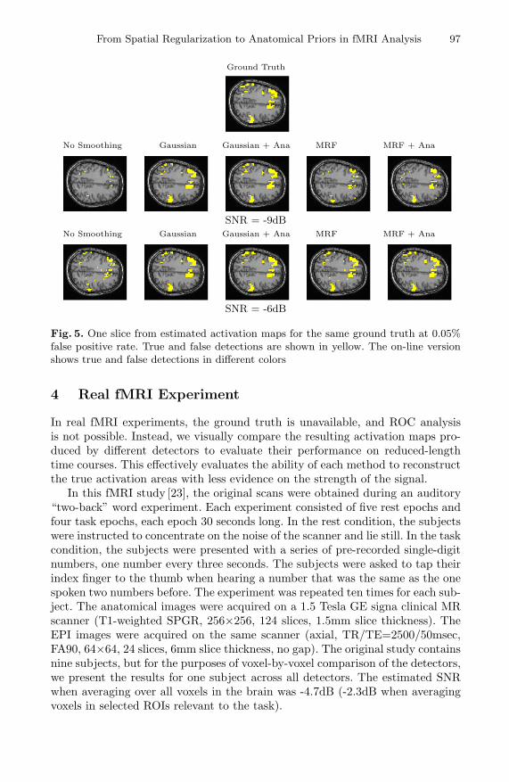
In addition to the quantitative analysis presented above, we find it usefulto visually inspect the resulting activation maps. Fig. 5 illustrates the detec-tion results by showing one axial slice of the estimated activation map. Thetop image shows the phantom activation areas that were placed in the volumeand used to generate the simulated fMRI scan. The middle and the bottomrows show the same slice in the reconstructed volume at two different noiselevels. All the reconstructions were performed at 0.05% false positive rate. Inother words, each image in Fig. 5 shows one slice in the reconstructed volumethat corresponds to a point on the ROC curve of the respective detector at0.05% false positive rate.

The basic GLM produces a fragmented activation map that contains a num-ber of false detection islands at high SNR and shows very little of the originalactivation at low SNR. Given either of these maps, the users would have troublesinferring the true activation areas and disambiguating them from spurious falsedetections. The Gaussian smoothing leads to a reasonable estimate of the groundtruth. Gaussian smoothing tends to make the detections “spherical”, which maychange the shape of the detected activations. The smoothing effectively over-estimates the extent of the regions. Consequently, many false positive voxelsin the Gaussian smoothing occur at the boundaries of the activation regions.Imposing anatomical information reduces this over-smoothing effect for some ofthe areas. At low SNR (-9dB), the MRF model fills in many of the active pixelsthat were missed by the GLM, but as we saw before, it does not produce asaccurate result as Gaussian smoothing. At higher SNR (-6dB), MRF producesa relatively accurate result. Not all of the scatter activation islands are removedthrough regularization, but the activation map looks more similar to the groundtruth. The activation map is further improved when the anatomical informationis incorporated into the model.

From Spatial Regularization to Anatomical Priors in fMRI Analysis 97

Ground Truth

No Smoothing Gaussian Gaussian + Ana MRF MRF + Ana

SNR = -9dBNo Smoothing Gaussian Gaussian + Ana MRF MRF + Ana

SNR = -6dB

Fig. 5. One slice from estimated activation maps for the same ground truth at 0.05%false positive rate. True and false detections are shown in yellow. The on-line versionshows true and false detections in different colors

4 Real fMRI Experiment

In real fMRI experiments, the ground truth is unavailable, and ROC analysisis not possible. Instead, we visually compare the resulting activation maps pro-duced by different detectors to evaluate their performance on reduced-lengthtime courses. This effectively evaluates the ability of each method to reconstructthe true activation areas with less evidence on the strength of the signal.

In this fMRI study [23], the original scans were obtained during an auditory“two-back” word experiment. Each experiment consisted of five rest epochs andfour task epochs, each epoch 30 seconds long. In the rest condition, the subjectswere instructed to concentrate on the noise of the scanner and lie still. In the taskcondition, the subjects were presented with a series of pre-recorded single-digitnumbers, one number every three seconds. The subjects were asked to tap theirindex finger to the thumb when hearing a number that was the same as the onespoken two numbers before. The experiment was repeated ten times for each sub-ject. The anatomical images were acquired on a 1.5 Tesla GE signa clinical MRscanner (T1-weighted SPGR, 256×256, 124 slices, 1.5mm slice thickness). TheEPI images were acquired on the same scanner (axial, TR/TE=2500/50msec,FA90, 64×64, 24 slices, 6mm slice thickness, no gap). The original study containsnine subjects, but for the purposes of voxel-by-voxel comparison of the detectors,we present the results for one subject across all detectors. The estimated SNRwhen averaging over all voxels in the brain was -4.7dB (-2.3dB when averagingvoxels in selected ROIs relevant to the task).

98 W. Ou and P. Golland

(a) No smoothing (long) (c) Gaussian (e) MRF

(b) No smoothing (d) Gaussian + Ana (f) MRF + Ana

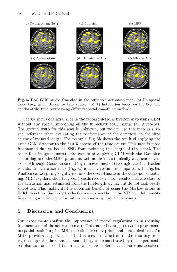
Fig. 6. Real fMRI study. One slice in the estimated activation map. (a) No spatialsmoothing, using the entire time course. (b)-(f) Estimation based on the first fiveepochs of the time course using different spatial smoothing methods

Fig. 6a shows one axial slice in the reconstructed activation map using GLMwithout any spatial smoothing on the full-length fMRI signal (all 9 epochs).The ground truth for this scan is unknown, but we can use this map as a vi-sual reference when evaluating the performance of the detectors on the timecourse of reduced length. For example, Fig. 6b shows the result of applying thesame GLM detector to the first 5 epochs of the time course. This map is morefragmented due to loss in SNR from reducing the length of the signal. Theother four images illustrate the results of applying GLM with the Gaussiansmoothing and the MRF priors, as well as their anatomically augmented ver-sions. Although Gaussian smoothing removes most of the single voxel activationislands, its activation map (Fig. 6c) is an overestimate compared with Fig. 6a.Anatomical weighting slightly reduces the overestimate in the Gaussian smooth-ing. MRF regularization (Fig. 6e,f) yields reconstruction results that are close tothe activation map estimated from the full-length signal, but do not look overlysmoothed. This highlights the potential benefit of using the Markov priors infMRI detection. Similarly to the Gaussian smoothing, the MRF model benefitsfrom using anatomical information to remove spurious activations.

5 Discussion and Conclusions

Our experiments confirm the importance of spatial regularization in reducingfragmentation of the activation maps. This paper investigates two improvementsin spatial modelling for fMRI detection: Markov priors and anatomical bias. AnMRF provides a spatial prior that refines the structure of the resulting acti-vation map over the Gaussian smoothing, as demonstrated by our experimentson phantom and real data. In this work, we explored fast approximate solvers

From Spatial Regularization to Anatomical Priors in fMRI Analysis 99

in application to MRF-based fMRI detection and showed that they provide rea-sonably accurate approximations to the exact solution while taking substantiallyless time to evaluate. We also note that since the Markov model itself is an ap-proximation of the real geometry of the activation regions, we should not dwellon the small differences in the activation maps introduced by the approximatesolvers but rather focus on their performance relative to the ground truth.

A separate insight of this paper is that we can use anatomical information tobias the fMRI detector. Gaussian smoothing can be straightforwardly augmentedwith the anatomical prior by rescaling the coefficients of the smoothing kernel.Moreover, we derived an algorithm for anatomically-guided MRF estimation.One of the problems that should be investigated in the future is the partialvoluming effects. The anatomical information comes at much higher resolutionthan the fMRI signals. Right now, we downsample the anatomical scan to matchthe resolution of the functional scan. A better solution would be to use the high-resolution anatomical scans to resolve the activation in the functional voxels thatare on the boundary of the gray matter, leading to a “super-resolution” detector.

We evaluated the methods on phantom data by performing ROC analysisand on real data by studying their ability to recover activation from signifi-cantly shorter time courses. While in high noise settings the Gaussian smoothingoutperformed other methods, as the SNR in the images increased, the Markovpriors offered a substantial improvement in the detection accuracy. Using thissmoothing prior enabled us to shorten fMRI scan length by half while retainingthe detection power comparable with the full-length fMRI scan. We expect asimilar effect to occur with respect to the spatial resolution when we extend themethod to utilize the anatomical information at the original scan resolution. Asthe quality of the scanning equipment improves, the sophisticated spatial mod-els, such as MRFs, will become even more important in recovering the details ofthe activation regions.

Acknowledgement. We thank Sandy Wells for suggesting we look at the MRFregularization for fMRI applications, Eric Cosman and Kilian Pohl for help onthis paper, and Dr. L.P. Panych for providing fMRI data. This work was partiallysupported by the NIH National Center for Biomedical Computing Program,National Alliance for Medical Imaging Computing (NAMIC), Fund No. 1U54EB005149, the NSF IIS 9610249 grant. fMRI acquisition was supported by theNIH R01 NS37922 grant.

References

1. BrainVoyager software package. http://www.brainvoyager.de.2. FMRIB software library. http://www.fmrib.ox.ac.uk/fsl.3. Besag, J. Spatial interaction and statistical analysis of lattice systems.

Acad. R. Statistical Soc. Series B, 36:721–741, 1974.4. Burock, M.A., and Dale, A.M. Estimation and detection of event-related fmri

signals with temporally correlated noise: A statistically efficient and unbiased ap-proach. Human Brain Mapping, 11:249–260, 2000.

100 W. Ou and P. Golland

5. Cosman, E.R., Fisher, J. and Wells, W.M. Exact MAP activity detection in fMRIusing a GLM with an spatial. In Proc. MICCAI’04, 2:703–710, 2004.

6. A. M. Dale, et al. Cortical Surface-Based Analysis I: Segmentation and SurfaceReconstruction. NeuroImage, 9:179-194, 1999.

7. Descombes, X., Kruggel, F., and Von Cramon, D.Y. fMRI signal restoration usinga spatio-temporal Markov random field preserving transitions. NeuroImage, 8:340–349, 1998.

8. Descombes, X., Kruggel, F. and Von Cramon, D.Y. Spatio-temporal fMRI analysisusing Markov random fields. IEEE TMI, 17(6):1028–1039, 1998.

9. Friston, K.J., et al. Statistical parametric maps in functional imaging: a generallinear approach. Human Brain Mapping, 2:189–210, 1995.

10. Friston, K.J., et al. Assessing the significance of local activations using their spatialextent. Human Brain Mapping, 1:210–220, 1994.

11. Geman, S. and McClure, D. Statistical methods for tomographic image reconstruc-tion. Proc. 46th Session of ISI, 51:22–26, 1987.

12. Geman, S. and Reynolds, G. Constrained restoration and recovery of discontinu-ities. IEEE Trans. PAMI, 14:367–383, 1992.

13. Greig, D.M., Porteous, B.T. and Gramon, D.Y. Exact maximum a posterioriestimation for binary images. J. R. Statistical Society, 51:271–279, 1989.

14. Hartvig, N.V. A stochastic Geometry model for functional Magnetic resonanceimages Scandinavian Journal of Statistics, 29:333–253, 2002.

15. Hojen-Sorensen, F., Hansen, L.K. and Rasmussen, C.E. Bayesian modeling of fMRItime series. Adv. Neuroinform. Processing Syst., Vol.12:754–760, 2000.

16. Kapur, T., et al. Enhanced spatial priors for segmentation of magnetic resonanceimagery. Proc. MICCAI’98, 148-157, 1998.

17. Langan, D.A., et al. Use of the mean-field approximation in an EM-based approachto unsupervised stochastic model-based image segmentation. Proc. ICASSP, 3:57–60, 1992.

18. G. Parisi. Statistical Field Theory. Addison-Wesley, 1998.19. Pohl, K.M., et al. Anatomical guided segmentation with non-stationary tissue class

distributions in an expectation-maximization framework. Proc. IEEE ISBI, 81–84,2004.

20. Pohl, K.M., et al. Incorporating non-rigid registration into expectation maximiza-tion algorithm to segment MR images. Proc. MICCAI’02, 508-515, 2002.

21. Rajapakse, J.C. and Piyaratna, J. Bayesian modeling of fMRI time series. IEEETransactions on Biomedical Engineering, 48:1186–1194, 2001.

22. Salli, E., et al. Contextual clustering for analysis of functional MRI data. IEEETMI, 20:403–413, 2001.

23. Wei, X., et al. Functional MRI of auditory verbal working memory: long-termreproducibility analysis. NeuroImage, 21:1000-1008, 2004.

24. Woolrich, M.W., et al. Fully Bayesian spatio-temporal modeling of fMRI data.IEEE TMI, 23(2):213–231, 2004.

25. Zhang, J. The mean-field theory in EM procedures for markov random field. IEEETrans. on Signal Processing, 40:2570–2583, 1992.