FROM THE BIRCH AND SWINNERTON-DYER CONJECTURE TONAGAO’S CONJECTURE

SEOYOUNG KIM AND M. RAM MURTYWITH AN APPENDIX BY ANDREW V. SUTHERLAND

Abstract. Let E be an elliptic curve over Q with discriminant ∆E . For primes p of goodreduction, let Np be the number of points modulo p and write Np = p+1−ap. In 1965, Birchand Swinnerton-Dyer formulated a conjecture which implies

limx→∞

1

logx∑p≤x

p∤∆E

ap log p

p= −r + 1

2,

where r is the order of the zero of the L-function LE(s) of E at s = 1, which is predictedto be the Mordell-Weil rank of E(Q). We show that if the above limit exits, then the limitequals −r + 1/2. We also relate this to Nagao’s conjecture.

1. Introduction

Let E be an elliptic curve over Q with discriminant ∆E and conductor NE. For each primep ∤∆E, we write the number of points of E (mod p) as

Np ∶= #E(Fp) = p + 1 − ap, (1.1)

where ap satisfies Hasse’s inequality ∣ap∣ ≤ 2√p. For p ∣ ∆E, we define ap = 0,−1, or 1 ac-

cording as E has additive reduction, split multiplicative reduction, or non-split multiplicativereduction at p (For precise definitions of this terminology, we refer the reader to [14, p. 449]).

The L-function attached to E, denoted as LE(s) is then defined as an Euler product usingthis datum:

LE(s) = ∏p∣∆E

(1 −apps

)−1

∏p∤∆E

(1 −apps

+ p

p2s)−1

, (1.2)

which converges absolutely for Re(s) > 3/2 by virtue of Hasse’s inequality. Expanding theEuler product into a Dirichlet series, we write

LE(s) =∞∑n=1

anns. (1.3)

If we write αp, βp as the eigenvalues of the Frobenius morphism at p, for p ∤ ∆E, we canwrite ap = αp + βp, and our L-function can be re-written as

LE(s) = ∏p∣∆E

(1 −apps

)−1

∏p∤∆E

(1 −αpps

)−1

(1 −βpps

)−1

, (1.4)

Date: June 3, 2021.Research of the first author partially supported by a Coleman Postdoctoral Fellowship.Research of the second author partially supported by NSERC Discovery grant.

1

arX

iv:2

105.

1080

5v3

[m

ath.

NT

] 1

Jun

202

1

and by Hasse’s inequality ∣αp∣ = ∣βp∣ =√p.

By the elliptic modularity theorem for semistable elliptic curves over Q by Wiles [19], andits complete extension to all elliptic curves over Q by Breuil, Conrad, Diamond, and Taylor[1], LE(s) extends to an entire function and satisfies a functional equation which relatesLE(s) to LE(2 − s). More precisely, if we define

ΛE(s) = N s/2E (2π)−sΓ(s)LE(s), (1.5)

then ΛE(s) is entire and satisfies the following functional equation:

ΛE(s) = wEΛE(2 − s), (1.6)

where wE ∈ {1,−1} is the root number of E. Since Γ(s) has simple poles at s = 0,−1, . . .,LE(s) has trivial zeros at s = 0,−1, . . .. Thus, for m = 0,1,2,⋯, we have

Ress=−m

L′E(s)LE(s)

= Ress=−m

[Λ′E(s)

ΛE(s)− Γ′(s)

Γ(s)] . (1.7)

This summarises our study of E from the analytic perspective.

From the algebraic perspective, a celebrated theorem of Mordell states that the group ofrational points E(Q) is a finitely generated abelian group with rank rM . In 1965, Birch andSwinnerton-Dyer [2] conjectured that LE(s) has a zero of order r at s = 1. In other words,the algebraic rank rM equals the “analytic rank” reflected as the order of zero at s = 1 ofLE(s). This conjecture is often referred to as the Birch and Swinnerton-Dyer conjecture.

However, before they formulated this conjecture in this form, Birch and Swinnerton-Dyerstated a stronger conjecture motivated by a heuristic “local-global” principle: the rank shouldbe reflected by “modulo p” information for many primes p. More precisely, they conjecturedthat there is a constant CE such that

∏p<xp∤∆E

Np

p∼ CE(logx)r, (1.8)

as x→∞. We refer to this as the original Birch and Swinnerton-Dyer conjecture (or OBSDfor short).

Several authors have noted that the “severity” of this conjecture in that it implies theanalog of the Riemann hypothesis for LE(s), and much more. This was first announced byGoldfeld [7]. Kuo and Murty [8, Theorem 2, Theorem 3], and K. Conrad [3, Theorem 1.3]independently noticed that (1.8) goes well beyond the analog of the Riemann hypothesis forLE(s). They proved that (1.8) is true if and only if

∑pk≤xp∤∆E

αkp + βkpk

= o(x), (1.9)

as x→∞, or equivalently

∑pk≤xp∤∆E

(αkp + βkp) log p = o(x logx), (1.10)

2

as x→∞, whereas, the Riemann hypothesis for LE(s) is equivalent to the weaker assertion

∑pk≤xp∤∆E

(αkp + βkp) log p = O(x(logx)2), (1.11)

as x→∞.

If we return to the heuristic “local-global” principle that perhaps motivated Birch andSwinnerton-Dyer to make their OBSD conjecture, we are led to formulate several gradationsof their conjecture.

The first is that (1.8) is equivalent to

∑pk≤xp∤∆E

αkp + βkpkpk

= −r log logx +A + o(1), (1.12)

for some constant A, as x → ∞. If we weight each prime power pk by log p (followingChebysheff), we have that (1.8) implies

∑pk≤xp∤∆E

αkp + βkpkpk

log p = −r logx +O(1), (1.13)

as x→∞. In fact, this is equivalent to (1.8). However, the weaker assertion

∑pk≤xp∤∆E

αkp + βkpkpk

log p = −r logx + o(logx) (1.14)

already implies the analog of the Riemann hypothesis for LE(s) and still leads to an analyticdetermination of the rank r using the “local” data ap.

There are good reasons to believe that (1.11) is not the optimal estimate. Montgomery[10] and Gallagher [6] have suggested in the context of the Riemann zeta function (but hereapplied to our context) that the error in (1.11) should be

O(x(log log logx)2) (1.15)

or even the “weaker” O(x(log logx)2).

In either cases, it is conceivable that OBSD is true, even though it goes well beyond theanalog of the Riemann hypothesis for LE(s).

The purpose of this note is to show that if the limit

limx→∞

1

logx∑pk≤xp∤∆E

αkp + βkpkpk

log p (1.16)

exists, then the limit is −r. Moreover, this implies that if the limit

limx→∞

1

logx∑p<x

ap log p

p(1.17)

3

exists, then the Riemann hypothesis for LE(s) is true, and the limit is −r + 1/2. We applya technique of Cramer [4] to prove our theorem.

2. Preliminaries

For an elliptic curve E defined over Q with discriminant ∆E and conductor NE, we definedits L-function LE(s) in (1.2). Hence, we can write its logarithmic derivative as

−L′E(s)LE(s)

=∞∑n=1

cnΛ(n)ns

, (2.1)

where Λ(n) is the von Mangoldt function, and

cn =⎧⎪⎪⎪⎨⎪⎪⎪⎩

αmp + βmp , if n = pm and p ∤ N ,amp , if n = pm and p ∣ N ,0, otherwise.

(2.2)

Let C be the (oriented) rectangle with vertices c−iR, c+iR,−U+iR,−U−iR, and its edges aredenoted by I1, I2, I3, and I4 respectively, with c = 2, an odd positive integer R (R is chosenso that it is not the ordinate of a zero of LE(s)), and U a positive non-integral number, wehave by the Cauchy residue theorem,

1

2πi ∫C−L′E(s)LE(s)

xs

sds = −∑

∣γ∣<Rnρxρ

ρ− ∑m<U

Ress=−m

[L′E(s)LE(s)

xs

s] , (2.3)

where the sum is over all zeros ρ = β + iγ of LE(s), and nρ is the multiplicity of each ρ. Forany n ≥ 1, Hence, by (truncated) Perron’s formula, for x not an integer, we get

∑n≤x

cnΛ(n) = 1

2πi ∫2+iR

2−iR−L′E(s)LE(s)

xs

sds +O (

∞∑n=1

(xn)

2

∣cnΛ(n)∣ ⋅min(1,1

R∣ log xn ∣

)) (2.4)

= −∑∣γ∣<R

nρxρ

ρ− ∑m<U

Ress=−m

[L′E(s)LE(s)

xs

s] + 1

2πi ∫C/I1L′E(s)LE(s)

xs

sds (2.5)

+O (∞∑n=1

(xn)

2

∣cnΛ(n)∣ ⋅min(1,1

R∣ log xn ∣

)) , (2.6)

= −∑∣γ∣<R

nρxρ

ρ+ ∑m<U

x−m

m+ 1

2πi ∫C/I1L′E(s)LE(s)

xs

sds +E(x,U,R), (2.7)

where the first sum is over all nontrivial zeros ρ = 1 + iγ of LE(s), and nρ is the multiplicityof each ρ. E(x,U,R) is the error term arising from the last term in (2.6). We first estimatethe error term in (2.6) and (2.7):

E(x,U,R) = O (∞∑n=1

(xn)

2

∣cnΛ(n)∣ ⋅min(1,1

R∣ log xn ∣

)) .

We consider the following three parts of the sum in E(x,U,R) separately:

⎛⎝ ∑n<x/2

+ ∑x/2<n<2x

+ ∑n>2x

⎞⎠(xn)

2

∣cnΛ(n)∣ ⋅min(1,1

R∣ log xn ∣

) . (2.8)

4

The first sum is for n < x/2, and hence we have log(x/n) > log 2, and

∑n<x/2

(xn)

2

∣cnΛ(n)∣ ⋅min(1,1

R∣ log xn ∣

) = O⎛⎝x2

R∑n<x/2

∣cnΛ(n)∣n2

⎞⎠= O (x

2

R) , (2.9)

for big enough R. Similarly, for the third sum of (2.8), the condition n > 2x implies∣ log(x/n)∣ > log 2, and hence

∑n>2x

(xn)

2

∣cnΛ(n)∣ ⋅min(1,1

R∣ log xn ∣

) = O (x2

R) . (2.10)

Now, it remains to compute the second sum of (2.8)

∑x/2<n<2x

(xn)

2

∣cnΛ(n)∣ ⋅min(1,1

R∣ log xn ∣

) .

We observe that x/2 < n < 2x implies

−2 < −xn< x − n

n< x

2n< 1,

and therefore

∑x/2<n<2x

(xn)

2

∣cnΛ(n)∣ ⋅min(1,1

R∣ log xn ∣

) = O⎛⎝ ∑x/2<n<2x

∣cnΛ(n)∣ ⋅ n

R∣x − n∣⎞⎠. (2.11)

We choose x = N + 1/2, an integer plus half, then x − n ranges

−N − 1

2< x − n < 0,

and thus, by denoting j = ∣x − n∣, the sum can be rewritten by

∑x<n<2x

1

∣x − n∣=

2N+1

∑j=1

1

j/2=≤ log(2N + 1). (2.12)

One can similarly treat the range x/2 < n < x to deduce

∑x/2<n<2x

(xn)

2

∣cnΛ(n)∣ ⋅min(1,1

R∣ log xn ∣

) = O (2x√x(logx)2

R) . (2.13)

In conclusion, we obtain from (2.9), (2.10), and (2.13),

E(x,U,R) = O (x2

R) ,

for suitable choice of x. The third term in (2.7)

1

2πi ∫C/I1L′E(s)LE(s)

xs

sds

can be estimated with the usual method. We consider the following part of the sum fromprimes of good reduction:

ψE(t) =∑n≤tcnΛ(n), (2.14)

and similar to the estimation of Cramer [4], we have the following result:5

Theorem 1. Assuming the Riemann hypothesis for LE(s) is true, we obtain

limx→∞

1

logx ∫x

2

ψ2E(t)t3

dt =∑ρ

∣nρρ

∣2

, (2.15)

where the sum is over all nontrivial zeros ρ of LE(s), and nρ is the multiplicity of each ρ.

Proof. From (2.8), and following estimations, we have

ψ2E(t)t3

= 1

t3(∑ρ

nρtρ

ρ+O (t

2

R))

2

=∑ρ

nρ∑ρ′nρ′

tρ+ρ′−3

ρρ′+O ( t

R2) +O ( 1

R∣∑ρ

nρtρ−1

ρ∣)

=∑ρ

nρ∑ρ′nρ′

tρ+ρ′−3

ρρ′+O ( t

R2) +O (t

3/2(log t)2

R) ,

where the sums involving ρ and ρ′ are taken over the zeros of LE(s) satisfying ∣ Im(ρ)∣ < Rand ∣ Im(ρ′)∣ < R (For simplifying the notation, we will drop these constraints throughoutthe proof), we assume the same condition for such sums throughout the proof. Thus, usingthe relation ρ(2 − ρ) = ∣ρ∣2 and ρ = 2 − ρ, and by choosing large enough R in (2.7), we obtain

∫x

2

ψ2E(t)t3

dt =∑ρ

nρρ∑ρ′

nρ′

ρ′ ∫x

2tρ+ρ

′−3dt +O(1)

=∑ρ

nρρ

[ ∑ρ′=2−ρ

nρ′

ρ′ ∫x

2tρ+ρ

′−3dt + ∑ρ′≠2−ρ

nρ′

ρ′ ∫x

2tρ+ρ

′−3dt] +O(1)

= logx∑ρ

∣nρρ

∣2

+∑ρ

nρρ∑

ρ′≠2−ρ

nρ′

ρ′⋅ x

ρ+ρ′−2 − 2ρ+ρ′−2

ρ + ρ′ − 2+O(1).

Note that ρ′ = 2−ρ implies Im(ρ′) = − Im(ρ). We are now going to estimate the second term

∑ρ

nρρ∑

ρ′≠2−ρ

nρ′

ρ′⋅ x

ρ+ρ′−2 − 2ρ+ρ′−2

ρ + ρ′ − 2.

Let η > 0 be sufficiently small, which is independent from x, so that it is smaller than thesmallest positive γ. We will estimate the sum separately for two different cases:

∣ρ + ρ′ − 2∣ ≥ η and ∣ρ + ρ′ − 2∣ < η.

First, by symmetry, it is sufficient to show that the following two sums converge for all zerossatisfying ∣ρ + ρ′ − 2∣ ≥ η and ρ′ ≠ 2 − ρ:

∑γ>0

nρ∣ρ∣ ∑γ′>0

nρ′

∣ρ′∣(γ + γ′), (2.16)

∑γ>0

nρ∣ρ∣ ∑

o<γ′≤γ−η

nρ′

∣ρ′∣(γ − γ′). (2.17)

Note that all sums in (2.16) and (2.17) are over zeros which satisfy ∣ρ + ρ′ − 2∣ ≥ η. Theconvergence of the first sum is obvious, and thus, we consider the second sum.

6

Recall the following result by Selberg on the number of zeros of LE(s) in a bounded region[13]:

Theorem 2. Let NE(T ) be the number of zeros ρ = β + iγ of LE(s) satisfying 0 < γ ≤ T .Then

NE(T ) = αEπT (logT + c) + SF (T ) +O(1), (2.18)

where c is a constant, αE is a constant which depends on E, and SF (T ) = O(logT ).

Hence, we deduce NE(T +1)−NE(T ) ≪ log(T ) from Theorem 2. Combined with the sum(2.17), we have

∑o<γ′≤γ−η

nρ′

∣ρ′∣(γ − γ′)=⎛⎜⎝∑

0<γ′≤γ23

+ ∑γ

23 <γ′≤γ−γ

23

+ ∑γ−γ

23 <γ′≤γ−η

⎞⎟⎠

nρ′

∣ρ′∣(γ − γ′)

= O ( log γ

γ1/3 ) ,

and we obtain

∫x

2

ψ2E(t)t3

dt = logx∑ρ

∣nρρ

∣2

+∑ρ∑

ρ′≠2−ρ0<∣γ+γ′∣<η

nρnρ′(xρ+ρ′−2 − 2ρ+ρ

′−2)ρρ′(ρ + ρ′ − 2)

+O(1)

= logx∑ρ

∣nρρ

∣2

+∑ρ∑

ρ′≠2−ρ0<∣γ+γ′∣<η

nρnρ′(xi(γ+γ′) − 2i(γ+γ

′))iρρ′(γ + γ′)

+O(1).

From now on, we are going to show that, given arbitrarily small ε > 0,

RRRRRRRRRRRRRRRRR

∑ρ∑

ρ′≠2−ρ0<∣γ+γ′∣<η

nρnρ′(xi(γ+γ′) − 2i(γ+γ

′))iρρ′(γ + γ′)

RRRRRRRRRRRRRRRRR

< ε logx, (2.19)

for x > x0 with any choice of x0. Considering the cases ∣(γ+γ′) logx∣ ≥ 1 and ∣(γ+γ′) logx∣ ≤ 1separately, we observe that

xi(γ+γ′) − 2i(γ+γ

′)

γ + γ′≪ min{ 1

∣γ + γ′∣, logx} .

We fix a large T and let ∆ ∶= min{∣γ + γ′∣ ∶ ∣γ∣ ≤ T}. Then the left sum in (2.19) is

RRRRRRRRRRRRRRRRR

∑ρ∑

ρ′≠2−ρ0<∣γ+γ′∣<η

nρnρ′(xi(γ+γ′) − 2i(γ+γ

′))iρρ′(γ + γ′)

RRRRRRRRRRRRRRRRR

≪ 1

∆∑∣ρ∣,∣ρ′∣≤T

1

∣ρρ′∣+ ∑∣ρ∣≥T∣ρ′−ρ∣<η

logx

∣ρρ′∣, (2.20)

where the two sums on the right side of (2.20) are taken over ρ, ρ′ satisfying 0 < ∣γ + γ′∣ < η.Since the sum

∑∣ρ∣≥T∣ρ′−ρ∣<η

logx

∣ρρ′∣

7

converges as T →∞, we have by choosing large enough x

RRRRRRRRRRRRRRRRR

∑ρ∑

ρ′≠2−ρ0<∣γ+γ′∣<η

nρnρ′(xi(γ+γ′) − 2i(γ+γ

′))iρρ′(γ + γ′)

RRRRRRRRRRRRRRRRR

≤ εT logx +OT (1).

Therefore, by letting T →∞ and assuming the Riemann hypothesis for LE(s), we obtain

limx→∞

1

logx ∫x

2

ψ2E(t)t3

dt =∑ρ

∣nρρ

∣2

. (2.21)

�

Corollary 3. There exists c > 0 such that for sufficiently large x > 0, there exists t ∈ [x,2x]which satisfies

∣ψE(t)∣ < ct√

log t. (2.22)

Proof. Note that Theorem 1 implies

∫2x

x

ψ2E(u)u3

du = o(logx). (2.23)

Assume that for every t ∈ [x,2x], we have ∣ψE(t)∣ ≥ ct√

log t. This implies

∫2x

x

ψ2E(u)u3

du ≥ ∫2x

x

c2u2 logu

u3du ≥ c2 log 2 logx, (2.24)

which contradicts (2.23), for a sufficiently small c. �

3. Birch and Swinnerton-Dyer conjecture and related works

The Birch and Swinnerton-Dyer conjecture describes the rank rM of the Mordell-Weilgroup of E and relates it to the order of vanishing of its L-function. The conjecture has beenimproved over time with numerical evidence, and there are several ways to describe theirconjecture. In this paper, we are interested in the following version of the conjecture from[2], which we previously introduced as “OBSD”:

Conjecture 4 (Birch and Swinnerton-Dyer). For some constant CE, we have

∏p<xp∤∆E

Np

p∼ CE(logx)r, (3.1)

where r is the order of the zero of the L-function LE(s) of E at s = 1.

Furthermore, Birch and Swinnerton-Dyer conjectured that the order of the zero of theL-function LE(s) of E is equal to the rank rM of the Mordell-Weil group E(Q) of E.

Kuo and Murty [8] and Conrad [3] independently showed that Conjecture 4 is equivalentto an asymptotic condition of a sum involving the eigenvalues of the Frobenius at each prime.We cite the result from [8, Theorem 2 and 3] and [3, Theorem 1.3]:

8

Theorem 5. Conjecture 4 is true if and only if

∑pk≤xp∤∆E

αkp + βkpk

= o(x). (3.2)

Or equivalently,

∑pk≤xp∤∆E

(αkp + βkp) log p = o(x logx). (3.3)

The Riemann hypothesis for LE(s) is equivalent to the following asymptotic condition ofthe sum (3.3):

∑pk≤xp∤∆E

(αkp + βkp) log p = O(x(logx)2), (3.4)

hence, as Kuo and Murty [8] and Conrad [3] pointed out, Conjecture 4 is much deeper thanthe Riemann hypothesis for LE(s) according to our current knowledge.

Using Theorem 1, we prove the following result:

Theorem 6. Assume the Riemann hypothesis is true for LE(s). Then there is a sequencexn ∈ [2n,2n+1] such that

limn→∞

1

logxn∑p<xn

ap log p

p= −r + 1

2, (3.5)

where r is the order of LE(s) at s = 1.

Proof. For x > 1, d > 3/2 and any real number a, Perron’s formula suggests

1

2πi ∫d+i∞

d−i∞−L′E(s)LE(s)

xs

s − ads = xa∑′

n≤x

cnΛ(n)na

, (3.6)

where the dash on the sum means that the last term in the sum is weighted by 1/2 if x isan integer. We consider the case when a = 0,1, and d = 2, we get

1

2πi ∫c+i∞

c−i∞−L′E(s)LE(s)

xs

s(s − 1)ds = x∑

n≤x

cnΛ(n)n

−∑n≤x

cnΛ(n). (3.7)

We write the expansion ofL′E(s)LE(s) at s = 0 and s = 1 as

L′E(s)LE(s)

= r′

s+ d′ +⋯,

L′E(s)LE(s)

= r

s − 1+ d +⋯. (3.8)

By following the residue computations as in [3, (6.8)], we have

Ress=ρ

(−L′E(s)LE(s)

xs

s(s − 1)) = { r′(logx + 2) + d′ if ρ = 0,

−rx(logx − 2) − dx if ρ = 1.(3.9)

Hence, considering the nontrivial zeros and the poles from Γ(s), we get

− rx logx +O(x) = x∑n≤x

cnΛ(n)n

−∑n≤x

cnΛ(n), (3.10)

9

as x tends to infinity, and we get

∑n≤x

cnΛ(n)n

= −r logx + ∑n≤x cnΛ(n)x

+O(1), (3.11)

where cn is defined as in (2.2). On the other hand, we can separate the left hand side sumof (3.11)

∑n≤x

cnΛ(n)n

=∑p≤x

ap log p

p+ ∑p2≤x

(α2p + β2

p) log p

p2+ o(1)

=∑p≤x

ap log p

p+ ∑p≤√x

(a2p − 2p) log p

p2+ o(1)

=∑p≤x

ap log p

p+ ∑p≤√x

a2p log p

p2− ∑p≤√x

2 log p

p+ o(1)

=∑p≤x

ap log p

p− 1

2logx + o(1).

Note that the third equality follows from calculations in the proof of [8, Lemma 1] using thetheory of the Rankin-Selberg convolution. Combining this with (3.11), we obtain

∑p≤x

ap log p

p= (−r + 1

2) logx + ∑n≤x cnΛ(n)

x+O(1), (3.12)

where r is the order of LE(s) at s = 1.

Now, using Corollary 3, for n ≥ 2, we can define a sequence by selecting xn ∈ [2n−1,2n]such that

∣ψE(xn)∣ < cxn√

logxn. (3.13)

From (3.11) and (3.13), we have

∑p≤xn

ap log p

p= (−r + 1

2) logxn +O(

√logxn), (3.14)

and1

logxn∑p≤xn

ap log p

p→ −r + 1

2as n→∞, (3.15)

where r is the order of LE(s) at s = 1. �

Furthermore, Theorem 6 implies the following:

Corollary 7. If the limit

limx→∞

1

logx∑p<x

ap log p

p(3.16)

exists, then the Riemann hypothesis for LE(s) is true, and the limit is −r + 1/2.

Proof. From the assumption, we can write

∑p<x

ap log p

p=K logx + o(logx), (3.17)

10

for some constant K. Then, (3.4) implies that the Riemann hypothesis for LE(s) is true,and thus Theorem 6 shows K = −r + 1/2, on a subsequence xn →∞. So, if the limit exists,it must be −r + 1/2. �

Corollary 8. If the limit

limx→∞

1

logx∑p<x

ap log p

p(3.18)

exists, then Conjecture 4 is true.

Proof. We observe that

∑pk≤xp∤∆E

(αkp + βkp) log p = ∑n≤x

cnΛ(n) (3.19)

= x∑n≤x

cnΛ(n)n

+ c′x logx +O(x) (3.20)

= x∑p≤x

ap log p

p− 1

2x logx + o(x) + c′x logx +O(x) (3.21)

= (−c′ + 1

2)x logx + o(x logx) − 1

2x logx + o(x) + c′x logx +O(x) (3.22)

= o(x logx). (3.23)

This is equivalent to Conjecture 4, which is remarked as in (3.3). �

4. Concluding remarks

We make here a few remarks that relate our results to Nagao’s conjecture. Recall thatthis conjecture focuses on the elliptic surface

E ∶ y2 = x3 +A(T )x +B(T )with A(T ),B(T ) ∈ Z[T ] and ∆(T ) ∶= 4A(T )3 + 27B(T )2 ≠ 0. For each t ∈ Z such that∆(t) ≠ 0, we have an elliptic curve Et defined over Q, and Nagao [11] defined the fibralaverage of the trace of Frobenius for each prime p as follows:

Ap(E) ∶=1

p

p

∑t=1

ap(Et),

where ap(Et) is the trace of the Frobenius automorphism at p (that we have been studyingin the previous sections) of Et. In [11], Nagao conjectured that

− limX→∞

1

X∑p≤X

Ap(E) log p = rank E(Q(T )). (4.1)

Now the sum can be re-written as

∑p≤X

1

p∑t≤pap(Et) log p = ∑

t≤X( ∑t≤p≤X

ap(Et) log p

p) , (4.2)

and from our analysis, for a fixed t, the inner sum is (ignoring error terms)

(−rt +1

2) log

X

t,

11

where rt = rank Et(Q), so one may expect

− 1

X∑p≤X

Ap(E) log p ∼ 1

X∑t≤X

(rt −1

2) log

X

t.

This suggests the following (modified) form of Nagao’s conjecture:

limX→∞

1

X∑t≤X

(rt −1

2) log

X

t= rank E(Q(T )). (4.3)

Now, note that

∑t≤X

logX

t=X +O(logX)

by a simple application of Stirling’s formula. Thus, it would seem that

limX→∞

1

X∑t≤X

rt logX

t= rank E(Q(T )) + 1

2.

By letting R(u) = ∑t≤u rt, using Abel summation formula, it is not difficult to see that

∑t≤X

rt logX

t= ∫

X

1( ∑t≤urt)

du

u.

Thus, perhaps we have

∫X

1

R(u)u

du ∼ (rank E(Q(T )) + 1

2)X,

as X → ∞. We now invoke the following elementary lemma: if f(x) is a positive non-decreasing function such that, as x→∞

∫x

1

f(u)u

du ∼ x,

then f(x) ∼ x as x→∞ [16, 3.7, Page 54]. Thus, our question becomes: is it true that

∑t≤X

rt ∼ (rank E(Q(T )) + 1

2)X (4.4)

as X →∞, which can be viewed as a variant of Nagao’s conjecture.

Remark 9. The upper bound of the sum (4.4) has been studied by several authors assumingvarious standard conjectures. For instance, assuming OBSD(Conjecture 4), the Riemannhypothesis for L-series attached to elliptic curves, and Tate’s conjecture for elliptic surfaces,Michel [9] proved the upper bound

1

2X∑∣t∣≤X

rt ≤ (deg ∆(T ) + degN(T ) − 3

2) (1 + o(1)) (4.5)

as X →∞, where N(T ) denotes the conductor of E . Moreover, assuming the same standardconjectures as Michel’s result [9], Silverman [15] obtained the upper bound

1

2X∑∣t∣≤X

rt ≤ (degN(T ) + rank E(Q(T )) + 1

2) (1 + o(1)) (4.6)

as X → ∞. Besides, Fermigier [5] studied (93 different) one-parameter families of ellipticcurves of generic rank r = rank E(Q(T )) with 0 ≤ r ≤ 4. More precisely, let t be an integer,

12

then 32% of the specialized curves Et (defined over Q) had rank r, 48% had rank r + 1, 18%had rank r + 2, and only 2% of the specialized curves had rank r + 3. For every family ofelliptic curves and bound which are considered in [5], Fermigier found the quantity

1

2X∑∣t∣≤X

rank Et(Q) − rank E(Q(T )) − 1

2(4.7)

ranges from 0.08 to 0.54 and averages around 0.35.

Remark 10. The authors would like to thank Joseph Silverman for informing us of thefollowing one parameter family of elliptic curves, which was first studied by Washington[17]:

E ∶ y2 = x3 + Tx2 − (T + 3)x + 1, (4.8)

then j(T ) = 256(T 2 + 3T + 9), and E , viewed as an elliptic curve defined over Q(T ) hasrank E(Q(T )) = 1. Interestingly, Rizzo [12, Theorem 1] proved that the family has large biasin its fibral root numbers. More precisely, the root numbers of the family, which is previouslydefined in (1.6), of each fiber is

wEt = −1, for every t ∈ Z.

Hence, via the Parity conjecture (or the Birch and Swinnerton-Dyer conjecture), we canexpect the rank of all fibers will be odd, and in particular, positive with infinitely manyrational points. On the other hand, via Silverman’s specialization theorem, it is known thatrank E(Q(T )) ≤ rank Et(Q) for all but finitely many t. Furthermore, one conjectures thatrank Et(Q) is equal to either rank E(Q(T )) or rank E(Q(T ))+ 1 up to a zero density subsetof Q, depending on the parity given by the root numbers. This tells us that, outside of a zerodensity subset of Q, the fibers of E have odd rank, and most likely have rank 1. Therefore,it is likely that

limX→∞

1

2X∑∣t∣≤X

rank Et(Q) = rank E(Q(T )), (4.9)

where the extra 1/2 disappears since the fibral parity of the family E has large bias.

Based on the heuristics suggested as in (4.4), Remark 10, and in [5,15], the above remark,we propose the following conjecture:

Conjecture 11. We define

T ∶= {t ∈ Z ∶ wEt = (−1)rank E(Q(T ))+1} . (4.10)

Then we have

limX→∞

1

2X∑∣t∣≤X

rt = rank E(Q(T )) + δ(T ) (4.11)

where δ(T ) is the natural density of T as a subset of Z.

Note that the conjecture reflects the heuristic (4.3), Remark 10, as well as the exper-imental results of Fermigier: more precisely, the results in [5, Tableau 2] shows that thequantity (4.7) does not tend to depend significantly as the other invariants of the ellipticcurves change, such as rank E(Q(T )), degN(T ), and deg ∆(T ), which appear in the knownupper bounds, as in (4.5) and (4.6). The work of Fermigier also suggests that the averageof the error term in (4.2) is bounded.

13

A curious consequence of this conjecture is that the specializations Et with rt large arevery rare. It may be possible to prove such consequences of the conjecture by other methods.

Also, note that the bound (4.5) and (4.6) have been also considered for a family of abelianvarieties over Q by Wazir [18]. More concretely, let π ∶ A → P1 be a propler flat morphismof smooth projective varieties defined over Q, with an abelian variety A over Q(T ) as itsgeneric fiber. Then, by assuming standard conjectures as in [15], Wazir obtains the followingbound

1

2X∑∣t∣≤X

rankAt(Q) ≤ ( LX2X logX

+ rankA(Q(T )) + g2) (1 + o(1)) (4.12)

as X →∞, where At is the fiber at t ∈ P1, which is an abelian variety defined over Q, and

LX = ∑∣t∣≤X

logNAt , (4.13)

where NAt is the conductor of At. For more detailed definition of LX and the conductor,please refer to [18, 1.1]. Hence, one can expect similar conjectural estimation as Conjecture11 involving g/2 in place of 1/2. We leave the details for future studies.

acknowledgements

The authors would like to thank Marc Hindry and Joseph Silverman for their helpfulsuggestions. The authors thank Noam Elkies for providing several of the elliptic curvesused in the appendix. The authors also wish to thank the anonymous referee(s) for helpfulsuggestions on the earlier version of this paper.

References

[1] Christophe Breuil, Brian Conrad, Fred Diamond, and Richard Taylor, On the modularity of elliptic curvesover Q: wild 3-adic exercises, J. Amer. Math. Soc. 14 (2001), no. 4, 843–939, DOI 10.1090/S0894-0347-01-00370-8. MR1839918

[2] B. J. Birch and H. P. F. Swinnerton-Dyer, Notes on elliptic curves. II, J. Reine Angew. Math. 218 (1965),79–108, DOI 10.1515/crll.1965.218.79. MR179168

[3] Keith Conrad, Partial Euler products on the critical line, Canad. J. Math. 57 (2005), no. 2, 267–297,DOI 10.4153/CJM-2005-012-6. MR2124918

[4] Harald Cramer, Ein Mittelwertsatz in der Primzahltheorie, Math. Z. 12 (1922), no. 1, 147–153, DOI10.1007/BF01482072 (German). MR1544509

[5] Stefane Fermigier, Etude experimentale du rang de familles de courbes elliptiques sur Q, Experiment.Math. 5 (1996), no. 2, 119–130 (French, with English and French summaries). MR1418959

[6] P. X. Gallagher, Some consequences of the Riemann hypothesis, Acta Arith. 37 (1980), 339–343, DOI10.4064/aa-37-1-339-343. MR598886

[7] Dorian Goldfeld, Sur les produits partiels euleriens attaches aux courbes elliptiques, C. R. Acad. Sci. ParisSer. I Math. 294 (1982), no. 14, 471–474 (French, with English summary). MR679556

[8] Wentang Kuo and M. Ram Murty, On a conjecture of Birch and Swinnerton-Dyer, Canad. J. Math. 57(2005), no. 2, 328–337, DOI 10.4153/CJM-2005-014-0. MR2124920

[9] Philippe Michel, Rang moyen de familles de courbes elliptiques et lois de Sato-Tate, Monatsh. Math. 120(1995), no. 2, 127–136, DOI 10.1007/BF01585913 (French, with English summary). MR1348365

[10] H. L. Montgomery, The zeta function and prime numbers, Proceedings of the Queen’s Number TheoryConference, 1979 (Kingston, Ont., 1979), Queen’s Papers in Pure and Appl. Math., vol. 54, Queen’sUniv., Kingston, Ont., 1980, pp. 1–31. MR634679

14

[11] Koh-ichi Nagao, Q(T )-rank of elliptic curves and certain limit coming from the local points, ManuscriptaMath. 92 (1997), no. 1, 13–32, DOI 10.1007/BF02678178. With an appendix by Nobuhiko Ishida, TsuneoIshikawa and the author. MR1427665

[12] Ottavio G. Rizzo, Average root numbers for a nonconstant family of elliptic curves, Compositio Math.136 (2003), no. 1, 1–23, DOI 10.1023/A:1022669121502. MR1965738

[13] Atle Selberg, Old and new conjectures and results about a class of Dirichlet series, Proceedings of theAmalfi Conference on Analytic Number Theory (Maiori, 1989), Univ. Salerno, Salerno, 1992, pp. 367–385.MR1220477

[14] Joseph H. Silverman, The arithmetic of elliptic curves, 2nd ed., Graduate Texts in Mathematics, vol. 106,Springer, Dordrecht, 2009. MR2514094

[15] , The average rank of an algebraic family of elliptic curves, J. Reine Angew. Math. 504 (1998),227–236, DOI 10.1515/crll.1998.109. MR1656771

[16] E. C. Titchmarsh, The theory of the Riemann zeta-function, 2nd ed., The Clarendon Press, OxfordUniversity Press, New York, 1986. Edited and with a preface by D. R. Heath-Brown. MR882550

[17] Lawrence C. Washington, Class numbers of the simplest cubic fields, Math. Comp. 48 (1987), no. 177,371–384, DOI 10.2307/2007897. MR866122

[18] Rania Wazir, A bound for the average rank of a family of abelian varieties, Boll. Unione Mat. Ital. Sez. BArtic. Ric. Mat. (8) 7 (2004), no. 1, 241–252 (English, with English and Italian summaries). MR2044269

[19] Andrew Wiles, Modular elliptic curves and Fermat’s last theorem, Ann. of Math. (2) 141 (1995), no. 3,443–551, DOI 10.2307/2118559. MR1333035

15

Appendix

by Andrew V. Sutherland1

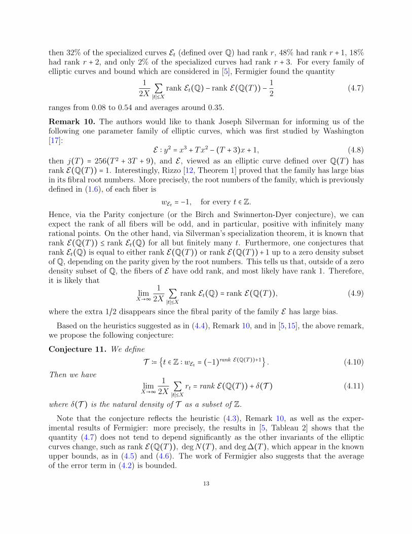
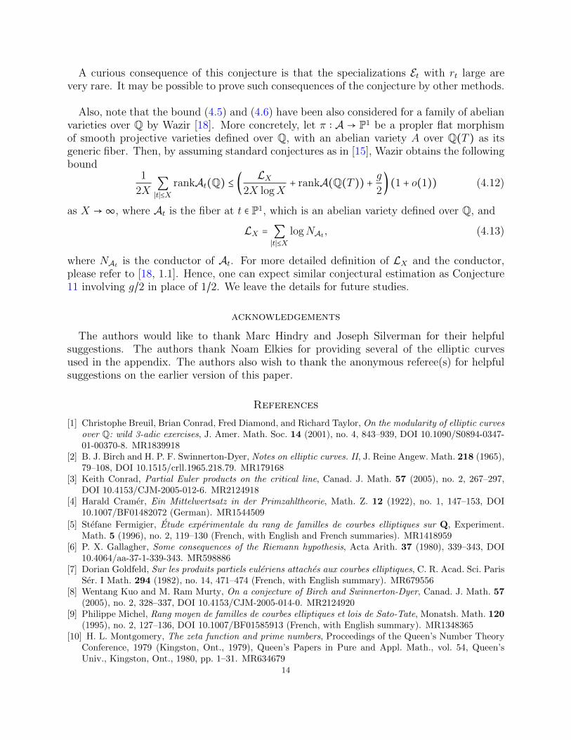
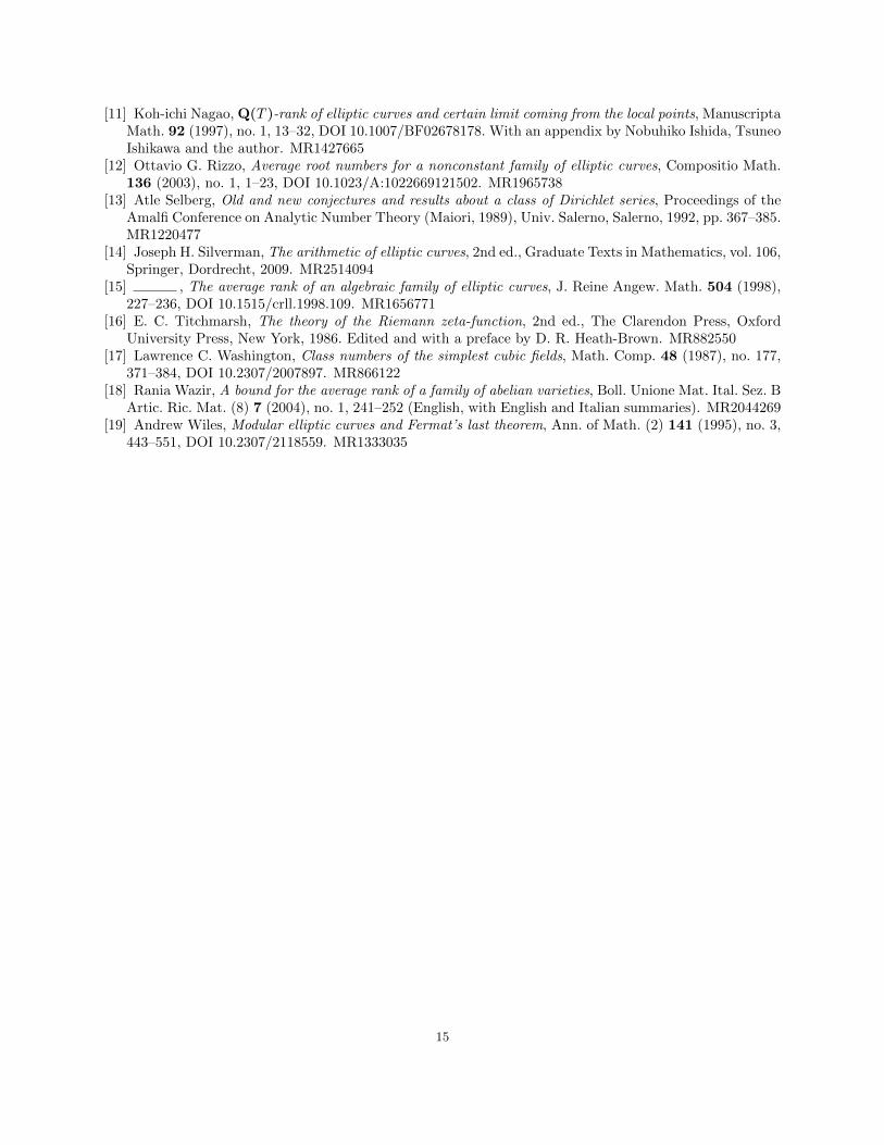
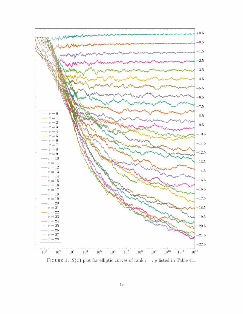
Let ap(E) denote the Frobenius trace of an elliptic curve E/Q at a prime p. Figures 1, 2,3 plot the sums

S(x) ∶= 1

logx∑

p≤x, p∤∆E

ap(E) log p

p

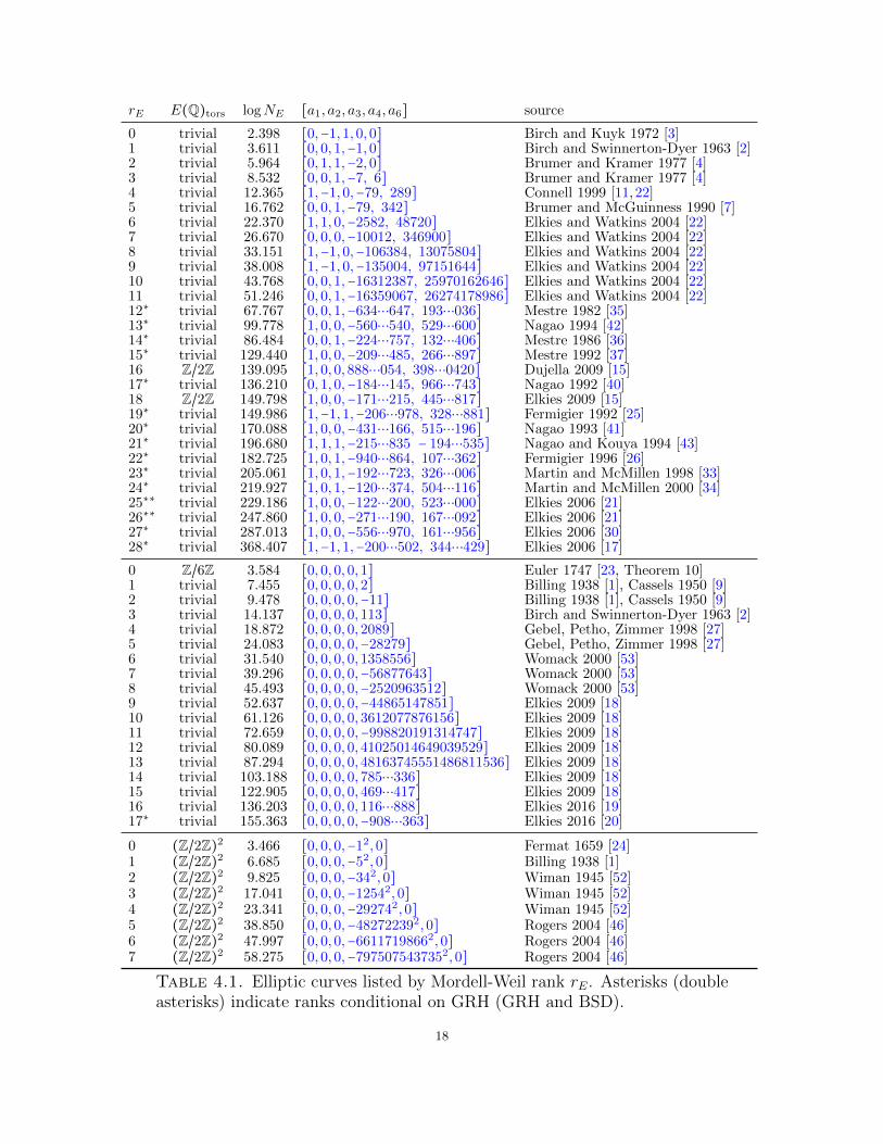
for elliptic curves E of discriminant ∆E and various ranks; See Table 4.1 for a list of thecurves and their sources. These sums are conjectured to converge to r−1/2 as x→∞, wherer is the analytic rank of LE(s). The ranks rE listed in Table 4.1 are lower bounds on theMordell-Weil rank that are also upper bounds on the analytic rank under the GeneralizedRiemann Hypothesis (GRH), and equal to both the Mordell-Weil rank and the analytic rankunder the Birch and Swinnerton–Dyer conjecture (BSD). Ranks listed with no asterisk areequal to the Mordell-Weil rank; for those marked with a single (resp. double) asterisk thisequality is conditional on GRH (resp. GRH and BSD). Lower bounds on the Mordell-Weilrank were confirmed by verifying the existence of rE independent points using the Neron-Tateheight pairing, while GRH-based upper bounds on the analytic rank were confirmed usingBober’s method [6]. GRH-based upper bounds on the Mordell-Weil rank were confirmedusing magma [5] for rE ≤ 19; for rE ≥ 20 we rely on the results of [30]. Exact values ofMordell-Weil ranks were confirmed using Cremona’s mwrank [14] package for rE ≤ 11; forranks rE ≥ 12 with no asterisk we rely on computations reported in the listed sources. Thecurves of rank rE ≤ 11 have conductors NE that are close to the smallest possible [22]. This isnot likely to be true for the curves for rank rE ≥ 12, but we chose curves of smaller conductorwhen several were available. In many cases the curves we list are not the first known curveof that rank; see [16] for a history of rank records.

The sums S(x) plotted for x ≤ B = 1012 in Figure 1 were computed using the smalljac

software library [29] with some further optimizations described in [48, 49]. The expectedtime complexity of this approach is O(B5/4 logB log logB). This is asymptotically worsethan both the O(B(logB)4+o(1)) expected time complexity (under GRH) of using the Schoof-Elkies-Atkin algorithm [50] and the O(B(logB)3) time complexity of an average polynomial-time approach [28], but it is practically much faster for B = 1012; it took approximately 100core-days per curve to compute the S(x) plots shown in Figure 1.

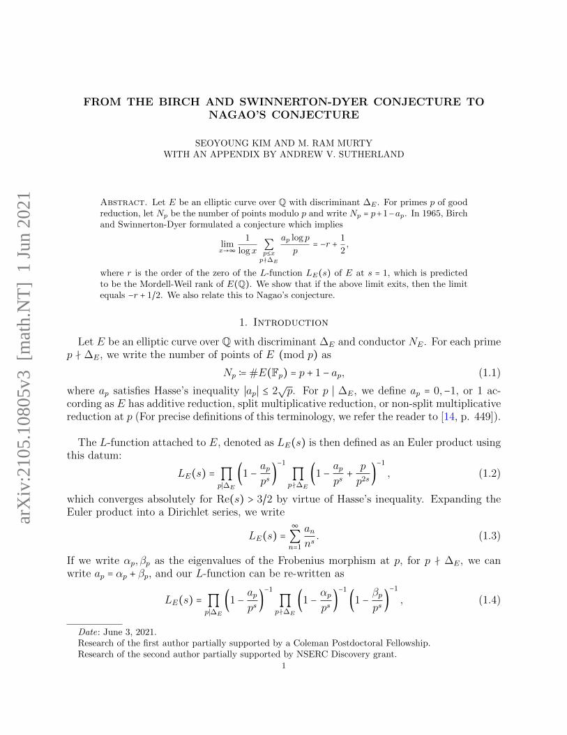
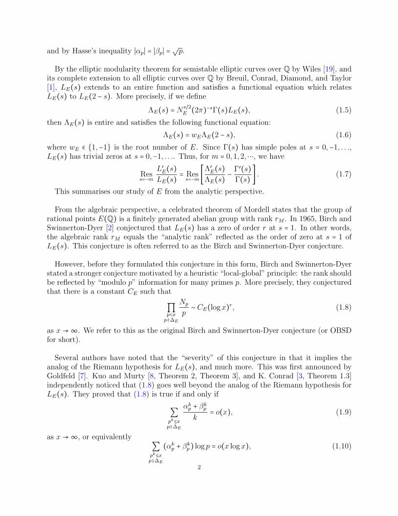
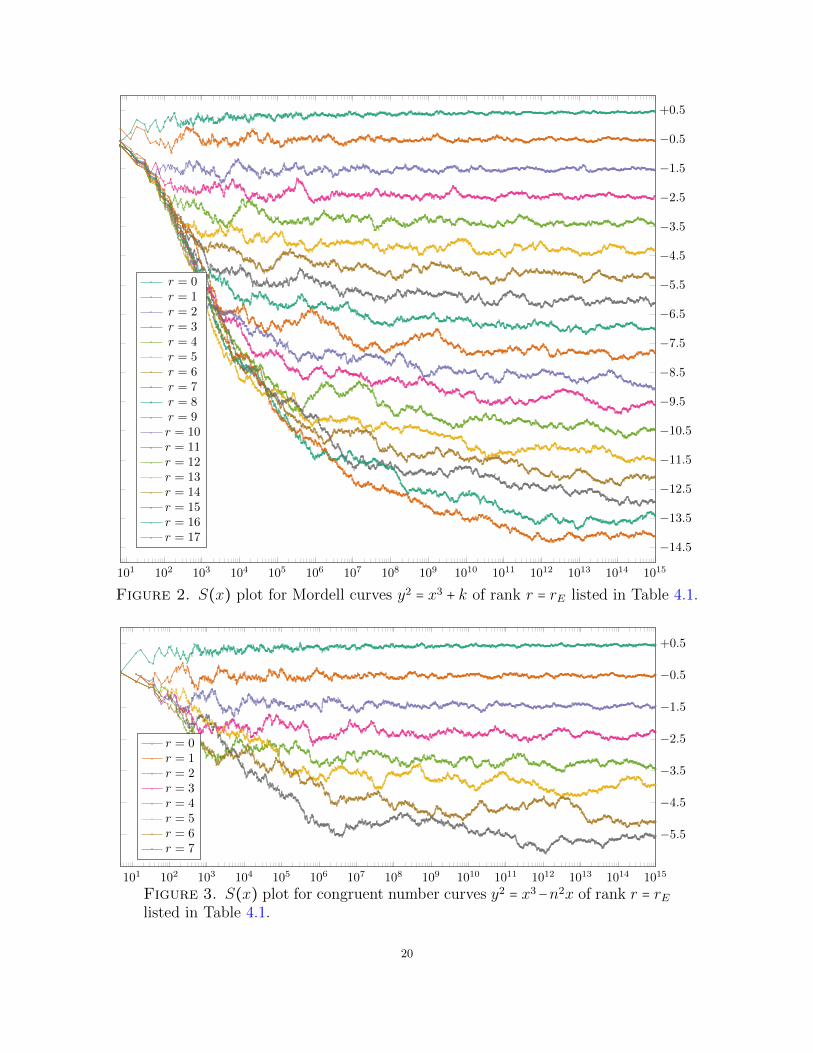
Figures 2 and 3 show similar plots for Mordell curves [38] y2 = x3 + k of ranks rE =0,1,2, . . . ,17 and congruent number curves [39] y2 = x3 −n2x of ranks rE = 0,1,2, . . . ,7. Thecorresponding curves listed in Table 4.1 were chosen to minimize ∣k∣ and n among those of agiven rank which have appeared in the literature (we chose the sign of k yielding a smallerconductor). These are not necessarily the first curves of these forms found to achieve theseranks; see [32,44,53] for some earlier examples.

The Mordell curves and congruent number curves have j-invariants 0,1728 (respectively),and thus admit (potential) complex multiplication by the ring of integersO ofK = Q(ζ3),Q(i).To efficiently compute ap(E) = tr(ψE(p)) we compute the trace of the Hecke character ψEcorresponding to E evaluated at a prime p of K above p; this trace is necessarily zero when

1Department of Mathematics, Massachusetts Institute of Technology, 77 Massachusetts Ave., Cambridge,MA 02139, USA; email: drew@math.mit.edu, URL: https://math.mit.edu/~drew. Supported by SimonsFoundation grant 550033.

16

p is inert. For each prime p ≤ B of good reduction for E that splits in O we use Cornacchia’salgorithm to compute all integer solutions (t, v) to the norm equation 4p = t2 − v2disc(O).We then apply the algorithm of Rubin and Silverberg [47] to determine the correct choice oft = ap. The algorithm in [47] determines the correct twist of an ordinary elliptic curve over Fpwith a given j-invariant, endomorphism ring and Frobenius trace, but it can also be usedto determine the Frobenius trace of an ordinary elliptic curve over Fp whose endomorphismring is known. This yields an algorithm to compute ap(E) in O((log p)2 log log p) expectedtime, meaning we can compute S(x) for x ≤ B in O(B logB log logB) expected time. Thismakes it feasible to plot S(x) for x ≤ B = 1015 in Figures 2 and 3 in roughly the same timerequired for B = 1012 in Figure 1, about 100 core-days per curve.

We end with a note of caution regarding the interpretation of these plots as evidencesupporting the conjectured convergence of S(x). The methods used to find the higher rankcurves shown in these plots typically use S(x) or a closely related sum as a heuristic methodto identify elliptic curves of potentially high rank; see [8, 36, 42]. Most of the curves of rankrE ≥ 12 listed in Table 4.1 were discovered precisely because a partial sum related to S(x)suggested they should have large ranks. This is less of a concern for the lower rank curveswhere searches have been more exhaustive in an effort to minimize NE, ∣k∣, or n.

17

rE E(Q)tors logNE [a1, a2, a3, a4, a6] source

0 trivial 2.398 [0,−1,1,0,0] Birch and Kuyk 1972 [3]1 trivial 3.611 [0,0,1,−1,0] Birch and Swinnerton-Dyer 1963 [2]2 trivial 5.964 [0,1,1,−2,0] Brumer and Kramer 1977 [4]3 trivial 8.532 [0,0,1,−7, 6] Brumer and Kramer 1977 [4]4 trivial 12.365 [1,−1,0,−79, 289] Connell 1999 [11,22]5 trivial 16.762 [0,0,1,−79, 342] Brumer and McGuinness 1990 [7]6 trivial 22.370 [1,1,0,−2582, 48720] Elkies and Watkins 2004 [22]7 trivial 26.670 [0,0,0,−10012, 346900] Elkies and Watkins 2004 [22]8 trivial 33.151 [1,−1,0,−106384, 13075804] Elkies and Watkins 2004 [22]9 trivial 38.008 [1,−1,0,−135004, 97151644] Elkies and Watkins 2004 [22]10 trivial 43.768 [0,0,1,−16312387, 25970162646] Elkies and Watkins 2004 [22]11 trivial 51.246 [0,0,1,−16359067, 26274178986] Elkies and Watkins 2004 [22]12∗ trivial 67.767 [0,0,1,−634⋯647, 193⋯036] Mestre 1982 [35]13∗ trivial 99.778 [1,0,0,−560⋯540, 529⋯600] Nagao 1994 [42]14∗ trivial 86.484 [0,0,1,−224⋯757, 132⋯406] Mestre 1986 [36]15∗ trivial 129.440 [1,0,0,−209⋯485, 266⋯897] Mestre 1992 [37]16 Z/2Z 139.095 [1,0,0,888⋯054, 398⋯0420] Dujella 2009 [15]17∗ trivial 136.210 [0,1,0,−184⋯145, 966⋯743] Nagao 1992 [40]18 Z/2Z 149.798 [1,0,0,−171⋯215, 445⋯817] Elkies 2009 [15]19∗ trivial 149.986 [1,−1,1,−206⋯978, 328⋯881] Fermigier 1992 [25]20∗ trivial 170.088 [1,0,0,−431⋯166, 515⋯196] Nagao 1993 [41]21∗ trivial 196.680 [1,1,1,−215⋯835 − 194⋯535] Nagao and Kouya 1994 [43]22∗ trivial 182.725 [1,0,1,−940⋯864, 107⋯362] Fermigier 1996 [26]23∗ trivial 205.061 [1,0,1,−192⋯723, 326⋯006] Martin and McMillen 1998 [33]24∗ trivial 219.927 [1,0,1,−120⋯374, 504⋯116] Martin and McMillen 2000 [34]25∗∗ trivial 229.186 [1,0,0,−122⋯200, 523⋯000] Elkies 2006 [21]26∗∗ trivial 247.860 [1,0,0,−271⋯190, 167⋯092] Elkies 2006 [21]27∗ trivial 287.013 [1,0,0,−556⋯970, 161⋯956] Elkies 2006 [30]28∗ trivial 368.407 [1,−1,1,−200⋯502, 344⋯429] Elkies 2006 [17]

0 Z/6Z 3.584 [0,0,0,0,1] Euler 1747 [23, Theorem 10]1 trivial 7.455 [0,0,0,0,2] Billing 1938 [1], Cassels 1950 [9]2 trivial 9.478 [0,0,0,0,−11] Billing 1938 [1], Cassels 1950 [9]3 trivial 14.137 [0,0,0,0,113] Birch and Swinnerton-Dyer 1963 [2]4 trivial 18.872 [0,0,0,0,2089] Gebel, Petho, Zimmer 1998 [27]5 trivial 24.083 [0,0,0,0,−28279] Gebel, Petho, Zimmer 1998 [27]6 trivial 31.540 [0,0,0,0,1358556] Womack 2000 [53]7 trivial 39.296 [0,0,0,0,−56877643] Womack 2000 [53]8 trivial 45.493 [0,0,0,0,−2520963512] Womack 2000 [53]9 trivial 52.637 [0,0,0,0,−44865147851] Elkies 2009 [18]10 trivial 61.126 [0,0,0,0,3612077876156] Elkies 2009 [18]11 trivial 72.659 [0,0,0,0,−998820191314747] Elkies 2009 [18]12 trivial 80.089 [0,0,0,0,41025014649039529] Elkies 2009 [18]13 trivial 87.294 [0,0,0,0,48163745551486811536] Elkies 2009 [18]14 trivial 103.188 [0,0,0,0,785⋯336] Elkies 2009 [18]15 trivial 122.905 [0,0,0,0,469⋯417] Elkies 2009 [18]16 trivial 136.203 [0,0,0,0,116⋯888] Elkies 2016 [19]17∗ trivial 155.363 [0,0,0,0,−908⋯363] Elkies 2016 [20]

0 (Z/2Z)2 3.466 [0,0,0,−12,0] Fermat 1659 [24]1 (Z/2Z)2 6.685 [0,0,0,−52,0] Billing 1938 [1]2 (Z/2Z)2 9.825 [0,0,0,−342,0] Wiman 1945 [52]3 (Z/2Z)2 17.041 [0,0,0,−12542,0] Wiman 1945 [52]4 (Z/2Z)2 23.341 [0,0,0,−292742,0] Wiman 1945 [52]5 (Z/2Z)2 38.850 [0,0,0,−482722392,0] Rogers 2004 [46]6 (Z/2Z)2 47.997 [0,0,0,−66117198662,0] Rogers 2004 [46]7 (Z/2Z)2 58.275 [0,0,0,−7975075437352,0] Rogers 2004 [46]

Table 4.1. Elliptic curves listed by Mordell-Weil rank rE. Asterisks (doubleasterisks) indicate ranks conditional on GRH (GRH and BSD).

18

101 102 103 104 105 106 107 108 109 1010 1011 1012

−22.5

−21.5

−20.5

−19.5

−18.5

−17.5

−16.5

−15.5

−14.5

−13.5

−12.5

−11.5

−10.5

−9.5

−8.5

−7.5

−6.5

−5.5

−4.5

−3.5

−2.5

−1.5

−0.5

+0.5

r = 0r = 1r = 2r = 3r = 4r = 5r = 6r = 7r = 8r = 9r = 10r = 11r = 12r = 13r = 14r = 15r = 16r = 17r = 18r = 19r = 20r = 21r = 22r = 23r = 24r = 25r = 26r = 27r = 28

Figure 1. S(x) plot for elliptic curves of rank r = rE listed in Table 4.1.

19

101 102 103 104 105 106 107 108 109 1010 1011 1012 1013 1014 1015

−14.5

−13.5

−12.5

−11.5

−10.5

−9.5

−8.5

−7.5

−6.5

−5.5

−4.5

−3.5

−2.5

−1.5

−0.5

+0.5

r = 0r = 1r = 2r = 3r = 4r = 5r = 6r = 7r = 8r = 9r = 10r = 11r = 12r = 13r = 14r = 15r = 16r = 17

Figure 2. S(x) plot for Mordell curves y2 = x3 + k of rank r = rE listed in Table 4.1.

101 102 103 104 105 106 107 108 109 1010 1011 1012 1013 1014 1015

−5.5

−4.5

−3.5

−2.5

−1.5

−0.5

+0.5

r = 0r = 1r = 2r = 3r = 4r = 5r = 6r = 7

Figure 3. S(x) plot for congruent number curves y2 = x3−n2x of rank r = rElisted in Table 4.1.

20

References

[1] Gunnar Billing, Beitrage zur arithmetischen Theorie ebener kubischer Kurven, Nova Acta Reg. Soc.Scient. Upsaliensis. Ser. IV vol XI (1938), 1–165.

[2] Bryan J. Birch and H.P.F. Swinnerton-Dyer, Notes on elliptic curves. I., J. Reine Angew. Math. 212(1963), 7–25.

[3] Bryan J. Birch and Willem Kuyk, Table 1, in Modular Functions of One Variable IV, Proceedings of theInternational Summer School, University of Antwerp, RUCA, July 17–August 3, 1972, Lecture Notes inMath. 476, Springer, 1975.

[4] Armand Brumer and Kenneth Kramer, The rank of elliptic curves, Duke Math. J. 44 (1977), 715–743.[5] W. Bosma, J.J. Cannon, C. Fieker, and A. Steel (Eds.), Handbook of Magma functions, v2.26-1, 2021.[6] Jonathan Bober, Conditionally bounding analytic ranks of elliptic curves, in Proceedings of the Tenth

Algorithmic Number Theory Symposium (ANTS X), Open Book Series 1, 2013, 135–144.[7] Armand Brumer and Oisin McGuinness, The behaviour of the Mordell-Weil group of elliptic curves,

Bulletin of the AMS 23 (Oct 1990), 375–382.[8] Garikai Campbell, Finding elliptic curves and families of elliptic curves over Q of large rank , Ph.D.

Thesis, Rutgers, 1999.[9] J.W.S. Cassels, The rational solutions of the diophantine equation y2 = x3 −D, Acta Math. 82 (1950),

242–273.[10] Ian Connell, Elliptic curve handbook , McGill University, 1999.[11] Ian Connell, Arithmetic of plane elliptic curves (APECS), Maple software package described in [10, pp.

160–166], 1999.[12] John E. Cremona, Algorithms for modular elliptic curves, 2nd ed., Cambridge Univ. Press, Cambridge,

1997.[13] John E. Cremona, Minimal conductor of an elliptic curve over Q of rank 4, NMBRTHRY listserv post,

available at https://listserv.nodak.edu/cgi-bin/wa.exe?A2=NMBRTHRY;6f6148dc.1204.[14] John E. Cremona, eclib, GitHub repository available at https://github.com/JohnCremona/eclib,

accessed May 1, 2021.[15] Andrej Dujella, Elliptic curves of high rank with prescribed torsion (old version), including curves of

rank 16 and 18 due to Dujella and Elkies (resp.), available at https://web.math.pmf.unizg.hr/~duje/tors/z2old1415161718.html.

[16] Andrej Dujella, History of elliptic curves rank records, available at https://web.math.pmf.unizg.hr/

~duje/tors/rankhist.html.[17] Noam D. Elkies, Z28 in E(Q), etc., NMBRTHRY listerv post, available at https://listserv.nodak.

edu/cgi-bin/wa.exe?A2=NMBRTHRY;99f4e7cd.0605, May 3, 2006.[18] Noam D. Elkies, j = 0, rank 15; also 3-rank 6 and 7 in real and imaginary quadratic fields, NM-

BRTHRY listserv post, available at https://listserv.nodak.edu/cgi-bin/wa.exe?A2=NMBRTHRY;

6a3fad67.0912, December 30, 2009.[19] Noam D. Elkies, j = 0, rank 16; also 3-rank 7 and 8 in real and imaginary quadratic fields, NM-

BRTHRY listserv post, available at https://listserv.nodak.edu/cgi-bin/wa.exe?A2=NMBRTHRY;

fc0d1ed0.1602, February 6, 2016.[20] Noam D. Elkies, How many points can a curve have? , talk given at Arizona State University (Tempe),

slides available at http://math.harvard.edu/~elkies/many_pts_asu.pdf, February 18, 2016.[21] Noam D. Elkies, Missing elliptic curve ranks, personal email, received January 7, 2021.[22] Noam D. Elkies and Mark Watkins, Elliptic curves of large rank and small conductor , in Algorithmic

Number Theory Symposium (ANTX VI), pp. 42–56, Lecture Notes in Computer Science 3076, Springer,2004.

[23] Leonhard Euler, Theorematum quorundam arithmeticorum demonstrationes, Commentarii academiaescientiarum Petropolitanae 10 (1747), 125–146.

[24] Pierre Fermat, Letter to Pierre de Carcavi, August 1659, pages 431–436 in Oeuvres de Fermat 2, P.Tannery and C. Henry (Eds.), Guathier-Villars, Paris, 1894.

[25] Stefane Fermigier, Un exemple de courbe elliptique definie sur Q de rang ≥ 19, C. R. Acad. Sci. ParisSer. I Math. 315 (1992), 719–722;

21

[26] Stefane Fermigier, An elliptic curve of rank ≥ 22 over Q, NMBRTHRY listserv post, available at https://listserv.nodak.edu/cgi-bin/wa.exe?A2=NMBRTHRY;5a3fefaa.9607, July 7, 1996.

[27] Josef Gebel, Attila Petho, Horst G. Zimmer, On Mordell’s equation, Compositio Math. 110 (1998),335–367.

[28] David Harvey and Andrew V. Sutherland, Computing Hasse–Witt matrices of hyperelliptic curves inaverage polynomial-time, in Frobenius distributions: Lang–Trotter and Sato–Tate conjectures, Contemp.Math. 663 (2016), 103–126.

[29] Kiran S. Kedlaya and Andrew V. Sutherland, Computing L-series of hyperelliptic curves, in AlgorithmicNumber Theory 8th International Symposium (ANTS VIII), Lecture Notes in Computer Science 5011,Springer, 2008, 312–326.

[30] Zev Klagsbrun, Travis Sherman, and James Weigandt, The Elkies curve has rank 28 subject only toGRH , Math. Comp. 88 (2019), 837–846.

[31] The LMFDB Collaboration, The L-functions and Modular Forms Database, http://www.lmfdb.org,2021.

[32] Pascal Llorente and Jordi Quer, On the 3-Sylow subgroup of the class group of quadratic fields, Math.Comp. 50 (1988), 321–333.

[33] Roland Martin and William McMillen, An elliptic curve/Q of rank 23, NMBRTHRY listserv post,available at https://listserv.nodak.edu/cgi-bin/wa.exe?A2=NMBRTHRY;d3867479.9803, March 16,1998.

[34] Roland Martin and William McMillen, An elliptic curve/Q of rank 24, NMBRTHRY listserv post, avail-able at https://listserv.nodak.edu/cgi-bin/wa.exe?A2=NMBRTHRY;b8b5e7f2.0005, May 2, 2000.

[35] Jean-Francois Mestre, Construction d’une courbe elliptique de rang ≥ 12, C.R. Acad. Sci. Pari. Ser. IMath. 295 (1982), 643–644.

[36] Jean-Francois Mestre, Formules explicites et minorations de conducteurs de varietes algebriques, Com-positio Math. 58 (1986), 209–232.

[37] Jean-Francois Mestre, Un exemple de courbe elliptique sur Q de rang ≥ 15, C.R. Acad. Sci. Pari. Ser. IMath. 314 (1992), 454–455.

[38] Louis J. Mordell, The diophantine equation y2 − k = x3, Proc. London Math. Soc. 13 (1914), 60–80.[39] Louis J. Mordell, On the rational solutions of the indeterminate equations of the third and fourth degree,

Proc. Cambr. Philos. Soc. 21 (1922), 179–192.[40] Koh-ichi Nagao, Examples of elliptic curves over Q with rank ≥ 17, Proc. Japan Acad. Ser. A Math.

Sci. 68 (1992), 287–289.[41] Koh-ichi Nagao, An example of elliptic curve over Q with rank ≥ 20, Proc. Japan Acad. ser. A Math.

Sci. 69 (1993), 291–293.[42] Koh–ichi Nagao, An example of elliptic curve over Q(T ) with rank ≥ 13, Proc. Japan Acad. Ser. A

Math. Sci. 70 (1994), 152–153.[43] Koh-ichi Nagao et Tomonori Kouya, An example of elliptic curve over Q with rank > 21, Proc. Japan

Acad. Ser. A, 70 (1994), p. 104–105;[44] Jordi Quer, Corps quadratiques de 3-rang 6 et courbes elliptiques de rang 12, C. R. Acad. Sci. Paris Ser.

I Math. 305 (1987), 215–218.[45] Nicholas F. Rogers, Rank computations for the congruent number elliptic curves, Experiment Math. 9

(2000), 591–594.[46] Nicholas F. Rogers, Elliptic curves x3 + y3 = k with high rank , Ph.D. Thesis, Harvard University, 2004.[47] Karl Rubin and Alice Silverberg, Choosing the correct elliptic curve in the CM method , Math. Comp.

79 (2010), 545–561.[48] Andrew V. Sutherland, Order computations in generic groups, Ph.D. Thesis, Massachusetts Institute

of Technology, 2007.[49] Andrew V. Sutherland, Structure computation and discrete logarithms in finite abelian p-groups, Math.

Comp. 80 (2011), 477–500.[50] Igor E. Shparlinski and Andrew V. Sutherland, On the distribution of Atkin and Elkies primes for

reductions of elliptic curves on average, LMS J. Comput. Math. 18 (2015), 308–322.[51] Mark Watkins, Stephen Donnelly, Noam D. Elkies, Tom Fisher, Andrew Granville, and Nicholas Roger,

Ranks of quadratic twists of elliptic curves, Publ. Math. Besancon Algebre Theorie Nr. 2014/2, 63–98.

22

[52] A. Wiman, Uber rationale Punkte auf Kurven y2 = x(x2 − c2), Acta Math. 77 (1945), 281–320.[53] Tom Womack, Minimal-known positive and negative k for Mordell curves of given rank , web page snap-

shot available at https://web.archive.org/web/20000925204914/http://tom.womack.net/maths/

mordellc.htm, September 25, 2000.

Email address: sk206@queensu.ca

Department of Mathematics and Statistics, Queen’s University, Kingston, ON, CanadaK7L 3N6

Email address: murty@queensu.ca

Department of Mathematics and Statistics, Queen’s University, Kingston, ON, CanadaK7L 3N6

23