From Tree Tensor Network to Multiscale Entanglement Renormalization Ansatz

Xiangjian Qian1 and Mingpu Qin1, ∗

1Key Laboratory of Artificial Structures and Quantum Control (Ministry of Education),School of Physics and Astronomy, Shanghai Jiao Tong University, Shanghai 200240, China

Tensor Network States (TNS) offer an efficient representation for the ground state of quantummany body systems and play an important role in the simulations of them. Numerous TNS areproposed in the past few decades. However, due to the high cost of TNS for two-dimensional systems,a balance between the encoded entanglement and computational complexity of TNS is yet to bereached. In this work we introduce a new Tree Tensor Network (TTN) based TNS dubbed as Fully-Augmented Tree Tensor Network (FATTN) by releasing the constraint in Augmented Tree TensorNetwork (ATTN). When disentanglers are augmented in the physical layer of TTN, FATTN canprovide more entanglement than TTN and ATTN. At the same time, FATTN maintains the scalingof computational cost with bond dimension in TTN and ATTN. Benchmark results on the groundstate energy for the transverse Ising model are provided to demonstrate the improvement of accuracyof FATTN over TTN and ATTN. Moreover, FATTN is quite flexible which can be constructed as aninterpolation between Tree Tensor Network and Multiscale Entanglement Renormalization Ansatz(MERA) to reach a balance between the encoded entanglement and the computational cost.

I. INTRODUCTION

Understanding exotic phases and exotic phase transi-tions in strongly correlated quantum many body systemsis one of the most challenging topics in condensed matterphysics [1–3]. Due to the lack of analytic solutions, moststudies of these systems depend on many-body numer-ical approaches [4]. For quantum many body systems,the exponential increase of the dimension of the Hilbertspace prevents us from studying system with large sizes.Quantum Monte Carlo is an efficient method for quantummany body systems, but it usually suffers from the in-famous minus sign problem for Fermionic systems [5, 6].For a local Hamiltonian, the ground state and low en-ergy excited states satisfy the well-known entanglement-entropic area law [7–10], asserting that if we divide thestudied system into two parts, the entanglement entropyis proportional to the measure of the partition’s bound-ary rather than its volume. Hence, if we are only in-terested in the low-lying states, we only need to con-sider states which satisfy the entanglement-entropic arealaw in the Hilbert space. Tensor Network States (TNS)[11–13] can efficiently encode the entanglement-entropicarea law by design, which can faithfully represent theground state of quantum many body systems. In recentyears, significant advances in TNS have been made andthey are becoming one of the most popular approachesin studying strongly correlated quantum many body sys-tems [14, 15]. During the last three decades, after real-izing the underlying wave-functions in Density MatrixRenormalization Group (DMRG) [16–21] are actuallyMatrix Product States (MPS) [22, 23], several types ofTNS for higher dimensional systems are proposed, in-cluding Tree Tensor Network (TTN) [24–27], ProjectedEntanglement Pair States (PEPS) [28–30] and their gen-

∗qinmingpu@sjtu.edu.cn

eralization [31], and Multiscale Entanglement Renormal-ization Ansatz (MERA) [32–35].

For (quasi) one dimensional systems, DMRG or MPSbased approaches [18, 19] are now the workhorse as itcan capture the one dimensional entanglement-entropicarea law (with a logarithmic correction for critical sys-tems) with a relatively low computational complexity.However, to study two-dimensional systems with DMRG,the bond-dimension needs to be increased exponentiallywith the width of the system to be able to capture theentanglement-entropic area law, which makes the studyof wide system difficult with DMRG [36]. PEPS is astraightforward generalization of MPS to two dimension.It can capture the area-law of entanglement entropy fortwo-dimensional systems by design. However, it suffersfrom a high computational complexity which is usuallyhigher than O(D10) [37, 38], with D the bond-dimensionof PEPS. Moreover, the overlap of PEPSs can’t be cal-culated exactly [39], even though there exist many ap-proaches to calculate it approximately [12, 40, 41]. Onthe contrary, MERA which is constructed by unitary ten-sors [42], can be contracted exactly but suffers from amuch higher computational complexity for two dimen-sional systems O(D16) [33]. TTN has a similar struc-ture to MERA. It has a lower computational complexityfor two dimensional systems (O(D4)), but encounters thesame problems as the DMRG in 2D because TTN doesn’tencode the two-dimensional entanglement-entropic arealaw by design. So it is desirable to develop new ten-sor networks with affordable computational complexitywhich can also encode high entanglement.

Recently, a new tensor network structure based onTTN: Augmented Tree Tensor Network (ATTN) was pro-posed in [43]. By placing disentanglers at the physicallayer of a TTN, it was claimed that ATTN can capturethe entanglement-entropic area-law and at the same timekeep a computational complexity of O(D4d2), with d thedimension of the physical degree of freedom.

We propose a new structure which can provide larger

arX

iv:2

110.

0879

4v1

[qu

ant-

ph]

17

Oct

202

1

2

𝛼 𝛽

𝛾

(a) (b) (c)

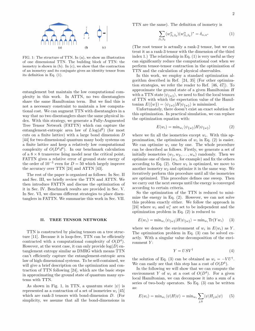
FIG. 1: The structure of TTN. In (a), we show an illustrationof one dimensional TTN. The building block of TTN: theisometry is shown in (b). In (c), we show that the contractionof an isometry and its conjugate gives an identity tensor fromits definition in Eq. (1).

entanglement but maintain the low computational com-plexity in this work. In ATTN, no two disentanglersshare the same Hamiltonian term. But we find this isnot a necessary constraint to maintain a low computa-tional cost. We can augment TTN with disentanglers in away that no two disentanglers share the same physical in-dex. With this strategy, we generate a Fully-AugmentedTree Tensor Network (FATTN) which can capture theentanglement-entropic area law of L log(d2) (for mostcuts on a finite lattice) with a large bond dimension D[44] for two-dimensional quantum many body systems ona finite lattice and keep a relatively low computationalcomplexity of O(D4d4). In our benchmark calculationof a 8× 8 transverse Ising model near the critical point,FATTN gives a relative error of ground state energy ofthe order of 10−5 even for D = 50 which largely improvethe accuracy over TTN [24] and ATTN [43].

The rest of the paper is organized as follows: In Sec. IIand Sec. III, we briefly review the TTN and ATTN. Wethen introduce FATTN and discuss the optimization ofit in Sec. IV. Benchmark results are provided in Sec. V.In Sec. VI, we discuss different strategies to place disen-tanglers in FATTN. We summarize this work in Sec. VII.

II. TREE TENSOR NETWORK

TTN is constructed by placing tensors on a tree struc-ture [11]. Because it is loop-free, TTN can be efficientlycontracted with a computational complexity of O(D4).However, at the worst case, it can only provide log(D) en-tanglement entropy similar as DMRG which means TTNcan’t efficiently capture the entanglement-entropic arealaw of high dimensional systems. To be self-contained, wewill give a brief description on the optimization and con-traction of TTN following [24], which are the basic stepsin approximating the ground state of quantum many sys-tems with TTN.

As shown in Fig. 1, in TTN, a quantum state |ψ〉 isrepresented as a contraction of a set of isometries wi [45]which are rank-3 tensors with bond-dimension D. (Forsimplicity, we assume that all the bond-dimensions in

TTN are the same). The definition of isometry is∑β1β2

(wαβ1β2)(wαβ1β2

)∗ = δα,α∗ (1)

(The root tensor is actually a rank-2 tensor, but we cantreat it as a rank-3 tensor with the dimension of the thirdindex 1.) The relationship in Eq. (1) is very useful as theycan significantly reduce the computational cost when weperform tensor-tensor contraction in the optimization ofTTN and the calculation of physical observables.

In this work, we employ a standard optimization al-gorithm described in Ref. [24, 35] (For other optimiza-tion strategies, we refer the reader to Ref. [46, 47]). Toapproximate the ground state of a given Hamiltonian Hwith a TTN state |ψ{w}〉, we need to find the local tensorsof TTN with which the expectation value of the Hamil-tonian E({w}) = 〈ψ{w}|H|ψ{w}〉 is minimized.

Unfortunately, there doesn’t exist an exact solution forthis optimization. In practical simulation, we can replacethe optimization equation with:

E(wi) = minwi〈ψ{w}|H|ψ{w}〉 (2)

where we fix all the isometries except wi. With this ap-proximation, the optimization of wi in Eq. (2) is easier.We can optimize wi one by one. The whole procedurecan be described as follows. Firstly, we generate a set ofinitially isometries (w1, w2, . . . , wn) randomly. Then weoptimize one of them (w1, for example) and fix the othersaccording to Eq. (2). Once w1 is optimized, we move toanother isometry w2 and optimize it in the same way. Weiteratively perform this procedure until all the isometriesare optimized. This procedure defines one sweep. Thenwe carry out the next sweeps until the energy is convergedaccording to certain criteria.

So the optimization of the TTN is reduced to mini-mize the energy in Eq. (2). However, we can not solvethis problem exactly either. We follow the approach in[24] where wi and w∗i are set to be independent and theoptimization problem in Eq. (2) is reduced to

E(wi) = minwi〈ψ{w}|H|ψ{w}〉 = minwi

Tr(Y wi) (3)

where we denote the environment of wi in E(wi) as Y .The optimization problem in Eq. (3) can be solved ex-actly. With a singular value decomposition of the envi-ronment Y :

Y = USV † (4)

the solution of Eq. (3) can be obtained as wi = −V U†.We can easily see that this step has a cost of O(D4).

In the following we will show that we can compute theenvironment Y of wi at a cost of O(D4). For a givenlocal Hamiltonian, we can decompose it into a sum of aseries of two-body operators. So Eq. (3) can be writtenas:

E(wi) = minwi〈ψ|H|ψ〉 = minwi

∑j,k

〈ψ|Hj,k|ψ〉 (5)

3

(a) (b)

(c) (d) (e)

FIG. 2: The calculation of the environment for an isome-try. We can see that every step has a computational cost ofO(D4). And the contractions which are not connected withthe Hamiltonian term (denoted as the yellow circles) are justidentities because of Eq. (1).

E

𝑆𝑉𝐷

𝑈 𝑆 𝑉

𝑉

𝑈

isometry

(a) (b)

(c) (d)

FIG. 3: The optimization of the isometry. After the environ-ment tensor Y is obtained, a SVD decomposition of it is per-formed Y = USV †. The optimized wi is set as wi = −V U†.This step also takes a computational cost of O(D4).

where j, k denote the position of the two-body operator.

Therefore, without loss of generality, we only need todeal with two-site operator (one site term is easy to han-dle as discussed below). We can further decompose thetwo-site operator into a sum of direct product of two one-site operators whose number is d2 in the worst case withd the dimension of the physical degree of freedom at the

FIG. 4: The strategy to place disentanglers in ATTN. In orderto maintain the same O(D4) scaling of computational cost asin TTN, no couple of disentanglers are directly connected by aHamiltonian term. As will be discussed late in the main text,this is not a necessary constraint to keep the O(D4) cost.

physical layer of TTN. Once we compute the contribu-tions from all the terms in the Hamiltonian, we simplyadd those contributions to get the environment Y . Asshown in Fig. 2, the calculation of the environment Y ofwi for a two-site operator has a cost of O(D4). We cantake advantage of Eq. (1) to simplify the calculation asthe contraction of two conjugated isometrics results inan identity tensor if there is no operator acting on them.As the singular value decomposition of Y has a cost ofO(D4), the overall cost to optimize a TTN is O(D4). It iseasily to show that the calculation of physical observablesalso have a cost ofO(D4). So it is efficient to approximatethe ground state of a local quantum Hamiltonian with aTTN. But as mentioned earlier, TTN can’t capture theentanglement-entropic area law for systems in spatial di-mension larger than two which hamper its application insimulating two-dimensional many-body systems.

III. AUGMENTED TREE TENSOR NETWORK

ATTN [43] was proposed to provide more entangle-ment entropy than TTN. By placing disentanglers whichare unitary tensors satisfying the following condition:∑

β1β2

(uα1α2

β1β2)(uα1α2

β1β2)∗ = δα1α2,(α1α2)∗ (6)

at the physical layer of TTN, the entanglement entropyencode in ATTN scales as L log(d) [43]. In ATTN, nocouple of disentanglers are directly connected by an in-teraction term in the Hamiltonian to keep a low compu-tational cost. ATTN has a computational complexity ofO(D4d2) which has the same scaling of D as the TTN.However, a large improvement in numerical precision ofATTN over TTN was shown in [43].

In Fig. 4 we show the strategies of placing the disentan-glers in ATTN for a 8×8 lattice. We can see that a rela-

4

tively small number of disentanglers are placed to encodethe entanglement-entropic area law under the conditionthat no couple of disentanglers share the same Hamilto-nian term.

IV. FULLY-AUGMENTED TREE TENSORNETWORK

In this section, we propose another TTN based ten-sor network states which can provide more entanglementover ATTN and at the same time maintain the O(D4)computational cost.

A. Position for disentanglers

In ATTN, to maintain a computational complexitycompatible with TTN, there are restrictions on how toplace disentanglers at the physical layer. We find thatthe restriction that no couple of disentanglers share thesame Hamiltonian term is not necessary to maintain alow computational cost.

We propose a new TTN based tensor network dubbedas Fully Augmented Tree Tensor Network (FATTN). InFATTN, we place disentanglers in a way that no cou-ple of disentanglers share the same physical index. Aswe will discuss later, the computational cost in FATTNis O(D4d4) with D(d) the dimension of bond (physical)indexes. So for an L × L lattice, we can add L2/2 dis-entanglers at the physical layer. We notice that if moredisentanglers are added to the physical layer the TTNbecomes a PEPS like structure and exact contraction ofthem is infeasible in the calculation of physical observ-ables. In Fig 5, we show an example on how to placedisentanglers on a 8 × 8 lattice in FATTN. Given thisconstraint, we need to find a strategy to generate themaximum entanglement entropy using these 82/2 disen-tanglers for the 8× 8 lattice.

As shown in Fig 6, We can number the physical in-dices at the physical layer of the 2D TTN in a onedimensional manner. Using this labeling scheme, wecan easily find the cut where the TTN can not cap-ture the entanglement-entropic area law. For a smallbond-dimension D, examples for cuts where the 2D TTNcan not capture the entanglement-entropic area law areshown in the Fig. 7. So when augmenting the TTN withdisentanglers, we mainly consider these cuts. For con-creteness, only periodic boundary conditions are consid-ered in this work.

We firstly consider cuts where the system is dividedinto two parts with equal number of sites. Fig. 7 showsthree ways to bipartite A and B. For the cut with green(blue, red) line, suppose we put ng(nb, nr) disentanglerscross them, the entanglement entropy along these cuts

0

1

4

5

16

17

20

21

2 8 10 3432 40 42

3 9 11 33 35 41 43

6 12 14 36 38 44 46

7 13 15 3937 45 47

18 24 26 48 50 56 58

19 25 27 49 51 57 59

22 28 30 52 54 60 62

23 29 31 53 55 61 63

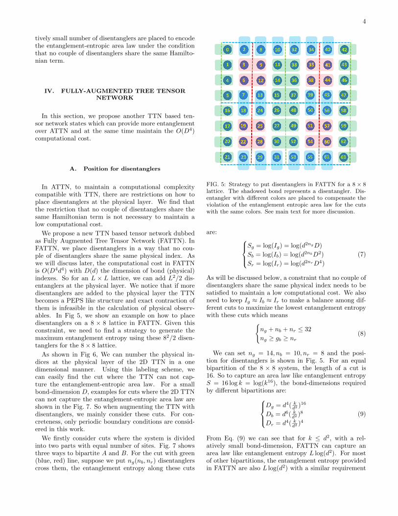
FIG. 5: Strategy to put disentanglers in FATTN for a 8 × 8lattice. The shadowed bond represents a disentangler. Dis-entangler with different colors are placed to compensate theviolation of the entanglement entropic area law for the cutswith the same colors. See main text for more discussion.

are: Sg = log(Ig) = log(d2ngD)

Sb = log(Ib) = log(d2nbD2)

Sr = log(Ir) = log(d2nrD4)

(7)

As will be discussed below, a constraint that no couple ofdisentanglers share the same physical index needs to besatisfied to maintain a low computational cost. We alsoneed to keep Ig ≈ Ib ≈ Ir to make a balance among dif-ferent cuts to maximize the lowest entanglement entropywith these cuts which means{

ng + nb + nr ≤ 32

ng ≥ gb ≥ nr(8)

We can set ng = 14, nb = 10, nr = 8 and the posi-tion for disentanglers is shown in Fig. 5. For an equalbipartition of the 8 × 8 system, the length of a cut is16. So to capture an area law like entanglement entropyS = 16 log k = log(k16), the bond-dimensions requiredby different bipartitions are:

Dg = d4( kd2 )16

Db = d6( kd2 )8

Dr = d4( kd2 )4(9)

From Eq. (9) we can see that for k ≤ d2, with a rel-atively small bond-dimension, FATTN can capture anarea law like entanglement entropy L log(d2). For mostof other bipartitions, the entanglement entropy providedin FATTN are also L log(d2) with a similar requirement

5

0

1

4

5

16

17

20

21

2 8 10 3432 40 42

3 9 11 33 35 41 43

6 12 14 36 38 44 46

7 13 15 3937 45 47

18 24 26 48 50 56 58

19 25 27 49 51 57 59

22 28 30 52 54 60 62

23 29 31 53 55 61 63

0 1 2 63…… 61 62

FIG. 6: Label the physical sites in 2D TTN in a 1D manner.With this we can easily identify the cuts where entanglement-entropic area law is violated.

on D (see the discussion in the Appendix). Comparingwith ATTN, the entanglement entropy in FATTN is dou-bled from L log(d) to L log(d2) on a finite lattice for mostof the cuts with a large D. At the same time the compu-tational cost is O(D4d4) which is comparable to O(D4d2)for ATTN as will be discussed in the next subsection.

B. Optimization of FATTN

To optimize a FATTN, we need to optimize both thedisentanglers and the isometries in it. We follow the pro-cedure in the MERA [35] to optimize disentangler whichis very similar to the optimization of isometry in theTTN. First, we calculate the environment for the disen-tangler we want to optimize. For a Hamiltonian term, wejust need to consider the disentanglers which are directlyconnected to it because other disentanglers can be anni-hilated because of Eq. (6). As show in Fig. 8, we firstlytake a singular value decomposition to get a standardTTN. Then, we contract the TTN to get the environ-ment tensor. This procedure takes a cost of O(D4) asshown in Fig. 9. Once we obtain the environment tensor,we follow the strategy in the TTN to get the optimizeddisentanglers. The details can be found in Fig. 10.

The procedure to optimize isometries is similar. Fora Hamiltonian term, we only need to consider the disen-tanglers which are directly connected to it. We contractthe Hamiltonian term and the connected disentanglers toget an effective Hamiltonian term in same spirit of ATTN

0

1

4

5

16

17

20

21

2 8 10 3432 40 42

3 9 11 33 35 41 43

6 12 14 36 38 44 46

7 13 15 3937 45 47

18 24 26 48 50 56 58

19 25 27 49 51 57 59

22 28 30 52 54 60 62

23 29 31 53 55 61 63

FIG. 7: Examples of cuts where the 2D TTN can not effi-ciently capture the entanglement-entropic area-law are shownin colored dash lines. When placing disentanglers, we need toconsider these cuts to encode the entanglement-entropic arealaw.

(a) (b)

FIG. 8: In the optimization of disentangler, FATTN can bereduced to a TTN like structure with an SVD. Here we onlyshow the disentanglers which are connected with the consid-ered Hamiltonian term.

[43]. We then decompose the partial contracted FATTNinto a sum of a series of standard TTN as shown in theFig. 11. After this, we can follow the procedure in theTTN to optimize the isometries in the FATTN.

Overall, for an arbitrary Hamiltonian term, we decom-pose the relevant disentanglers (for a two-site operator,there are two disentanglers need to be considered in theworst case which causes a factor in the computationalcost of d4). Then, FATTN becomes a standard TTN. Sothe overall computational complexity is O(D4d4).

6

𝑂(𝑑 ) 𝑂(𝑑 )

(a) (b)

(c) (d) (e) (f)

FIG. 9: The computation of the environment for disentan-glers. The cost of this step is O(D4).

E

𝑆𝑉𝐷 𝑈

𝑆

𝑉

V

𝑈

disentangler

(a) (b)

(c) (d)

FIG. 10: The optimization of disentangler from the corre-sponding environment tensor, similar as in Eq. (4).

V. BENCHMARK RESULTS

To show the accuracy of the FATTN, we calculate theground state energy of the transverse Ising model [48]with the Hamiltonian

HIsing = −∑〈i,j〉

σxi σxj − λ

∑i

σzi (10)

where σx and σz are Pauli matrices and λ is the strengthof the transverse magnetic field. We consider a 8 × 8lattice with periodic boundary conditions where highly

(a) (b)

FIG. 11: Similar as in Fig. 8, in the optimization of isometry,FATTN can be reduced to a TTN like structure with an SVD.Here we only show the disentanglers which are connected withthe considered Hamiltonian term.

0.00 0.01 0.02 0.03 0.04 0.051/D

10−5

10−4

10−3

Rel

ativ

eer

ror

TTN

ATTN

1st layer FATTN

2nd layer FATTN

1st and 2nd layer FATTN

FIG. 12: Relative error of the ground state energy for differenttensor network states ansatzes of the transverse Ising modelnear the critical point (λ = 3.05) for a 8 × 8 lattice.

accurate numerical results for energy are available forbenchmark [24]. We focus on λ = 3.05 close to the criticalpoint which is the hard region of this model.

In Fig. 12, we show the relative error of the groundstate energy per site as a function of the bond dimensionat λ = 3.05 for TTN, ATTN, and FATTN. As expected,FATTN gives the lowest energy with fixed D. The errorwith FATTN is reduced by one (a half) order of magni-tude over TTN (ATTN) for all bond dimensions.

The results away from the critical point are shown inFig. 13. We can see a similar improvement of FATTNover TTN and ATTN for λ = 2 and 4.

For lager systems, we do not have accurate results tocompare against. In Fig. 14, we calculate the relativeerror ∆E = |(ED − Eextra)/Eextra| of the ground stateenergy per site for different tensor network ansatzes atdifferent bond-dimension D for a 16 × 16 lattice. Weextrapolate the results calculated by FATTN to obtainEextra. We also find a significant improvement in the

7

0.00 0.01 0.02 0.03 0.04 0.051/D

10−5

10−4

Rel

ativ

eer

ror

TTN

ATTN

1st layer FATTN

0.00 0.01 0.02 0.03 0.04 0.051/D

10−5

10−4

10−3

Rel

ativ

eer

ror

TTN

ATTN

1st layer FATTN

FIG. 13: Relative error of the ground state energy as a func-tion of bond dimension for different tensor network statesansatzes away from the critical point for a 8×8 lattice. Upper:λ = 2. Down: λ = 4.

simulations of FATTN over TTN and ATTN. We noticethat the FATTN result with D = 20 is better than thatof TTN with D = 100. Comparing the 16× 16 results tothe 8×8 results in Fig. 12, we find that the improvementof FATTN over TTN increases with system size.

VI. INTERPOLATION BETWEEN TTN ANDMERA

In the above section, we only place disentanglers at thephysical layer of TTN. But this is not the only scheme toaugment a TTN. We can place disentanglers at any layeror even at multiple layers of the TTN. The key issue isto keep the computational complexity affordable.

A. Single-layer FATTN

The bond dimension of the disentangler depends on itsposition in the TTN which determines the upper boundon the entanglement entropy the FATTN can capture.

0.00 0.01 0.02 0.03 0.04 0.051/D

10−4

10−3

Rel

ativ

eer

ror

TTN

ATTN

1st layer FATTN

FIG. 14: Relative error of the ground state energy for dif-ferent tensor network states ansatzes of the transverse Isingmodel near the critical point (λ = 3.05) for a 16 × 16 lattice,compared with the result extrapolated from FATTN data.

0

2

8

10

1 4 5 1716 20 21

3 6 7 18 19 22 23

9 12 13 24 25 28 29

11 14 15 2726 30 31

FIG. 15: The strategy to place disentanglers in 2nd layerFATTN. Notice that no couple of disentanglers share the samesite to ensure a low computational cost.

If disentanglers are placed at the physical (first) layer ofTTN, the bond dimension of disentangler is d (d = 2 forspin 1/2 system) and the entropy the FATTN can mostlyencode is S = L log(d2).

If we put disentanglers in higher layer, the bond di-mension of disentangler is larger than d (to maintain alow cost, we also need to ensure no couple of disentan-glers share the same site). But a balance between thebond dimension of disentangler and the maximum num-ber of disentanglers can be placed needs to be reached toprovide the maximum entanglement entropy in FATTN.As shown in Fig. 15, we can only place 82/4 disentanglersin the second layer of the TTN, but the bond dimensionof the disentangler becomes d2. So the entanglement en-tropy can be encoded when placing disentanglers in sec-ond layer is the same as the first layer case.

However, when placing disentanglers in higher layer,we find that the entanglement entropy is limited by thered line cuts shown in Fig. 15 or Fig. 5. The entanglemententropy can provide is S = L/4 log(D) if D < d8 (for D >d8, the entanglement entropy the FATTN can provide is

8

Structure Computational Complexity

1st layer O(D4d4)

2nd layer O(D4d8)

3rd layer O(D4d16)

1st & 2nd layer O(D4d20)

ATTN O(D4d2)

TABLE I: The computational complexity for FATTN withdifferent ways to augment the TTN with disentanglers. Theresults for ATTN are also listed for comparison.

still L log(d2)).In TABLE. I, we list the computational complexity for

different types of single-layer FATTN.

B. Multi-layer FATTN

We can also place disentanglers on multiple layers ofthe TTN. It is easily to show that the FATTN is actuallya 2D MERA if disentanglers are placed on every layer ofthe TTN.

2D MERA can provide an area-law entanglement en-tropy proportional to L log(D). But it is highly costlywith a computational complexity O(D16) [33] which lim-its the bond dimension can be reached.

To make a balance between cost and entanglement en-tropy captured in the wave-function ansatz, we can in-terpolate between single layer FATTN and MERA byplacing disentanglers on a relatively small number of lay-ers of the TTN. As an example, we place disentanglersin both the first and second layer of TTN according toFig. 5 and Fig. 15. The computational complexity areshown in Table. I.

C. Results for the single-layer FATTN andmulti-layer FATTN

In Fig. 12, we show the comparison of the relative er-ror of the ground state energy for different tensor net-

work ansatzes. The system is a 8 × 8 transverse Isingmodel with λ = 3.05. The result of 2nd layer FATTNis comparable with 1st layer FATTN, but the 2nd layerFATTN has a higher cost. When placing disentanglerson both the first and second layer, a tiny improvementcan be achieved. From Fig. 12, we can find that the beststrategy for FATTN is to place the disentanglers at thephysical layer according to Fig. 5.

VII. CONCLUSIONS

In this work, we propose a new tensor network stateansatz FATTN by releasing the unnecessary constraintin ATTN. FATTN can provide an area law like entan-glement entropy scaling as L log(d2) for most of the cuts(with a large bond dimension D on a finite lattice) witha low computational cost O(D4d4) if the disentanglersare placed on the physical layer. The benchmark resultson 2D transverse Ising model near critical point show alarge improvement over TTN (nearly one order of mag-nitude) and ATTN (nearly a half order of magnitude) onthe ground state energy. FATTN can be viewed as aninterpolation between TTN and MERA to reach a bal-ance between the computational cost and entanglemententropy captured in the wave-function ansatz. We an-ticipate FATTN will be an efficient practical numericaltool in the future simulation of two dimensional quantummany-body systems on a finite lattice.

Acknowledgments

The calculation in this work is carried out with Quimb[49] and TensorNetwork [50]. This work is supported bya start-up fund from School of Physics and Astronomyin Shanghai Jiao Tong University.

[1] D. C. Cabra, A. Honecker, and P. Pujol, Modern Theoriesof Many-Particle Systems in Condensed Matter Physics,vol. 843 (2012).

[2] W. X. Gang, Quantum field theory of many-body systems:from the origin of sound to an origin of light and electrons(Oxford University Press, Oxford, 2007), URL https:

//cds.cern.ch/record/803748.[3] E. C. Marino, Quantum Field Theory Approach to Con-

densed Matter Physics (Cambridge University Press,2017).

[4] J. P. F. LeBlanc, A. E. Antipov, F. Becca, I. W. Bulik,G. K.-L. Chan, C.-M. Chung, Y. Deng, M. Ferrero, T. M.Henderson, C. A. Jimenez-Hoyos, et al. (Simons Collab-

oration on the Many-Electron Problem), Phys. Rev. X5, 041041 (2015), URL https://link.aps.org/doi/10.

1103/PhysRevX.5.041041.[5] E. Y. Loh, J. E. Gubernatis, R. T. Scalettar, S. R.

White, D. J. Scalapino, and R. L. Sugar, Phys. Rev. B41, 9301 (1990), URL https://link.aps.org/doi/10.

1103/PhysRevB.41.9301.[6] M. Troyer and U.-J. Wiese, Phys. Rev. Lett. 94,

170201 (2005), URL https://link.aps.org/doi/10.

1103/PhysRevLett.94.170201.[7] M. B. Plenio, J. Eisert, J. Dreißig, and M. Cramer, Phys.

Rev. Lett. 94, 060503 (2005), URL https://link.aps.

org/doi/10.1103/PhysRevLett.94.060503.

9

[8] G. Vidal, J. I. Latorre, E. Rico, and A. Kitaev, Phys.Rev. Lett. 90, 227902 (2003), URL https://link.aps.

org/doi/10.1103/PhysRevLett.90.227902.[9] M. Srednicki, Phys. Rev. Lett. 71, 666 (1993), URL

https://link.aps.org/doi/10.1103/PhysRevLett.71.

666.[10] J. Eisert, M. Cramer, and M. B. Plenio, Rev. Mod. Phys.

82, 277 (2010), URL https://link.aps.org/doi/10.

1103/RevModPhys.82.277.[11] P. Silvi, F. Tschirsich, M. Gerster, J. JAŒnemann,

D. Jaschke, M. Rizzi, and S. Montangero, SciPost Phys.Lect. Notes p. 8 (2019), URL https://scipost.org/10.

21468/SciPostPhysLectNotes.8.[12] R. OrAºs, Annals of Physics 349, 117 (2014), ISSN 0003-

4916, URL https://www.sciencedirect.com/science/

article/pii/S0003491614001596.[13] J. C. Bridgeman and C. T. Chubb, Journal of Physics A:

Mathematical and Theoretical 50, 223001 (2017), URLhttps://doi.org/10.1088/1751-8121/aa6dc3.

[14] B.-X. Zheng, C.-M. Chung, P. Corboz,G. Ehlers, M.-P. Qin, R. M. Noack, H. Shi,S. R. White, S. Zhang, and G. K.-L. Chan,Science 358, 1155 (2017), ISSN 0036-8075,http://science.sciencemag.org/content/358/6367/1155.full.pdf,URL http://science.sciencemag.org/content/358/

6367/1155.[15] H. J. Liao, Z. Y. Xie, J. Chen, Z. Y. Liu, H. D. Xie,

R. Z. Huang, B. Normand, and T. Xiang, Phys. Rev.Lett. 118, 137202 (2017), URL https://link.aps.org/

doi/10.1103/PhysRevLett.118.137202.[16] S. R. White, Phys. Rev. B 48, 10345 (1993), URL https:

//link.aps.org/doi/10.1103/PhysRevB.48.10345.[17] S. R. White, Phys. Rev. Lett. 69, 2863 (1992), URL

https://link.aps.org/doi/10.1103/PhysRevLett.69.

2863.[18] U. Schollwoeck and . B. Germany Institute for Advanced

Study Berlin, Wallotstrasse 19, Annals of Physics (NewYork) 326 (2011), ISSN 0003-4916, URL https://www.

osti.gov/biblio/21579838.[19] M. Fannes, B. Nachtergaele, and R. F. Werner, Com-

munications in Mathematical Physics 144, 443 (1992),URL https://doi.org/.

[20] E. Stoudenmire and S. R. White, Annual Re-view of Condensed Matter Physics 3, 111 (2012),https://doi.org/10.1146/annurev-conmatphys-020911-125018, URL https://doi.org/10.1146/

annurev-conmatphys-020911-125018.[21] U. Schollwock, Rev. Mod. Phys. 77, 259 (2005), URL

https://link.aps.org/doi/10.1103/RevModPhys.77.

259.[22] S. Ostlund and S. Rommer, Phys. Rev. Lett. 75,

3537 (1995), URL https://link.aps.org/doi/10.

1103/PhysRevLett.75.3537.[23] U. SchollwA¶ck, Annals of Physics 326, 96 (2011),

ISSN 0003-4916, january 2011 Special Issue, URLhttps://www.sciencedirect.com/science/article/

pii/S0003491610001752.[24] L. Tagliacozzo, G. Evenbly, and G. Vidal, Phys. Rev.

B 80, 235127 (2009), URL https://link.aps.org/doi/

10.1103/PhysRevB.80.235127.[25] Y.-Y. Shi, L.-M. Duan, and G. Vidal, Phys. Rev. A

74, 022320 (2006), URL https://link.aps.org/doi/

10.1103/PhysRevA.74.022320.[26] P. Silvi, V. Giovannetti, S. Montangero, M. Rizzi,

J. I. Cirac, and R. Fazio, Phys. Rev. A 81,062335 (2010), URL https://link.aps.org/doi/10.

1103/PhysRevA.81.062335.[27] M. Gerster, P. Silvi, M. Rizzi, R. Fazio, T. Calarco,

and S. Montangero, Phys. Rev. B 90, 125154 (2014),URL https://link.aps.org/doi/10.1103/PhysRevB.

90.125154.[28] F. Verstraete and J. I. Cirac (2004), cond-mat/0407066.[29] F. Verstraete and J. I. Cirac, Phys. Rev. A 70,

060302 (2004), URL https://link.aps.org/doi/10.

1103/PhysRevA.70.060302.[30] F. Verstraete, M. M. Wolf, D. Perez-Garcia, and

J. I. Cirac, Phys. Rev. Lett. 96, 220601 (2006), URLhttps://link.aps.org/doi/10.1103/PhysRevLett.96.

220601.[31] Z. Y. Xie, J. Chen, J. F. Yu, X. Kong, B. Normand, and

T. Xiang, Phys. Rev. X 4, 011025 (2014), URL https:

//link.aps.org/doi/10.1103/PhysRevX.4.011025.[32] G. Vidal, Phys. Rev. Lett. 101, 110501 (2008), URL

https://link.aps.org/doi/10.1103/PhysRevLett.

101.110501.[33] G. Evenbly and G. Vidal, Phys. Rev. Lett. 102,

180406 (2009), URL https://link.aps.org/doi/10.

1103/PhysRevLett.102.180406.[34] G. Vidal, Phys. Rev. Lett. 99, 220405 (2007), URL

https://link.aps.org/doi/10.1103/PhysRevLett.99.

220405.[35] G. Evenbly and G. Vidal, Phys. Rev. B 79,

144108 (2009), URL https://link.aps.org/doi/10.

1103/PhysRevB.79.144108.[36] S. Liang and H. Pang, Phys. Rev. B 49, 9214 (1994),

URL https://link.aps.org/doi/10.1103/PhysRevB.

49.9214.[37] H. C. Jiang, Z. Y. Weng, and T. Xiang, Phys. Rev. Lett.

101, 090603 (2008), URL https://link.aps.org/doi/

10.1103/PhysRevLett.101.090603.[38] H. Kalis, D. Klagges, R. Orus, and K. P. Schmidt, Phys.

Rev. A 86, 022317 (2012), URL https://link.aps.org/

doi/10.1103/PhysRevA.86.022317.[39] N. Schuch, M. M. Wolf, F. Verstraete, and J. I. Cirac,

Phys. Rev. Lett. 98, 140506 (2007), URL https://link.

aps.org/doi/10.1103/PhysRevLett.98.140506.[40] T. Nishino and K. Okunishi, Journal of the

Physical Society of Japan 65, 891 (1996),https://doi.org/10.1143/JPSJ.65.891, URL https:

//doi.org/10.1143/JPSJ.65.891.[41] Z. Y. Xie, J. Chen, M. P. Qin, J. W. Zhu, L. P. Yang, and

T. Xiang, Phys. Rev. B 86, 045139 (2012), URL https:

//link.aps.org/doi/10.1103/PhysRevB.86.045139.[42] MERA is constructed with isometries and disentanglers

whose definition will be introduced in the main text later.[43] T. Felser, S. Notarnicola, and S. Montangero, Phys. Rev.

Lett. 126, 170603 (2021), URL https://link.aps.org/

doi/10.1103/PhysRevLett.126.170603.[44] A detailed analysis of entanglement entropy of FATTN

can be found in the appendix. There is a requirement onbond dimension D to fulfill the L log(d2) scaling. In thissense, FATTN is designed to study finite systems.

[45] Actually TTN can be constructed from arbitrary rank-3 tensors. But with isometry, the construction becomestrivial.

[46] G. Evenbly and G. Vidal, Algorithms for entanglementrenormalization (2009), 0707.1454.

[47] R. Haghshenas, Phys. Rev. Research 3, 023148

10

0

1

4

5

16

17

20

21

2 8 10 3432 40 42

3 9 11 33 35 41 43

6 12 14 36 38 44 46

7 13 15 3937 45 47

18 24 26 48 50 56 58

19 25 27 49 51 57 59

22 28 30 52 54 60 62

23 29 31 53 55 61 63

0

1

4

5

16

17

20

21

2 8 10 3432 40 42

3 9 11 33 35 41 43

6 12 14 36 38 44 46

7 13 15 3937 45 47

18 24 26 48 50 56 58

19 25 27 49 51 57 59

22 28 30 52 54 60 62

23 29 31 53 55 61 63

FIG. 16: Two cuts for a 8 × 8 lattice which is not discussedin the main text. There is no disentangler across these cutsin FATTN.

(2021), URL https://link.aps.org/doi/10.1103/

PhysRevResearch.3.023148.[48] S. Suzuki, J.-i. Inoue, and B. K. Chakrabarti, Intro-

duction (Springer Berlin Heidelberg, Berlin, Heidelberg,2013), pp. 1–11, ISBN 978-3-642-33039-1, URL https:

//doi.org/10.1007/978-3-642-33039-1_1.[49] J. Gray, Journal of Open Source Software 3, 819 (2018).[50] C. Roberts, A. Milsted, M. Ganahl, A. Zalcman,

B. Fontaine, Y. Zou, J. Hidary, G. Vidal, and S. Le-ichenauer, Tensornetwork: A library for physics and ma-chine learning (2019), 1905.01330.

Appendix A: The entanglement entropy of FATTN

In this section, we give a detailed analysis on the en-tanglement entropy the FATTN can encode. In the maintext, we show that the entanglement entropy along thecolored dash line in the Fig. 5 is L log(d2). And the re-quirements for the bond-dimension to encode the entropyof L log(k) along the colored boundaries are:

Dg = d4( kd2 )16

Db = d6( kd2 )8

Dr = d4( kd2 )4(A1)

Now, we will show that if these conditions are satisfied,the requirements for most of the other cuts will be alsosatisfied.

We firstly consider a 8 × 8 lattice. For the black areashown in the upper panel of Fig. 16 where we do notplace any disentangler. The boundary length of the cutis 20. So in order to encode an entropy of log(k20) therequirement is:

k20 = D4d20 → D = d5(k

d2)5 (A2)

So once again, we need k ≤ d2 if we want to use a smallbond-dimension D to encode the entanglement-entropicarea law of L log(d2).

For the bipartition shown in the down panel of Fig. 16,the requirement is:

k16 = D2d16 → D = d8(k

d2)8 (A3)

We still need k ≤ d2 if we want to use a small bond-dimension D to encode the entanglement-entropic arealaw of L log(d2). For other cuts whose boundary issmaller or there are disentanglers across them, the re-quirement is also satisfied. So, the FATTN can efficientlyencode an entanglement-entropic area law of L log(d2) fora 8× 8 lattice.

We can iteratively use the strategies for 8 × 8 latticeshown in Fig. 5 to analyze larger lattices. In Fig. 17, we

0

1

4

5

16

17

20

21

2 8 10 3432 40 42

3 9 11 33 35 41 43

6 12 14 36 38 44 46

7 13 15 3937 45 47

18 24 26 48 50 56 58

19 25 27 49 51 57 59

22 28 30 52 54 60 62

23 29 31 53 55 61 63

0

1

4

5

16

17

20

21

2 8 10 3432 40 42

3 9 11 33 35 41 43

6 12 14 36 38 44 46

7 13 15 3937 45 47

18 24 26 48 50 56 58

19 25 27 49 51 57 59

22 28 30 52 54 60 62

23 29 31 53 55 61 63

FIG. 17: The way to place disentanglers of FATTN on a 8×16lattice following the strategy in 8 × 8 lattice in Fig. 5. Thisstrategy can be repeated for the placement of disentanglersin FATTN for larger systems.

11

take a 16 × 8 lattice as an example. For a general finitesystem, the requirement of an area law as L log(k) is

kL = DL/cdLdpL → D = dc(1−p)(k/d2)c (A4)

where pL(p ∈ [0, 1]) is the number of disentanglers acrossthe cut and c is a cut dependent constant. Because weplace disentanglers across the cuts where c is large, which

means p is close to 1 if c is large. So for most of the cutsc(1 − p) is relatively small which means for these cutthe captured entanglement entropy scales L log(d2). Wecan also increase the dimension of the relevant bonds forthese cuts with large c(1 − p) but maintain a relativelysmall D for other bonds.