From TV-L1 Model to Convex & Fast Optimization Modelsfor Image & Geometry Processing

Tony Chan, UCLA and NSF

Joint work with Xavier Bresson, UCLA

Papers: www.math.ucla.edu/applied/cam/index.htmlResearch group: www.math.ucla.edu/∼imagers

May 28, 2009

Outline

The ”classical” TV-L2 model introduced by Rudin, Osher and Fatemi1 is anefficient image denoising model. However, TV-L2 does not preserve imagecontrast unlike the TV-L1 model introduced by Chan and Esedoglu2 .

The TV-L1 model also leads to the convexification of several non-convex imageprocessing models.

Standard models are defined by non-convex energy minimization problems, whichmake them sensitive to initial conditions and slow to minimize. We show how toconvexify standard image processing models and how to define fast optimizationalgorithms.

Applications to Image Processing and Computer Vision: Image Segmentation,Multiview 3D Reconstruction, Stereo Evaluation, Optical Flow & ObjectTracking, Multi-phase Segmentation, etc.

1Rudin-Osher-Fatemi, Nonlinear Total Variation Based Noise Removal Algorithms, 1992

2Chan-Esedoglu, Aspects of Total Variation Regularized L1 Function Approximation, 2005

2 / 26

Image Denoising: TV-L2 Model (Rudin-Osher-Fatemi/ROF 92)

The Total Variation (TV) norm has been successful in Image Processing. TheTV-based ROF model defined as an energy minimization/variational model:

minu,u−u0∈BV (Ω)×L2(Ω)

TV (u) +λ

2||u − u0||

22,

where TV (u) =

∫

Ω|∇u|dx

removes the noise in u0 while preserving discontinuities (edges).

TV is important because:

• TV controls the size of jumps in signal since for u monotonic in [a, b], thenTV (u) = |u(b) − u(a)|, regardless of whether u is discontinuous or not. TV canhandle image discontinuities.

• TV also controls the geometry of boundary since for the characteristic function1Σ of region Σ ⊂ Ω since we have: TV (u = 1Σ) =

∫

∂Σ ds = |∂Σ| = Per(∂Σ).

3 / 26

TV-L1 Model: Contrast & Geometry Preservation (Alliney 97,Chan-Esedoglu 05)

The ROF image denoising model preserves the geometry in the presence of noise.However, ROF loses the image contrast (Strong-Chan 96, Bellettini-Caselles-Novaga 02).Theorem: If u0 = 1D , D is convex, ∂D ∈ C1,1 and for every p ∈ ∂D,

curv∂D (p) ≤ |∂D||D|

, then

u =(

1 −|∂D|

2λ|D|︸ ︷︷ ︸

Contrast Lost

)

1D

The TV-L1 energy minimization model:

minu,u−u0∈BV (Ω)×L1(Ω)

TV (u) + λ||u − u0||1,

• is robust to contrast and geometry perturbation in the presence of noise• does not perturb a clean image in the absence of noise

Other properties of TV-L1 Model:

• Cleaner image multiscale decomposition than ROF

• Data driven scale selection (detection of meaningful objects in images)

• Shape denoising/Geometry regularization model

4 / 26

Scale-Space Generated by the ROF Model and the TV-L1 Model

(a) ROF (b) TV-L1

5 / 26

Multiscale Decomposition of TV-L1 (Related: Tadmor-Nezzar-Vese 03;Kunisch-Scherzer 03)

Figure: TV-L1 decomposition gives well separated & contrast preserving features at differentscales. E.g. boat masts, foreground boat appear mostly in only 1 scale.

6 / 26

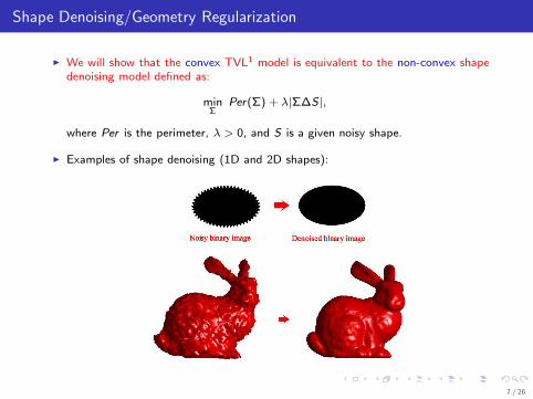
Shape Denoising/Geometry Regularization

We will show that the convex TVL1 model is equivalent to the non-convex shapedenoising model defined as:

minΣ

Per(Σ) + λ|Σ∆S|,

where Per is the perimeter, λ > 0, and S is a given noisy shape.

Examples of shape denoising (1D and 2D shapes):

7 / 26

Equivalence between TV-L1 Model and Shape Denoising

In the case of Shape Denoising, function u0 is a binary function of the (noisy)shape D:

u0(x) = 1D (x) =

1 if x ∈ D

0 otherwise

The co-area formula decomposes TV into the sum of Perimeters of level sets of u:

TV (u) =

∫

Ω|∇u|dx =

∫

µ

Per(x : u(x) > µ︸ ︷︷ ︸

Σ(µ)

)dµ.

The ”Layer Cake” formula decomposes the L1-based data term as follows:∫

Ω|u − u0|dx =

∫

µ

|Σ(µ)∆x : u0(x) > µ|dµ.

With u0 = 1D , we have

TVL1(u) =

∫

µ

Per(Σ(µ)) + λ|Σ(µ)∆D|dµ.

which means that, for each upper level set of u(x), we have the same geometryproblem:

minΣ

Per(Σ) + λ|Σ∆D|

8 / 26

TVL1 provides a Global Minimizer of the Shape Regularization Problem

(Chan-Esedoglu-Nikolova 053)

Theorem: If the observed image u0(x) is the (noisy) binary function of a set D

and if u⋆ is any minimizer of TVL1, then for almost every µ ∈ (0, 1), the binaryfunction 1x :u⋆(x)>µ(x) is also a minimizer of TVL1.

TVL1 has ”convexified” the shape regularization problem! In other words, wehave established the equivalence of a convex problem (minimizing over allfunctions) to a non-convex problem (minimizing over geometric sets).

3Chan-Esedoglu-Nikolova, Algorithms for Finding Global Minimizers of Image Segmentation and Denoising Models, 2006

9 / 26

Image Segmentation: Active Contour Models

Image segmentation consists in partitioning an image into multiple regions.Image segmentation locates meaningful objects in images. Applications are invideo surveillance, medical imaging, etc.

A well-posed mathematical model is the active contour model(Kass-Witkin-Terzopoulos 88). Objective: Find the set Σ ⊂ Ω ⊂ R

N whichprovides the global minimum of the shape optimization problem:

minΣ

FAC (Σ) =

∫

∂Σwbds

︸ ︷︷ ︸

Perwb(Σ)

+λ

∫

Σw in

r dx

︸ ︷︷ ︸

Areawin

r(Σ)

+λ

∫

Ω\Σwout

r dx

︸ ︷︷ ︸

Areawoutr

(Ω\Σ)

. (1)

The shape model (1) is not convex becausethe set of Σ and the energy FAC are not convex.

10 / 26

Connection of Active Contours to TV

The convex TV-〈, 〉 energy defined as:

FTV 〈,〉(u) =

∫

Ωwb|∇u|dx

︸ ︷︷ ︸

TVwb(u)

+λ

∫

Ωw in

r udx

︸ ︷︷ ︸

<w inr ,u>

+λ

∫

Ωwout

r (1 − u)dx

︸ ︷︷ ︸

<woutr ,1−u>

can be decomposed into a sum of upper level set energies (using weighted co-areaformula and layer-cake formula):

FTV 〈,〉(u) =

∫

µ

Perwb(Σ(µ)) + λAreaw in

r(Σ(µ)) + λAreawout

r(Ω \ Σ(µ)) dµ

which means that, for each upper level set of u(x), we have the same geometryproblem:

minΣ

Perwb(Σ) + λAreawr (Σ) + λAreawout

r(Ω \ Σ) = FAC (Σ)

which corresponds to the non-convex active contour minimization problem.

11 / 26

TV-〈, 〉 provides a Global Minimizer of the Active Contour Problem(Chan-etal 06, Bresson-etal 07)

Theorem: Suppose that wb(x) ∈ R+, for any fixed w inr (x), wout

r (x) ∈ R andλ ∈ R+, if u⋆ is any minimizer of min0≤u≤1 FTV 〈,〉(u), then for almost everyµ ∈ (0, 1), the binary function 1x :u⋆(x)>µ(x) is also a global minimizer ofFTV 〈,〉 and the active contour energy FAC .

TV-〈, 〉 has convexified the image segmentation problem!

The non-convex Chan-Vese model:

minΣ

FCV (Σ) = Per(Σ) + λ

∫

Σ(c in − u0)

2dx + λ

∫

Ω\Σ(cout − u0)

2dx ,

can be convexified as follows:

min0≤u≤1

F cCV (u) =

∫

Ω|∇u|dx + λ

∫

Ω(c in − u0)

2udx + λ

∫

Ω(cout − u0)

2(1 − u)dx

If u⋆ is any minimizer of F cCV

, then the binary function 1x :u⋆(x)>µ(x) is aglobal minimizer of FCV .

12 / 26

Optimization Algorithm for the TV-〈, 〉 Segmentation Model

What optimization algorithm for TV-〈, 〉? Standard algorithms for continuousenergy minimization problems were usually slow to converge because they arenon-convex (and non-differentiable).Since TV-〈, 〉 is convex, we can use efficient optimization techniques (that canlead to real-time applications).

Rich literature on continuous convex optimization algorithms: Rockafellar 76(Proximal Point Algorithm), Hestenes 69, Powell 69 (Method of Multipliers/Augmented Lagrangian), Passty 79, Gabay 83, Tseng 88 (Forward-Backward),Lions 1978, Passty 79 (Double-Backward), Lions and Mercier 79(Peaceman-Rachford), Lions and Mercier 79 (Douglas-Rachford).There has been a new interest for these optimization models to solve the problemof compressive sensing of Candes-Romberg-Tao 06, for examplesYin-Osher-Goldfarb-Darbon 08, Goldstein-Osher 08, Zhang-Burger-Bresson-Osher09.

We define an efficient algorithm based on Bregman Iteration (which is a specialcase of Augmented Lagrangian method and Douglas-Rachford algorithm) tominimize TV-〈, 〉.

13 / 26

The TV-〈, 〉 Segmentation Model is Non-Differentiable

The TV-〈, 〉 minimization problem:

min0≤u≤1

FTV 〈,〉(u) =

∫

Ωwb|∇u|dx + λ < w in

r , u > +λ < woutr , (1 − u) >

︸ ︷︷ ︸

λ<wr ,u>+Cte, wr :=w inr −wout

r

is difficult to solve because TV is non-differentiable. Wang-Yin-Zhang 07 andGoldstein-Osher 08 have recently proposed a splitting approach to overcome thisissue in the context of denoising and Compressed Sensing.

The original unconstrained minimization problem is replaced by the constrainedminimization problem:

minu∈[0,1], d∈R2

∫

Ωwb|d|dx

︸ ︷︷ ︸

|d|wb

+λ < wr , u > such that d = ∇u,

and relaxed to this unconstrained minimization problem:

minu,d

|d|wb+ λ < wr , u >

︸ ︷︷ ︸

F (u,d)

+ρ

2

∫

Ω|d −∇u|2

︸ ︷︷ ︸

||d−∇u||2

.

How to enforce the constraint? Wang-Yin-Zhang used the continuation principle,i.e. ρk → ∞.

14 / 26

Split-Bregman Iteration: An Alternative of the Continuation Principle(Goldstein-Osher 08, Goldstein-Bresson-Osher 09)

The Split-Bregman iteration method allows to exactly enforce the constraintd = ∇u during the minimization process.

The core of this method is the ”Bregman Distance” of the (convex) functionalF (u, d):

DF (u, d, uk , dk , pku , pk

d ) = F (u, d)− < pku , u − uk > − < pk

d , d − dk >,

where pu , pd are the subgradient of F w.r.t. u, d.

It can be shown that the following iterative process:

(uk+1, dk+1) = arg minu∈[0,1],d DF (u, d, uk , dk , pku , pk

d) + ρ

2||d −∇u||2

pk+1u = pk

u − ρdiv(dk+1 −∇uk+1)

pk+1d

= pkd− ρ(dk+1 −∇uk+1)

holds the following properties:• ||dk −∇uk || → 0 as k → ∞• The limit u⋆ := limk→∞ uk satisfies the original constrained problem:

u⋆ := arg min0≤u≤1

FTV 〈,〉(u)

15 / 26

Split-Bregman = Augmented Lagrangian (Glowinski-Le Tallec 89, Setzer09)

The Split-Bregman iterative process can be re-written as an AugmentedLagrangian algorithm:

(uk+1, dk+1) = arg min0≤u≤1,d F (u, d)+ < bk ,∇u − d > + ρ2||∇u − d||2

bk+1 = bk + ∇uk+1 − dk+1

It can also be shown that the Alternating Split-Bregman (ASB) iterative process:

uk+1 = arg min0≤u≤1 F (u, dk )+ < bk ,∇u − dk > + ρ2||∇u − dk ||2

dk+1 = arg mind F (uk+1, d)+ < bk ,∇uk+1 − d > + ρ2||∇uk+1 − d||2

bk+1 = bk + ∇uk+1 − dk+1

is equivalent to a Douglas-Rachford Splitting (DRS) Algorithm on the dual.

Proof: Minimization problems like:

minu

J(u) + H(u) ⇔ −minp

J⋆(p) + H⋆(p)

satisfies the Karush-Kuhn-Tucker conditions: 0 ∈ A(p) + B(p). The solution p

can be computed with the DRS algorithm:

tk+1 = ProxηA(I − ηB)pk + ηBpk

pk+1 = ProxηB (tk+1)

Finally, ASB is equivalent to DRS for A = ∂(<, >⋆ o (−div)), B = ∂(||)⋆ andη = ρ.

16 / 26

Comparison with Graph-Cuts

The TV-〈, 〉 model can be optimized with Graph-Cuts (parametric max flow/mincut, Ford-Fulkerson 62). Graph-Cuts is a combinatorial technique that exactlyoptimizes binary energies (which fits well for our problem). This optimizationmethod is fast (Boykov-Kolmogorov 04). Graph-Cuts have also some limitations.This technique:• uses anisotropic schemes to approximate the length (it cannot produce curvedlines)• is pixel accurate• has memory limitations for 3D data• is not easily parallelized• and its speed depend on spatial connectivity.

The proposed continuous optimization algorithm for TV-〈, 〉:• is faster than Graph-Cuts (much faster than Level Set Method).• uses isotropic schemes• is sub-pixel accurate• has low memory usage for 3D data• is easy to parallelize• requires a stopping criterion.

17 / 26

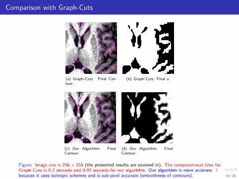
Comparison with Graph-Cuts

(a) Graph-Cuts. Final Con-tour.

(b) Graph-Cuts. Final u.

(c) Our Algorithm. FinalContour.

(d) Our Algorithm. FinalContour.

Figure: Image size is 256 × 256 (the presented results are zoomed in). The computational time forGraph-Cuts is 0.2 seconds and 0.07 seconds for our algorithm. Our algorithm is more accuratebecause it uses isotropic schemes and is sub-pixel accurate (smoothness of contours). 18 / 26

Convex Segmentation/Classification Models in High-Dimensional Spaces

(Bresson-Chan 089)

We extend the continuous model TV-〈, 〉 to work in high-dimensional spaces.Main advantage: segmentation/classification process for any data representation(image intensity, image patch, image, etc).Representation: the high-dimensional data (point in R

n) are represented by thevertices of a graph.Applications: Interactive Segmentation, Machine Learning, etc.

Related works: growing interest to develop PDEs/Wavelets on graph. Forexamples Coifman-Maggioni4, Szlam-Maggioni-Coifman5, Zhou-Scholkopf6 ,Gilboa-Osher7, Jones-Maggioni-Schul8 , etc.

4Coifman-Maggioni, Diffusion wavelets, 2006

5Szlam-Maggioni-Coifman, Regularization on Graphs with Function Adapted Diffusion Processes, 2008

6Zhou-Scholkopf, A Regularization Framework for Learning from Graph Data, 2004

7Gilboa-Osher, Nonlocal linear image regularization and supervised segmentation, 2007

8Jones-Maggioni-Schul, Universal Local Parametrizations via Heat Kernels and Eigenfunctions of the Laplacian, 2007

9Bresson-Chan, Non-local Unsupervised Variational Image Segmentation Models, 2008

19 / 26

TV-〈, 〉 on Graph

The extended TV-〈, 〉 on graph is:

min0≤u≤1

∑

Ω

wb|∇Gu| + λ < wr , u >

where the domain Ω can be the standard image domain, but more generally theset of all vertices of the conidered graph (vertices can belong to high-dimensionalspace).

TV on graph10 ,11,12:

TVG(u) =∑

Ω

|∇Gu|,

where the gradient operator on graph ∇G is defined for a pair of points (x , y) inthe domain Ω as:

∇Gu(x , y) := (u(y) − u(x))√

w(x , y) : Ω × Ω → R,

where w(x , y) is the edge function of the graph G between vertices x and y .

10Chan-Osher-Shen, The digital TV filter and nonlinear denoising, 2001

11Zhou-Scholkopf, A Regularization Framework for Learning from Graph Data, 2004

12Gilboa-Osher, Nonlocal linear image regularization and supervised segmentation, 2007

20 / 26

Global Minimization Theorem

Can we extend the global minimization theorem to graph? Not directly since thecoarea formula does not exist on graph. However, if we assume that the set ofpoints/vertices of the graph belong to a submanifold M of R

n, where thedimension of M is much smaller that the ambient space d < n 13, then we canshow14,15:

∑

Ω

1

ǫd+2

4

|∇Gǫu| →

ǫ→0

∫

M|∇Mu|,

with the graph Gǫ defined with wǫ(x , y) = exp(

−||x − y ||2

ǫ

)

Using the co-area formula on manifold (which exists), the global minimizationtheorem can be extended. In other words, to extract a global minimizer, we needto compute the minimizer of TVG-〈, 〉 and threshold it.

13Belkin, Problems of Learning on Manifolds, 2003

14Bresson-Chan, Non-local Unsupervised Variational Image Segmentation Models, 2008

15Coifman-Lafon, Diffusion maps, 2006

21 / 26

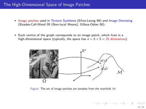
The High-Dimensional Space of Image Patches

Image patches used in Texture Synthesis (Efros-Leung 99) and Image Denoising(Buades-Coll-Morel 05 (Non-local Means), Gilboa-Osher 08).

Each vertice of the graph corresponds to an image patch, which lives in ahigh-dimensional space (typically, the space has n = 5 × 5 = 25 dimensions).

Figure: The set of image patches are samples from the manifold M

22 / 26

Unsupervised Segmentation: Chan-Vese Model in the High-DimensionalSpace of Image Patches (Bresson-Chan 08)

Chan-Vese on the space/graph of image patches:

min0≤u≤1

∑

Ω

|∇Gu| + λ < wr , u >

with wr = (c in − u0)2 − (cout − u0)

2

and w(x , y) = exp(

−||p(x) − p(y)||2

h

)

,

where p(.) is the patch at x .

The original CV model is limited to segment small structures because standardTV decreases the length of iso level sets. In the case of TV defined on the graphof image patches, the new CV model is able to denoise and preserve smallstructures which are repetitive (which is often the case in natural images).

23 / 26

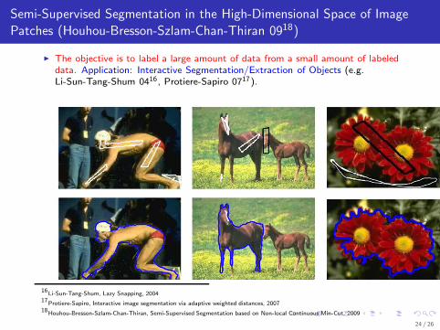
Semi-Supervised Segmentation in the High-Dimensional Space of Image

Patches (Houhou-Bresson-Szlam-Chan-Thiran 0918)

The objective is to label a large amount of data from a small amount of labeleddata. Application: Interactive Segmentation/Extraction of Objects (e.g.Li-Sun-Tang-Shum 0416, Protiere-Sapiro 0717).

16Li-Sun-Tang-Shum, Lazy Snapping, 2004

17Protiere-Sapiro, Interactive image segmentation via adaptive weighted distances, 2007

18Houhou-Bresson-Szlam-Chan-Thiran, Semi-Supervised Segmentation based on Non-local Continuous Min-Cut, 2009

24 / 26

Semi-supervised classification/ Machine Learning in the High-DimensionalSpace of Images (On-Going Work)

Chan-Vese (CV) in the space of images for semi-supervised classification.Connection to K-means: The data term of CV corresponds to a 2-meansalgorithm. The main advantage of CV over K-means is the TV regularizationterm (CV is a better classification method).

The extended CV model to K-means can be applied to Machine Learning.Application: classification of digit numbers using the MNIST database ofhandwritten digits (training set of 60,000 examples).

Figure: A cloud of points represents the numbers 0,...,9 projected on a 3D space with PCA.

25 / 26

Conclusion

The convexification approach introduced with TV-L1 and TV-〈, 〉 models havebeen used to convexify Image Processing and Computer Vision problems such asMultiview 3D Reconstruction19 , Stereo Evaluation20, Optical Flow & ObjectTracking21 , Multi-phase Segmentation22 , etc.

Standard non-convex image processing problems have been reformulated asconvex optimization problems, which are guaranteed to provide the globalminimizing solution (independently of the initial condition). Besides, convexoptimization problems can benefit from fast continuous optimization algorithmsborrowed from Operator Splitting techniques.

19Kolev-Klodt-Brox-Esedoglu-Cremers, Continuous global optimization in multiview 3d reconstruction, 2007

20Pock-Schoenemann-Cremers-Bischof, A convex formulation of continuous multi-label problems, 2008

21Zach-Pock-Bischof, A Duality Based Approach for Realtime TV-L1 Optical Flow, 2007

22Chambolle-Pock-Cremers-Bischof, A Convex Relaxation Approach for Computing Minimal Partitions, 2009

26 / 26