From XML Schema to Relations:

A Cost-Based Approach to XML Storage

Phil Bohannon Juliana Freire Prasan Roy Jerome Simeon

Bell Labs�bohannon,juliana,prasan,simeon � @research.bell-labs.com

Abstract

XML has become an important medium for data representation, particularly when that data is ex-

changed over or browsed on the Internet. As the volume of XML data increases, there is a growing

interest in storing XML in relational databases so that the well-developed features of these systems (e.g.,

concurrency control, crash recovery, query processors) can be re-used. However, given the wide variety

of XML applications and the mismatch between XML’s nested-tree structure and the flat tuples of the

relational model, storing XML documents in relational databases presents interesting challenges.

LegoDB is a cost-based XML-to-relational mapping engine that addresses this problem. It explores

a space of possible mappings and selects the best mapping for a given application (defined by an XML

Schema, XML data statistics, and an XML query workload). LegoDB leverages existing XML and

relational technologies: it represents the target application using XML standards and constructs the space

of configurations using XML-specific operations, and it uses a traditional relational optimizer to obtain

accurate cost estimates of the derived configurations. In this paper, we describe the LegoDB mapping

engine and provide experimental results that demonstrate the effectiveness of this approach.

1 Introduction

As XML is now an important medium for representing, exchanging and accessing data over the Internet,

applications are processing an increasing amount of XML data. Not surprisingly, there is a growing interest

in storing XML in relational databases so that these applications can use a complete set of data management

services (including concurrency control, crash recovery, scalability, etc) and benefit from the highly opti-

mized relational query processors. A number of strategies have been proposed [7, 11, 14, 18, 19] to address

the XML-to-relational mapping problem. An important limitation of most of these proposals is that they rely

on a fixed XML-to-relational mapping. One single mapping is unlikely to work well for more than a few of

the wide variety of access patterns an application may present. For example, a web site may perform a large

volume of simple lookup queries, whereas a catalog printing application may require large and complex

queries with deeply nested results. Modern commercial databases (see e.g., [24]), on the other hand, provide

a more flexible approach to storing XML data, by allowing the developer to specify the storage mapping.

1

However, this approach has drawbacks, most notably: it requires the developer to master two quite distinct

technologies (XML and RDBMS); and it might be hard, even for an expert, to determine a good mapping

for a complex application.

In this paper, we introduce a novel cost-based framework for XML-to-relational storage mapping, and

describe the design of LegoDB, a tool based on this framework that automatically finds an efficient XML-to-

relational mapping for a target application. The three main design principles behind LegoDB are cost-based

search, logical/physical independence, and re-use of existing technology. Since the effectiveness of one-

size-fits-all mapping is improbable given the wide variety of XML applications (with data ranging from flat

to nested, schemas ranging from structured to semistructured, access patterns ranging from traditional SPJ

queries to full-text or recursive queries), our first principle is to take application parameters into account.

More precisely, given a schema describing the XML data to be processed, a query workload, and data

statistics, the LegoDB engine explores various relational configurations in order to find the most efficient

for the application.

Our second principle is to support logical/physical independence. Developers of XML applications

should deal with XML structures and operations and they should not be concerned with the underlying

physical storage in a relational database. Hence, the LegoDB interface is purely XML-based—it takes as

input XML queries, schemas and statistics.

Our third principle is to leverage existing XML and relational technology whenever possible. LegoDB

relies on: 1) existing XML standards to represent the target application, 2) XML-specific operations over a

schema to generate a space of possible mappings, and 3) a traditional relational optimizer to obtain accurate

cost estimates for the derived mappings. On the first point, queries which make up the application workload

are given in XQuery [5], and the user data is described with XML Schema [21].

Our main contributions are summarized below.

� We introduce the notion of physical XML Schemas (p-schemas), which are XML Schemas extended with

statistics about the underlying XML data. We define a fixed mapping from a particular p-schema to a

relational schema and a corresponding mapping from XML documents to databases.

� We define XML Schema transformations that when applied to a p-schema and followed by the fixed map-

ping, lead to a space of alternative storage configurations. The idea is that one may define many alternate

XML Schemas which are equivalent in terms of the documents which are valid under each schema, but

yield different configurations. For instance, types can be introduced or elided, and regular expressions can

be rewritten without affecting the semantics of the schema. Because the proposed rewritings are specific

to XML Schema, this search space contains many configurations not exploited by relational storage design

tools (see, for example, [1, 23]).

� Through the fixed mapping, XML-specific statistics are translated into the corresponding relational statis-

tics, and XQuery workloads are converted into the corresponding SQL workloads. As a result, we can

exploit a traditional relational optimizer to obtain cost estimates for the various configurations, and select

the best among them. One potential problem with this approach is search space explosion. Due to the nature

2

of XML Schema, the schema transformations may lead to a large (possibly infinite) search space. In this

paper we use a greedy evaluation strategy to explore an interesting subset of this space.

� We give experimental results which show that LegoDB is able to find efficient storage designs for a variety

of workloads in a reasonable time. Our results indicate that our cost-based exploration selects storage

designs which would not be arrived at by previously-proposed heuristics, and that in most cases, these

designs have significantly lower costs.

Organization of the Paper The rest of the paper is organized as follows. In Section 2, we present a moti-

vating example along with some background information. In Section 3, we present the LegoDB framework

for mapping XML Schemas, queries, and documents into relational configurations, queries, and databases.

In Section 4, we present the rewriting rules defining the search space and our search algorithm. In Section 5,

we present preliminary experimental results. We review related work in Section 6, and discuss directions

for future work in Section 7.

2 Background and Motivating Example

In this section, we motivate our approach, notably the use of XML Schema and the cost-based evaluation

of storage mappings, with an example XML storage mapping scenario inspired from the Internet Movie

Database [13].

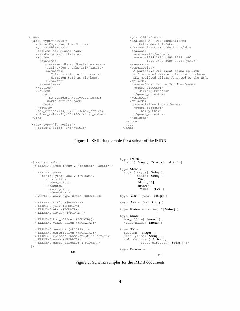
XML documents and DTDs Figure 1 gives an example XML fragment in which the show element is

used to represent movies and TV shows. This element contains information that is shared between movies

and TV shows, such as title and year as well as information specific to movies (e.g., box office

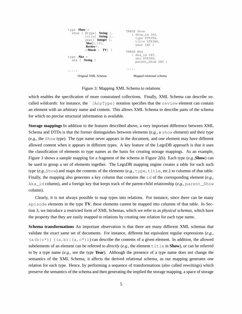
and video sales) and to TV shows (e.g., seasons). Figure 2(a) shows a Document Type Definition

(DTD) [2] for the example document of Figure 1. The DTD contains declarations for all elements and

attributes in the document. The contents of each element may be text (e.g., #PCDATA, CDATA), or a regular

expression over other elements (e.g., (show*,director*,actor*)).

Using XML Schema for storage Figure 2(b) shows an alternative schema described using the notation

for types from the XML Query Algebra [9]. This notation captures the core semantics of XML Schema,

abstracting away some of the complex features of XML Schema which are not relevant for our purposes

(e.g., the distinction between groups and complexTypes, local vs. global declarations, etc). The XML

Schema and the XML Query Algebra notation for our sample schema can be found in Appendix B.

Like DTDs, XML Schema describes elements (e.g., show) and attributes (e.g., @type) and uses reg-

ular expressions to describe allowed subelements (e.g., imdb contains Show*, Director*, Actor*). But

Figure 2(b) also illustrates a number of distinguishing features that are useful for storage. First, one can

specify precise data types (e.g., String, Integer) instead of text, an essential feature for generating an

efficient storage configuration. Also, regular expressions are extended with more precise cardinality anno-

tations for collections (e.g.,�1,10 � indicates that there can be between 1 to 10 aka elements for show),

3

<imdb><show type="Movie"><title>Fugitive, The</title><year>1993</year><aka>Auf der Flucht</aka><aka>Fuggitivo, Il</aka><review><suntimes>

<reviewer>Roger Ebert</reviewer><rating>Two thumbs up!</rating><comments>

This is a fun action movie,Harrison Ford at his best.

</comment></suntimes>

</review><review>

<nyt>The standard Hollywood summermovie strikes back.

</nyt></review><box_office>183,752,965</box_office><video_sales>72,450,220</video_sales>

</show>

<show type="TV series"><title>X Files, The</title>

<year>1994</year><aka>Akte X - Die unheimlichen

Falle des FBI</aka><aka>Aux frontieres du Reel</aka><seasons>

<number>10</number><years>1993 1994 1995 1996 1997

1998 1999 2000 2001</years></seasons><description>

A paranoiac FBI agent teams up witha frustrated female scientist to chaseDNA modified aliens financed by the NSA.

<episode><name>Ghost in the Machine</name><guest_director>

Jerrold Freedman</guest_director>

</episode><episode>

<name>Fallen Angel</name><guest_director>

Larry Shaw</guest_director>

</episode></show>....

</imdb>

Figure 1: XML data sample for a subset of the IMDB

<!DOCTYPE imdb [<!ELEMENT imdb (show*, director*, actor*)>

<!ELEMENT show(title, year, aka+, reviews*,

((box_office,video_sales)

|(seasons,description,episode*)))>

<!ATTLIST show type CDATA #REQUIRED>

<!ELEMENT title (#PCDATA)><!ELEMENT year (#PCDATA)><!ELEMENT aka (#PCDATA)><!ELEMENT review (#PCDATA)>

<!ELEMENT box_office (#PCDATA))><!ELEMENT video_sales (#PCDATA))>

<!ELEMENT seasons (#PCDATA))><!ELEMENT description (#PCDATA))><!ELEMENT episode (name,guest_director)><!ELEMENT name (#PCDATA)><!ELEMENT guest_director (#PCDATA)>

]>

(a)

type IMDB =imdb [ Show*, Director*, Actor* ]

type Show =show [ @type[ String ],

title[ String ],Year,Aka

�1,10 � ,

Review*,( Movie | TV) ]

type Year = year[ Integer ]

type Aka = aka[ String ]

type Review = review[ ˜ [ String ] ]

type Movie =box_office[ Integer ],video_sales[ Integer ]

type TV =seasons[ Integer ],description[ String ],episode[ name[ String ],

guest_director[ String ] ]*

type Director = ...

(b)

Figure 2: Schema samples for the IMDB documents

4

type Show =show [ @type[ String ],

title[ String ],year[ Integer ],Aka

�1,10 � ,

Review*,( Movie | TV) ]

type Aka =aka [ String ]

.....

TABLE Show( Show_id INT,

type STRING,title STRING,year INT )

TABLE Aka( Aka_id INT,

aka STRING,parent_Show INT )

.....

Original XML Schema Mapped relational schema

Figure 3: Mapping XML Schema to relations

which enables the specification of more constrained collections. Finally, XML Schema can describe so-

called wildcards: for instance, the�

[AnyType] notation specifies that the review element can contain

an element with an arbitrary name and content. This allows XML Schema to describe parts of the schema

for which no precise structural information is available.

Storage mappings In addition to the features described above, a very important difference between XML

Schema and DTDs is that the former distinguishes between elements (e.g., a show element) and their type

(e.g., the Show type). The type name never appears in the document, and one element may have different

allowed content when it appears in different types. A key feature of the LegoDB approach is that it uses

the classification of elements to type names as the basis for creating storage mappings. As an example,

Figure 3 shows a sample mapping for a fragment of the schema in Figure 2(b). Each type (e.g.,Show) can

be used to group a set of elements together. The LegoDB mapping engine creates a table for each such

type (e.g.,Show) and maps the contents of the elements (e.g., type, title, etc.) to columns of that table.

Finally, the mapping also generates a key column that contains the id of the corresponding element (e.g.,

Aka_id column), and a foreign key that keeps track of the parent-child relationship (e.g., parent_Show

column).

Clearly, it is not always possible to map types into relations. For instance, since there can be many

episode elements in the type TV, these elements cannot be mapped into columns of that table. In Sec-

tion 3, we introduce a restricted form of XML Schemas, which we refer to as physical schemas, which have

the property that they are easily mapped to relations by creating one relation for each type name.

Schema transformations An important observation is that there are many different XML schemas that

validate the exact same set of documents. For instance, different but equivalent regular expressions (e.g.,

(a(b|c*)) ((a,b)|(a,c*))) can describe the contents of a given element. In addition, the allowed

subelements of an element can be referred to directly (e.g., the element title in Show), or can be referred

to by a type name (e.g., see the type Year). Although the presence of a type name does not change the

semantics of the XML Schema, it affects the derived relational schema, as our mapping generates one

relation for each type. Hence, by performing a sequence of transformations (also called rewritings) which

preserve the semantics of the schema and then generating the implied the storage mapping, a space of storage

5

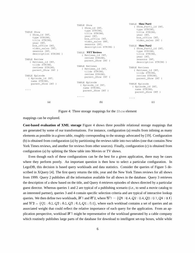
TABLE Show( Show_id INT,

type STRING,title STRING,year INT,box_office INT,video_sales INT,seasons INT,description STRING )

TABLE Review( Reviews_id INT,

tilde STRING,reviews STRING,parent_Show INT )

TABLE Episode( Episode_id INT,name STRING,parent_Show INT )

....

TABLE Show( Show_id INT,

type STRING,title STRING,year INT,box_office INT,video_sales INT,seasons INT,description STRING )

TABLE NYT˙Reviews( Reviews_id INT,

review STRING,parent_Show INT )

TABLE Reviews( Reviews_id INT,

tilde STRING,review STRING,parent_Show INT )

TABLE Episode( Episode_id INT,

name STRING,parent_Show INT )

.....

TABLE Show˙Part1( Show_Part1_id INT,type STRING,title STRING,year INT,box_office INT,video_sales INT )

TABLE Show˙Part2( Show_Part2_id INT,type STRING,title STRING,year INT,seasons INT,description STRING )

TABLE Reviews( Reviews_id INT,tilde STRING,review STRING,parent_Show INT )

TABLE Episode( Episode_id INT,name STRING,parent_Show INT )

....

(a) (b) (c)

Figure 4: Three storage mappings for the Show element

mappings can be explored.

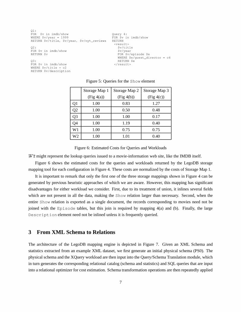
Cost-based evaluation of XML storage Figure 4 shows three possible relational storage mappings that

are generated by some of our transformations. For instance, configuration (a) results from inlining as many

elements as possible in a given table, roughly corresponding to the strategy advocated by [19]. Configuration

(b) is obtained from configuration (a) by partitioning the reviews table into two tables (one that contains New

York Times reviews, and another for reviews from other sources). Finally, configuration (c) is obtained from

configuration (a) by splitting the Show table into Movies or TV shows.

Even though each of these configurations can be the best for a given application, there may be cases

where they perform poorly. An important question is then how to select a particular configuration. In

LegoDB, this decision is based query workloads and data statistics. Consider the queries of Figure 5 de-

scribed in XQuery [4]. The first query returns the title, year and the New York Times reviews for all shows

from 1999. Query 2 publishes all the information available for all shows in the database. Query 3 retrieves

the description of a show based on the title, and Query 4 retrieves episodes of shows directed by a particular

guest director. Whereas queries 1 and 2 are typical of a publishing scenario (i.e., to send a movie catalog to

an interested partner), queries 3 and 4 contain specific selection criteria and are typical of interactive lookup

queries. We then define two workloads,���

and���

, where����� �� �� ������� � �� ������� ��� �������� � �� ����� �

and����� �� ���������� � ���������� ��� �������� � �������� � , where each workload contains a set of queries and an

associated weight that could reflect the relative importance of each query for the application. From an ap-

plication perspective, workload���

might be representative of the workload generated by a cable company

which routinely publishes large parts of the database for download to intelligent set-top boxes, while while

6

Q1:FOR $v in imdb/showWHERE $v/year = 1999RETURN $v/title, $v/year, $v/nyt_reviews

Q2:FOR $v in imdb/showRETURN $v

Q3:FOR $v in imdb/showWHERE $v/title = c2RETURN $v/description

Query 4:FOR $v in imdb/showRETURN<result>

$v/title$v/yearFOR $v/episode $eWHERE $e/guest_director = c4RETURN $e

</result>

Figure 5: Queries for the Show element

Storage Map 1 Storage Map 2 Storage Map 3

(Fig 4(a)) (Fig 4(b)) (Fig 4(c))

Q1 1.00 0.83 1.27

Q2 1.00 0.50 0.48

Q3 1.00 1.00 0.17

Q4 1.00 1.19 0.40

W1 1.00 0.75 0.75

W2 1.00 1.01 0.40

Figure 6: Estimated Costs for Queries and Workloads���

might represent the lookup queries issued to a movie-information web site, like the IMDB itself.

Figure 6 shows the estimated costs for the queries and workloads returned by the LegoDB storage

mapping tool for each configuration in Figure 4. These costs are normalized by the costs of Storage Map 1.

It is important to remark that only the first one of the three storage mappings shown in Figure 4 can be

generated by previous heuristic approaches of which we are aware. However, this mapping has significant

disadvantages for either workload we consider. First, due to its treatment of union, it inlines several fields

which are not present in all the data, making the Show relation larger than necessary. Second, when the

entire Show relation is exported as a single document, the records corresponding to movies need not be

joined with the Episode tables, but this join is required by mapping 4(a) and (b). Finally, the large

Description element need not be inlined unless it is frequently queried.

3 From XML Schema to Relations

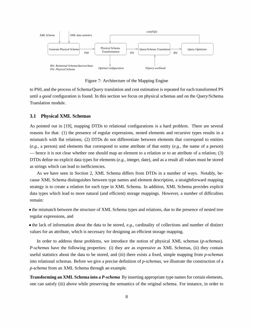
The architecture of the LegoDB mapping engine is depicted in Figure 7. Given an XML Schema and

statistics extracted from an example XML dataset, we first generate an initial physical schema (PS0). The

physical schema and the XQuery workload are then input into the Query/Schema Translation module, which

in turn generates the corresponding relational catalog (schema and statistics) and SQL queries that are input

into a relational optimizer for cost estimation. Schema transformation operations are then repeatedly applied

7

Generate Physical Schema Physical SchemaTransformation

Query/Schema Translation Query Optimizer

XML Schema XML data statistics

Optimal configuration

cost(SQi)

PS0

XQuery workload

RSiPSi

RSi: Relational Schema/Queries/StatsPSi: Physical Schema

Figure 7: Architecture of the Mapping Engine

to PS0, and the process of Schema/Query translation and cost estimation is repeated for each transformed PS

until a good configuration is found. In this section we focus on physical schemas and on the Query/Schema

Translation module.

3.1 Physical XML Schemas

As pointed out in [19], mapping DTDs to relational configurations is a hard problem. There are several

reasons for that: (1) the presence of regular expressions, nested elements and recursive types results in a

mismatch with flat relations; (2) DTDs do not differentiate between elements that correspond to entities

(e.g., a person) and elements that correspond to some attribute of that entity (e.g., the name of a person)

— hence it is not clear whether one should map an element to a relation or to an attribute of a relation; (3)

DTDs define no explicit data types for elements (e.g., integer, date), and as a result all values must be stored

as strings which can lead to inefficiencies.

As we have seen in Section 2, XML Schema differs from DTDs in a number of ways. Notably, be-

cause XML Schema distinguishes between type names and element description, a straightforward mapping

strategy is to create a relation for each type in XML Schema. In addition, XML Schema provides explicit

data types which lead to more natural (and efficient) storage mappings. However, a number of difficulties

remain:

� the mismatch between the structure of XML Schema types and relations, due to the presence of nested tree

regular expressions, and

� the lack of information about the data to be stored, e.g., cardinality of collections and number of distinct

values for an attribute, which is necessary for designing an efficient storage mapping.

In order to address these problems, we introduce the notion of physical XML schemas (p-schemas).

P-schemas have the following properties: (i) they are as expressive as XML Schemas, (ii) they contain

useful statistics about the data to be stored, and (iii) there exists a fixed, simple mapping from p-schemas

into relational schemas. Before we give a precise definition of p-schemas, we illustrate the construction of a

p-schema from an XML Schema through an example.

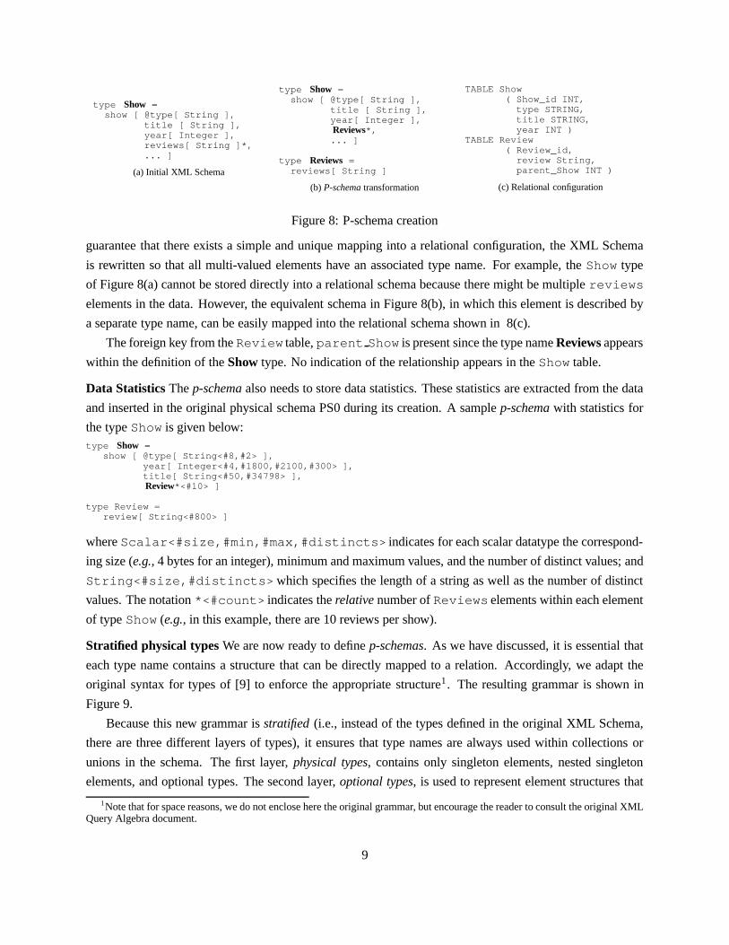
Transforming an XML Schema into a P-schema By inserting appropriate type names for certain elements,

one can satisfy (iii) above while preserving the semantics of the original schema. For instance, in order to

8

type Show =show [ @type[ String ],

title [ String ],year[ Integer ],reviews[ String ]*,... ]

(a) Initial XML Schema

type Show =show [ @type[ String ],

title [ String ],year[ Integer ],Reviews*,... ]

type Reviews =reviews[ String ]

(b) P-schema transformation

TABLE Show( Show_id INT,type STRING,title STRING,year INT )

TABLE Review( Review_id,review String,parent_Show INT )

(c) Relational configuration

Figure 8: P-schema creation

guarantee that there exists a simple and unique mapping into a relational configuration, the XML Schema

is rewritten so that all multi-valued elements have an associated type name. For example, the Show type

of Figure 8(a) cannot be stored directly into a relational schema because there might be multiple reviews

elements in the data. However, the equivalent schema in Figure 8(b), in which this element is described by

a separate type name, can be easily mapped into the relational schema shown in 8(c).

The foreign key from the Review table, parent Show is present since the type name Reviews appears

within the definition of the Show type. No indication of the relationship appears in the Show table.

Data Statistics The p-schema also needs to store data statistics. These statistics are extracted from the data

and inserted in the original physical schema PS0 during its creation. A sample p-schema with statistics for

the type Show is given below:type Show =

show [ @type[ String<#8,#2> ],year[ Integer<#4,#1800,#2100,#300> ],title[ String<#50,#34798> ],Review*<#10> ]

type Review =review[ String<#800> ]

where Scalar<#size,#min,#max,#distincts> indicates for each scalar datatype the correspond-

ing size (e.g., 4 bytes for an integer), minimum and maximum values, and the number of distinct values; and

String<#size,#distincts>which specifies the length of a string as well as the number of distinct

values. The notation *<#count> indicates the relative number of Reviews elements within each element

of type Show (e.g., in this example, there are 10 reviews per show).

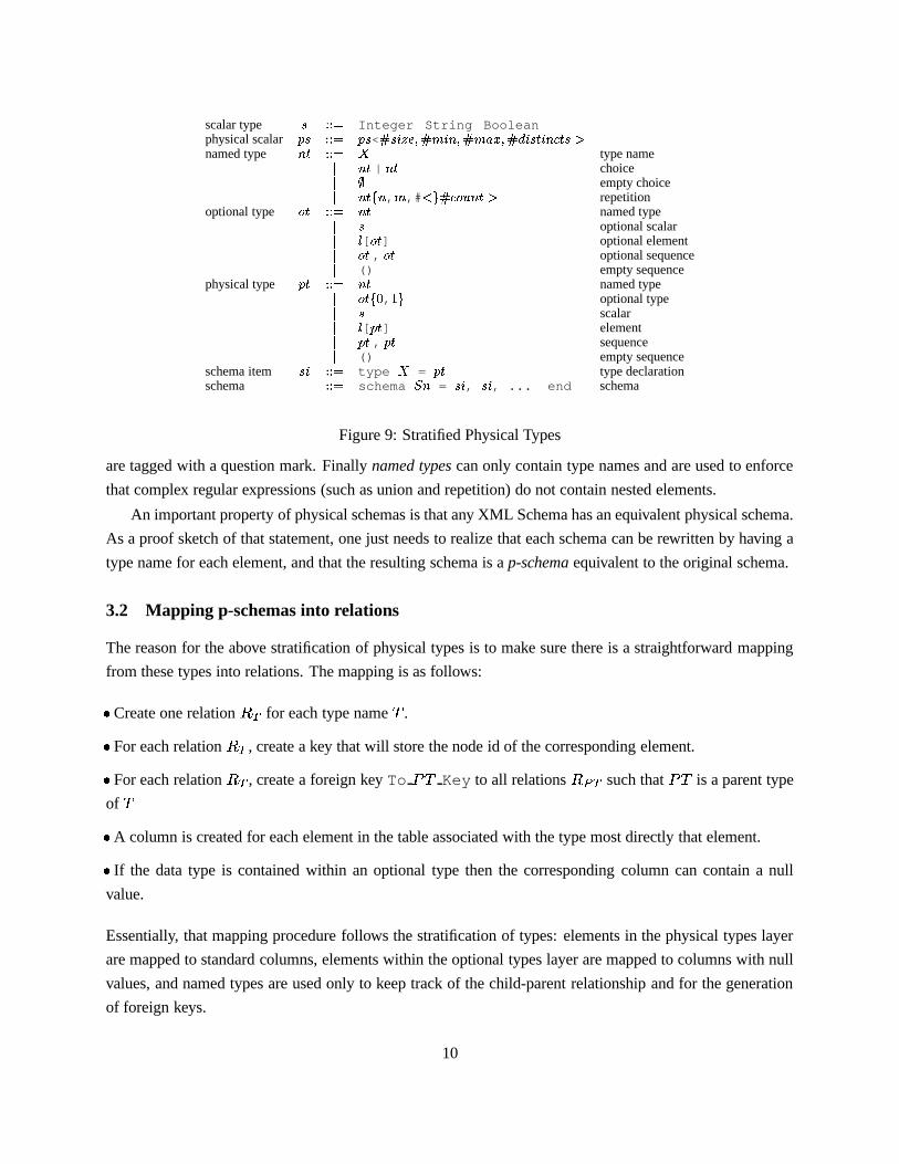
Stratified physical types We are now ready to define p-schemas. As we have discussed, it is essential that

each type name contains a structure that can be directly mapped to a relation. Accordingly, we adapt the

original syntax for types of [9] to enforce the appropriate structure1 . The resulting grammar is shown in

Figure 9.

Because this new grammar is stratified (i.e., instead of the types defined in the original XML Schema,

there are three different layers of types), it ensures that type names are always used within collections or

unions in the schema. The first layer, physical types, contains only singleton elements, nested singleton

elements, and optional types. The second layer, optional types, is used to represent element structures that

1Note that for space reasons, we do not enclose here the original grammar, but encourage the reader to consult the original XMLQuery Algebra document.

9

scalar type � ��� � Integer�String

�Boolean

physical scalar � ����� � � � < � ���� �� ��� ���� ������� � ��� ��������� �!�#"named type ���$��� � % type name� �&� | �&� choice� '

empty choice� �&�)(*� , � ,# +-,.� ��/102�&�3" repetitionoptional type /4�5��� � ��� named type� � optional scalar� 6

[ /4� ] optional element� /4� , /4� optional sequence�() empty sequence

physical type � �7��� � �&� named type� /4�)(18 , 91, optional type� � scalar� 6[� � ] element� � � , � � sequence�() empty sequence

schema item �*7��� � type % = � � type declarationschema ��� � schema : � = �* , � , ... end schema

Figure 9: Stratified Physical Types

are tagged with a question mark. Finally named types can only contain type names and are used to enforce

that complex regular expressions (such as union and repetition) do not contain nested elements.

An important property of physical schemas is that any XML Schema has an equivalent physical schema.

As a proof sketch of that statement, one just needs to realize that each schema can be rewritten by having a

type name for each element, and that the resulting schema is a p-schema equivalent to the original schema.

3.2 Mapping p-schemas into relations

The reason for the above stratification of physical types is to make sure there is a straightforward mapping

from these types into relations. The mapping is as follows:

� Create one relation ;=< for each type name > .

� For each relation ;�< , create a key that will store the node id of the corresponding element.

� For each relation ;=< , create a foreign key To ?@> Key to all relations ;BAC< such that ?@> is a parent type

of >� A column is created for each element in the table associated with the type most directly that element.

� If the data type is contained within an optional type then the corresponding column can contain a null

value.

Essentially, that mapping procedure follows the stratification of types: elements in the physical types layer

are mapped to standard columns, elements within the optional types layer are mapped to columns with null

values, and named types are used only to keep track of the child-parent relationship and for the generation

of foreign keys.

10

For an instance ��� of the p-schema, the relational schema defined by the above mapping is referred to as����������� . Table 1 describe these mappings in detail (except computation of foreign keys). For instance: fixed

size strings in XML are mapped to fixed sized strings in relational; nested elements are mapped to columns;

top level types that contain data types are mapped to a special column that contains a data column, etc.

The function is used to map nested elements, the �� function is used to map optional nested elements and

the ����������� function computes the appropriate foreign key for each table. In fact, a similar function is used

to propagate statistics from the p-schema to the relational schema, but this process is straightforward and

omitted for clarity.

P-schema Relational SchemaDatatypes� � String #<size> ��� ��� � CHAR(size)� � String ��� ��� � STRING� � Integer#<size>

��� ��� � INTEGER

������ � String #<size> ����� ��� � CHAR(size) null� � String ����� ��� � STRING null� � Integer#<size>

� ��� ��� � INTEGER null

�����Elements� � a[ �"! ] ��� ��� �$# a:a1: � � � ���%� a:an:� �'&)( , where ��� �"!*� �$# a1: � �,+� ����� an: � �&)(� �.-[ �/! ] ��� ��� �0# tilde STRING a:a1: � ��� ����� a:an:� �'&)( , where ��� �/!1� �0# a1: � �,+� �%���

an: � � & (� � � 9 , ��2 ��� ��� �$# a1: � � � ����� an:� � & , a1’: � � � ����� am’:� � & ( ,where ��� � 9 � �$# a1: � � + � ���� an: � � & ( and ��� ��2,� �3# a1’: � � + � ���� am’: � � & (� � /1� (18 , 91, ��� /1��� � � ��� /4����&� ��� �&��� �3#4(

Schematype T �String<#count>

TABLE T # T id INT � � � � � CHAR(size) ( 56# �2��7 *�&� �18 ��(

type T � Integer TABLE T # T id INT � � � � � INT ( 56# �2��7 4�&� �18 ��(�����type T = pt TABLE T # T id INT (�5 ��� � ����56# �2��7 *��� �18 ��(

Table 1: Mapping from Physical XML Schemas to Relations

It is noteworthy to mention that, although simple, this mapping deals appropriately with recursive types.

In addition, it also maps XML Schema wildcards (the�

elements) appropriately. Take for example the

definition of the AnyElement in the XML Query Algebra:type AnyElement = ˜[ (AnyElement|AnyScalar)* ]type AnyScalar = Integer | String

This type is valid for all possible elements with any content. In other words, this is a type for untyped XML

documents. Note also that this definition uses both recursive types (AnyElement is used in the content

of any elements) and a wildcard (�

). Again, applying the above rules, one would construct the following

relational schema:TABLE String TABLE Int TABLE AnyElement =( __data STRING, ( __data INT, ( Element_id ID,parent INT ) parent INT ) tilde STRING,

parent_Element INT )

11

This also shows that using XML Schema and the proposed mapping, LegoDB can deal with structured

and semistructured documents in an homogeneous way. Indeed the AnyElement table is similar to the

overflow relation that was used to deal with semistructured document in the STORED system [7].

3.3 Mapping XQuery queries

Although query mapping is an important part of the optimization process, rewriting XML queries into their

equivalent SQL counterparts is not the focus of this paper and we omit any further discussion on this issue.

We refer the interested reader to recently proposed mapping algorithms from XML query languages to

SQL [10, 3].

4 Schema Transformations and Search

In this section, we describe possible transformations for p-schemas. By repeatedly applying these transfor-

mations, LegoDB generates a space of alternative p-schemas and corresponding relational configurations.

As this space can be rather large (possibly infinite), we use a greedy search algorithm that our experiments

show to be effective in practice (see Section 5). The greedy search algorithm and its interaction with a

relational optimizer are presented below in Section 4.2.

4.1 XML transformations

Before we define the p-schema transformations, it is worth pointing out that there are important benefits to

performing these transformations at the XML Schema level as opposed to transforming relational schemas.

Much of the semantics available in the XML schema is not present in a given relational schema and per-

forming the equivalent rewriting at the relational level would imply complex integrity constraints that are not

within the scope of relational keys and foreign keys. As an example, consider the rewriting on Figure 4(c):

such partitioning of the Show table would be very hard to come up with just considering the original schema

(a). On the other hand, we will see that this is a natural rewriting to perform at the XML level. In addi-

tion, working at the XML Schema level makes the framework more easily extensible to other non-relational

stores such as native XML stores and flat files, where a search space based on relational schemas would be

an obstacle.

There are indeed a very large number of possible rewritings applicable to XML Schemas. Instead of

trying to give an exhaustive set of rewriting, we focus on a limited set of such rewritings that correspond to

interesting storage alternatives, and that our experiments show to be beneficial in practice.

Inlining/Outlining As we pointed out several times, one can either associate a type name to a given nested

element (outlining) or nest its definition directly within its parent element (inlining). Rewriting a XML

schema in that way impacts the relational schema by inlining or outlining the corresponding element within

it’s parent table. Inlining is illustrated below using the TV type of Figure 2(b).

12

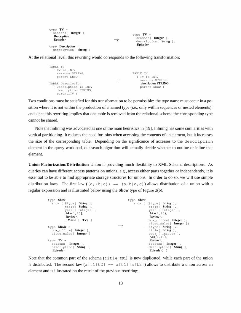
type TV =seasons[ Integer ],Description,Episode*

type Description =description[ String ]

���

type TV =seasons[ Integer ],description[ String ],Episode*

At the relational level, this rewriting would corresponds to the following transformation:

TABLE TV( TV_id INT,

seasons STRING,parent_Show )

TABLE Description( Description_id INT,

description STRING,parent_TV )

���

TABLE TV( TV_id INT,

seasons STRING,description STRING,parent_Show )

Two conditions must be satisfied for this transformation to be permissible: the type name must occur in a po-

sition where it is not within the production of a named type (i.e., only within sequences or nested elements);

and since this rewriting implies that one table is removed from the relational schema the corresponding type

cannot be shared.

Note that inlining was advocated as one of the main heuristics in [19]. Inlining has some similarities with

vertical partitioning. It reduces the need for joins when accessing the contents of an element, but it increases

the size of the corresponding table. Depending on the significance of accesses to the description

element in the query workload, our search algorithm will actually decide whether to outline or inline that

element.

Union Factorization/Distribution Union is providing much flexibility to XML Schema descriptions. As

queries can have different access patterns on unions, e.g., access either parts together or independently, it is

essential to be able to find appropriate storage structures for unions. In order to do so, we will use simple

distribution laws. The first law ((a,(b|c)) == (a,b|a,c)) allows distribution of a union with a

regular expression and is illustrated below using the Show type of Figure 2(b).

type Show =show [ @type[ String ],

title[ String ],year [ Integer ],Aka

�1,10 � ,

Review*,( Movie | TV) ]

type Movie =box_office[ Integer ],video_sales[ Integer ]

type TV =seasons[ Integer ],description[ String ],Episode*

���

type Show =show [ (@type[ String ],

title[ String ],year [ Integer ],Aka

�1,10 � ,

Review*,box_office[ Integer ],video_sales[ Integer ])

| (@type[ String ],title[ String ],year [ Integer ],Aka

�1,10 � ,

Review*,seasons[ Integer ],description[ String ],Episode*) ]

Note that the common part of the schema (title, etc.) is now duplicated, while each part of the union

is distributed. The second law (a[t1|t2] == a[t1]|a[t2]) allows to distribute a union across an

element and is illustrated on the result of the previous rewriting:

13

type Show =show [ (@type[ String ],

title[ String ],year [ Integer ],Aka

�1,10 � ,

Review*,box_office[ Integer ],video_sales[ Integer ])

| (@type[ String ],title[ String ],year [ Integer ],Aka

�1,10 � ,

Review*,seasons[ Integer ],description[ String ],Episode*) ]

���

type Show =( Show˙Part1 | Show˙Part2)

type Show˙Part1 =show [ @type[ String ],

title[ String ],year [ Integer ],Aka

�1,10 � ,

Review*,box_office[ Integer ],video_sales[ Integer ] ]

type Show˙Part2 =show [ @type[ String ],

title[ String ],year [ Integer ],Aka

�1,10 � ,

Review*,seasons[ Integer ],description[ String ],Episode* ]

Here the distribution is done across element boundaries. This sequence of rewriting corresponds to the

following relational configurations:TABLE Show( Show_id INT,

type STRING,title STRING,year INT )

TABLE Movie( Movie_id INT,

box_office INT,video_sales INT,parent_Show INT )

TABLE TV( TV_id INT,

seasons INT,description STRING,parent_Show INT )

���

TABLE Show_Part1( Show_Part1_id INT,

type STRING,title STRING,year INT,box_office INT,video_sales INT )

TABLE Show_Part2( Show_Part2_id INT,

type STRING,title STRING,year INT,seasons INT,description STRING )

This results in the schema given on Figure 4(c) in Section 2. There are a few important remarks to be made

here. First, this rewriting is similar to some form of horizontal partitioning, as Shows with different content

will be split in different tables. Still, that partitioning follows the structure of the XML Schema which

might correspond to quite complex criteria on the original relational schema. Note that the intermediate

step in this rewriting is not a valid p-schema and will not be evaluated for cost before the second half of the

transformation is applied. To the best of our knowledge, no previous XML storage approach has considered

a similar rewriting.

Repetition Merge/Split Another useful rewriting exploits the relationship between sequencing and repeti-

tion in regular expressions by turning one into the other. The corresponding law over regular expressions

(a+ == a,a*) is illustrated below on the aka element in the Show type of Figure 2(b).

type Show =show [ @type[ String ],

title [ String ],year[ Integer ],Aka

�1,* � ]

���

type Show =show [ @type[ String ],

title [ String ],year[ Integer ],Aka, Aka

�0,* � ]

���

type Show =show [ @type[ String ],

title [ String ],year[ Integer ],aka [ String ],Aka

�0,* � ]

Followed by the appropriate inlining, this transformation captures the following relational configurations:

14

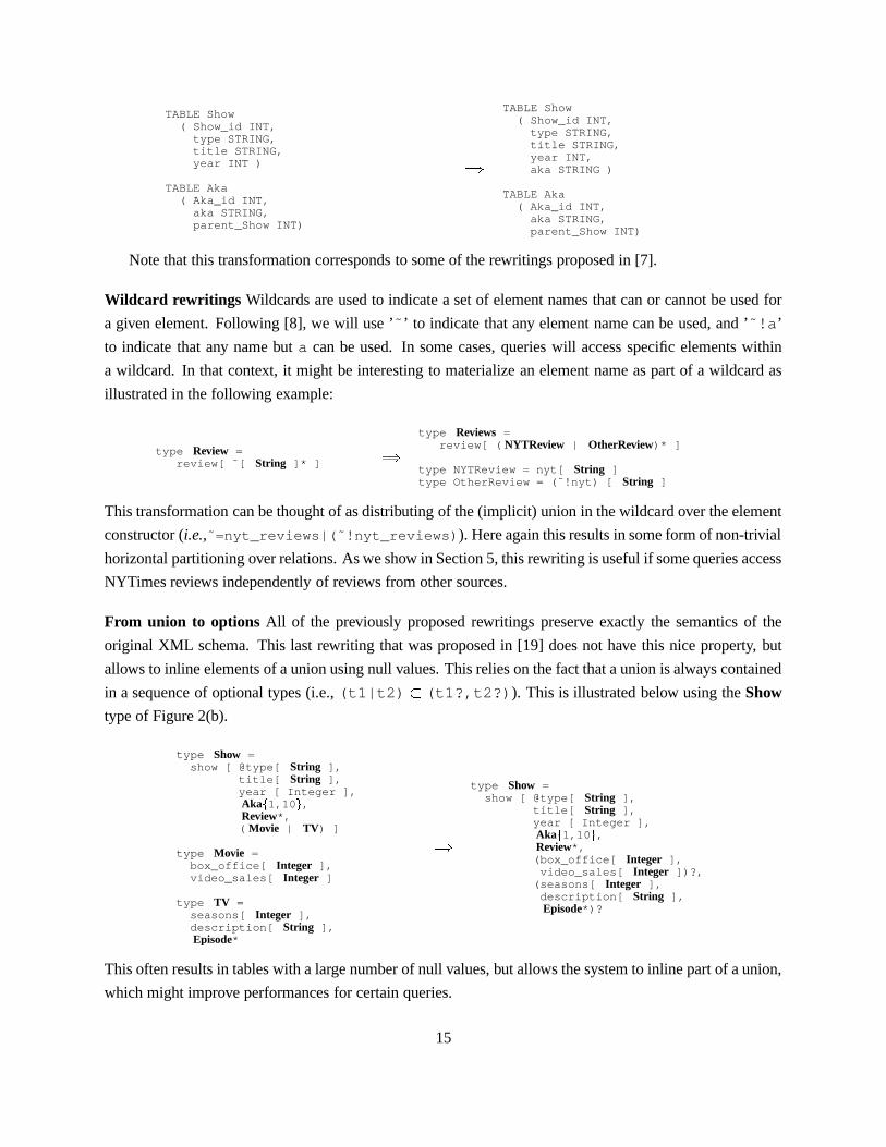
TABLE Show( Show_id INT,

type STRING,title STRING,year INT )

TABLE Aka( Aka_id INT,

aka STRING,parent_Show INT)

���

TABLE Show( Show_id INT,

type STRING,title STRING,year INT,aka STRING )

TABLE Aka( Aka_id INT,

aka STRING,parent_Show INT)

Note that this transformation corresponds to some of the rewritings proposed in [7].

Wildcard rewritings Wildcards are used to indicate a set of element names that can or cannot be used for

a given element. Following [8], we will use ’˜’ to indicate that any element name can be used, and ’˜!a’

to indicate that any name but a can be used. In some cases, queries will access specific elements within

a wildcard. In that context, it might be interesting to materialize an element name as part of a wildcard as

illustrated in the following example:

type Review =review[ ˜[ String ]* ]

���

type Reviews =review[ ( NYTReview | OtherReview)* ]

type NYTReview = nyt[ String ]type OtherReview = (˜!nyt) [ String ]

This transformation can be thought of as distributing of the (implicit) union in the wildcard over the element

constructor (i.e.,˜=nyt_reviews|(˜!nyt_reviews)). Here again this results in some form of non-trivial

horizontal partitioning over relations. As we show in Section 5, this rewriting is useful if some queries access

NYTimes reviews independently of reviews from other sources.

From union to options All of the previously proposed rewritings preserve exactly the semantics of the

original XML schema. This last rewriting that was proposed in [19] does not have this nice property, but

allows to inline elements of a union using null values. This relies on the fact that a union is always contained

in a sequence of optional types (i.e., (t1|t2) �(t1?,t2?)). This is illustrated below using the Show

type of Figure 2(b).

type Show =show [ @type[ String ],

title[ String ],year [ Integer ],Aka

�1,10 � ,

Review*,( Movie | TV) ]

type Movie =box_office[ Integer ],video_sales[ Integer ]

type TV =seasons[ Integer ],description[ String ],Episode*

���

type Show =show [ @type[ String ],

title[ String ],year [ Integer ],Aka

�1,10 � ,

Review*,(box_office[ Integer ],video_sales[ Integer ])?,

(seasons[ Integer ],description[ String ],Episode*)?

This often results in tables with a large number of null values, but allows the system to inline part of a union,

which might improve performances for certain queries.

15

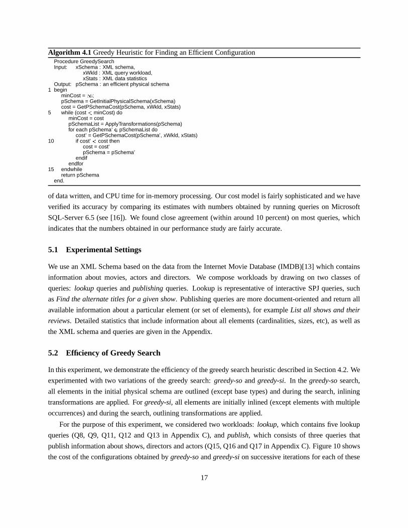
4.2 Search Algorithm

The exploration of the space of storage mappings is described in Algorithm 4.1. Note that the set of config-

urations that result from applying the various schema transformations is very large (possibly infinite), and

since for each configuration queries and statistics must be translated and sent to the optimizer, this process

is likely to take an excessive amount of time to complete and may be infeasible in some cases. Instead of

exhaustively searching the space of all possible configurations, we use a greedy heuristic to find an efficient

configuration.

The algorithm begins by deriving an initial configuration � ����� ��� � from the given XML Schema� ����� ��� � (line 3); details of how this initial configuration is derived appear in Section 3.1. Next, the

cost of this configuration, with respect to the given query workload � � ��� and the data statistics � � ��� �� is

computed using the function ��� ? ����� ��� ����� ��� which will be described in a moment (line 3). The greedy

search (lines 5-16) iteratively updates � ����� ��� � to the cheapest configuration that can be derived from� ����� ��� � using a single transformation. Specifically, in each iteration, a list of candidate configurations� ����� ��� ����� �)� is created by applying all applicable transformations to the current configuration � ����� ��� �(line 7). Each of these candidate configurations is evaluated using ��� ? ����� ��� ����� �)� and the configuration

with the smallest cost is selected (lines 8-14). This process is repeated until the current configuration can no

longer be improved.

We now give details of how ��� ? ����� ��� ����� �)� computes the cost of a given configuration � ����� ��� �given the XML Query workload � �� ��� and the XML data statistics � � �%����� . First, � ����� ��� � is used to

derive the corresponding relation schema (see Section 3.2). This correspondence is also used to translate� � �%����� into the corresponding statistics for the relational data, as well as to translate individual queries in� � ��� into the corresponding relational queries in SQL. The resulting relational schema and the statistics

are used by a relational optimizer to compute the expected cost of computing a query in the SQL workload

derived as above; this cost is returned as the cost of the given � ����� ��� � . Note that the algorithm does not

put any restriction on the kind of optimizer used (transformational or rule-based, linear or bushy, etc. [12]);

though for the exercise to make sense it is expected that it should be same as (or similar to) the optimizer

used in the relational system which is going to be configured based on the recommendations of our mapper.

As we shall see in Section 5, configurations with significantly lower costs can be found through this

greedy search.

5 Performance

The various components of LegoDB (i.e., physical schema creation, schema transformation, and query

translation) have been implemented in a prototype system. Our initial prototype is limited to exploring

inlining/outlining rules in the greedy search—the other XML transformations are explored separately.

To evaluate the alternative configurations in our mapping engine (see Section 3), we used a variation of

the Volcano relational query optimizer [12], as described in [16]. The cost of a query estimated by the query

optimizer on the basis of a cost model that takes into account number of seeks, amount of data read, amount

16

Algorithm 4.1 Greedy Heuristic for Finding an Efficient ConfigurationProcedure GreedySearchInput: xSchema : XML schema,

xWkld : XML query workload,xStats : XML data statistics

Output: pSchema : an efficient physical schema1 begin

minCost = � ;pSchema = GetInitialPhysicalSchema(xSchema)cost = GetPSchemaCost(pSchema, xWkld, xStats)

5 while (cost � minCost) dominCost = costpSchemaList = ApplyTransformations(pSchema)for each pSchema’ � pSchemaList do

cost’ = GetPSchemaCost(pSchema’, xWkld, xStats)10 if cost’ � cost then

cost = cost’pSchema = pSchema’

endifendfor

15 endwhilereturn pSchema

end.

of data written, and CPU time for in-memory processing. Our cost model is fairly sophisticated and we have

verified its accuracy by comparing its estimates with numbers obtained by running queries on Microsoft

SQL-Server 6.5 (see [16]). We found close agreement (within around 10 percent) on most queries, which

indicates that the numbers obtained in our performance study are fairly accurate.

5.1 Experimental Settings

We use an XML Schema based on the data from the Internet Movie Database (IMDB)[13] which contains

information about movies, actors and directors. We compose workloads by drawing on two classes of

queries: lookup queries and publishing queries. Lookup is representative of interactive SPJ queries, such

as Find the alternate titles for a given show. Publishing queries are more document-oriented and return all

available information about a particular element (or set of elements), for example List all shows and their

reviews. Detailed statistics that include information about all elements (cardinalities, sizes, etc), as well as

the XML schema and queries are given in the Appendix.

5.2 Efficiency of Greedy Search

In this experiment, we demonstrate the efficiency of the greedy search heuristic described in Section 4.2. We

experimented with two variations of the greedy search: greedy-so and greedy-si. In the greedy-so search,

all elements in the initial physical schema are outlined (except base types) and during the search, inlining

transformations are applied. For greedy-si, all elements are initially inlined (except elements with multiple

occurrences) and during the search, outlining transformations are applied.

For the purpose of this experiment, we considered two workloads: lookup, which contains five lookup

queries (Q8, Q9, Q11, Q12 and Q13 in Appendix C), and publish, which consists of three queries that

publish information about shows, directors and actors (Q15, Q16 and Q17 in Appendix C). Figure 10 shows

the cost of the configurations obtained by greedy-so and greedy-si on successive iterations for each of these

17

0

20

40

60

80

100

0 50 100 150 200 250 300

cost

iteration

greedy-sigreedy-so

(a) Lookup

0

20

40

60

80

100

0 50 100 150 200 250

cost

iteration

greedy-sigreedy-so

(b) Publish

Figure 10: Cost at each greedy iteration

workloads. Each iteration took approximately 3 seconds.

An interesting observation is that greedy-so converges to the final configuration a lot faster than greedy-

si for lookup queries, while the opposite happens for publish queries, i.e., greedy-si converges faster. This

can be explained as follows. The traversals made by lookup queries are localized. Therefore, the final

configuration has only a few inlined elements. Naturally, greedy-so can reach this configuration earlier than

greedy-si. On the other hand, since the publish queries typically traverse larger number of elements, the final

configuration has several inlined elements. In this case, therefore, greedy-si can reach this configuration

earlier than greedy-so.

Another point worthy of note is that the curves often have a point after which the improvement between

iterations decreases considerably. This suggests that, as an optimization, we could stop the search as soon

as the improvement falls below a certain threshold.

As the graphs show, greedy-so has higher initial costs for both workloads since it leads to a large number

of tables which must be joined to compute the queries. However, note that both strategies converge to similar

costs (the final configurations are also similar). This trend was observed for all variations of schemas, statis-

tics and workloads we experimented with. For simplicity of presentation, greedy-si is the search strategy

used in the experiments below.

5.3 Sensitivity of configurations to varied workloads

An important feature of the LegoDB framework is that the storage is designed taking an application and its

query workload into account. One interesting question is how the resulting configuration performs if the

workload changes. For example, the search interface of IMDB offers users a fixed set of queries. However,

the frequency of these queries may vary over time. For example, in the week before the Academy Awards,

the frequency of queries about movies may increase considerably. Because in many instances it may not

be feasible to re-generate a new configuration and re-load the data, it is important that a chosen storage

configuration leads to acceptable performance even when the frequency of queries varies.

In order to assess the sensitivity of our resulting configurations to changes in workloads, we created a

18

spectrum of workloads that combined the lookup queries and publish queries in Appendix C in the ratio� � � � � , where ��� ��� ��� is the fraction of lookup queries in the particular workload.

Using the same statistics and XML schema, we ran LegoDB for three workloads corresponding to � ��� ��� � �������and

�����, resulting in the three configurations C[0.25], C[0.50] and C[0.75] attuned to the

respective workloads. Next, we gathered these three resulting configurations and evaluated their costs across

the entire workload spectrum; the cost of a configuration is defined as the average cost of processing a query

on that configuration. We did a similar evaluation with the all-inlined configuration, C[ALL-INLINED].

For the sake of comparison, we also plotted a curve OPT giving, for each workload in the spectrum, the cost

of the configuration obtained by LegoDB for that specific workload — this is a tight upper bound on best

possible cost of a configuration at every point in the spectrum. (Note that, in contrast to the other curves,

OPT does not correspond to a fixed schema.) The results are shown in Figure 11.

Before discussing the results, it is important to understand how inlining could affect the cost of a con-

figuration with respect to a query workload. For queries that traverse the schema contiguously and access

all related attributes, inlining helps by precomputing the numerous joins that may be required during the

traversal. On the other hand, inlining could be a bad idea for several other kinds of queries, for example:

(a) the query does limited, localized traversals and/or does not access all the attributes involved, and so does

not benefit from the inlining but nevertheless pays the overhead of scanning wider relations; (b) the query

has highly selective selection predicates — this could render a selection scan on the inlined wider relation

more expensive than evaluation of the query by joining the filtered non-inlined leaner relations, especially in

the presence of appropriate indexes; (c) the query involves join of attributes not structurally adjacent in the

XML Schema (e.g., actor and director) — since inlining causes respective relations to widen due to

the inclusion of several additional attributes not required in the join, the join is significantly more expensive

than in the case of other configurations. These two opposing factors lead to the possibility of different sets

of inlining decisions for different workloads, each optimal in a certain region in the spectrum.

Overlap between the curves for C[0.25] and C[0.75] with the curve for OPT in the graph suggests that

we can partition our spectrum into two regions: the region defined by ��� ��� ������� � and the region defined

by � � ������� � ��� such that C[0.25] is the optimal configuration for all workloads in the former region and

C[0.75] is the optimal configuration for all workloads in the latter (or near enough). Moreover, the curves

for C[0.25] and C[0.75] cross at a small angle. This further implies that even if the two workloads lie in

different regions but are not too distant, the optimal configurations for the two are close enough in cost.

This shows that the configurations found by LegoDB are very robust with respect to the variations in the

workloads.

At the extremes of the spectrum, however, we found a significant difference in performance of the

C[0.25] and C[0.75]. Since these two configurations are based on slightly different inlining decisions, we

see that both publish and lookup queries are sensitive to these decisions, and that inlining is indeed an

important transformation. However, C[ALL-INLINED] that includes all the inlining decisions in the above

configurations (and some more) performed two to five times worse than optimal. This demonstrates that

beyond a point, the overheads due to inlining significantly outweigh any benefits.

19

0.0 0.2 0.4 0.6 0.8 1.0

Fraction of Lookup Queries in Workload

0

20

40

60

80

100

Est

imat

ed A

vera

ge Q

uery

Cos

t (s

econ

ds)

C[All-INLINED]C[0.25]C[0.75]OPT

Figure 11: Sensitivity to variations in the workload

In summary, the above analysis clearly demonstrates that the cost-based approach of LegoDB leads

to configurations that are not only 50% to 80% less costly than the rule-of-the-thumb approach of ALL-

INLINED, but also are very robust with respect to the variations in the workloads.

5.4 Effectiveness of XML transformations

In Section 4 we described some XML-specific transformations that generate relational configurations which

had not been considered in previous XML-to-relational mappings. In what follows, we study the perfor-

mance of some of these transformations.

[Q4.] Display the description, title, year for a show with a given title (only TV shows have description)[Q5.] Display the box office, title, year for a show with a given title (only movies have box office)[Q6.] Display the description, box office, title, year for a show with a given title[Q7.] Display the title and year for shows that have an episode directed by a given guest director[Q13.] Find all people that acted and directed in the same movie as well as alternate titles for the movie[Q16.] Publish all shows[Q19.] Publish all the information about a show given its title

Figure 12: Sample Queries

Q4 Q5 Q6 Q7 Q13 Q16 Q190 2 4 6

Query

0

20

40

60

80

100

Cos

t im

prov

emen

t fo

r U

nion

All InlinedUnion distribution

Figure 13: Cost of union-transformed configuration as a percentage of the cost of an all-inlined configuration

Union Distribution In order to measure the effectiveness of union distribution we compared the costs of

20

Total reviews 10,000 100,000NYT perc. Query 1 Query 2 Query 1 Query 250% 5.42 6.3 48 26.325% 5.42 5.1 48 1512.5% 5.42 4.4 48 9.4

Table 2: Cost for all-inlined vs wildcard-transformed

various queries for the configurations illustrated in Figure 4(a) (all elements inlined) and Figure 4(c) (where

union is distributed over show). The queries considered are shown in Figure 12.2

As Figure 13 shows, the union-transformed configuration has lower costs for all queries. In this exam-

ple, the union distribution is equivalent to vertically partitioning the Show table into a table that contains

information about movies, and a table that contains information about TV shows. Because the new tables

are smaller, queries that refer to elements in only one of those tables will be cheaper (e.g., Q4 accesses

descriptions, Q7 accesses episodes, and Q5 accesses box office).

These results are rather intuitive. A less intuitive finding is that even queries that access elements from

both movies and TV shows (e.g., Q6 that retrieves description and box office) become cheaper

under the union rewriting. Even though the original selection query:����������� � ��������������� ��� ��� ����������� � � ��� � �

must be rewritten as the union of two subqueries for the transformed schema����������� ����� �!��������� � � ��� ���������� ��" � � ��� � �$# ����������� % ��& ��'�' ����� ��� ���������

�� � �(" � �)� �

not only does each subquery operate on tables with fewer tuples, but these tables are also narrower which

reduce the cost of selection. This is also true of Q13, Q16 and Q19.

Repetition Split Another transformation we considered is splitting repetitions. This transformation was

illustrated in Section 4. The effectiveness of such a transformation is highly dependent on the characteristics

of the data and on the query workload. Consider for example two queries: a lookup query that finds all of the

alternate titles (akas) for a given show title; and its publishing counterpart which retrieves all information

for all shows. The costs for these two queries under the All Inlined and the Repetition-Split transformed

configurations for a varied number of total akas are given in Figure 14. For this example, the main effect of

the Repetition Split transformation is that it reduces the size of the Aka table. As a result, the cost reduction

is bigger for the publishing query—since the lookup query involves a selection on title and this selection

can be pushed, the size of the Aka table will impact the show-aka join to a lesser extent than in the

publishing query where no selection is performed. Also note that as the size of the Aka table increases (and

becomes much larger than the Show table), the cost difference between the two configurations decrease.

Wildcards The wildcard transformation effectively partitions the set of elements tagged by the wildcard

into different sorts that correspond to the wildcard labels that are present in the data. Consider for example

the query Find the reviews for all shows produced in 1999. The equivalent queries under the configurations

in Figure 4(a) and (b) are:

2The corresponding XQueries are given in Appendix C.

21

4

5

6

7

8

9

10

11

20 40 60 80 100 120 140 160 180 200

cost

total number of akas (*1000)

All inlinedRepetition Split

(a) Lookup

5

10

15

20

25

30

35

40

20 40 60 80 100 120 140 160 180 200

cost

total number of akas (*1000)

All inlinedRepetition Split

(b) Publish

Figure 14: Cost comparison between an all-inlined and a repetition-split configuration

1����������� �

���

���������������� � � ��� ��� ����" �%��� � �

2����������� �

���

���������������� � � ��� ��� ����� ��� " � � � � �

Table 2 shows the cost of these two queries for varying percentage of NYTimes reviews, when the total

number of reviews is 10,000 and 100,000. As expected, whereas the cost for Query 1 remains constant, the

cost for Query 2 decreases with the size of the nyt reviews table.

6 Related Work

In this section we first compare LegoDB to prior work on storing XML data with relational engines. Fol-

lowing this discussion, we outline other related work, in particular the relationship between automatic XML

storage mapping and automatic physical design for relational databases.

Recently, many approaches have been suggested for mapping XML documents to relations for stor-

age [7, 11, 14, 18, 19, 20]. In [7], Deutsch, Fernandez and Suciu propose the STORED system for map-

ping between (schemaless) semi-structured data and the relational data model. They focus on a data mining

technique which simultaneously solves schema discovery and storage mapping by identifying “highly sup-

ported” tree patterns for storage in relations. Even though they considered a cost optimization approach to

the problem, they found it to be impractical, as in the absence of a schema, optimization is shown to be ex-

ponential in the size of the data. In contrast, we explore a space of storage structures but rely on the schema

and statistics rather than directly mining the data. We use heuristics (e.g., the greedy approach) to avoid an

exponential search, but still explore a variety of useful mappings. In fact, the LegoDB strategy may lead to

substantially different configurations than what is produced by the data-mining approach used by STORED.

For example, we may break an extremely common pattern of data into multiple relations if the result is more

efficient for the query workload.

In [19], Shanmugasundaram et al propose three strategies to map DTDs into relational schemas. The

22

basic idea behind these mappings is to create tables that correspond to XML elements defined in a DTD, in-

lining as many sub-elements as possible so as to reduce fragmentation—multi-valued elements and elements

involved in recursive associations must be kept in separate tables. The three proposed mappings differ from

one another in the degree of redundancy: they vary from being highly redundant (where an element can be

stored in multiple tables), to containing no redundancy. While we do not consider mappings which dupli-

cate data, we share with [19] the use of the schema to derive a heuristically “good” initial storage mapping

(e.g., for the greedy-si search strategy), and the use of a modified schema for the storage mapping language.

Regardless of the particular strategy, the mapping process of [19] begins by simplifying an input DTD into

a DTD that can be easily mapped into relations. Instead of simplifying away hard-to-map XML Schema

constructs, LegoDB takes advantage of them (through the use of our schema transformations) to generate

a space of mappings. And as we have shown in Section 5, mappings that result from the XML-specific

transformations may lead to significantly better configurations for a given application than mappings based

on an inline-as-much-as-possible approach.

Schmidt et al [18] propose a highly fragmented relational storage model. In their proposed “Monet

transformation”, the parent-child association terminating each label-path from the root of an XML docu-

ment is stored as a binary relation of oids. Like STORED, they do not require a schema—the document

structure is explored at parsing time. However, unlike Stored, they use a purely relational storage. Their

experiments show that this approach performs well on the main-memory-oriented Monet database, a result

in stark contrast to the conclusions presented in [19] where fragmentation and a large number of joins is

identified as a key problem. These disparate performance results only emphasize the need for automated

tools, like LegoDB, to determine the appropriate storage mapping for a given application and DBMS plat-

form. Finally, while the search space in our work does not include horizontal fragmentation of tables based

on incoming paths, our rewriting rules can easily be extended to consider this style of transformation.

Tian et al [22] compare the performance of several approaches to XML storage, one of which is a rela-

tional mapping similar to our “max-inlined” approach. It would be interesting to see how a more optimized

mapping would affect the performance of the relational mapping relative to their other native and text-based

storage methods. Florescu and Kossman [11] investigated several alternatives when designing a relational

schema for storing an XML document including storing a node table and an edge table, and storing a “uni-

versal relation” with an attribute for every element or attribute name in the document. Shimura et al [20]

propose an inverted-list-style storage structure in which nodes are mapped to regions in the document, and

paths are present as strings in a “Path” table. Path queries are accomplished by using string operators (in

particular the LIKE operator of SQL) to query this table. In all three of these cases, one or more fixed map-

pings are used, where we explore a space of storage mappings. Mappings from DTDs into nested schema

structures of OO or OR/DBMS have been proposed [6, 14]. While Klettke and Meyer consider statistics

and queries in the proposed heuristic mapping, no attempt is made to compare estimated costs for multiple

mappings.

Several commercial DBMSs already offer some support for storing, querying, and exporting XML doc-

uments [24, 15]; however, the user must still design an appropriate storage mapping.

23

While LegoDB is (to our knowledge) the first XML storage mapping tool to take advantage of cost-based

optimization, similar approaches have been applied to problems in relational storage design, such as index

selection (e.g., [17]) and view materialization (e.g., [1, 23]) in physical optimization for relational DBMSs.

Note that physical design tools are complementary to LegoDB, and can be applied to further optimize the

relational schemas produced by our mapping, either during the search process or simply on the final schema

produced.

7 Conclusions

We have introduced LegoDB, a system for generating relational storage mappings for XML data based on

the schema for the data and statistics. In contrast to previous work, we explore a space of alternate storage

configurations and evaluate the quality of each configuration by estimating its performance on an applica-

tion workload. We also make original use of XML Schema to support new possible storage configuration,

and proposed XML Schema rewritings as a means to explore possible configurations. The LegoDB systems

isolate the application developer from the underlying storage engine by taking only XML Schemas, queries

and documents as input. Further, we have presented an initial performance study using a prototype imple-

mentation of our approach in the LegoDB system being built at Bell Labs. This study evaluates a greedy

algorithm to inlining or outlining of elements and attributes. The results indicate that storage mappings of

significantly improved quality can be found in a reasonable number of steps using greedy evaluation, and

that these designs are not overly sensitive to small changes in the workload. In addition, we have shown that

XML transformations other than inlining/outlining can lead to significant performance gains.

We consider this work as a first step towards a general purpose storage configuration engine for XML.

To achieve that goal, we need to extend the LegoDB system in a number of ways. First we plan to adapt our

approach to other storage platforms, such as native stores, text stores, and hybrid storage systems. We plan

to extend the subset of XQuery supported currently by LegoDB, possibly using techniques similar to [3, 10].

Our work can also be extended in several simple ways, such as including updates in our workload, allowing

redundancy in data storage, considering dynamic programming search strategies, etc. Finally, we plan to

decrease the cost of evaluating a particular point in the space by allowing our query optimizer to reuse

partial results from one evaluation to the next, and consider the integration of complementary relational

storage design tools such as [17, 1].

References

[1] S. Agrawal, S. Chaudhuri, and V.R. Narasayya. Automated selection of materialized views and indexes in SQLdatabases. In Proceedings of VLDB, pages 496–505, 2000.

[2] J. Bosac, T. Bray, D. Connolly, E. Maler, G. Nicol, C.M. Sperberg-McQueen, L. Wood, and J. Clark. Guide tothe W3C XML specification (”XMLspec”) DTD. http://www.w3.org/XML/1998/06/xmlspec-report, June 1998.

[3] M.J. Carey, J. Kiernan, J. Shanmugasundaram, E.J. Shekita, and S.N. Subramanian. Xperanto: Middleware forpublishing object-relational data as xml documents. In Proceedings of VLDB, pages 646–648, 2000.

24

[4] D. Chambelin, J. Clark, D. Florescu, Jonathan Robie, J. Simeon, and M. Stefanescu. XQuery 1.0: An XMLquery language. W3C Working Draft, June 2001.

[5] D. Chamberlin, D. Florescu, J. Robie, J. Simeon, and M. Stefanescu. XQuery: A query language for XML,February 2001. W3C Working Draft available at http://www.w3.org/.

[6] V. Christophides, S. Abiteboul, S. Cluet, and M. Scholl. From structured documents to novel query facilities. InProceedings of SIGMOD, pages 313–324, Minneapolis, Minnesota, May 1994.

[7] A. Deutsch, M. Fernandez, and D. Suciu. Storing semi-structured data with STORED. In Proceedings ofSIGMOD, pages 431–442, 1999.

[8] W. Fan, G. Kuper, and J. Simeon. A unified constraint model for XML. In Proceedings of WWW, pages 179–190,Hong Kong, China, May 2001.

[9] P. Fankhauser, M. Fernandez, A. Malhotra, M. Rys, J. Simeon, and P. Wadler. The XML query algebra, February2001. http://www.w3.org/TR/2001/WD-query-algebra-20010215.

[10] M.F. Fernandez, W.C. Tan, and D. Suciu. Silkroute: trading between relations and XML. WWW9/ComputerNetworks, 33(1-6):723–745, 2000.

[11] D. Florescu and D. Kossmann. A performance evaluation of alternative mapping schemes for storing XML in arelational database. Technical Report 3680, INRIA, 1999.

[12] Goetz Graefe and William J. McKenna. The volcano optimizer generator: Extensibility and efficient search. InProceedings of ICDE, 1993.

[13] Internet Movie Database. http://www.imdb.com.

[14] M. Klettke and H. Meyer. XML and object-relational database systems - enhancing structural mappings basedon statistics. In Proceedings of WebDB, pages 63–68, 2000.

[15] M. Rhys. State-of-the-art XML support in RDBMS: Microsoft SQL Server’s XML features. Bulletin of theTechnical Committee on Data Engineering, 24(2):3–11, June 2001.

[16] P. Roy, S. Seshadri, S. Sudarshan, and S. Bhobe. Efficient and extensible algorithms for multi query optimization.In Proceedings of SIGMOD, pages 249–260, 2000.

[17] V.R. Narasayya S. Chaudhuri. Autoadmin ’what-if’ index analysis utility. In Proceedings of SIGMOD, pages367–378, 1998.

[18] A. Schmidt, M. Kersten, M. Windhouwer, and F. Waas. Efficient relational storage and retrieval of XML docu-ments. In Proceedings of WebDB, pages 47–52, 2000.

[19] J. Shanmugasundaram, K. Tufte, G. He, C. Zhang, D. DeWitt, and J. Naughton. Relational databases for queryingXML documents: Limitations and opportunities. In Proceedings of VLDB, pages 302–314, 1999.

[20] T. Shimura, M. Yoshikawa, and S. Uemura. Storage and retrieval of XML documents using object-relationaldatabases. In Proceedings of DEXA, pages 206–217, 1999.

[21] H. Thompson, D. Beech, M. Maloney, and N. Mendelsohn. XML schema part 1: Structures. W3C WorkingDraft, February 2000.

[22] F. Tian, D. DeWitt, J. Chen, and C. Zhung. The design and performance evaluation of various XML storagestrategies. http://www.cs.wisc.edu/niagra/Publications.html, 2001.

[23] O. Tsatalos, M. Solomon, and Y. Ioannidis. The gmap: A versatile tool for physical data independence. InProceedings of VLDB, pages 367–378, 1994.

[24] Oracle’s XML SQL utility. http://technet.oracle.com/tech/xml/oracle xsu.

25

A Statistics(["imdb"], STcnt(1));(["imdb";"director"], STcnt(26251));(["imdb";"director";"name"], STsize(40));(["imdb";"director";"directed"], STcnt(105004));(["imdb";"director";"directed"; "title"], STsize(40));(["imdb";"director";"directed";"year"], STbase(1800,2100,300));(["imdb";"director"; "directed";"info"], STcnt(50000));(["imdb";"director"; "directed";"info"], STsize(100));(["imdb";"director";"directed";"TILDE"], STsize(255));(["imdb";"show"], STcnt(34798));(["imdb";"show";"title"], STsize(50));(["imdb";"show";"year"], STbase(1800,2100,300));(["imdb";"show";"aka"], STcnt(13641));(["imdb";"show";"aka"], STsize(40));(["imdb";"show";"type"], STsize(8));(["imdb";"show";"reviews" ], STcnt(11250));(["imdb";"show";"reviews";"TILDE"], STsize(800));(["imdb";"show";"box_office"], STcnt(7000));(["imdb";"show";"box_office"], STbase(10000,100000000,7000));(["imdb";"show";"video_sales"], STcnt(7000));(["imdb";"show";"video_sales"], STbase(10000,100000000,7000));(["imdb";"show";"seasons"], STcnt(3500));(["imdb";"show";"description"], STsize(120));(["imdb";"show";"episodes"], STcnt(31250));(["imdb";"show";"episodes";"name"], STsize(40));(["imdb";"show";"episodes";"guest_director"], STsize(40));(["imdb";"actor"], STcnt(165786));(["imdb";"actor";"name"], STsize(40));(["imdb";"actor";"played"], STcnt(663144));(["imdb";"actor";"played"; "title"], STsize(40));(["imdb";"actor";"played";"year"], STbase(1800,2100,200));(["imdb";"actor"; "played" ; "character"], STsize(40));(["imdb";"actor";"played";"order_of_appearance"], STbase(1,300,300));(["imdb";"actor"; "played" ; "award";"result"], STsize(3));(["imdb";"actor"; "played" ; "award";"award_name"], STsize(40));(["imdb";"actor"; "biography" ; "birthday"], STsize(10));(["imdb";"actor"; "biography" ; "text"], STcnt(20000));(["imdb";"actor"; "biography" ; "text"], STsize(30))

B Schema

XML Algebra notation

type IMDB =imdb [ Show

�0,* � ,Director �

0,* � ,Actor �0,* � ]

type Show =show [ title [ String ], year[ Integer ], type[ String ],

aka [ String ]�0,* � , reviews[ TILDE[ String ] ]

�0,* � ,

(box_office [ Integer ], video_sales [ Integer ]| seasons[ Integer ], description [ String ],episodes [ name[String], guest_director[ String ]]

�0,* �

)]

type Director =director [ name [String],

directed [ title[ String ], year[ Integer ],info[ String ], TILDE [ String ] ]

�0,* �

]

type Actor =actor [ name [String],

played[ title[ String ], year[ Integer ],character[String], order_of_appearance[Integer],award[ result [String], award_name[String] ]

�0,5 �

]�0,* � ,

biography[ birthday[ String ], text[String] ]

26

]

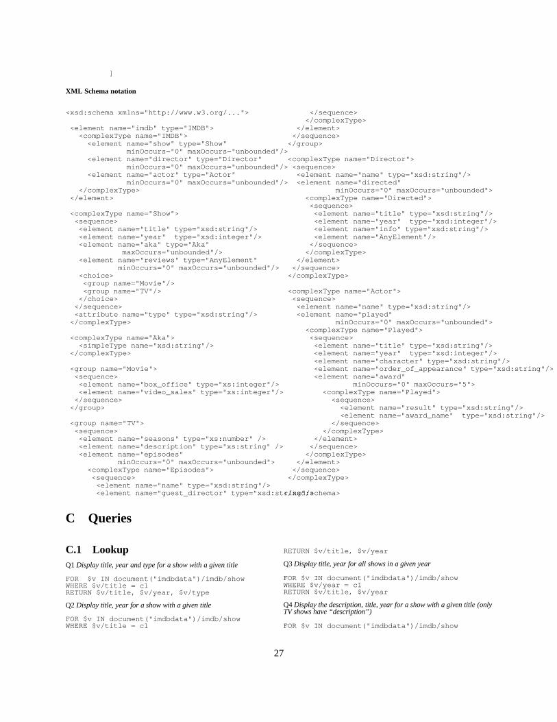
XML Schema notation

<xsd:schema xmlns="http://www.w3.org/...">

<element name="imdb" type="IMDB"><complexType name="IMDB"><element name="show" type="Show"

minOccurs="0" maxOccurs="unbounded"/><element name="director" type="Director"

minOccurs="0" maxOccurs="unbounded"/><element name="actor" type="Actor"

minOccurs="0" maxOccurs="unbounded"/></complexType>

</element>

<complexType name="Show"><sequence><element name="title" type="xsd:string"/><element name="year" type="xsd:integer"/><element name="aka" type="Aka"

maxOccurs="unbounded"/><element name="reviews" type="AnyElement"

minOccurs="0" maxOccurs="unbounded"/><choice><group name="Movie"/><group name="TV"/></choice>

</sequence><attribute name="type" type="xsd:string"/>

</complexType>

<complexType name="Aka"><simpleType name="xsd:string"/>

</complexType>

<group name="Movie"><sequence><element name="box_office" type="xs:integer"/><element name="video_sales" type="xs:integer"/>

</sequence></group>

<group name="TV"><sequence><element name="seasons" type="xs:number" /><element name="description" type="xs:string" /><element name="episodes"

minOccurs="0" maxOccurs="unbounded"><complexType name="Episodes"><sequence><element name="name" type="xsd:string"/><element name="guest_director" type="xsd:string"/>

</sequence></complexType>

</element></sequence></group>

<complexType name="Director"><sequence><element name="name" type="xsd:string"/><element name="directed"

minOccurs="0" maxOccurs="unbounded"><complexType name="Directed"><sequence><element name="title" type="xsd:string"/><element name="year" type="xsd:integer"/><element name="info" type="xsd:string"/><element name="AnyElement"/></sequence></complexType>

</element></sequence></complexType>

<complexType name="Actor"><sequence><element name="name" type="xsd:string"/><element name="played"

minOccurs="0" maxOccurs="unbounded"><complexType name="Played"><sequence><element name="title" type="xsd:string"/><element name="year" type="xsd:integer"/><element name="character" type="xsd:string"/><element name="order_of_appearance" type="xsd:string"/><element name="award"

minOccurs="0" maxOccurs="5"><complexType name="Played">

<sequence><element name="result" type="xsd:string"/><element name="award_name" type="xsd:string"/>

</sequence></complexType>

</element></sequence></complexType>

</element></sequence></complexType>

</xsd:schema>

C Queries

C.1 LookupQ1 Display title, year and type for a show with a given title

FOR $v IN document("imdbdata")/imdb/showWHERE $v/title = c1RETURN $v/title, $v/year, $v/type

Q2 Display title, year for a show with a given title

FOR $v IN document("imdbdata")/imdb/showWHERE $v/title = c1

RETURN $v/title, $v/year

Q3 Display title, year for all shows in a given year

FOR $v IN document("imdbdata")/imdb/showWHERE $v/year = c1RETURN $v/title, $v/year

Q4 Display the description, title, year for a show with a given title (onlyTV shows have “description”)

FOR $v IN document("imdbdata")/imdb/show

27

WHERE $v/title = c1RETURN $v/title, $v/year, $v/description

Q5 Display the box office, title, year for a show with a given title (onlymovies have “box office”)

FOR $v IN document("imdbdata")/imdb/showWHERE $v/title = c1RETURN $v/title, $v/year, $v/box_office

Q6 Display the description, box office, title, year for a show with a giventitle

FOR $v IN document("imdbdata")/imdb/showWHERE $v/title = c1RETURN $v/title, $v/year,

$v/box_office, $v/description

Q7 Display the title and year for shows that have an episode directed bya given guest director

FOR $v IN document("imdbdata")/imdb/showRETURN

$v/title,$v/yearFOR $e IN $v/episodeWHERE $e/guest_director = c1RETURN $e/guest_director

Q8 Display the birthday for an actor given his name

FOR $v IN document("imdbdata")/imdb/actorWHERE $v/name = c1RETURN $v/biography/birthday

Q9 Display the name, biography text for all actors born on a given date

FOR $v IN document("imdbdata")/imdb/actorRETURN<result>$v/nameFOR $v/biography $bwhere $b/birthday = c1RETURN $b/text

</result>

Q10 Display the name, biography text and birthday for all actors bornon a given date

FOR $v IN document("imdbdata")/imdb/actorRETURN<result>$v/nameFOR $v/biography $bwhere $b/birthday = c1RETURN $b

</result>

Q11 Display name and order of appearance for all actors that played agiven character

FOR $v IN document("imdbdata")/imdb/actorRETURN<result>

$v/nameFOR $v/played $pwhere $p/character = c1RETURN $p/order_of_appearance

</result>

Q12 Find all people that acted and directed in the same movie

FOR $i IN document("imdbdata")/imdb$a in $i/actor,$m1 in $a/played,$d in $i/director,$m2 in $a/directed,

WHERE $a/name = $d/name AND $m1/title = $m2/titleRETURN<result>

$a/name$m1/title$m1/year

</result>

Q13 Find all people that acted and directed in the same movie as wellas alternate titles for the movie

FOR $i IN document("imdbdata")/imdb$s in $i/show,$a in $i/actor,$m1 in $a/played,$d in $i/director,$m2 in $a/directed,

WHERE $a/name = $d/name AND$m1/title = $m2/title AND$m1/title = $s/title

RETURN<result>

$a/name$m1/title$m1/yearFOR $v in $s/akaRETURN $v/title

</result>

Q14 Find all directors that directed a given actor

FOR $i IN document("imdbdata")/imdb$a in $i/actor,$m1 in $a/played,$d in $i/director,$m2 in $a/directed,

WHERE $a/name = c1 AND $m1/title = $m2/titleRETURN<result>

$d/name$m1/title$m1/year

</result>

C.2 Publish

Q15 Publish all actors

FOR $a IN document("imdbdata")/imdb/actorRETURN $a

Q16 Publish all shows

FOR $s IN document("imdbdata")/imdb/showRETURN $s

Q17 Publish all directors

FOR $d IN document("imdbdata")/imdb/directorRETURN $d

Q18 Display all info about a given actor

FOR $a IN document("imdbdata")/imdb/actorWHERE $a/name = c1RETURN $a

Q19 Display all info about a given show

FOR $s IN document("imdbdata")/imdb/showWHERE $s/title = c1RETURN $s

Q20 Publish all info about a given director

FOR $d IN document("imdbdata")/imdb/directorWHERE $d/name = c1RETURN $d

28