Front variability and surface ocean features of the presumed southern bluefin tuna spawning grounds in the tropical southeast Indian Ocean

Front variability and surface ocean features of the presumed southernbluefin tuna spawning grounds in the tropical southeast Indian Ocean

Anne-Elise Nieblas a,n,1, Hervé Demarcq b,nn, Kyla Drushka c,2, Bernadette Sloyan a,d,Sylvain Bonhommeau e

a Commonwealth Scientific and Industrial Research Organisation (CSIRO) Wealth from Oceans Research Flagship, GPO Box 1538, Hobart 7001, Australiab Unité Mixte de Recherche Ecosystèmes Marins Exploités 212, Institut de Recherche pour le Développement, Av. J. Monnet, Sète Cedex 34203, Francec Laboratoire d'Océanographie – Expérimentation et Approches Numériques, Case 100 – UPMC 4 place Jussieu, F-75252 Paris, Franced CSIRO Centre for Australian Weather and Climate Research, GPO Box 1538, Hobart 7001, Australiae Unité Mixte de Recherche Ecosystèmes Marins Exploités 212, Institut Français de Recherche pour l’Exploitation de la Mer, Av. J. Monnet,Sète Cedex 34203, France

a r t i c l e i n f o

Keywords:Tropical southeast Indian OceanIndo-Australian regionSouthern bluefin tuna Thunnus maccoyiiSpawning grounds (101S-201S1051E-1251E)Oceanic frontsFront detection index

a b s t r a c t

The southern bluefin tuna (SBT, Thunnus maccoyii) is an ecologically and economically valuable fish.However, surprisingly little is known about its critical early life history, a period when mortality is severalorders of magnitude higher than at any other life stage, and when larvae are highly sensitive toenvironmental conditions. Ocean fronts can be important in creating favourable spawning conditions, asthey are a convergence of water masses with different properties that can concentrate planktonic particlesand lead to enhanced productivity. In this study, we examine the front activity within the only regionwhere SBT have been observed to spawn: the tropical southeast Indian Ocean between Indonesia andAustralia (101S–201S, 1051E–1251E). We investigate front activity and its relationship to ocean dynamicsand surface features of the region. Results are also presented for the entire Indian Ocean (301N–451S,201E–1401E) to provide a background context. We use an extension of the Cayula and Cornillon algorithmto detect ocean fronts from satellite images of sea surface temperature (SST) and chlorophyll-a concen-tration (chl-a). Front occurrence represents the probability of occurrence of a front at each pixel of animage. Front intensity represents the magnitude of the difference between the two water masses thatmake up a front. Relative to the rest of the Indian Ocean, both SST and chl-a fronts in the offshore spawningregion are persistent in occurrence and weak in intensity. Front occurrence and intensity along theAustralian coast are high, with persistent and intense fronts found along the northwest and west coasts.Fronts in the tropical southeast Indian Ocean are shown to have strong annual variability and somemoderate interannual variability. SST front occurrence is found to lead the Southern Oscillation Index byone year, potentially linked to warming and wind anomalies in the Indian Ocean. The surface oceancharacteristics of the offshore SBT spawning region are found to be particularly stable compared to the restof the Indian Ocean in terms of stable SST, low eddy kinetic energy, i.e., low mesoscale eddy activity, andlow chl-a. However, this region has high front occurrence, but low front intensity of both SST and chl-afronts. The potential impact of these oceanic features for SBT spawning is discussed.

& 2013 Elsevier Ltd. All rights reserved.

1. Introduction

The southern bluefin tuna (SBT; Thunnus maccoyii) is aneconomically valuable fish and an ecologically important apex

predator, but despite its importance and a long history of research,knowledge of its early life history is limited. The larval stage isdecisive for the renewal of marine populations as it has thehighest mortality of all life stages (499%; Hjort 1914). Early lifestages are highly sensitive to environmental conditions and fishlarval survival is commonly influenced by retention of larvae inregions where the ocean circulation concentrates food sources(Bakun, 1996). However, the reproductive strategy of bluefin tunais unusual, as they migrate from their temperate and productivefeeding grounds to oligotrophic tropical and subtropical spawninggrounds (Schaefer, 2001; Bakun and Broad, 2003). Bakun andBroad (2003) suggest that the early life stages of tuna are highlyvulnerable to predation, and thus spawning adults seek regions

Contents lists available at ScienceDirect

journal homepage: www.elsevier.com/locate/dsr2

Deep-Sea Research II

0967-0645/$ - see front matter & 2013 Elsevier Ltd. All rights reserved.http://dx.doi.org/10.1016/j.dsr2.2013.11.007

n Corresponding author.nn Corresponding author.E-mail addresses: [email protected] (A.-E. Nieblas),

[email protected] (H. Demarcq).1 Present address: Unité Mixte de Recherche Ecosystèmes Marins Exploités

212, Institut Français de Recherche pour l’Exploitation de la Mer, Av. J. Monnet, SèteCedex 34203, France.

2 Present address: Scripps Institution of Oceanography, La Jolla, CA 92093-0230, USA.

Please cite this article as: Nieblas, A.-E., et al., Front variability and surface ocean features of the presumed southern bluefin tunaspawning grounds in the tropical southeast Indian Ocean. Deep-Sea Res. II (2014), http://dx.doi.org/10.1016/j.dsr2.2013.11.007i

Deep-Sea Research II ∎ (∎∎∎∎) ∎∎∎–∎∎∎

www.sciencedirect.com/science/journal/09670645

www.elsevier.com/locate/dsr2

http://dx.doi.org/10.1016/j.dsr2.2013.11.007



mailto:[email protected]

mailto:[email protected]





where predators can be avoided, i.e., regions of low productivitywhere even the regular appearance of tuna larvae is not sufficientto sustain predator populations. This strategy constitutes anecological “loophole” where the benefits of low predation out-weigh the negative effects of poor feeding conditions.

An in situ study of tuna larvae in the tropical southeast IndianOcean spawning grounds has shown a clear relationship betweenprey density and larval feeding success (Young and Davis, 1990).This suggests that regions of concentrated food resources, espe-cially within an oligotrophic sea, may be important for larvalsurvival. Mesoscale features such as ocean fronts play an impor-tant role in creating favourable spawning conditions, as they are aconvergence of water masses of different properties (e.g., tem-perature, salinity, nutrients) that can concentrate productivity byforming a narrow physical barrier to planktonic particles (Belkinet al., 2009). They may act as hotspots of biological productivityeven in oligotrophic ecosystems. Ocean fronts have been signifi-cantly linked to the larval distribution of the Atlantic bluefin,Thunnus thynnus (Mariani et al., 2010), and may also be relevant incharacterising spawning habitats of bluefin tuna (e.g., Garcia et al.,2003).

The putative migration cycle of SBT adults is to migratebetween their highly productive feeding grounds in the SouthernOcean (301S–501S) and their oligotrophic offshore spawninggrounds in the Indo-Australian region (101S–201S, 1101E–1251E;Box 1, Fig. 1; Shingu, 1970; Schaefer, 2001). Like other tuna, theminimum surface spawning temperature for SBT is around 241C(Yukinawa, 1987), though can be as low as 20.51C (Alemany et al.,2010). A potential spawning season of September to April has beeninferred from catch data and larval surveys (Ueyanagi, 1969; Caton,1991; Farley and Davis, 1998), though there is some evidence tosuggest that spawning may occur in all months except July (Caton,1991; Farley and Davis, 1998). Although several surveys have beencarried out in this region (Ueyanagi, 1969; Yonemori and Morita,1978; Yukinawa and Miyabe, 1984; Nishikawa et al., 1985;Yukinawa and Koido, 1985; Yukinawa, 1987; Davis et al., 1990),spawning and larval distributions of SBT have not been wellquantified and the spatial distribution of spawning within theregion is unknown (Caton, 1991).

In this paper, we investigate the surface ocean characteristics(SST, chlorophyll-a concentration (chl-a), and eddy kinetic energy(EKE)) of the presumed SBT spawning region in the tropicalsoutheast Indian Ocean, using 30 years of satellite SST data(1981–2011), 10 years of ocean colour data (2002–2012), and

9 years of satellite altimetry data (2002–2011). We use both thegradient method (Canny, 1986) and an extension of the histogrammethod (Cayula and Cornillon, 1992; Nieto et al., 2012) to detectSST and chl-a fronts to develop indices of front intensity andoccurrence. Based on these indices, we characterise the variabilityof surface front activity in the tropical southeast Indian Ocean SBTspawning ground and relate it to regional- and large-scale oceandynamics.

1.1. Background oceanography

The offshore region of the tropical southeast Indian Oceanbetween Java and Australia (101S–201S, 1051E–1251E; Box 1, Fig. 1)is the only region where SBT spawning has been observed(Yukinawa and Miyabe, 1984; Yukinawa, 1987; Farley and Davis,1998), though the northern limit of the spawning ground isuncertain due to limited sampling near the Indonesian archipelago(Farley and Davis, 1998). The tropical southeast Indian Ocean isoceanographically dynamic, with strong seasonal and interannualvariability and high mesoscale activity on intraseasonal time scales(Feng and Wijffels, 2002). This region is influenced by a seasonalmonsoon, which is characterised by light southwesterly winds,high temperatures and precipitation in austral summer (Decem-ber–March); with stronger, more arid southeasterly winds andlower temperatures and precipitation in winter (July–November;Wyrtki, 1961; Qu and Meyers, 2005).

There are numerous interacting current systems relevant to thisstudy region (see Fig. 1). The Indonesian Throughflow (ITF) is theflow of relatively warm, low salinity waters from the westernPacific Ocean into the Indian Ocean through the Indonesianarchipelago (e.g., Gordon and Fine, 1996). The ITF feeds into theSouth Equatorial Current, which flows westward away from thespawning region in the latitudinal band between 101S–151S(Meyers et al., 1995; Potemra, 2001; Wijffels et al., 2008). TheSouth Equatorial Current is coincident with a field of energeticwestward-propagating anticyclonic eddies that likely result frominstabilities associated with the ITF outflow (Bray et al., 1997; Fengand Wijffels, 2002; Nof et al., 2002; Yu and Potemra, 2006). TheSouth Equatorial Current is also fed by recirculation of the SouthJava Current to the north, and the Eastern Gyral Current to thesouth. The South Java Current, which hugs the Java coast, reversessemiannually, with strong eastward flow during the monsoontransition seasons in May and October (Sprintall et al., 2000). It isparticularly influential on northern Indo-Australian dynamics(Sprintall et al., 2009), and can affect both the mean strength ofthe ITF and its low-frequency variability (Wyrtki, 1987). TheEastern Gyral Current, a broad, shallow current flowing eastwardat �161S–181S (Meyers et al., 1995), feeds back into the SouthEquatorial Current as well as southward into the Leeuwin Current(LC), the poleward-flowing eastern boundary current that runsalong the coast of Western Australia from �221S–341S (Cresswelland Golding, 1980; Domingues et al., 2007). Part of the LC may alsooriginate in the ITF (Wijffels et al., 2008) via a pathway along thenorthwest Australian coastline (Nof et al., 2002), though thecoastal flows here appear to reverse seasonally (Cresswell et al.,1993; Qu and Meyers, 2005), suggesting that, on average, thedirect contribution of the ITF to the LC may be weak.

On interannual time scales, variations in the Indo-Australianregion are influenced by large-scale climate phenomena (Wijffelsand Meyers, 2004). The El Niño-Southern Oscillation (ENSO)modulates the ITF and thus the circulation in the Indo-Australianregion. For example, during El Niño events, the strength of the ITFis reduced (e.g., Clark and Liu 1994) and, accordingly, the LC is alsoweakened (Feng et al., 2003). The Indian Ocean Dipole (IOD) alsoinfluences the upper ocean of the Indo-Australian region oninterannual time scales: during positive IOD events, temperatures

Fig. 1. Major currents of the Indo-Australian region in the tropical southeast IndianOcean and the subregions from which time-series were derived. Boxed areasindicate the subregions investigated in this study and are described in the text asthe (1) offshore, (2) coastal, and (3) southern subregions. Geographical points ofinterest mentioned in the text are shown here, including the Agulhas ReturnCurrent/Subtropical Convergence Zone (ARC/STCZ; inset).

A.-E. Nieblas et al. / Deep-Sea Research II ∎ (∎∎∎∎) ∎∎∎–∎∎∎2





in the tropical eastern Indian Ocean are anomalously cold (Fengand Meyers, 2003).

2. Methods

2.1. Data

In this study, we estimate front activity using the time-series(1981–2011) of daily 4 km Level 3 National Oceanic and Atmo-spheric Administration (NOAA) Advanced Very High ResolutionRadiometer (AVHRR) SST data compiled from day-time orbits ofquality 3 (ftp://podaac-ftp.jpl.nasa.gov/OceanTemperature/avhrr/L3/pathfinder_v5/daily/day/04km/). We also examine the time-series (2002–2012) of of daily 4 km Level 3 Moderate ResolutionImaging Spectroradiometer (MODIS) chl-a (http://oceandata.sci.gsfc.nasa.gov/MODISA/Mapped/Daily/4km/chlor/), which is oftenused as a proxy for phytoplankton biomass (Sathyendranath et al.,1991; Alvain et al., 2005). We extract SST and chl-a data from theIndian Ocean between 301N–451S, 201E–1401E (Fig. 1). We useSsalto/Duacs geostrophic current anomalies (u,v; 2002–2011)computed from sea level anomalies derived from satellite altime-try data; this product is distributed by Aviso, with support fromCNES (http://www.aviso.oceanobs.com/duacs/). These values areused to compute EKE, (u²þv²)/2, which is an indicator of theintensity of the eddy activity (Jia et al., 2011).

To investigate the role of wind variability in front dynamics, weuse the mean wind field wind vectors produced by the Center forSatellite Exploitation and Research (CERSAT), which are based ondata from the QuikSCAT scatterometer and are available as a dailyproduct on a 0.51 grid (1999–2009; Bentamy et al., 1996). We usethe Southern Oscillation Index (SOI; Trenberth 1984) in order toinvestigate the effects of ENSO, and the Dipole Mode Index (DMI;Saji et al., 1999) to investigate the effects of the IOD in the Indo-Australian region.

2.2. Image processing of satellite SST data

Ocean fronts often have a surface signal that can be detected withsatellite imagery. There are two common methods by which frontsare detected from satellite data: gradient-based or population-based.Gradient-based algorithms detect horizontal gradients of a field, suchas temperature, using convolution operators (e.g., Canny, 1986). Thestrength of the gradient method lies in its simplicity (Belkin andO’Reilly, 2009), as it produces the magnitude of the gradient as acontinuous field. In order to define a front, a threshold must beapplied to the gradient data; however, choosing this threshold ischallenging. Chosen to be too large, many weak but possibly inter-esting fronts are not flagged. Chosen to be too low, one obtains manyspurious ‘fronts’, i.e., regions of slightly elevated gradients that do notcorrespond to a dynamically significant region. Like any methodbased on differentiation, the gradient method is sensitive to noise(natural variability and artifacts), which can be reduced, e.g., byadaptive median filters (Belkin and O’Reilly, 2009). An alternateapproach is to use histograms to detect the boundary between twowater masses: a population-based method. The most commonly-usedand successfully-applied algorithm was developed by Cayula andCornillon (1992; hereafter: CCA method or simply CCA). In thismethod, histograms are created from independent subwindows ofan image and tested for bimodality to identify two water masses ofdifferent characteristics, e.g., temperature or chl-a concentration. Thismethod provides a value that separates the two histograms and isused to define the front which separates the two water masses. Pixelsat this value inform a contour-following algorithm that is used to givea spatially-explicit edge for that subwindow. A threshold of amaximum difference in value between the two water masses is

included to account for the effects of unmasked clouds. Illustrativeexamples are given of the two front detection methods, indicatingfronts with “high intensity”, i.e., large gradients reflecting largedifferences between water masses, and fronts with “low intensity”,i.e., small gradients reflecting small differences betweenwater masses(Fig. 2).

CCA is robust and has been validated in many regions(e.g., Kahru et al., 1995; Ullman and Cornillon, 1999, 2000, 2001;Stegmann and Ullman, 2004; Belkin et al., 2009); however,significant sections of fronts can remain undetected, potentiallyleading to false breaks (Cayula and Cornillon, 1992). Nieto et al.(2012; hereafter: Nieto method) address this issue by building onthe original CCA approach. They employ a “sliding window”

technique, which uses four 32�32 pixel subwindows that areshifted in space by half-grids in both meridional and zonaldirections. An optimal combination of detections is then used todetect the highest number of valid fronts; this avoids having to usethe contour-following aspect of CCA. These changes offer a dra-matic improvement over the original CCA method, increasing edgedetections by 160%, and detecting fronts that are on average 30%longer. The Nieto method has been tested on the HumboldtCurrent upwelling system (Nieto et al., 2012); using 1 km MODISSST data available from 2002. Here, we further test this method inthe SBT spawning region using 4 km AVHRR SST data and 4 kmMODIS chl-a in order to investigate a longer time-series (30 yearsof AVHRR data) and to vastly decrease the computation time.Initial checks have shown that by using 4 km data, this methodmisses some fronts but generally detects the larger and longerfront features with no bias towards high-intensity fronts incomparison to using 1 km data (not shown).

In this study, we use both the gradient and the histogrammethod to determine front intensity and location, respectively.Satellite SST and chl-a images are downloaded, cloud masks areapplied, the region of interest is extracted, and the data areregridded to Cartesian coordinates. A Sobel operator is thenapplied to the images, and the commonly-used Canny (1986)method is used to determine gradients: this gives an estimate ofthe front intensity. The Nieto method is applied using a 32�32-pixel sliding window to create histograms, and fronts are selectedbased on minimum thresholds of 0.041C km�1 for SST and0.01 mg m�3 for chl-a, computed from their Sobel gradients.

2.3. Front indices

Monthly time-series and climatologies of the probability offront occurrence are calculated for each 4 km pixel in the domain.At each pixel, the number of days that a front is identified during agiven month is summed, as is the number of days in that monthwithout cloud cover. The probability of front occurrence duringthat month is then calculated as the sum of the number of frontsdivided by the number of cloudless days. In order to reduce biasdue to variations in cloud cover, we require each pixel to have atleast three cloudless days per month as a minimum for computinga mean. For monthly climatologies, we calculate a cloudless-daythreshold by computing a histogram of the number of observa-tions (cloudless days per pixel) over the full time-series of thedata. We then use the standard 5% quantile to determine thethreshold for each month. A 3�3 Gaussian smoothing is appliedto account for the uncertainty in the position and displacement ofthe detected fronts within the daily time step of the satellite data.Front intensity is calculated as the monthly mean magnitude ofthe temperature or chl-a gradients at each pixel (Fig. 2).

Monthly front occurrence and intensity indices for several sub-regions (Boxes 1–3, Fig. 1) are calculated by averaging over all pixelsin the subregion. The SBT spawning region, as defined by ichthyo-plankton surveys (Ueyanagi, 1969; Yonemori and Morita, 1978;

A.-E. Nieblas et al. / Deep-Sea Research II ∎ (∎∎∎∎) ∎∎∎–∎∎∎ 3


ftp://podaac-ftp.jpl.nasa.gov/OceanTemperature/avhrr/L3/pathfinder_v5/daily/day/04km/

ftp://podaac-ftp.jpl.nasa.gov/OceanTemperature/avhrr/L3/pathfinder_v5/daily/day/04km/

http://oceandata.sci.gsfc.nasa.gov/MODISA/Mapped/Daily/4km/chlor/

http://oceandata.sci.gsfc.nasa.gov/MODISA/Mapped/Daily/4km/chlor/

http://www.aviso.oceanobs.com/duacs/




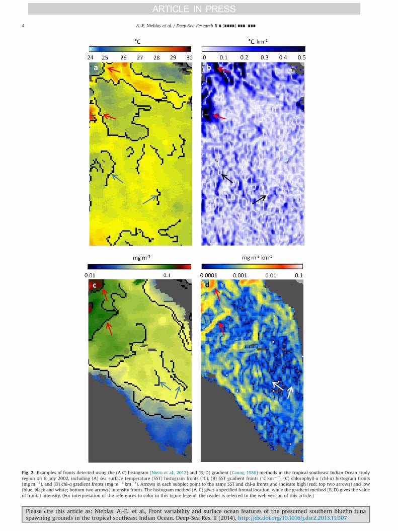
Fig. 2. Examples of fronts detected using the (A C) histogram (Nieto et al., 2012) and (B, D) gradient (Canny, 1986) methods in the tropical southeast Indian Ocean studyregion on 6 July 2002, including (A) sea surface temperature (SST) histogram fronts (1C), (B) SST gradient fronts (1C km�1), (C) chlorophyll-a (chl-a) histogram fronts(mg m�3), and (D) chl-a gradient fronts (mg m�3 km�1). Arrows in each subplot point to the same SST and chl-a fronts and indicate high (red; top two arrows) and low(blue, black and white; bottom two arrows) intensity fronts. The histogram method (A, C) gives a specified frontal location, while the gradient method (B, D) gives the valueof frontal intensity. (For interpretation of the references to color in this figure legend, the reader is referred to the web version of this article.)






Yukinawa and Miyabe, 1984; Nishikawa et al., 1985; Yukinawa andKoido, 1985; Yukinawa, 1987; Davis et al., 1990), is taken as theregion between 111S and 201S, 1101E and 1231E, and offshore of the200 m isobath (Box 1, Fig. 1). A coastal subregion of this area isdefined as being inshore of the 200 m isobath (Box 2, Fig. 1). We alsoinvestigate the front activity in the supposed transport corridor ofSBT larvae and juveniles along the Western Australian coastline inthe southern area of the study region from Exmouth to Geraldton(221S–301S, 1091E–1151E; Box 3, Fig. 1). Spectral energy plots of frontoccurrence and intensity are calculated separately for all subregionsto investigate the harmonics of each time-series. To isolate inter-annual variations, time-series of front occurrence and intensity ineach subregion are low-pass filtered using an 18-month Hammingwindow. Lagged correlations are investigated between the filteredtime-series of monthly front indices and the SOI, DMI, and windstress curl.

3. Results

Relative to the rest of the Indian Ocean, the offshore spawningregion of SBT (Box 1, Fig. 1) has low values of chl-a and EKE (Fig. 3),is seasonally stable in terms of SST (Fig. 4a), has relatively high SSTand chl-a front occurrence, and relatively low SST and chl-a frontintensity (Fig. 3). The offshore subregion has SSTs greater than241C throughout the year, even at its most southern limit (201S;Figs. 3 and 4a). Chl-a is low within the offshore spawning region,but relatively high concentrations are found throughout the yearin most of the coastal subregion and just south of the spawningregion at 221S and 251S–261S (Fig. 3 and 4b). The tropical southeastIndian Ocean is an area of low EKE (Fig. 3c), suggesting that themesoscale eddy activity here is weak. Within this area, EKE is

highest in the coastal subregion between 141S–181S (Fig. 4c). Eddyactivity is also found in the offshore subregion just south of theIndonesian archipelago (111S–121S) throughout the year, and inthe southern subregion south of 261S from May to October(Fig. 3c). Front occurrence for both SST and chl-a is high in thetropical southeast Indian Ocean, the Arabian Sea, and the Mozam-bique Channel (Fig. 3d, f). In the tropical southeast Indian Ocean,front occurrence is highest throughout the coastal subregion alongthe northwest coast of Australia (Fig. 4d, f; Fig. 5). Front occurrenceis concentrated in the offshore spawning region from 141S to 201Sand in the northern part of the southern subregion (221S–251S;Fig. 4d, f). SST front intensity is low throughout the Indian Ocean,with exceptions in the southwest Indian Ocean at the AgulhasReturn Current and Subtropical Convergence Zone and near thesouthwestern tip of Australia (Fig. 3e). Chl-a fronts are found onlywhere chl-a is found (Fig. 3b, g). SST and chl-a front intensity isrelatively low in the offshore subregion compared to adjacentregions, both along the coast and to the south (191S–301S;Figs. 3 and 4e, g).

3.1. Spatial variability of front occurrence in the tropical southeastIndian Ocean

Monthly climatologies of SST front occurrence clearly show thatthe Indo-Australian region and the Arabian Sea have the highestand most persistent SST front occurrence of the Indian Ocean(Supplemental 1). A close-up of Supplemental 1 of the tropicalsoutheast Indian Ocean is given in Fig. 5. In the Indo-Australianregion, a permanent SST front is observed from Exmouth toBroome, closely following the coastline (1141E–1261E; Fig. 5).A semi-permanent SST front is also observed in the Joseph BonaparteGulf from May to October (Fig. 5). From April to September,

Fig. 3. Maps of mean values for the months of the spawning season (September–April) of the southern bluefin tuna, Thunnus maccoyii, in the Indian Ocean (301N–451S,201E–1401E) for sea surface temperature (SST; 1C), (B) chlorophyll-a (chl-a; mg m�3), (C) Eddy Kinetic Energy (cm2 s�2), (D) SST front occurrence (%), (E) SST front intensity(1C km�1), (F) chl-a front occurrence (%), and (G) chl-a front intensity (mg m�3 km�1). Boxes indicate the three subregions investigated in this study, as in Fig. 1.






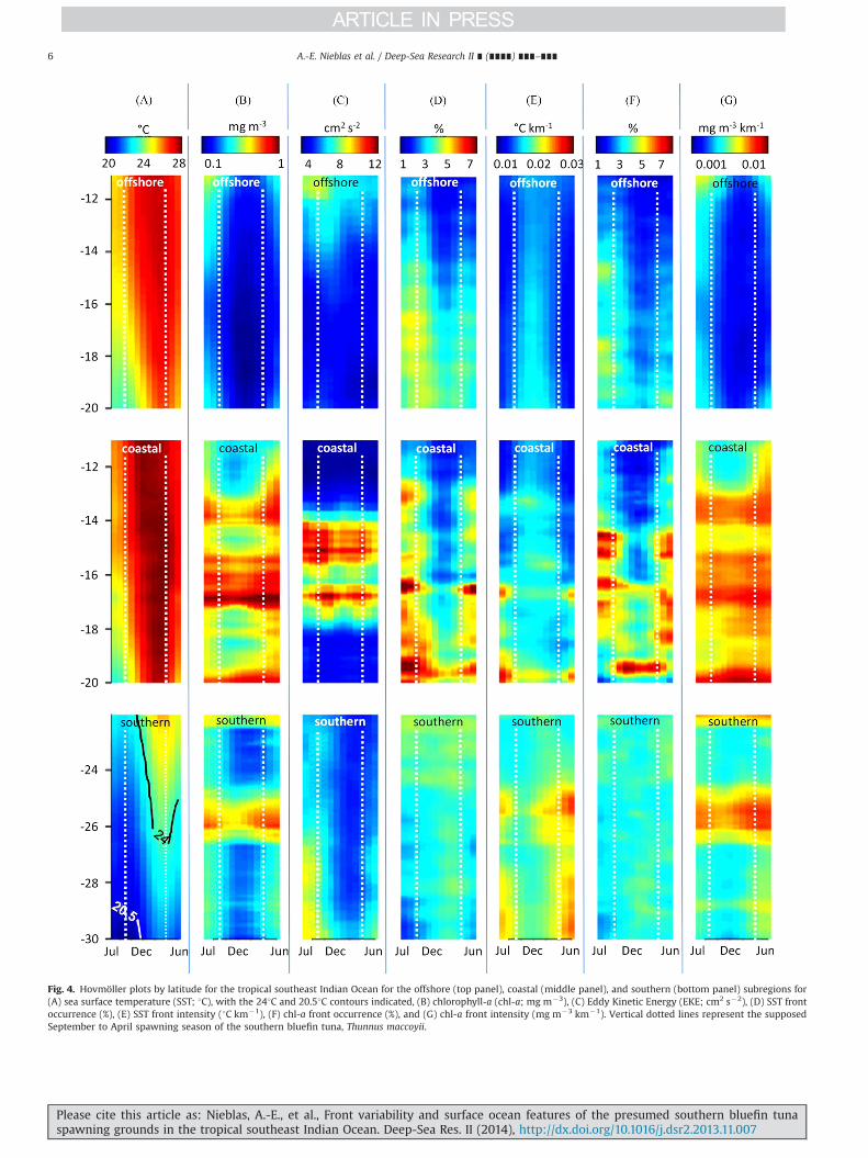
Fig. 4. Hovmöller plots by latitude for the tropical southeast Indian Ocean for the offshore (top panel), coastal (middle panel), and southern (bottom panel) subregions for(A) sea surface temperature (SST; 1C), with the 241C and 20.51C contours indicated, (B) chlorophyll-a (chl-a; mg m�3), (C) Eddy Kinetic Energy (EKE; cm2 s�2), (D) SST frontoccurrence (%), (E) SST front intensity (1C km�1), (F) chl-a front occurrence (%), and (G) chl-a front intensity (mg m�3 km�1). Vertical dotted lines represent the supposedSeptember to April spawning season of the southern bluefin tuna, Thunnus maccoyii.






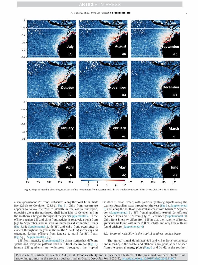
a semi-permanent SST front is observed along the coast from SharkBay (261S) to Geraldton (28.51S; Fig. 5). Chl-a front occurrenceappears to follow the 200 m isobath in the coastal subregion,especially along the northwest shelf from May to October, and inthe southern subregion throughout the year (Supplemental 2). In theoffshore region, SST and chl-a front activity is relatively strong fromJuly to September, and is seen as numerous disconnected fronts(Fig. 5a–f; Supplemental 2a–f). SST and chl-a front occurrence isevident throughout the year in the south (201S–301S), increasing andextending further offshore from January to April for SST fronts(Fig. 5g–j; Supplemental 2g–j).

SST front intensity (Supplemental 3) shows somewhat differentspatial and temporal patterns than SST front occurrence (Fig. 5).Intense SST gradients are widespread throughout the tropical

southeast Indian Ocean, with particularly strong signals along thewestern Australian coast throughout the year (Fig. 3e, Supplemental3) and along the southwest Australian coast from March to Septem-ber (Supplemental 3). SST frontal gradients extend far offshorebetween 151S and 301S from July to December (Supplemental 3).Chl-a front intensity differs from SST in that the majority of frontalgradients are found within the 200 m isobath, and very little of this isfound offshore (Supplemental 4).

3.2. Seasonal variability in the tropical southeast Indian Ocean

The annual signal dominates SST and chl-a front occurrenceand intensity in the coastal and offshore subregions, as can be seenfrom the spectral energy plots (Figs. 6 and 7c, d). In the southern

Fig. 5. Maps of monthly climatologies of sea surface temperature front occurrence (%) in the tropical southeast Indian Ocean (51S–301S, 851E–1301E).






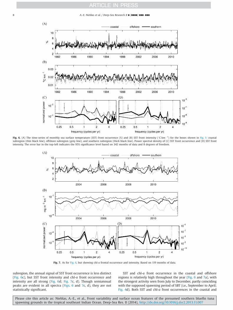
subregion, the annual signal of SST front occurrence is less distinct(Fig. 6c), but SST front intensity and chl-a front occurrence andintensity are all strong (Fig. 6d; Fig. 7c, d). Though semiannualpeaks are evident in all spectra (Figs. 6 and 7c, d), they are notstatistically significant.

SST and chl-a front occurrence in the coastal and offshoreregions is relatively high throughout the year (Fig. 6 and 7a), withthe strongest activity seen from July to December, partly coincidingwith the supposed spawning period of SBT (i.e., September to April;Fig. 4d). Both SST and chl-a front occurrences in the coastal and

Fig. 6. (A) The time-series of monthly sea surface temperature (SST) front occurrence (%) and (B) SST front intensity (1C km�1) for the boxes shown in Fig. 1: coastalsubregion (thin black line), offshore subregion (grey line), and southern subregion (thick black line). Power spectral density of (C) SST front occurrence and (D) SST frontintensity. The error bar in the top-left indicates the 95% significance level based on 342 months of data and 8 degrees of freedom.

Fig. 7. As for Fig. 6, but showing chl-a frontal occurrence and intensity. Based on 119 months of data.






offshore subregions are in phase, but differ substantially in magni-tude (Fig. 4d, f). In contrast, SST front occurrence in the southernsubregion shows low seasonal variability (Figs. 6c, 7c); with aslight peak from December to April south of 251S for SST fronts(Fig. 4d).

Patterns in front intensity differ between SST and chl-a fronts(Fig. 3e, g; Fig. 4e, g). Whereas SST front occurrence and intensityappear related (e.g., Fig. 3d, e), chl-a front occurrence and intensityare not (Fig. 3e, f). SST front intensity is inversely related to SSTfront occurrence, so regions of high SST front occurrence are oftenregions of low SST front intensity (e.g., the tropical southeastIndian Ocean and the Arabian Sea) with the opposite occasionallybeing true (e.g., low SST front occurrence but high SST frontintensity in the Agulhas Return Current/Subtropical ConvergenceZone; Fig. 3d, e). SST front intensity peaks from September to Aprilfor the offshore and coastal subregions, when SST front occurrencein these subregions is lowest, and is highest from March toSeptember in the southern subregion when SST front occurrencehere is lowest (Fig. 4d–g). In contrast, spatio-temporal patterns ofchl-a front intensity do not appear related to chl-a front occur-rence, but, rather, to chl-a itself (Figs. 3 and 4b, f, g). Both chl-aconcentration and chl-a front intensity are low in the offshorezone, remarkably high and stable throughout the year for thecoastal zone, and moderately strong throughout the year in thesouthern subregion (Fig. 4b, g; Fig. 8d).

3.3. Relationship to regional wind variability

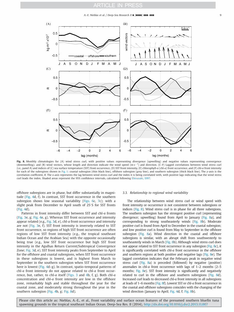
The relationship between wind stress curl or wind speed withfront intensity or occurrence is not consistent between subregions orindices (Fig. 8). Wind stress curl is in phase for all three subregions.The southern subregion has the strongest positive curl (representingdivergence; upwelling) found from April to January (Fig. 8a), andcorresponding to strong southeasterly winds (Fig. 8b). Moderatepositive curl is found from April to December in the coastal subregion;and low positive curl is found from May to September in the offshoresubregion (Fig. 8a). Wind direction in the coastal and offshoresubregions is similar, with an abrupt shift from southwesterly tosoutheasterly winds in March (Fig. 8b). Although wind stress curl doesnot appear related to SST front occurrence in any subregion (Fig. 8c), itis significantly correlated with chl-a front occurrence in the offshoreand southern regions at both positive and negative lags (Fig. 8e). Thelagged correlation indicates that the February peak in negative windstress curl (Fig. 8a) is preceded (followed) by negative (positive)anomalies in chl-a front occurrence with lags of 1–2 months (2–5months; Fig. 8e). SST front intensity is significantly and negativelyrelated to curl in the offshore and southern subregions (Fig. 8d).Increased curl leads to decreased chl-a front intensity in all subregionsat leads of 1–6months (Fig. 8f). Lowest SSTor chl-a front occurrence inthe coastal and offshore subregions coincides with the changing of thewind direction (January to April; Fig. 4d, f; Fig. 8b).

Fig. 8. Monthly climatologies for (A) wind stress curl, with positive values representing divergence (upwelling) and negative values representing convergence(downwelling); and (B) wind vectors, whose length and direction indicate the wind speed (m s�1) and direction. (C–F) Lagged correlations between wind stress curl(i.e., panel A) and indices of (C) sea surface temperature (SST) front occurrence, (D) SST front intensity, (E) chlorophyll-a (chl-a) front occurrence, and (F) chl-a front intensityfor each of the subregions shown in Fig. 1: coastal subregion (thin black line), offshore subregion (grey line), and southern subregion (thick black line). The y-axis is thecorrelation coefficient, R. The x-axis represents the lag between wind stress curl and the index it is being correlated with, with positive lags indicating that the wind stresscurl leads the index. Shaded areas represent the 95% confidence intervals, calculated following Ebisuzaki, 1997.






3.4. Interannual variability and relationship to large-scale climateindices

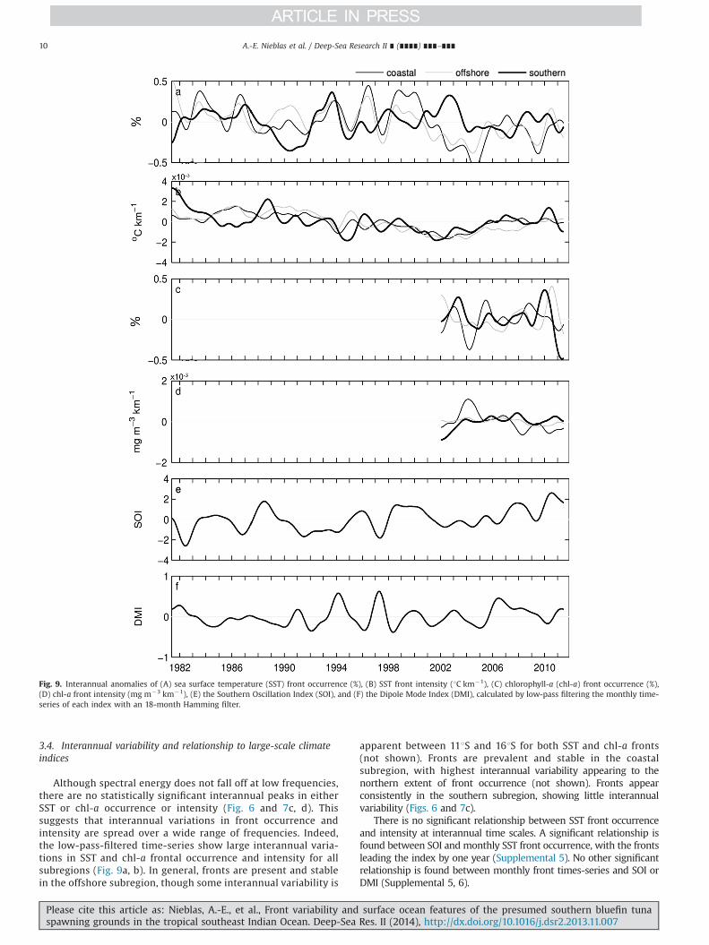
Although spectral energy does not fall off at low frequencies,there are no statistically significant interannual peaks in eitherSST or chl-a occurrence or intensity (Fig. 6 and 7c, d). Thissuggests that interannual variations in front occurrence andintensity are spread over a wide range of frequencies. Indeed,the low-pass-filtered time-series show large interannual varia-tions in SST and chl-a frontal occurrence and intensity for allsubregions (Fig. 9a, b). In general, fronts are present and stablein the offshore subregion, though some interannual variability is

apparent between 111S and 161S for both SST and chl-a fronts(not shown). Fronts are prevalent and stable in the coastalsubregion, with highest interannual variability appearing to thenorthern extent of front occurrence (not shown). Fronts appearconsistently in the southern subregion, showing little interannualvariability (Figs. 6 and 7c).

There is no significant relationship between SST front occurrenceand intensity at interannual time scales. A significant relationship isfound between SOI and monthly SST front occurrence, with the frontsleading the index by one year (Supplemental 5). No other significantrelationship is found between monthly front times-series and SOI orDMI (Supplemental 5, 6).

Fig. 9. Interannual anomalies of (A) sea surface temperature (SST) front occurrence (%), (B) SST front intensity (1C km�1), (C) chlorophyll-a (chl-a) front occurrence (%),(D) chl-a front intensity (mg m�3 km�1), (E) the Southern Oscillation Index (SOI), and (F) the Dipole Mode Index (DMI), calculated by low-pass filtering the monthly time-series of each index with an 18-month Hamming filter.






4. Discussion

4.1. Characteristics of the tropical southeast Indian Ocean SBTspawning region

This study examines front variability and ocean dynamics in theregion where SBT spawning has been observed and the adjacentareas. We show that the main spawning region is characterised bystable surface conditions: continuously warm SST, low EKE, andlow chl-a. However, we find high variability in the occurrence ofSST and chl-a fronts, though these are of relatively low intensitycompared to the surrounding regions and the Indian Ocean on thewhole. The putative SBT spawning season partly coincides with theseasonal peak in front occurrence and completely coincides withthe seasonal peak in front intensity in the offshore spawningground. We show that front activity in the spawning region hasdistinct annual signals, and some interannual variability.

Little is known about the spawning season of SBT, but unlike othertemperate tunas that migrate and spawn in distinct seasons, there issome evidence that SBT spawn throughout the year in the tropicalsoutheast Indian Ocean, primarily during winter months (Caton, 1991;Farley and Davis, 1998; Schaefer, 2001). All tuna species spawn intropical and subtropical oligotrophic waters, generally with a mini-mum SST of about 241C, but observed to be as low as 20.51C (Alemanyet al., 2010). This temperature threshold has been usedto define the geographical limits of the tuna spawning habitat(e.g., Schaefer, 2001; Muhling et al., 2011), and we confirm that thisthreshold is maintained throughout the year in the tropical southeastIndian Ocean, as far south as 201S. This is unlike the spawning regionsof other species of bluefin tuna, which can be cooler than 241Cdepending on the season (Schaefer, 2001; Locarnini et al., 2010). Thisstable temperature is partly due to the poleward-flowing LeeuwinCurrent, which opposes upwelling-favourable winds (McCreary et al.,1986) and maintains warm water at higher latitudes than othereastern boundary currents (Pearce, 1991). This feature indicates thatthe tropical southeast Indian Ocean region is conducive to spawningthroughout the year, potentially explaining the lack of distinctseasonality of SBT spawning migrations (Schaefer, 2001). The timingof SBT spawning migrations may also be due to variability in SBTwinter foraging habitat (e.g., Patterson et al., 2008; Evans et al., 2012).

Fish recruitment and survival success is traditionally linked toocean processes that promote productivity but do not force strongadvection or turbulence that is deleterious to larval development(e.g., the optimal environmental window; Cury and Roy, 1989).EKE activity in this region clearly shows that the majority of thespawning ground (121S–201S) is a region of low eddy activity,indicating stable and retentive characteristics (Figs. 3 and 4c). Thisis in contrast to the regions directly to the north (61S–121S) and tothe south (261S–301S; Figs. 3 and 4c), which are known as regionsof relatively large eddy activity (Pearce and Griffiths, 1991; Fengand Wijffels, 2002; Ogata and Masumoto, 2010).

Satellite data reveal that the offshore SBT spawning region isremarkably low in chl-a, especially in comparison to coastal seas(0.1 mg m�3; Fig. 3b), in concurrence with spawning regions of theAtlantic bluefin tuna (Thunnus thynnus; Druon et al., 2011). Themigration from highly productive feeding grounds to highlyoligotrophic spawning grounds is a common reproductive strategyamongst tuna species (Bakun and Broad, 2003; Muhling et al.,2010) perhaps used to avoid predation during the larval stageregardless of poor larval feeding conditions (Bakun and Broad,2003). This strategy may be used because, in oligotrophic regions,tuna larvae are near the top of the size spectrum. So, although thelarval growth rate may be relatively low due to low food avail-ability, there is also much lower predatory pressure, which leadsto increased larval survival overall in comparison to spawning inareas where adult tunas feed (Bakun and Broad, 2003).

Though the SBT larval stage is short (�20 days; Jenkins andDavis 1990), feeding incidence of tuna in the tropical southeastIndian Ocean region is closely related to food density (Young andDavis, 1990), and ocean features that concentrate food sources,such as the fronts observed in this study, could be important tolarval survival. In fact, the spawning region is shown to be a regionof relatively high chl-a fronts. Our results indicate that thespawning ground is a region of high occurrences of both SST andchl-a fronts, but low front intensity, relative to the rest of theIndian Ocean. This suggests that SBT spawning takes place in aregion where fronts are present and capable of entraining theavailable food resources, but do not have an intensity that wouldbe associated with strong vertical advection (Denman and Gargett,1983) or productivity that is high enough to support predation.

4.2. Variability of front occurrence

The driving mechanism of the fronts in the offshore subregionis relatively weak in terms of its ability to form temperaturegradients, but persistent and high-intensity fronts are found in thecoastal and southern subregions. The permanent and semi-permanent fronts that we find (Fig. 5, Supplemental 1, 3) areconsistent in location and persistence with those described byBelkin et al. (2009) who attribute them to upwelling and fresh-water flux. However, upwelling in this region is weak over thecontinental shelf and occurs under only particular conditionsduring the southeast monsoon (Wyrtki, 1962). In addition, frontshere are out of phase with the summer monsoon (December toMarch) when precipitation in the region is high (Wyrtki, 1961; Quand Meyers, 2005), though strong coastal fronts are found inregions of high riverine outflow (Fig. 5, Supplemental 3). Tidalmixing may also play an important role (Belkin and Cornillon,2003; Belkin and O'Reilly, 2009), but its influence is beyond thescope of the present study and was not investigated here. It is alsopossible that the nearshore fronts that are observed in the coastalsubregion are due to variability in local circulation; however,monitoring of nearshore currents is limited in this region so it isnot possible to show this directly.

The dominant dynamical feature in the southern subregion isthe LC, which flows poleward just off the coast with peak strengthin winter (Smith et al., 1991). It is related to the Indo-Australianbasin through the ITF (Nof et al., 2002; Feng et al., 2005) and theEastern Gyral Current (Qu and Meyers, 2005). Although there is adebate about whether the ITF outflow has a pathway southwardalong the northwest Australian coast (e.g., Nof et al., 2002;Domingues et al., 2007), both the ITF and the LC transportrelatively warm and fresh water (Cresswell and Golding, 1980;Meyers et al., 1995; Potemra, 2001; Liu et al., 2005; Sprintall et al.,2009) that likely produces strong thermal gradients with thecooler waters in the southern and coastal subregions. Chl-a frontsare also numerous, but their intensity appears to be related to theamount of chl-a in the region (Fig. 4b, g), which is higher in thecoastal subregion due to coastal dynamics, including riverineoutflow and upwelling. Chl-a fronts in the oligotrophic offshorespawning ground have low intensity.

Wind stress curl appears to explain some variability in theseasonal chl-a front formation in the offshore and coastal sub-regions. Chl-a fronts are negatively related to wind stress curl inthe southern region, where upwelling-favourable winds are domi-nant, but opposed by the LC for large portion of the year (McCrearyet al., 1986). This potentially suppresses front formation thatwould otherwise occur due to upwelling. Our results concur withstudies that show high front occurrence during periods of lowwind, as low winds can mask thermal fronts due to mixing of thesurface skin (e.g., Katsaros and Soloviev, 2004). Variation of winddirection may be an important driver of front occurrence for those






regions that are influenced by the seasonal monsoon. Changes inwind direction are known to affect circulation, upwelling anddownwelling (Pond and Pickard, 1983), and can therefore con-tribute to the formation of fronts.

Interannual variability of SST front occurrence is related to SOI,with the fronts leading the SOI by one year for the offshoresubregion (Fig. 9, Supplemental 5), indicating that the mechanismdriving SST front formation here also precedes ENSO. Oceandynamics in the tropical southeast Indian Ocean are known tobe influenced by both ENSO and IOD (Meyers, 1996; Saji et al.,1999). A recent study showed that negative IOD leads El Ninoevents in the Indian Ocean by one year, indicated by warming andstrong wind anomalies (Izumo et al., 2010) that could potentiallycontribute to thermal front formation.

To our knowledge, this paper is the first to characterise theoceanographic characteristics of the only region where SBT havebeen observed to spawn. It is a region of complex currents andlarge variability of upper-ocean conditions. Here, we investigatefronts detected from SST and chl-a gradients, which could be usedin the future to help characterise potential spawning habitat. Ouranalysis indicates that front dynamics in the tropical southeastIndian Ocean are complex, and we suggest several possibilities forthe linkages to regional and remote ocean dynamics. Other typesof fronts important for ecology, including salinity and nutrientfronts, are not examined here, but may also be prevalent featuresin this region. We suggest that studies on the distribution andvariability of SBT larvae on the spawning ground and theirassociation with ocean features are of major importance.

Acknowledgments

AEN was funded by CSIRO Wealth from the Oceans NationalResearch Flagship and a travel grant from l'Institut Français deRecherche pour l'Exploitation de la Mer. BMS was supported bythe Australian Climate Change Science Program, funded jointly bythe Department of Climate Change and Energy Efficiency andCSIRO. We would like to thank Igor Belkin, Steve Teo, PeterCornillon, Karen Evans, Toby Patterson, and 6 anonymousreviewers for their constructive comments on earlier versions ofthis manuscript. We also thank Toby Patterson, Jessica Farley, andCraig Proctor for their early support and interest in this project.

Appendix A. Supplementary material

Supplementary data associated with this article can be found inthe online version at http://dx.doi.org/10.1016/j.dsr2.2013.11.007.

References

Alemany, F., Quintanilla, L., Velez-Belchí, P., García, A., Cortés, D., Rodríguez, J.M.,Fernández de Puelles, M.L., González-Pola, C., López-Jurado, J.L., 2010. Char-acterization of the spawning habitat of Atlantic bluefin tuna and related speciesin the Balearic Sea (western Mediterranean). Prog. Oceanogr. 86, 1-2), 2010, 21–38. CLimate Impacts on Oceanic TOp Predators (CLIOTOP) – CLIOTOP, CLIOTOPInternational Symposium.

Alvain, S., Moulin, C., Dandonneau, Y., Bréon, F., 2005. Remote sensing of phyto-plankton groups in case 1 waters from global SeaWiFS imagery. Deep-Sea Res. I52 (11), 1989–2004.

Bakun, 1996. Patterns in the Ocean: Ocean Processes and Marine PopulationDynamics. University of California Sea Grant, in Cooperation with Centro deInvestigaciones Biologicas de Noroeste, San Diego, California, USA, and La Paz,Baja California Sur, Mexico.

Bakun, A., Broad, K., 2003. Environmental 'loopholes' and fish population dynamics:comparative pattern recognition with focus on El Niño effects in the Pacific.Fish. Oceanogr. 12 (4/5), 458–473.

Belkin, I.M., Cornillon, P., 2003. SST fronts of the Pacific coastal and marginal seas.Pac. Oceanogr. 1 (2), 90–113.

Belkin, I.M., Cornillon, P.C., Sherman, K., 2009. Fronts in large marine ecosystems.Prog. Oceanogr. 81 (1–4), 223–226.

Belkin, I.M., O'Reilly, J.E., 2009. An algorithm for oceanic front detection inchlorophyll and SST satellite imagery. J. Mar. Syst. 78 (3), 319–326.

Bentamy, A., Quilfen, Y., Gohin, F., Grima, N., Lenaour, M., Servain, J., 1996.Determination and validation of average field from ERS-1 scatterometermeasurements. Glob. Atmos. Ocean Syst. 4, 1–29.

Bray, N., Bray, N.A., Wijffels, S.E., Chong, J.C., Fieux, M., Hautala, S., Meyers, G.,Morawitz, W.M.L., 1997. Characteristics of the Indo-Pacific throughflow in theeastern Indian Ocean, GRL WOCE Indian Ocean issue. Geophys. Res. Lett. 24,2569–2572.

Canny, J., 1986. A computational approach to edge detection. IEEE Trans. PatternAnal. Mach. Intell. PAMI 8 (6), 679–698.

Caton, A.E., 1991. Review of Aspects of Southern Bluefin Tuna: Biology, Populationand Fisheries. In: Interactions of Pacific Tuna Fisheries, vol. 2, pp. 181–350.

Cayula, J.-F., Cornillon, P., 1992. Edge detection algorithm for SST images. J. Atmos.Ocean. Technol. 9, 67–80.

Clarke, A.J., Liu, X., 1994. Interannual sea level in the northern and eastern IndianOcean. J. Phys. Oceanogr. 24 (6), 1224–1235.

Cresswell, G., Golding, T., 1980. Observations of a south-flowing current in thesoutheastern Indian Ocean. Deep-Sea Res. A 27 (6), 449–466.

Cresswell, G.R., Frische, A., Peterson, J., Quadfasel, D., 1993. Circulation in Timor Sea.J. Geophys. Res. 98, 14379–14389.

Cury, P., Roy, C., 1989. Optimal environmental window and pelagic fish recruitmentsuccess in upwelling areas. Can. J. Fish. Aquat. Sci. 46 (4), 670–680.

Davis, T.L.O., Jenkins, G.J., Young, J.W., 1990. Patterns of horizontal distribution ofthe larvae of southern bluefin (Thunnus maccoyii), and other tuna in the IndianOcean. J. Plankton Res. 12, 1295–1314.

Denman, K.L., Gargett, A.E., 1983. Time and space scales of vertical mixing andadvection of phytoplankton in the upper ocean. Limnol. Oceanogr. 28 (5),801–815.

Domingues, C.A., Maltrud, M.E., Wijffels, S.E., Church, J.A., Tomczak, M., 2007.Simulated Lagrangian pathways between the Leeuwin Current System and theupper-ocean circulation of the southeast Indian Ocean. Deep-Sea Res. II 54 (8–10), 797–817.

Druon, J.N., Fromentin, J.-M., Aulanier, F., Heikkonen, J., 2011. Identification offeeding and spawning habitats of Atlantic bluefin tuna. Mar. Ecol. Prog. Ser. 439,223–240.

Ebisuzaki, W., 1997. A method to estimate the statistical significance of a correla-tion when the data are serially correlated. J. Clim. 10, 2147–2153.

Evans, K., Patterson, T.A., Reid, H., Harley, S.J., 2012. Reproductive schedules insouthern bluefin tuna: are current assumptions appropriate? PLoS One 7 (4),e34550. (doi:34510.31371/journal.pone.0034550).

Farley, J.H., Davis, T.L.O., 1998. Reproductive dynamics of southern bluefin tuna,Thunnus maccoyii. Fish. Bull. 96, 223–236.

Feng, M., Meyers, G., 2003. Interannual variability in the tropical Indian Ocean: atwo-year time-scale of Indian Ocean Dipole. Deep-Sea Res. II 50 (12–13),2263–2284.

Feng, M., Meyers, G., Pearce, A., Wijffels, S., 2003. Annual and interannual variationsof the Leeuwin Current at 321S. J. Geophys. Res. 108 (C11), 3355. 3310.1029/2002JC001763.

Feng, M., Wijffels, S., 2002. Intraseasonal variability in the South Equatorial Currentof the East Indian Ocean. J. Phys. Oceanogr. 32, 265–277.

Feng, M., Wijffels, S., Godfrey, S., Meyers, G., 2005. Do eddies play a role in themomentum balance of the Leeuwin Current? J. Phys. Oceanogr. 35,964–975.

Garcia, A., Alemany, F., Velez-Belchí, P., Lopez Jurado, J.L., Cortés, D., de la Serna, J.M.,González Pola, C., Rodríguez, J.M., Jansá, J., Ramírez, T., 2003. Characterisation ofthe bluefin tuna spawning habitat off the Balearic archipelago in relation to keyhydrographic features and associated environmental conditions. Collect. Vol.Sci. Papers ICCAT 58 (2), 535–549.

Gordon, A.L., Fine, R.A., 1996. Pathways of water between the Pacific and IndianOceans in the Indonesian seas. Nature 379, 146–149.

Izumo, T., Vialard, J., Lengaigne, M., de Boyer Montegut, C., Behera, S.K., Luo, J.-J.,Cravatte, S., Masson, S., Yamagata, T., 2010. Influence of the state of the IndianOcean Dipole on the following year's El Niño. Nat. Geosci., 3; , pp. 168–172.

Jenkins, G.P., Davis, T.L.O., 1990. Age, growth rate, and growth trajectory determinedfrom otolith microstructure of southern bluefin tuna Thunnus maccoyii larvae.Mar. Ecol. Prog. Ser. 63, 93–104.

Jia, F., Wu, L., Lan, J., Qiu, B., 2011. Interannual modulation of eddy kinetic energy inthe southeast Indian Ocean by Southern Annular Mode. J. Geophys. Res. 116,C02029. (doi:02010.01029/02010JC006699).

Kahru, M., Håkansson, B., Rud, O., 1995. Distributions of the sea surface tempera-ture fronts in the Baltic Sea as derived from satellite imagery. Cont. Shelf Res. 15(6), 663–679.

Katsaros, K.B., Soloviev, A.V., 2004. Vanishing horizontal sea surface temperaturegradients at low wind speeds. Bound.-Layer Meteorol. 112, 381–396.

Liu, Y., Feng, M., Church, J., Wang, D., 2005. Effect of salinity on estimatinggeostrophic transport of the Indonesian Throughflow along the IX1 XBT section.J. Oceanogr. 61 (4), 795–801.

Locarnini, R.A., Mishonov, A.V., Antonov, J.I., Boyer, T.P., Garcia, H.E., Baranova, O.K.,Zweng, M.M., Johnson, D.R., 2010. World Ocean Atlas 2009. In: Levitus, S. (Ed.),Temperature, vol. 1; 2010, p. 24. (NOAA Atlas NESDIS 71, 184).

Mariani, P., MacKenzie, B.R., Iudicone, D., Bozec, A., 2010. Modelling retention anddispersion mechanisms of bluefin tuna eggs and larvae in the northwestMediterranean Sea. Prog. Oceanogr. 86 (1–2), 45–58.




http://refhub.elsevier.com/S0967-0645(13)00446-3/sbref1






















































http://dx.doi.org/3310.1029/2002JC001763

http://dx.doi.org/3310.1029/2002JC001763







































McCreary, J.P., Shetye, S.R., Kundu, P.K., 1986. Thermohaline forcing of easternboundary currents, with application to the circulation off the west coast ofAustralia. J. Mar. Res. 44, 71–92.

Meyers, G., 1996. Variation of Indonesian throughflow and the El Nino-SouthernOscillation. J. Geophys. Res. 101 (C5), 12255–12263.

Meyers, G., Bailey, R.J., Worby, A.P., 1995. Geostrophic transport of the Indonesianthroughflow. Deep-Sea Res. I 42, 1163–1174.

Muhling, B.A., Lamkin, J.T., Roffer, M.A., 2010. Predicting the occurrence of Atlanticbluefin tuna (Thunnus thynnus) larvae in the northern Gulf of Mexico: buildinga classification model from archival data. Fish. Oceanogr. 19 (6), 526–539.

Muhling, B.A., Lee, S.K., Lamkin, J.T., Liu, Y., 2011. Predicting the effects of climatechange on bluefin tuna (Thunnus thynnus) spawning habitat in the Gulf ofMexico. ICES J. Mar. Sci. 68 (6), 1051–1062.

Nieto, K., Demarcq, H., McClatchie, S., 2012. Mesoscale frontal structures in theCanary Upwelling System: new front and filament detection algorithms appliedto spatial and temporal patterns. Remote Sens. Environ. 123, 339–346.

Nishikawa, Y., Honma, M., Ueyanagi, S., Kikawa, S., 1985. Average distribution oflarvae of oceanic species of scombrid fishes, 1956-1981. Far Seas Fish. Res. Lab.S Ser. 12, 1–99.

Nof, D., Pichevin, T., Sprintall, J., 2002. “Teddies” and the origin of the LeeuwinCurrent. J. Phys. Oceanogr. 32, 2517–2588.

Ogata, T., Masumoto, Y., 2010. Interactions between mesoscale eddy variability andIndian Ocean dipole events in the southeastern tropical Indian Ocean—casestudies for 1994 and 1997/1998. Ocean Dyn. 60, 717–730.

Patterson, T.A., Evans, K., Carter, T.I., Gunn, J.S., 2008. Movement and behaviour oflarge southern bluefin tuna (Thunnus maccoyii) in the Australian regiondetermined using pop-up satellite archival tags. Fish. Oceanogr. 17 (5),352–367.

Pearce, A., 1991. Eastern boundary currents of the southern hemisphere. J. R. Soc.West. Aust. 74, 35–45.

Pearce, A.F., Griffiths, R.W., 1991. The mesoscale structure of the Leeuwin Current: acomparison of laboratory models and satellite imagery. J. Geophys. Res. 96 (C9),16739–16757.

Pond, S., Pickard, G.L., 1983. Introductory Dynamical Oceanography. PergamonPress, Oxford.

Potemra, J.T., 2001. Contribution of equatorial Pacific winds to southern tropicalIndian Ocean Rossby waves. J. Geophys. Res. 106 (C2), 2407–2422.

Qu, T., Meyers, G., 2005. Seasonal variation of barrier layer in the southeasterntropical Indian Ocean. J. Geophys. Res. 110 (C11003), 25. (doi:11010.11029/12004JC002816).

Saji, N.H., Goswami, B.N., Vinayachandran, P.N., 1999. A dipole mode in the tropicalIndian Ocean. Nature 401, 360–363.

Sathyendranath, S., Platt, T., Horne, E., Harrison, W., Ulloa, O., Outerbridge, R.,Hoepffner, N., 1991. Estimation of new production in the ocean by compoundremote sensing. Nature 353, 129–133.

Schaefer, K.M., 2001. Reproductive biology of tunas. In: Block, B.A., Stevens, E.D.(Eds.), Tuna: Physiology, Ecology, and Evolution. Academic Press, San Diego,pp. 225–270.

Shingu, C., 1970. Studies relevant to distribution and migration of southern bluefintuna. Bull. Far Seas Res. Lab. 3, 57–113.

Smith, R.L., Huyer, A., Godfrey, J.S., Church, J.A., 1991. The Leeuwin Current offWestern Australia, 1986–1987. J. Phys. Oceanogr. 21, 323–345.

Sprintall, J., Gordon, A.L., Murtugudde, R., Susanto, R.D., 2000. A semiannual IndianOceanforced Kelvin wave observed in the Indonesian seas in May 1997. J.Geophys. Res. 105, 17217–19476.

Sprintall, J., Wijffels, S.E., Molcard, R., Jaya, I., 2009. Direct estimates of theIndonesian Throughflow entering the Indian Ocean: 2004–2006. J. Geophys.Res. 114, C07001. 07010.01029/02008JC005257.

Stegmann P.M. and Ullman D.S., Variability in chlorophyll and sea surfacetemperature fronts in the Long Island Sound outflow region from satelliteobservations. J. Geophys. Res-Oceans, 109(C7), 2004.

Trenberth, K.E., 1984. Signal versus noise in the Southern Oscillation. Mon. WeatherRev. 112 (2), 326–332.

Ueyanagi, S., 1969. Observations on the distribution of tuna larvae in the Indo-Pacific Ocean with emphasis on the delineation of the spawning areas of thealbacore, Thunnus alalunga. Bull. Far Seas Fish. Res. Lab. 2, 177–254.

Ullman, D.S., Cornillon, P.C., 1999. Satellite–derived sea surface temperature frontson the continental shelf off the northeast US coast. J. Geophys. Res.-Oceans 104(C10), 23459–23478.

Ullman, D.S., Cornillon, P.C., 2000. Evaluation of front detection methods forsatellite derived SST data using in situ observations. J. Atmos. Ocean. Technol.17 (12), 1667–1675.

Ullman, D.S., Cornillon, P.C., 2001. Continental shelf surface thermal fronts in winteroff the northeast US coast. Cont. Shelf Res. 21 (11), 1139–1156.

Wijffels, S., Meyers, G., 2004. An intersection of oceanic waveguides: variability inthe Indonesian Throughflow region. J. Phys. Oceanogr. 34, 1232–1253.

Wijffels, S.E., Meyers, G., Godfrey, J.S., 2008. A 20-yr average of the IndonesianThroughflow: regional currents and the Interbasin Exchange. J. Phys. Oceanogr.38, 1965–1978.

Wyrtki, K., 1961. Physical Oceanography of the Southeast Asian Waters, ScientificResults of Marine Investigations of the South China Sea and the Gulf ofThailand. NAGA Report 2. Scripps Institution of Oceanography, La Jolla, CA,pp. 1–225.

Wyrtki, K., 1962. The upwelling in the region between Java and Australia during thesoutheast monsoon. Aust. J. Mar. Freshw. Res. 13 (3), 217–225.

Wyrtki, K., 1987. Indonesian Through Flow and the associated pressure gradient.J. Geophys. Res. 92 (C12), 12941–12946.

Yonemori, T., Morita, J., 1978. Report on 1977 Research Cruise of the R/V ShoyoMaru. Distribution of Tuna and Billfishes Larvae and Oceanographic Observa-tion in the Eastern Indian Ocean, October–December, 1977. Report of theResearch Division, Fishery Agency of Japan, pp. 1–48.

Young, J.W., Davis, T.L.O., 1990. Feeding ecology of larvae of southern bluefin,albacore and skipjack tunas (Pisces: Scombridae) in the eastern Indian Ocean.Mar. Ecol. Prog. Ser. 61, 17–29.

Yu, Z., Potemra, J.T., 2006. Generation mechanism for the intraseasonal variability inthe Indo-Australian basin. J. Geophys. Res. 111, C01013. 01010.01029/02005JC003023.

Yukinawa, M., 1987. Report on 1986 research cruise of the R/V Shoyu Maru.Distribution of Tuna and Billfishes Larvae and Oceanographic Observation inthe Eastern Indian Ocean January–March 1985. Report of the Research Division,Fishery Agency of Japan, pp. 1–100.

Yukinawa, M., Koido, T., 1985. Report on 1984 research cruise of the R/V ShoyoMaru. Distribution of Tuna and Billfishes Larvae and Oceanographic Observa-tion in the Eastern Indian Ocean January–March, 1984. Report of the ResearchDivision, Fishery Agency of Japan, pp. 1–100.

Yukinawa, M., Miyabe, N., 1984. Report on 1983 Research Cruise of the R/V ShoyoMaru. Distribution of Tuna and Billfishes Larvae and Oceanographic Observa-tion in the Eastern Indian Ocean October–December, 1983. Report of theResearch Division, Fishery Agency of Japan, pp. 1–103.


























































http://dx.doi.org/07010.01029/02008JC005257


























http://dx.doi.org/01010.01029/02005JC003023

http://dx.doi.org/01010.01029/02005JC003023




Documents

Front variability and surface ocean features of the presumed southern bluefin tuna spawning grounds in the tropical southeast Indian Ocean