Frozen Soil Lateral Resistance for the Seismic Design of

Alaska D

epartment of Transportation &

Public Facilities A

laska University Transportation C

enter

Frozen Soil Lateral Resistance for the Seismic Design of Highway Bridge Foundations

Final Report

FHWA-AK-RD-12-23 INE/AUTC 12.34

Prepared By: Zhaohui “Joey” Yang Xiaoxuan Ge Benjamin Still Anthony Paris University of Alaska Anchorage, School of Engineering

December 2012

Alaska University Transportation Center Duckering Building Room 245 P.O. Box 755900 Fairbanks, AK 99775-5900

Alaska Department of Transportation Research, Development, and Technology Transfer 2301 Peger Road Fairbanks, AK 99709-5399

Prepared By:

REPORT DOCUMENTATION PAGE

Form approved OMB No.

Public reporting for this collection of information is estimated to average 1 hour per response, including the time for reviewing instructions, searching existing data sources, gathering and maintaining the data needed, and completing and reviewing the collection of information. Send comments regarding this burden estimate or any other aspect of this collection of information, including suggestion for reducing this burden to Washington Headquarters Services, Directorate for Information Operations and Reports, 1215 Jefferson Davis Highway, Suite 1204, Arlington, VA 22202-4302, and to the Office of Management and Budget, Paperwork Reduction Project (0704-1833), Washington, DC 20503 1. AGENCY USE ONLY (LEAVE BLANK) FHWA-AK-RD-12-23

2. REPORT DATE December 2012

3. REPORT TYPE AND DATES COVERED Final Report (08/01/2011-12/31/2012)

4. TITLE AND SUBTITLE Frozen Soil Lateral Resistance for the Seismic Design of Highway Bridge Foundations

5. FUNDING NUMBERS AUTC#510021 DTRT06-G-0011 T2-11-04

6. AUTHOR(S) Zhaohui “Joey” Yang, Xiaoxuan Ge, Benjamin Still, Anthony Paris 7. PERFORMING ORGANIZATION NAME(S) AND ADDRESS(ES) Alaska University Transportation Center P.O. Box 755900 Fairbanks, AK 99775-5900

8. PERFORMING ORGANIZATION REPORT NUMBER INE/AUTC 12.34

9. SPONSORING/MONITORING AGENCY NAME(S) AND ADDRESS(ES) Alaska Department of Transportation Research, Development, and Technology Transfer 2301 Peger Road Fairbanks, AK 99709-5399

10. SPONSORING/MONITORING AGENCY REPORT NUMBER FHWA-AK-RD-12-23

11. SUPPLENMENTARY NOTES 12a. DISTRIBUTION / AVAILABILITY STATEMENT No restrictions

12b. DISTRIBUTION CODE

13. ABSTRACT (Maximum 200 words) With recent seismic activity and earthquakes in Alaska and throughout the Pacific Rim, seismic design is becoming an increasingly important public safety concern for highway bridge designers. Hoping to generate knowledge that can improve the seismic design of highway bridges in Alaska, researchers from the University of Alaska plan to test a fixity depth approach and a lateral resistance (p-y) approach in seismic bridge design. Currently, the Alaska Department of Transportation and Public Facilities (ADOT&PF) utilizes soil lateral resistance in the seismic design of bridge pile foundations. Knowledge about lateral resistance of frozen soils, particularly seasonally frozen soils at shallow depths, will help improve pile foundation design in cold regions such as Alaska. Researchers Zhaohui Yang and Anthony Paris are conducting laboratory experiments to examine key mechanical parameters for the frozen soils used to construct the p-y curve for modeling frozen soils. Although there have been studies on the mechanical properties of frozen soils, existing studies were based on remolded, artificially frozen soil samples, which do not necessarily represent the soil in the field. How much impact these disturbances have on the frozen soil strength and stress-strain behavior is not clear. Additionally there is a lack of studies of the stress-strain behavior at small strains based on naturally frozen samples. Yang and Paris hope to fill this knowledge gap by providing key frozen soil parameters for typical Alaska soils. These key soil parameters, Yang and Paris claim, are needed for predicting the formation and location of plastic hinges, and internal loads in bridge pilings embedded in frozen soils during seismic loading. The team will use this developing knowledge to conduct a bridge design engineers workshop to discuss their findings and how to apply them in the seismic design of bridges. 14- KEYWORDS: Earthquake resistant design (Esdc), Bridge design (Esusb), Frozen soils (Rbespfh)

15. NUMBER OF PAGES 91 16. PRICE CODE

N/A 17. SECURITY CLASSIFICATION OF REPORT

Unclassified

18. SECURITY CLASSIFICATION OF THIS PAGE

Unclassified

19. SECURITY CLASSIFICATION OF ABSTRACT

Unclassified

20. LIMITATION OF ABSTRACT

N/A

NSN 7540-01-280-5500 STANDARD FORM 298 (Rev. 2-98) Prescribed by ANSI Std. 239-18 298-1

Notice This document is disseminated under the sponsorship of the U.S. Department of Transportation in the interest of information exchange. The U.S. Government assumes no liability for the use of the information contained in this document. The U.S. Government does not endorse products or manufacturers. Trademarks or manufacturers’ names appear in this report only because they are considered essential to the objective of the document.

Quality Assurance Statement The Federal Highway Administration (FHWA) provides high-quality information to serve Government, industry, and the public in a manner that promotes public understanding. Standards and policies are used to ensure and maximize the quality, objectivity, utility, and integrity of its information. FHWA periodically reviews quality issues and adjusts its programs and processes to ensure continuous quality improvement.

Author’s Disclaimer Opinions and conclusions expressed or implied in the report are those of the author. They are not necessarily those of the Alaska DOT&PF or funding agencies.

SI* (MODERN METRIC) CONVERSION FACTORS

APPROXIMATE CONVERSIONS TO SI UNITSSymbol When You Know Multiply By To Find Symbol

LENGTH in inches 25.4 millimeters mm ft feet 0.305 meters m yd yards 0.914 meters m mi miles 1.61 kilometers km

AREA in2 square inches 645.2 square millimeters mm2

ft2 square feet 0.093 square meters m2

yd2 square yard 0.836 square meters m2

ac acres 0.405 hectares ha mi2 square miles 2.59 square kilometers km2

VOLUME fl oz fluid ounces 29.57 milliliters mL gal gallons 3.785 liters L ft3 cubic feet 0.028 cubic meters m3

yd3 cubic yards 0.765 cubic meters m3

NOTE: volumes greater than 1000 L shall be shown in m3

MASS oz ounces 28.35 grams glb pounds 0.454 kilograms kgT short tons (2000 lb) 0.907 megagrams (or "metric ton") Mg (or "t")

TEMPERATURE (exact degrees) oF Fahrenheit 5 (F-32)/9 Celsius oC

or (F-32)/1.8

ILLUMINATION fc foot-candles 10.76 lux lx fl foot-Lamberts 3.426 candela/m2 cd/m2

FORCE and PRESSURE or STRESS lbf poundforce 4.45 newtons N lbf/in2 poundforce per square inch 6.89 kilopascals kPa

APPROXIMATE CONVERSIONS FROM SI UNITS Symbol When You Know Multiply By To Find Symbol

LENGTHmm millimeters 0.039 inches in m meters 3.28 feet ft m meters 1.09 yards yd km kilometers 0.621 miles mi

AREA mm2 square millimeters 0.0016 square inches in2

m2 square meters 10.764 square feet ft2

m2 square meters 1.195 square yards yd2

ha hectares 2.47 acres ac km2 square kilometers 0.386 square miles mi2

VOLUME mL milliliters 0.034 fluid ounces fl oz L liters 0.264 gallons gal m3 cubic meters 35.314 cubic feet ft3

m3 cubic meters 1.307 cubic yards yd3

MASS g grams 0.035 ounces ozkg kilograms 2.202 pounds lbMg (or "t") megagrams (or "metric ton") 1.103 short tons (2000 lb) T

TEMPERATURE (exact degrees) oC Celsius 1.8C+32 Fahrenheit oF

ILLUMINATION lx lux 0.0929 foot-candles fc cd/m2 candela/m2 0.2919 foot-Lamberts fl

FORCE and PRESSURE or STRESS N newtons 0.225 poundforce lbf kPa kilopascals 0.145 poundforce per square inch lbf/in2

*SI is the symbol for th International System of Units. Appropriate rounding should be made to comply with Section 4 of ASTM E380. e(Revised March 2003)

vi

TABLE OF CONTENTS

REPORT DOCUMENTATION PAGE .......................................................................................... iii

ACKNOWLEDGMENT OF SPONSORSHIP AND DISCLAIMER ........................................... iv

METRIC CONVERSION SHEET ..................................................................................................v

LIST OF FIGURES ....................................................................................................................... ix

LIST OF TABLES ....................................................................................................................... xiii

ACKNOWLEDGMENTS ........................................................................................................... xiv

ABSTRACT ...................................................................................................................................xv

EXECUTIVE SUMMARY ..............................................................................................................1

CHAPTER 1: INTRODUCTION ....................................................................................................2

1.1 BACKGROUND .................................................................................................................. 2

1.2 LITERATURE REVIEW ...................................................................................................... 3

1.2.1 Experimental Study of Frozen Soil Mechanical Properties ........................................... 3

1.2.2 Sampling Disturbance Effect on Mechanical Properties of Frozen Soils ...................... 3

1.2.3 Shear Wave Velocity in Frozen Soils ............................................................................. 4

1.3 PROBLEM STATEMENT .................................................................................................... 4

1.4 STUDY OBJECTIVE ........................................................................................................... 4

1. 5 SCOPE OF WORK .............................................................................................................. 5

CHAPTER 2: SAMPLING, MACHINING, AND TESTING PROCEDURES FOR FROZEN SOILS ..............................................................................................................................................6

2.1 INTRODUCTION ................................................................................................................ 6

2.2 SITE PREPARATION .......................................................................................................... 6

2.3 SAMPLING .......................................................................................................................... 7

vii

2.4 TRANSPORTATION ............................................................................................................ 8

2.5 STORAGE ............................................................................................................................ 8

2.6 MACHINING ....................................................................................................................... 9

2.7 CONDITIONING AND SOIL CLASSIFICATION ........................................................... 11

2.8 TESTING APPARATUS AND INSTRUMENTATION ..................................................... 14

CHAPTER 3: DATA AND OBSERVATIONS ..............................................................................16

3.1 SPECIMEN ORIENTATION ............................................................................................. 16

3.2 TYPICAL STRESS-STRAIN CURVES ............................................................................ 16

3.3 DATA INTERPRETATION ................................................................................................ 17

3.4 CHARACTERISTICS OF THAWED SOILS .................................................................... 21

3.5 OBSERVATIONS OF SPECIMEN FAILURE MODES .................................................... 22

CHAPTER 4: ANALYSIS AND DISCUSSION OF RESULTS ...................................................29

4.1 ULTIMATE COMPRESSIVE STRENGTH ...................................................................... 29

4.2 YIELD STRENGTH ........................................................................................................... 34

4.3 YOUNG’S MODULUS ...................................................................................................... 36

4.4 SHEAR WAVE VELOCITY............................................................................................... 37

4.5 ε50 AND STRAIN AT YIELD STRENGTH ....................................................................... 38

CHAPTER 5: CONCLUSION AND RECOMMENDATIONS ....................................................41

5.1 SUMMARY AND CONCLUSIONS .................................................................................. 41

5.2 RECOMMENDATIONS AND FUTURE RESEARCH .................................................... 42

REFERENCES ..............................................................................................................................43

viii

APPENDIX A: Stress-Strain Curves for Tested Specimens ..........................................................46

ix

LIST OF FIGURES

Figure 2.1 Installation of a temperature monitoring conduct at the Campbell Creek bridge site. .............................................................................................................................7

Figure 2.2 Sampling at the Campbell Creek Bridge Site (left) and the CRREL Permafrost Tunnel (right). ................................................................................................................8

Figure 2.3 A frozen soil sample being cut into an octagon with the wood jig by a band saw. …… .................................................................................................................................9

Figure 2.4 A frozen soil specimen in the special holding bit on the lathe. ............................ 11

Figure 2.5 Conditioning curves of two frozen soil specimens. .............................................12

Figure 2.6 Grain-size distribution of permafrost. ..................................................................13

Figure 2.7 Grain-size distribution of seasonally frozen soil. ................................................13

Figure 2.8 The Universal Testing Machine (UTM-100) with a temperature chamber and computer interface. ...................................................................................................14

Figure 2.9 An extensometer attached to the middle of a frozen soil specimen during loading. ...............................................................................................................................15

Figure 3.1 Frozen soil specimen orientation. ........................................................................16

Figure 3.2 Stress-strain curves for seasonally frozen soil. ....................................................17

Figure 3.3 Stress-strain curves for permafrost. .....................................................................17

Figure 3.4 Interpreting the yield strength. .............................................................................18

Figure 3.5 Interpreting Young’s modulus. .............................................................................19

Figure 3.6 Young’s modulus interpretation for specimen P4 H4 with small defect. .............19

Figure 3.7 Specimen P4 H4 with small defect at the center of one end. ...............................20

Figure 3.8 A vertically oriented naturally frozen soil cylinder with ice lenses: before testing (left) and after testing to 15% axial strain (right). ...................................................22

Figure 3.9 Seasonally frozen soil specimen C9 H4 (left) and C7 V1 (right). .......................22

Figure 3.10 Failure of specimen C2 H1 due to bending. ...............................................................23

Figure 3.11 Failure of specimen P4 V2 due to shearing. ...............................................................24

Figure 4.1 Ultimate compressive strength vs. temperature for seasonally frozen soil………….. ................................................................................................................................30

x

Figure 4.2 Ultimate compressive strength vs. temperature for permafrost. ..........................30

Figure 4.3 Ice wedges observed in the CRREL Permafrost Tunnel. .....................................31

Figure 4.4 Comparison of ultimate compressive strength with previous studies. .................31

Figure 4.5 Dry density vs. water content...............................................................................32

Figure 4.6 Ultimate compressive strength vs. dry density. ...................................................33

Figure 4.7 Ultimate compressive strength vs. water content. ...............................................34

Figure 4.8 Yield strength vs. ultimate strength for seasonally frozen soil. ...........................35

Figure 4.9 Yield strength vs. ultimate strength for permafrost. ............................................35

Figure 4.10 Yield strength vs. ultimate strength for both seasonally frozen soil and permafrost, and its comparison with a previous study. ..................................................................36

Figure 4.11 Young’s modulus vs. temperature. .........................................................................37

Figure 4.12 Shear wave velocity vs. temperature. ..................................................................38

Figure 4.13 ε50 vs. temperature................................................................................................38

Figure 4.14 ε50 vs. dry density. ................................................................................................39

Figure 4.15 Strain at yield strength vs. temperature. ...............................................................39

Figure 4.16 Strain at yield strength vs. dry density. ................................................................40

Figure A.1 Stress-strain curve for Specimen C1H1. ......................................................................46

Figure A.2 Stress-strain curve for Specimen C1V1. ......................................................................46








Figure A.10 Stress-strain curve for Specimen C4V3. ....................................................................50

Figure A.11 Stress-strain curve for Specimen C6H1. ....................................................................51

xi



















Figure A.30 Stress-strain curve for Specimen C10H1. ..................................................................60





Figure A.35 Stress-strain curve for Specimen C10V1. ..................................................................63




xii

Figure A.39 Stress-strain curve for Specimen P4H1. ....................................................................65


Figure A.41 Stress-strain curve for Specimen P4V1. ....................................................................66

















Figure A.58 Stress-strain curve for Specimen P11V1. ..................................................................74



xiii

LIST OF TABLES

Table 3.1. Representative soil parameters. .....................................................................................21

Table 3.2. Physical and Mechanical Properties of Frozen Soil Specimens ...................................25

xiv

ACKNOWLEDGMENTS

The research reported herein was supported by the Alaska University Transportation Center

(AUTC) and the State of Alaska Department of Transportation and Public Facilities under AUTC

Project #510021 and performed by the Department of Civil Engineering with the help of the

Department of Mechanical Engineering at the University of Alaska Anchorage (UAA).

Dr. Zhaohui Yang, Associate Professor of Civil Engineering, was the Principal Investigator.

Other authors of this report are Ms. Xiaoxuan Ge and Mr. Benjamin Still, both graduate students,

and Dr. Anthony Paris, Associate Professor of Mechanical Engineering, all from UAA’s School

of Engineering. The authors would like to express their thanks to Dr. Scott Hamel and Mr. Daniel

King for their assistance on the data acquisition system. Mr. Donald Richardson took part in

these experiments. We are thankful to former graduate students Mr. Xiaoyu Zhang and Mr. Qiang

Li from UAA for their assistance with field sampling.

xv

ABSTRACT

Frozen soils, especially seasonally frozen soils, have a significant effect on the seismic

performance of bridge pile foundations. To account for this effect, it is necessary to evaluate

frozen soils’ mechanical properties. This report focuses on obtaining the mechanical properties of

naturally frozen silty soils in Alaska. High-quality specimens of both permafrost and seasonally

frozen soil were prepared by block sampling and machining following a procedure designed to

minimize mechanical and thermal disturbances. Both horizontal and vertical specimens were

prepared to investigate the effect of specimen orientation. Unconfined compression tests were

performed at temperatures ranging from -0.7° to -11.6°C at a constant deformation rate that

corresponds to a strain rate of about 0.1%/s. This strain rate is equivalent to that expected in the

frozen soil during a design earthquake in Interior Alaska. Test results including soil

characteristics and mechanical properties (stress-strain curves, compressive strength, yield

strength, and modulus of elasticity) are presented and compared with data in the literature. The

impact of temperature, dry density, water content, and specimen orientation on mechanical

properties is discussed. These mechanical properties can be directly used to evaluate frozen soil

lateral resistance in the analyses of laterally loaded pile foundations during seismic or other

events in cold regions.

1

EXECUTIVE SUMMARY

This report describes the sampling, machining, conditioning, and unconfined compression

testing procedures used to determine the mechanical properties of naturally frozen soils in

Alaska—both seasonally frozen soil and permafrost—and presents the testing data and analyses

that resulted from that work. The main findings from this project are summarized below:

1. The ultimate compressive strength decreases with increasing temperature; it decreases

with increasing dry density, or increases with increasing water content. This trend for the

latter is clearer at lower temperatures. In addition, there is a correlation between yield

strength and ultimate compressive strength.

2. The Young’s modulus decreases with increasing temperature. The horizontal specimens

tend to have higher Young’s modulus, especially for permafrost. Similarly, the shear

wave velocity of frozen soils decreases with increasing temperature.

3. For permafrost, the ultimate strength of horizontal specimens is substantially higher than

that of vertical specimens at the same testing temperature. This strength anisotropy is

likely due to ice wedge formation commonly observed in permafrost.

4. The ultimate strength of naturally frozen soils is lower than that obtained from remolded

frozen soils.

5. Factors that affect the mechanical properties of frozen soils include temperature, water

content or dry density, specimen orientation, and soil type.

2

CHAPTER 1: INTRODUCTION

1.1 BACKGROUND

Frozen ground, including seasonally frozen soil and permafrost, occurs across the State of Alaska. A project titled “Seasonally frozen effects on the seismic response of highway bridges,” jointly funded by the Alaska University Transportation Center (AUTC) and the Alaska Department of Transportation and Public Facilities (ADOT&PF), Project #107014, 2007–2010 (PIs: Hulsey and Yang), showed that seasonally frozen soils significantly affect the seismic performance of bridges in Alaska. It was found that frozen soils not only alter overall bridge dynamic properties (i.e., fundamental period), but also affect the failure mechanisms of the bridge substructure system during lateral loads including earthquakes (Li et al. 2011). For example, the location and length of the plastic hinge formed on a bridge piling due to earthquake loading will be much different in winter than in summer; the internal loads of the pile will be different as well.

The location and length of the plastic hinge and the shear and bending moment are crucial parameters for the seismic design of bridge substructures. To predict and estimate those parameters accurately, Hulsey and Yang (2011) proposed two methods: the fixity depth approach and the lateral soil resistance (p-y) approach. The fixity depth approach is relatively simple and can only account for frozen soil conditions that have been studied. Past studies (e.g., Reese and Matlock 1956; McClelland and Focht 1958; Reese and Van Impe 2001) have shown that the p-y approach is versatile and provides a practical means for design. This approach can be applied in other frozen soil conditions if certain mechanical properties of the frozen soil are obtained. Crowther (1990) studied frozen soil resistance for creep analysis and developed p-y curves for laterally loaded piles embedded in layered frozen soil for short-term and long-term loading. For the bridge engineers to construct p-y curves for any frozen soil based on the recommended p-y curve (Hulsey and Yang 2011; Yang et al. 2012), key mechanical parameters including the unconfined compressive strength σm, the axial strain at which σm is achieved, and the axial strain ε50 at which 50% of σm is achieved are required.

These key mechanical parameters are not available for most frozen soils in Alaska. The parameters are sensitive to temperature and ice/water content, to soil type, and to sample-preparation method. To obtain these parameters reliably, the testing equipment must include a high-quality temperature chamber and a data-acquisition system that is sensitive to small and large strains. This project aims to fill the knowledge gap by providing these key frozen soil parameters for typical Alaskan soils.

3

1.2 LITERATURE REVIEW

1.2.1 Experimental Study of Frozen Soil Mechanical Properties

Frozen soil properties largely depend on temperature, ice/water content, strain rate, dry density, and soil type. Early studies (Sayles 1968; Sayles and Haines 1974) mainly focused on the creep behavior of frozen soils (sands, silts, and clays). Akili (1971) studied the stress-strain behavior and strength of frozen fine soils (clay and clayey silt) at varying strain rates. Sayles (1973) and Jones and Parameswaran (1983) studied the stress-strain behavior of frozen Ottawa sand. Watson et al. (1973) conducted a comprehensive study on the thaw settlement and strength of permafrost by using large permafrost core samples taken from the field.

Baker et al. (1982) found that low confining pressure (0 to 0.35 MPa) has little effect on the compressive strength or axial strain at failure. Vinson et al. (1983) conducted a comprehensive study on the dynamic elastic properties of naturally frozen silts from the Cold Regions Research and Engineering Laboratory (CRREL) Permafrost Tunnel, including both horizontally and vertically oriented specimens, by using cored specimens. They found little difference between the dynamic properties of horizontally and vertically oriented specimens, and confining pressure up to 500 MPa had little impact on the dynamic Young’s modulus. Zhu and Carbee (1984) carried out a uniaxial compression test program on remolded frozen Fairbanks silt under various deformation rates and studied the mechanical properties including uniaxial compressive strength. Most existing studies, except Watson et al. (1973) and Vinson et al. (1983), were based on remolded, artificially frozen soil samples, which do not necessarily represent the field conditions.

1.2.2 Sampling Disturbance Effect on Mechanical Properties of Frozen Soils

Sample disturbance has important effects on the stress-strain and strength behavior of unfrozen soils; its impact on frozen soils is equally important. The disturbance of frozen samples, including sublimation, evaporation, and thermal disturbance, may affect their strength and deformation properties. Soil structure may be completely altered if the sample is thawed, remolded, and then refrozen.

Baker (1976) conducted a comprehensive review of the transportation, preparation, and storage of frozen soil samples for laboratory testing. Radd and Wolfe (1979) compared the shear strength of field-frozen samples and laboratory-frozen samples and found that the field-frozen samples are weaker than the laboratory-frozen samples at all tested temperatures. In identifying six major variables that could affect the strength of frozen soils, Radd and Wolfe (1979) determined that the most important ones include freezing conditions, strain rate, and sample

4

orientation and size. Knutsson (1981) also showed that frozen soil shear strength properties are sensitive to the sample preparation method.

1.2.3 Shear Wave Velocity in Frozen Soils

Cox et al. (2012) developed relationships between the mean shear wave velocity (Vs) over the top 30 m of the subsurface (referred to as Vs30) and surficial geologic units, permitting seismic site classification throughout Fairbanks, Alaska, for both frozen and unfrozen conditions. Based on their results, it was determined that much of the city of Fairbanks is on NEHRP Site Class D material when unfrozen. When the near-surface material is frozen, its Vs increased significantly (700% on average). However, this drastic increase in stiffness was typically limited to the top 1–2 m of the subsurface, and only resulted in an increase in site class from NEHRP D to NEHRP C at 3 of the 16 sites retested during the winter.

Based on LeBlanc et al. (2004), permafrost is not clearly highlighted by a sharp increase in velocities; rather a gradual increase in velocity marks the passage between the frozen active layer and permafrost. The seismic velocity variation in permafrost is associated with three principal factors: (1) ground temperature, (2) ice content, and (3) unfrozen water content. Maximum shear wave velocities occur at where the ice content of permafrost is probably highest.

1.3 PROBLEM STATEMENT

The soil lateral resistance approach is widely used in the seismic design of bridge pile foundations, and is used by. Knowledge on the lateral resistance of frozen soils, particularly seasonally frozen soils at shallow depths, is needed for designing pile foundations in cold-region areas including Alaska. Although studies have been conducted on the mechanical properties of frozen soils, most of these studies have been based on remolded, artificially frozen soil samples, which do not necessarily represent field conditions. Moreover, how much impact the disturbances have on frozen soil strength and stress-strain behavior is not clear. There is a lack of study on soil stress-strain behavior at large strain rates using naturally frozen samples, and there is no information on the dependency of frozen soil properties at large strains on specimen orientation.

1.4 STUDY OBJECTIVE

The objective of this project is to evaluate quantitatively the mechanical properties of undisturbed, naturally frozen silt for the seismic design of pile foundations embedded in frozen soils.

5

1. 5 SCOPE OF WORK

The scope of this study includes the following tasks:

1. Sample naturally frozen soils at specified sites (the CRREL Permafrost Tunnel for permafrost, the Campbell Creek Bridge Site for seasonally frozen soil).

2. Transport the frozen samples in a portable freezer.

3. Machine the samples to 4 in. height by 2 in. diameter specimens with minimal mechanical and thermal disturbance.

4. Condition the specimens at selected temperatures at least 24 hours before testing.

5. Perform an unconfined compression test on all specimens at a constant deformation rate compatible with that of earthquake loading and gather stress-versus-strain data.

6. Obtain the physical properties of soil through standard soil tests.

7. Process and analyze test data.

8. Provide comments and recommendations for design of bridge pile foundations in cold regions.

6

CHAPTER 2: SAMPLING, MACHINING, AND TESTING PROCEDURES FOR FROZEN SOILS

2.1 INTRODUCTION

The quality of the naturally frozen soil sample depends on the type of frozen soil that has been sampled, the in situ thermal condition at the time of sampling, the sampling method, the transportation and storage procedures, and the specimen machining procedure prior to testing. Methods for sampling, transportation, storage, and machining of frozen soils were proposed by Baker (1976). Baker et al. (1982) investigated the end effects during unconfined compression tests using different platens. Ebel (1985) discussed the aspect ratio of frozen soil cylinders and end effects during uniaxial compression testing. De Re et al. (2003) proposed triaxial testing methods and equipment for constant strain rate control in testing frozen soils.

Many research programs have been carried out over the years; however, not many have tackled naturally frozen soils with high strain rates during compression tests, which present many difficulties due to a specimen’s non-uniformity. This chapter refines methods and tools used in the sampling and specimen machining to minimize evaporation, sublimation, and thermal disturbance of naturally frozen specimens.

2.2 SITE PREPARATION

Two sites from which to take frozen soil samples were chosen: the CRREL Permafrost Tunnel at Fox, Alaska, and the North Fork of Campbell Creek Bridge in Anchorage, Alaska, with the former representing permafrost and the later representing seasonally frozen soil. At the Campbell Creek Bridge site a steel pipe was drilled into the ground to facilitate monitoring of ground temperature and depth of the seasonally frozen soil (see Figure 2.1). Monitoring data help determine the sampling depth and natural temperature of the frozen soil. Based on observations of ground temperature from this study and a previous study (Li et al. 2011) at this site, seasonally frozen soil can reach 5 feet deep, and its temperature ranges from -1 to -10 °C.

7

Figure 2.1 Installation of a temperature monitoring conduct at the Campbell Creek bridge site.

2.3 SAMPLING

Frozen soil is very stiff. A STIHL carbide-chain chainsaw was used to cut out blocks of frozen soil approximately 1 ft3 (see Figure 2.2). Where electricity is readily available or where exhaust is a concern (such as the permafrost tunnel), an electric chainsaw is used, but at more remote locations, including bridges sites, a gas-powered chainsaw is needed. The chainsaws worked well in frozen silt. However, when small pieces of gravel were encountered in gravelly soils, the blade dulled quickly resulting in increased cutting time and melting of the soil. To extract soil blocks, a square was cut in the ground with the chainsaw and a wedge was pounded into one side of the chainsaw cut, which snapped the bottom of the block. Typically, the bottom broke irregularly and was trimmed in a cold room later. Pulling the block out of the ground can be difficult. We typically tried to angle the blade of the chainsaw slightly to make the block smaller at the base and used nail pullers to pull out the blocks. The orientation of the frozen soil block is important, and we noted which side was the surface and if the surface had any inclination from the horizontal plane.

8

Figure 2.2 Sampling at the Campbell Creek Bridge Site (left) and the CRREL Permafrost Tunnel (right).

2.4 TRANSPORTATION

After the frozen soil blocks were extracted from the ground, they were wrapped in cellophane and put in a polyurethane bag with some snow to help minimize moisture loss. Air was extruded from the bag before it was sealed to help prevent sublimation. The samples were placed in a portable freezer run by a car battery to minimize thermal disturbance while being transported to the cold room for storage.

Due to the distance of the CRREL Permafrost Tunnel from the University of Alaska Anchorage (UAA) Cold Room we took more samples than the portable freezer is able to carry. The rest of the samples were placed in a RocketBox on top of the vehicle for transportation to Anchorage. The temperatures were warm for December, but well below 0°C.

2.5 STORAGE

Frozen block samples were placed in the cold room in their polyurethane bag. The bags were inspected for holes and places of wear during transportation. If any bag had been compromised, the sample was resealed in another polyurethane bag. It is important to keep the temperature of the block samples as close to the in situ temperature as possible during storage. Temperatures in

9

a typical cold room can fluctuate substantially, and insulating the samples can help reduce this fluctuation.

2.6 MACHINING

The ASTM standard D7300-06 describes a standard test method for laboratory determination of strength properties of frozen soils at a constant strain rate. It recommends using a cylindrical frozen soil specimen of certain dimension for performing the unconfined compression test. Experience indicates that consistent creep and strength results can be obtained when the height-to-diameter ratio is at least three to two (Ebel 1985), so we decided to use specimens of 4 in. height by 2 in. diameter.

Frozen soil blocks can be large and irregular. A band saw in a cold room is a great way to cut through these blocks. Good-quality metal cutting blades can be used to cut through frozen silt, sand, and even the occasional piece of gravel, although cutting gravel dulls the cutting surface substantially. The outer inch or two of the block is generally considered heat-affected and trimmed off the block. We trimmed the blocks into vertically and horizontally oriented rectangular prisms of 3 in. by 3 in. by 4.5 in. To save time on lathing, we also trimmed the long corners to make octagon-shaped prisms, using a wood jig (see Figure 2.3).

Figure 2.3 A frozen soil sample being cut into an octagon with the wood jig by a band saw.

10

After the specimens were cut into octagons, they were lathed into cylinders using a special holding bit. Using a lathe in a cold room for machining frozen soils presents certain problems. Most lathes are designed to work in room temperatures near 20°C, but the cold room is well below freezing, so the gears and moving parts of the lathe need to be cleaned, and cold-weather grease needs to be applied instead of the factory grease. The shavings of the frozen soil specimen work their way into the gears and moving parts, creating unnecessary wear. Using a shop vacuum during the machining process helps to keep soil particles out of the gears.

A special holding bit to turn the frozen soil specimen is needed, as seen in Figure 2.4. Ideally, a carbide tip cutter should be used for the lathe. Standard cutters dull quickly and begin affecting the soil with heat. During the initial lathing, as much as 100/1000 in. was trimmed at a time until the specimen was within 1/4 in. of the required diameter. During final trimming, no more than 15/1000 in. was trimmed at a time, typically reduced to 5/1000 in. during the final turn. After the specimen was turned to the 2 in. diameter, we used a four-jawed chuck, a standard holding bit, to face both ends using a framing square to make sure both sides were parallel to each other and perpendicular to the cylinder surface. Facing the frozen soil specimen is very important, and a sharp cutter is essential for performing this task. While facing, we took off no more than 15/1000 in. In the final pass, no more than 5/1000 in. was taken off the face. The face was inspected for any defects or inconsistencies before the specimen was wrapped in cellophane, labeled, and put into a polyurethane bag to prevent sublimation for storage. Testing was typically done within one week of specimen completion.

11

Figure 2.4 A frozen soil specimen in the special holding bit on the lathe.

2.7 CONDITIONING AND SOIL CLASSIFICATION

Frozen soil mechanical properties are very sensitive to temperature and other factors. We planned to test the specimens at a range of temperatures. A small adjustable freezer was used to condition the specimens to a specific temperature. Thermocouples were placed on the specimens, and then the specimens were insulated fully and placed in the freezer for a minimum of 24 hours. The rest of the freezer was filled with ice in bags to help minimize any temperature variation. Figure 2.5 presents an example of the conditioning curves. The variation of temperature during the final stage of conditioning was less than 0.1°C.

12

Figure 2.5 Conditioning curves of two frozen soil specimens.

Before compression testing, several more steps are necessary. Photos were taken of the different aspects of the frozen soil cylinder including both ends. Notes were taken about the visual classification of the specimen including location, size, and distribution of ice, and larger grains of soil. The specimen was given a frozen-soil classification according to ASTM standard D4083-89. All samples contained visible ice lenses and, with few exceptions, were classified as V based on the appropriate ice descriptor. Both the length and diameter of the specimen were measured. The sample was transported to the Universal Testing Machine (UTM-100) in a cooler conditioned to -10°C.

Several sieve analysis and hydrometer tests were conducted for both the permafrost and seasonally frozen soil. Figures 2.6 and 2.7 present the respective grain-size distribution of the permafrost and seasonally frozen soil. Both soils contained large amounts of fines. The permafrost is classified as silt, while the seasonally frozen soil is classified as sandy organic silt with several specimens being classified as peat because of their highly organic nature.

0 500 1000 1500 2000 2500 3000-6

-5.8

-5.6

-5.4

-5.2

-5

-4.8

-4.6

-4.4

-4.2

-4

Time, min

Tem

pera

ture

, ° C

C10H1C10V1

13

Figure 2.6 Grain-size distribution of permafrost.

Figure 2.7 Grain-size distribution of seasonally frozen soil.

0

10

20

30

40

50

60

70

80

90

100

0.00010.0010.010.11

Perc

ent F

iner

(%)

Grain Diameter (mm)

Sieve AnalysisHydrometer Test

0%

10%

20%

30%

40%

50%

60%

70%

80%

90%

100%

0.0010.010.11

Perc

ent F

iner

(%)

Grain Diameter (mm)

Sieve AnalysisHydrometer Test

14

2.8 TESTING APPARATUS AND INSTRUMENTATION

The unconfined compression test was completed by the UTM-100 with the 3k pancake load cell (see Figure 2.8). The UTM-100 has a temperature chamber that can maintain the temperature as cold as -17°C. A fan was installed in the chamber to improve air circulation, help maintain a more uniform temperature environment, and minimize thermal disturbance of the frozen soil specimen.

Figure 2.8 The Universal Testing Machine (UTM-100) with a temperature chamber and computer interface.

It is recommended that lubricated platens be used whenever possible in the unconfined compression and creep testing of frozen soils (Ebel 1985). The lubricated platen consists of a circular sheet of 0.8 mm thick latex membrane, attached to the loading face of a steel platen with a 0.5 mm thick layer of high-vacuum silicon grease. The steel platens are polished stainless steel disks about 10 mm larger than the specimen diameter (ASTM D7300-06, 2006).

Displacement control was used during the compression test. A constant deformation rate corresponding to a strain rate of about 0.1%/s was applied for all tests. Note this strain rate is equivalent to the strain rate level expected in the frozen soil during a design earthquake in Interior Alaska (Yang and Zhang 2012). As the latex sheets and grease layers compress under load, the axial strain of the specimen should be measured using an MTS extensometer installed near the center of the specimen (see Figure 2.9). A load cell was used to measure axial load and,

15

hence, stress on the specimen. The extensometer and load cell were calibrated before use in these experiments. 9237 cDAQ system was used to record data.

Figure 2.9 An extensometer attached to the middle of a frozen soil specimen during loading.

16

CHAPTER 3: DATA AND OBSERVATIONS

3.1 SPECIMEN ORIENTATION

During seismic loading, the pile with its supported superstructure swings back and forth; hence, the main loading direction is horizontal. Traditionally, soil specimens, particularly bored soil samples, are obtained from a borehole perpendicular to the ground surface. To investigate whether the orientation of a soil specimen in reference to the ground surface has any impact on the soil mechanical properties, both vertical and horizontal specimens were prepared and tested. As illustrated in Figure 3.1, a vertical specimen (identified by V) indicates that its axis is perpendicular to the ground surface, and a horizontal specimen (identified by H) indicates that its axis is parallel to the ground surface. At least one vertical and one horizontal specimen were prepared from the center portion of the same block for comparison. All specimens are labeled by their sampling site and orientation. For example, C2 H1 indicates that this is #1 horizontal specimen prepared from block #2 taken from the Campbell Creek Bridge site (seasonally frozen soil); similarly, P2 V1 indicates that this is #1 vertical specimen prepared from block #2 taken from the Permafrost Tunnel (permafrost).

Figure 3.1 Frozen soil specimen orientation.

3.2 TYPICAL STRESS-STRAIN CURVES

A majority of the specimens were loaded to an axial strain of at least 15%. However, for safety reasons, some tests were terminated due to excessive bending of the specimen, likely caused by non-uniform density and the asymmetrical mechanical property of the specimen. Figure 3.2 and Figure 3.3 show typical stress-strain curves for seasonally frozen soil and

17

permafrost, respectively. As shown in Figure 3.2, some specimens demonstrated a peak in the stress-strain curve (for example, C2 H1), and most others showed a strain-hardening behavior.

Figure 3.2 Stress-strain curves for seasonally frozen soil.

Figure 3.3 Stress-strain curves for permafrost.

3.3 DATA INTERPRETATION

The stress-strain curves obtained for a specimen can be used to interpret other important physical parameters such as ultimate strength, yield strength, Young’s modulus, and ε50.

0 0.02 0.04 0.06 0.08 0.1 0.12 0.14 0.16 0.18 0.20

1

2

3

4

5

6

Axial Strain

Stre

ss (M

pa)

C2V1 Temp.= -11.4°C

C2H1 Temp.= -5.8°C

C7V1 Temp.= -5.8°C

C6H4 Temp.= -2.9°C

C6V4 Temp.= -2.9°C

0 0.05 0.1 0.15 0.20

1

2

3

4

5

6

Axial Strain

Stre

ss (M

pa)

P6H2 Temp.=-4.5°C

P9V4 Temp.=-7.5°C

P4H4 Temp.=-1.0°C

P4V3 Temp.=-1.0°C

18

Most specimens were taken to over 15% strain, but we considered 2% strain to be failure. The ultimate compressive strength σm refers to the stress corresponding to 2% axial strain on the stress-stain (σ-ε) curve or the peak strength if a peak occurs prior to 2% strain. All peaks occurred before 2% strain. The strain correlating to 50% of the ultimate strength is referred to as ε50.

The yield strength σy is the stress at which yield is initiated. It is well known that soils including frozen soils exhibit plastic behavior at very small strains. Figure 3.4 illustrates how yield strength was determined in this study. The beginning phase of the stress-strain curve, whose trend line has an r2 value larger than 0.95, was considered the linear portion. After this portion, obvious yielding can be observed. The maximum stress in this linear portion was interpreted as the yield strength.

Figure 3.4 Interpreting the yield strength.

Young’s modulus E is the slope of the stress-strain curve at very small strains. It is observed that the linear portion on the stress-strain curve typically occurs at strains less than 0.00015, but this varies from specimen to specimen. At least four data points with small strain values were fitted to a line, and the slope of the line was taken as Young’s modulus (see Figure 3.5).

0 0.002 0.004 0.006 0.008 0.01 0.012 0.014 0.016 0.018 0.020

2

4

6

8

Axial Strain

Stre

ss (M

Pa)

r2 = 0.9519

σy

19

Figure 3.5 Interpreting Young’s modulus.

Interpreting Young’s modulus did not always work out as nicely as shown in Figure 3.5. For example, the stress-strain curve of Specimen P4 H4 began with a gradual slope before turning into a steep slope, as seen in Figure 3.6. It was found later that the initial gradual slope of the stress-strain curve was caused by a defect in the specimen, a small bump in the center as seen in Figure 3.7. The first three data points were ignored during the interpretation of Young’ modulus for this specimen.

Figure 3.6 Young’s modulus interpretation for specimen P4 H4 with small defect.

0 0.00002 0.00004 0.00006 0.00008 0.00010 0.000120

0.1

0.2

0.3

0.4

0.5

Axial Strain

Str

ess

(MP

a)

C11 V2Curve Fit

σ = 4811εr2 = 0.9822E = 4811 MPa

0.00005 0.0001 0.00015 0.0002 0.00025 0.00030

0.2

0.4

0.6

Axial Strain

Str

ess (

MP

a)

P4 H4Curve Fit

σ = 2233.8ε - 0.1714r² = 0.9985E= 2234 MPa

20

Figure 3.7 Specimen P4 H4 with small defect at the center of one end.

The shear wave velocity (Vs) was calculated using the following equations based on shear modulus (G), Poisson’s ratio (ν), and the soil density (ρ); E represents Young’s modulus of the frozen soil. Kaplar (1969) reported that values of Poisson's ratio for frozen soils as computed from average values of E (longitudinal vibrations) and G general range between 0.25 and 0.38, and the average values of Poisson’s ratio for the laboratory-frozen ice and natural lake ice, based on results obtained using longitudinal vibrations, range from 0.32 to 0.40. Poisson’s ratio of frozen soil was assumed to be 0.3 in this study.

𝐺 = 𝐸2(1+𝜈)

(3.1)

𝑉𝑠 = �𝐺𝜌

(3.2)

21

3.4 CHARACTERISTICS OF THAWED SOILS

Standard soil tests, for example, liquid limit test, plastic limit test and specific gravity were conducted for thawed seasonally frozen soil and permafrost, respectively. Average test results of three specimens of each type of frozen soils are shown in Table 3.1. General range of Specific Gravity (GS) for silt is 2.65~2.70. As shown in Table 3.1, GS in this study is slightly lower, which may be due to the relatively high organic content.

Table 3.1. Representative soil parameters.

Soil Type Liquid Limit

Plastic Limit

Plasticity Index

Specific Gravity (GS)

Seasonally frozen soil (C)

47 44 3 2.44

Permafrost (P) 39 37 2 2.55

Forty-five seasonally frozen soil specimens (23 vertical and 22 horizontal) and twenty-three

permafrost specimens (14 vertical and 9 horizontal) were prepared. All specimens were classified

as ice-rich organic silty soils; their water content ranged from 62 to 225%, and their dry density

varied from 320 to 941 kg/m3. An unconfined compression test was carried out for these

specimens under a constant deformation rate corresponding to a strain rate of about 0.1%/s at

temperatures varying from -0.7° to -11.6°C. Average specific gravity GS in Table 3.1 was used to

calculate the degree of ice saturation (S) by the following equations:

e = (Gsρw/ρd)-1 (3.3)

S = (ωρwGs/ρIce)/e (3.4)

where GS is the specific gravity of the soil at 20°C, ρw is the mass density of water (1000 kg/m3), ω is the water content of the soil sample, ρd is the dry mass density of the soil sample (kg/m3), ρIce is the mass density of ice (917 kg/m3), e is the void ratio. As shown in Table 3.2, the degree of ice saturation ranges from 81.13% to 100% for all tested specimens.

Table 3.2 lists the physical and mechanical properties of these specimens. The ultimate strength of these specimens varies from 1.65 to 7.08 MPa, and the yield strength varies from 0.74

22

to 5.08 MPa. Young’s modulus ranges from 2.1 to 10.6 GPa, and the shear wave velocity (Vs) as interpreted from the shear modulus ranges from 800 to 1800 m/s.

3.5 OBSERVATIONS OF SPECIMEN FAILURE MODES

Small ice lenses were found throughout the specimens in both the permafrost and seasonally frozen soil and were distributed non-uniformly. Figure 3.8 shows a vertically oriented specimen before and after testing. Note the ice lenses presented in this specimen. It is believed that the distribution of ice lenses, among other factors, affects the specimen’s failure mode. The water content of seasonally frozen soil was mostly above 100%, but the amount of ice lenses observed did not correspond to the water content. For example, specimen C9 H4 has minimally visible ice (see Figure 3.9), but has water content of 225%; specimen C7 V1 has many visible ice lenses (see Figure 3.9), but has water content of 124%. This percentage is still considered high, but when compared with C9 H4, it is nearly half the water content.

Figure 3.8 A vertically oriented naturally frozen soil cylinder with ice lenses: before testing (left) and after

testing to 15% axial strain (right).

Figure 3.9 Seasonally frozen soil specimen C9 H4 (left) and C7 V1 (right).

23

Observations made during testing helped identify three failure modes: bulging, bending, and shearing, as can be seen in Figures 3.8, 3.10, and 3.11. No collapsing was observed in the specimens. In most cases, small cracks were observed around pieces of rock or ice lenses on the surface of specimens.

Figure 3.10 Failure of specimen C2 H1 due to bending.

24

Figure 3.11 Failure of specimen P4 V2 due to shearing.

25

Table 3.2 Physical and Mechanical Properties of Frozen Soil Specimens

Specimen ID

Water Content ω (%)

Frozen Bulk

Density (kg/m3)

Dry Density

ρd (kg/m3)

Organic Content

(%)

Test Temperature

T (°C)

Ultimate Strength

σm (MPa)

Strain at σm (%)

ε50 (%)

Yield Strength σy (MPa)

Strain at Yield

Strength (%)

Young’s Modulus E (MPa)

Vs

(m/s) Saturation

(%)

C1 H1[1] 120 1254 570 18.5 -7 4.889 1.954 0.087 3.186 0.145 4706 1201 97.33

C1 V1 103 1302 642 35.5 -2.5 2.153 1.974 0.081 1.738 0.204 3366 997 97.86

C1 V2 86 1452 780 10.7 -6.3 3.99 N/A[3] N/A[3] 3.414 N/A[3] N/A[3] N/A[3] 100

C2 H1[1] 127 1254 551 21.6 -6 3.935 0.803 0.083 3.214 0.202 3784 1077 98.57

C2 H2[1] 121 1269 574 20.5 -5.8 3.325 0.65 0.062 2.351 0.117 5035 1235 99.04

C2 V1 120 1276 580 21.5 -11.6 4.96 1.95 0.061 2.975 0.088 6806 1432 99.57

C2 V2 94 1343 691 30.5 -9 4.759 1.99 0.074 2.963 0.113 6275 1341 98.82

C2 V3 115 1273 592 20.4 -11.4 4.448 1.97 0.068 2.701 0.1 5501 1289 98.03

C4 V1 200 1109 370 49.2 -3.4 2.938 2.014 0.124 1.775 0.178 3275 1066 95.12

C4 V2 162 1167 442 33.3 -8.8 4.938 1.998 0.095 2.713 0.115 4598 1231 95.36

C4 V3 154 1177 463 38.6 -9.5 4.471 1.986 0.08 2.433 0.095 5230 1037 95.97

C5 H1 128 1230 539 22.8 -5.6 4.465 N/A[3] N/A[3] 4.115 N/A[3] N/A[3] N/A[3] 96.57

C5 H2 125 1251 555 22.3 -6.1 4.21 N/A[3] N/A[3] 3.588 N/A[3] N/A[3] N/A[3] 97.93

C6 H1[1] 155 1181 464 31.6 -6.5 4.794 1.975 0.068 2.119 0.052 7895 1603 96.85

C6 H2[1] 128 1237 543 13.7 -9.5 5.801 1.453 0.112 4.156 0.229 4140 1171 97.49

C6 H3[1] 205 1111 364 20.4 -2.6 3.008 1.828 0.093 1.97 0.162 3159 1046 95.64

C6 V1 183 1120 396 35.5 -7.7 4.039 1.987 0.09 3.239 0.239 4167 1196 94.34

C6 V2 192 1124 385 44.7 -7.2 4.254 1.851 0.111 3.23 0.246 3528 1099 95.71

C6 V4 136 1217 515 30.5 -2.7 2.279 2.01 0.11 1.508 0.196 2484 886 96.81

C7 H1[1] 170 1176 436 19 -5.8 5.031 0.455 0.058 4.098 0.142 6724 1483 98.41

26

Specimen ID


Frozen Bulk

Density (kg/m3)

Dry Density

ρd (kg/m3)

Organic Content

(%)

Test Temperature

T (°C)

Ultimate Strength

σm (MPa)

Strain at σm (%)

ε50 (%)


Strain at Yield

Strength (%)


Vs

(m/s) Saturation

(%)

C7 V1 124 1226 547 18.3 -5.8 3.426 1.996 0.038 2.269 0.066 5882 1358 95.34

C8 H1 162 1179 449 33.3 -5.7 4.624 N/A[3] N/A[3] 4.143 N/A[3] N/A[3] N/A[3] 97.21

C8 H2 169 1161 431 38.6 -5.9 1.859 N/A[3] N/A[3] 1.69 N/A[3] N/A[3] N/A[3] 96.47

C8 H3[1] 125 1241 543 22.3 -3 2.538 0.904 0.074 1.941 0.167 3553 1049 95.21

C8 H4 122 1258 566 21.7 -11.4 N/A[3] N/A[3] N/A[3] N/A[3] N/A[3] 6453 1405 98.05

C9 H1[1] 145 1210 493 18.3 -5.8 3.675 0.385 0.036 2.633 0.07 6146 1398 97.69

C9 H2 145 1201 491 18.9 -5.8 N/A[3] N/A[3] N/A[3] N/A[3] N/A[3] 4300 1173 97.2

C9 H4 103 1305 644 62.6 -2.7 2.475 2 0.069 1.39 0.085 3464 1010 98.27

C9 V1 131 1204 522 20.1 -5.8 3.417 1.8 0.049 2.294 0.089 5620 1340 94.87

C9 V2 93 1352 700 16 -11.4 5.407 2.01 0.055 2.929 0.066 8214 1529 99.55

C9 V3 121 1271 574 17.7 -5.8 3.583 1.96 0.07 2.578 0.139 4301 1141 99.04

C9 V4 109 1294 620 16.4 -5.8 2.826 1.98 0.064 2.151 0.142 3536 1025 98.8

C9 V5 112 1247 589 17.2 -3.3 2.419 1.36 0.063 1.679 0.116 3514 1041 94.83

C9 V6 136 1216 516 20.3 -5.3 4.784 1.55 0.093 2.374 0.091 4000 1125 97.05

C10 H1 93 1357 702 N/A[2] -4.6 4.087 1.26 0.091 3.107 0.204 5672 1268 99.95

C10 H2 103 1302 640 N/A[2] -4.6 3.366 1.63 0.073 1.983 0.103 4075 1097 97.45

C10 H3 96 1334 683 N/A[2] -8.7 4.877 1.08 0.087 3.615 0.188 5397 1247 99.3

C10 H4 118 1272 584 N/A[2] -8.3 4.537 1.09 0.045 2.534 0.055 10569 1788 98.8

C10 H6 124 1257 562 N/A[2] -8.8 5.327 1.43 0.058 2.858 0.068 8944 1654 98.74

C10 V1 118 1271 583 N/A[2] -4.6 3.79 1.945 0.062 2.276 0.091 5152 1249 98.57

C11 V1 141 1225 509 N/A[2] -8.1 5.38 1.86 0.103 3.959 0.219 4811 1229 98.9

27

Specimen ID


Frozen Bulk

Density (kg/m3)

Dry Density

ρd (kg/m3)

Organic Content

(%)

Test Temperature

T (°C)

Ultimate Strength

σm (MPa)

Strain at σm (%)

ε50 (%)


Strain at Yield

Strength (%)


Vs

(m/s) Saturation

(%)

C11 V2 119 1276 583 N/A[2] -10.5 7.079 0.972 0.041 4.76 0.077 8438 1595 99.41

C11 V4 130 1271 553 N/A[2] -4.5 3.878 2.009 0.122 2.262 0.164 3784 1070 100

P4 H1 134 1251 534 N/A[2] -1.1 3.044 1.956 0.061 2.439 0.149 4748 1208 98.7

P4 H4[1] 130 1255 545 N/A[2] -1 2.414 1.258 0.066 2.048 0.161 2234 827 98.26

P4 V1 100 1341 671 N/A[2] -1.3 2.89 1.956 0.067 2.322 0.168 4196 1097 99.3

P4 V2 62 1319 816 N/A[2] -0.7 2.358 2.012 0.067 1.696 0.14 3291 980 81.13

P4 V3 72 1442 840 N/A[2] -0.9 1.653 2.016 0.082 1.198 0.171 2454 809 98.35

P4 V4 76 1420 809 N/A[2] -1 1.751 2.008 0.123 0.742 0.087 2480 820 98.21

P6 H1 114 1299 606 N/A[2] -4.5 4.303 2 0.062 4.215 0.199 5013 1218 98.82

P6 H2 72 1460 847 N/A[2] -4.5 5.36 2 0.116 4.346 0.288 4386 1075 99.58

P6 H3 85 1408 762 N/A[2] -7.5 4.65 0.27 0.066 4.345 0.2 5802 1259 100

P6 V1 N/A[2] N/A[2] 743 N/A[2] -10 2.608 N/A[3] N/A[3] 2.094[3] N/A[3] N/A[3] N/A[3] N/A[2]

P6 V2 84 1454 792 N/A[2] -10 2.362 N/A[3] N/A[3] N/A[3] N/A[3] N/A[3] N/A[3] 100

P7 V1 N/A[2] N/A[2] 705 N/A[2] -10 N/A[3] N/A[3] N/A[3] 1.907[3] N/A[3] N/A[3] N/A[3] N/A[2]

P8 H1 84 1415 770 N/A[2] -7.5 6.015 1.12 0.112 5.079 0.292 5166 1185 100

P8 H2 93 1405 728 N/A[2] -7.5 6.37 1.43 0.075 4.684 0.155 8891 1560 100

P8 V1 88 1380 733 N/A[2] -6.7 2.509 2 0.077 1.88 0.191 4315 1097 98.72

P8 V2 74 1457 839 N/A[2] -6.7 3.34 0.781 0.074 2.263 0.131 4650 1108 100

P9 H1 106 1319 641 N/A[2] -7.5 5.16 0.751 0.069 4.153 0.169 6477 1374 98.98

P9 H2 80 1426 791 N/A[2] -7.5 6.01 1.107 0.116 5.036 0.296 4195 1064 100

P9 V1 N/A[2] N/A[2] 683 N/A[2] -7.5 3.62 2 0.058 3.12 0.157 4093 N/A[3] N/A[2]

28

Specimen ID


Frozen Bulk

Density (kg/m3)

Dry Density

ρd (kg/m3)

Organic Content

(%)

Test Temperature

T (°C)

Ultimate Strength

σm (MPa)

Strain at σm (%)

ε50 (%)


Strain at Yield

Strength (%)


Vs

(m/s) Saturation

(%)

P9 V4 108 1320 634 N/A[2] -7.5 3.68 2 0.06 2.829 0.133 4631 1162 99.38

P11 V1 75 1460 835 N/A[2] -4.5 3.32 2 0.11 2.422 0.166 3362 941 100

P11 V2 62 1525 941 N/A[2] -4.5 3.62 2 0.093 2.25 0.145 3574 950 100

P11 V3 73 1450 837 N/A[2] -7.5 3.19 2 0.049 1.599 0.049 5439 1201 99.19

Note: [1] indicates the specimens whose stress-strain curves have peak.

[2] indicates the corresponding standard test was not conducted for the specimen.

[3] indicates test result could not be obtained because of data acquisition system error.

29

CHAPTER 4: ANALYSIS AND DISCUSSION OF RESULTS

4.1 ULTIMATE COMPRESSIVE STRENGTH

Figures 4.1 and 4.2 show the respective plots of ultimate compressive strength versus temperature for both seasonally frozen soil and permafrost. As discussed in Chapter 3, the ultimate strength σm was defined as the peak strength if a peak occurs in the stress-strain curve, or the stress at 2% axial strain. As shown in Figure 4.1, the ultimate compressive strength of seasonally frozen soil increases with decreasing temperature. In Figure 4.2, the same trend with more scattering can be observed for permafrost. The relationship between the ultimate strength and temperature for seasonally frozen soil can be described as:

σm =-0.33 T + 1.80 (4.1)

where T is the temperature of the frozen soil. What is interesting to note is that, for permafrost, the horizontal specimens exhibit compressive strength that is substantially higher than that of the vertical specimens at the same temperature, while there is no such trend for seasonally frozen soil. The respective relationships for horizontal and vertical permafrost specimens can be described as:

(Vertical) σm = -0.44 T + 2.5 (4.2)

(Horizontal) σm = -0.19 T + 2.1 (4.3)

This increase in strength for the horizontal permafrost specimens is likely due to ice-wedge formation commonly observed in permafrost (see Figure 4.3). During the formation process, ice wedges expand and consolidate the surrounding soil laterally, which can possibly lead to much higher compressive strength in horizontally oriented specimens than in vertically oriented specimens.

30

Figure 4.1 Ultimate compressive strength vs. temperature for seasonally frozen soil.

Figure 4.2 Ultimate compressive strength vs. temperature for permafrost.

-12 -10 -8 -6 -4 -20

2

4

6

8

Temperature (°C)

Ulti

mat

e Co

mpr

essi

ve S

treng

th (M

Pa)

CHCVCurve Fit

σm=-0.35T+1.80r2=0.6301

-8 -7 -6 -5 -4 -3 -2 -1 00

2

4

6

8

Temperature (°C)

Ulti

mat

e Co

mpr

essi

ve S

treng

th (M

Pa)

PHPVCurve FitCurve Fit

σm=-0.44T+2.50r2=0.7853

σm=-0.19T+2.10r2=0.5514

31

Figure 4.3 Ice wedges observed in the CRREL Permafrost Tunnel.

Figure 4.4 compares the results of seasonally frozen soil and permafrost from this study with those found by Haynes and Karalius (1977) and Zhu and Carbee (1984). While the results from this study are consistent with those reported in the literature, the ultimate strength of naturally frozen silty soils from this study is lower than that of remolded frozen silty soils of previous studies, which is likely due to the non-uniformity of ice distribution in the naturally frozen soils. The relationship for both seasonally frozen soil and permafrost can be described as:

σm = -0.34 T + 1.94 (4.4)

Figure 4.4 Comparison of ultimate compressive strength with previous studies.

-12 -10 -8 -6 -4 -2 00

2

4

6

8

Temperature (°C)

Ulti

mat

e Co

mpr

essi

ve S

treng

th (M

Pa)

CH

CV

PH

PV

Curve Fit

Zhu and Carbee (1984)

Haynes and Karalius (1977)

σm=-0.34T+1.94r2=0.5525

σm=2.15-0.33T+0.01T2

σm=1.87(-T)0.49

32

Figure 4.5 shows the variation of soil dry density ρd with water content ω. It is clear that soil

dry density decreases with increasing water content. This relationship can be described by the following equation:

ρd = 19925 ω -0.74 (4.5)

Figure 4.5 Dry density vs. water content.

Figure 4.6 shows the variation of ultimate strength with dry density for different temperatures. It can be seen from this figure that ultimate strength decreases with increasing dry density at -5.8°C (average of temperatures varying from -5.6°C to -6.1°C); this trend is also visible for -2.9°C (average of temperatures varying from -2.5°C to -3.4°C), but not nearly as strong. The relationship between ultimate strength and dry density for different temperatures can be described as follows:

At -5.8°C, σm = -0.0097 ρd + 9.10 (4.6)

At -2.9°C, σm = -0.0011 ρd + 3.00 (4.7)

Sayles and Carbee (1981) and Zhu and Carbee (1984) also looked into the relationship between the ultimate strength and dry density of artificially frozen specimens and came to

0 50 100 150 2000

200

400

600

800

1000

Water Content (%)

Dry

Den

sity

(kg/

m3 )

SeasonalPermafrostCurve Fit

ρd =19925ω-0.74

r2 = 0.8905

33

similar conclusions. For example, Zhu and Carbee tested remolded frozen silts under a strain rate of 1.1×10-3/s at -2°C (almost the same as the strain rate used in this study) and found a moderate trend in the ultimate strength-versus-dry density curve. Figure 4.7 shows the variation of ultimate strength with water content. It can be observed that ultimate strength increases with increasing water content. The relationships can be described by the following equations:

At -5.8°C, σm = 0.0176ω + 1.66 (4.8)

At -2.9°C, σm = 0.0003ω + 2.4 (4.9)

These observations may seem counterintuitive when compared with unfrozen soils. In unfrozen soil, inter-particle friction contributes to the majority of the strength. In frozen soil, however, pore ice bonds the soil particles and contributes the majority of the strength. One would expect the ultimate strength of frozen soils to increase with increasing water or ice content, or increase with decreasing dry density, since dry density decreases with increasing water or ice content. Further, as the temperature increases, there is more unfrozen water in silty soils, therefore weakening this trend.

Figure 4.6 Ultimate compressive strength vs. dry density.

300 350 400 450 500 550 600 650 7000

1

2

3

4

5

6

7

Dry Density (kg/m3)

Ulti

mat

e Co

mpr

essi

ve S

treng

th (M

Pa)

-5.6 to -6.1°C-2.5 to -3.4°CCurve FitCurve Fit

σm=-0.0097ρd+9.10r2=0.5686

σm=-0.0011ρd+3.00r2=0.1954

34

Figure 4.7 Ultimate compressive strength vs. water content.

4.2 YIELD STRENGTH

Figures 4.8 and 4.9 show the relationship between yield strength and ultimate compressive strength at various temperatures for seasonally frozen soil and permafrost, respectively. The two figures indicate a clear correlation between the yield strength and the ultimate compressive strength. The respective relationships for seasonally frozen soil and permafrost can be described by the following equations:

(Seasonal) σy = 0.61 σm + 0.27 (4.10)

(Permafrost) σy = 0.90 σm - 0.46 (4.11)

80 100 120 140 160 180 200 220 2402

2.5

3

3.5

4

4.5

5

5.5

Water Content (%)

Ulti

mat

e Co

mpr

essi

ve S

treng

th (M

Pa)

-5.6 to -6.1 °C -2.5 to -3.4 °CCurve FitCurve Fit

σm = 0.0176ω+1.66r2=0.3356

σm = 0.0015ω+2.23r2=0.0705

35

Figure 4.8 Yield strength vs. ultimate strength for seasonally frozen soil.

Figure 4.9 Yield strength vs. ultimate strength for permafrost.

Figures 4.8 and 4.9 show that the relationship between the yield strength and ultimate strength of seasonally frozen soil and permafrost is quite similar in terms of trend and values. Therefore, the data for seasonally frozen soil and permafrost are combined and compared with the results from Zhu and Carbee (1984), as shown in Figure 4.10. Note that the data from Zhu and Carbee (1984) were based on artificially frozen soil specimens, with dry density ranging from 1180 to 1230 kg/m3, which is substantially denser than specimens used in this study. Figure

0 1 2 3 4 5 6 7 80

1

2

3

4

5

6

Ultimate Compressive Strength (MPa)

Yie

ld S

treng

th (M

Pa)

CH

CV

Curve Fit

σy=0.61σm+0.27r2=0.6747

0 1 2 3 4 5 6 7 80

1

2

3

4

5

6


Yie

ld S

treng

th (M

Pa)

PH

PV

Curve Fit

σy=0.90σm-0.46r2=0.9149

36

4.10 indicates that at the same ultimate strength, the yield strength of artificially frozen soils is slightly higher than the yield strength of naturally frozen soils. Again, this is due to the non-uniformity of ice distribution in naturally frozen soils. The overall relationship between the yield strength and ultimate strength of naturally frozen soils can be described by the following equation:

σy = 0.72 σm – 0.02 (4.12)

Figure 4.10 Yield strength vs. ultimate strength for both seasonally frozen soil and permafrost, and its

comparison with a previous study.

4.3 YOUNG’S MODULUS

Figure 4.11 shows Young’s modulus as a function of temperature. Observe in this figure that Young’s modulus decreases with increasing temperature. The horizontal specimens tend to have higher Young’s modulus, especially for permafrost, although this trend is not nearly as clear as for ultimate strength. A trend line for both seasonally frozen soil and permafrost are plotted in Figure 4.11 and can be described by Equation (4.13). Zhu and Carbee (1984) also looked at Young’s modulus versus temperature and found a similar trend. However, their data show a much smaller Young’s modulus for artificially frozen soil than for naturally frozen soil at the same temperature for silty soils. The possible reason for this difference is that Young’s modulus

0 1 2 3 4 5 6 7 80

1

2

3

4

5

6


Yie

ld S

treng

th (M

Pa)

CH

CV

PH

PV

Curve Fit

Zhu and Carbee (1984)

σy=0.79σm-0.06

σy=0.72σm-0.02r2=0.7447

37

was determined at much larger strain values than were used in this study, though the strain value is not explicitly mentioned.

E = -411.81 T + 2417 (4.13)

Figure 4.11 Young’s modulus vs. temperature.

4.4 SHEAR WAVE VELOCITY

The shear wave velocity was calculated based on Young’s modulus, bulky density, and Poisson’s ratio. As mentioned before, Poisson’s ratio was not available and assumed to be 0.3 in this study. Figure 4.12 shows the shear wave velocity versus temperature for both seasonally frozen soil and permafrost. In general, the shear wave velocity decreases with increasing temperature, and the relationship can be described by the following equation:

Vs = -50 T + 890 (4.14)

-12 -10 -8 -6 -4 -2 00

2000

4000

6000

8000

10000

12000

Temperature (°C)

You

ng M

odul

us (M

Pa)

CHCVPHPVCurve FitZhu and Carbee (1984)

E=-411.81T+2417r2=0.4335

E=0.40(-T)0.636

38

Figure 4.12 Shear wave velocity vs. temperature.

4.5 ε50 AND STRAIN AT YIELD STRENGTH

Figure 4.13 and figure 4.14 show ε50 as a function of temperature and dry density for both seasonally frozen soil and permafrost. Figure 4.15 and figure 4.16 show strain at yield strength as a function of temperature and dry density for both seasonally frozen soil and permafrost. It can be seen that ε50 and the strain at yield strength are not sensitive to temperature or dry density.

Figure 4.13 ε50 vs. temperature.

-12 -10 -8 -6 -4 -2 00

500

1000

1500

2000

Temperature (°C)

Shea

r Wav

e V

eloc

ity (m

/s) CH

CVPHPVCurve Fit

Vs=-50T+890r2=0.4447

-12 -10 -8 -6 -4 -2 00

0.02

0.04

0.06

0.08

0.1

0.12

Temperature (°C)

ε 50 (%

)

CH

CV

PH

PV

39

Figure 4.14 ε50 vs. dry density.

Figure 4.15 Strain at yield strength vs. temperature.

300 400 500 600 700 800 900 10000.02

0.04

0.06

0.08

0.1

0.12

0.14

Dry Density (kg/m3)

ε 50 (%

)

CHCVPHPV

-12 -10 -8 -6 -4 -2 00

0.05

0.1

0.15

0.2

0.25

0.3

Temperature (°C)

Stra

in a

t Yie

ld S

treng

th (%

) CHCVPHPV

40

Figure 4.16 Strain at yield strength vs. dry density.

300 400 500 600 700 800 900 10000

0.05

0.1

0.15

0.2

0.25

0.3

Dry Density (kg/m3)

Stra

in a

t Yie

ld S

treng

th (%

) CHCVPHPV

41

CHAPTER 5: CONCLUSION AND RECOMMENDATIONS

5.1 SUMMARY AND CONCLUSIONS

A comprehensive testing program of naturally frozen soils, including seasonally frozen soil and permafrost, was carried out to study the mechanical properties of frozen soil. This report describes the sampling, transportation, machining, conditioning, and testing procedures adopted for preparing and testing frozen soil specimens with minimum thermal and mechanical disturbances. Forty-five seasonally frozen soil and twenty-three permafrost specimens of high quality and different orientation, including vertical and horizontal, were prepared. All specimens were classified as ice-rich organic silty soils; their water content ranged from 62% to 225% and their dry density varied from 320 to 941 kg/m3. An unconfined compression test was carried out with these specimens under a constant deformation rate corresponding to a strain rate of 0.1%/s at temperatures varying from -0.7°C to -11.6°C. The ultimate compressive strength of these specimens varied from 1.653 to 7.079 MPa, and the yield strength varied from 0.742 to 5.079 MPa. The Young’s modulus ranged from 2071 to 10569 MPa, and the shear wave velocity ranged from 809 to 1788 m/s. These test results were applied to study the sensitivity of pile response to frozen soil resistance. The following conclusions can be made based on analyses of the test results:

1. The ultimate compressive strength of both seasonally frozen soil and permafrost decreases with increasing temperature; it decreases with increasing dry density, or increases with increasing water or ice content. The trend for the latter is clearer at lower temperatures.

2. There is a correlation between the yield strength and the ultimate strength for both seasonally frozen soil and permafrost.

3. The Young’s modulus decreases with increasing temperature. The horizontal specimens tend to have higher Young’s modulus, especially for permafrost. Similarly, the shear wave velocity of frozen soils decreases with increasing temperature.

4. For permafrost, the ultimate compressive strength of horizontal specimens is substantially higher than that of vertical specimens at the same testing temperature. This strength anisotropy is likely due to ice-wedge formation, commonly observed in permafrost.

5. For both seasonally frozen soil and permafrost, the ultimate compressive strength of naturally frozen specimens is lower than that found in previous studies for remolded frozen silty soils.

42

6. In descending order of importance, the factors that affect the mechanical properties of frozen soils are temperature, water content or dry density, and specimen orientation.

These mechanical properties can be directly used to evaluate frozen soil lateral resistance in the analyses of pile foundations during seismic loading.

5.2 RECOMMENDATIONS AND FUTURE RESEARCH

The naturally frozen soils studied in this project were limited to ice-rich organic silty soils. This study could be expanded to include naturally frozen ice-poor soils, sandy soils, or clay soils. Different water content ranges may influence Young’s modulus. Limited data presented in this research was insufficient to observe a clear trend. It is also recommended to test the remolded and artificially frozen soil and making a direct comparison of the mechanical properties between undisturbed and remolded frozen soil specimens. It would also help facilitate application of these research results in design practice if a dedicated computer tool for constructing p-y curves for frozen soils could be developed and integrated with Alaska DOT Pushover for analysis of laterally loaded piles or other similar software packages, such as FB-Pier or LPILE.

43

REFERENCES

Akili, W. (1971). Stress-strain behavior of frozen fine-grained soils. Highway Research Record, 360:1:8.

ASTM Int’l (2006). Standard Test Method for Laboratory Determination of Strength Properties of Frozen Soil at a Constant Rate of Strain. D7300–06.

ASTM Int’l (2007). Standard Practices for Description of Frozen Soils. D4083–89. Baker, T. H. W. (1976). Transportation, Preparation, and Storage of Frozen Soil Samples for

Laboratory Testing. ASTM STP 599, pp. 88–112. Baker, T. H. W., Jones, S. J., and Parameswaran, V. R. (1982). Confined and Unconfined

Compression Tests on Frozen Sands. In: Proc. 4th Canadian Permafrost Conference, Roger J.E. Brown Memorial Vol., pp. 387–393.

Cox, B., Wood, C., and Hazirbaba, K. (2012). Frozen and unfrozen shear wave velocity seismic site classification of Fairbanks, Alaska. Journal of Cold Regions Engineering, 26(3): 118–145.

Crowther, G. S. (1990). Analysis of laterally loaded piles embedded in layered frozen soil. J. of Geotechnical Engineering, 116(7): 1137–1152.

De Re, G., Germaine, J. T., and Ladd, C. C. (2003). Triaxial testing of frozen sand: Equipment and example results. J. of Cold Regions Engineering, 17(3): 90–118.

Ebel, W. (1985). Influence of Specimen End Conditions and Slenderness Ratio on the Mechanical Properties of Frozen Soils. In: Proc. 4th International Symposium of Ground Freezing, Sapporo, Japan, pp. 231–236.

Haynes, F. D., and Karalius, J. A. (1977). Effect of Temperature on the Strength of Frozen Silt. Cold Regions Research and Engineering Laboratory. Hanover, New Hampshire, CRREL Report 77–3.

Hulsey, J. L., and Yang, Z. (2011). Seasonally Frozen Ground Effects on the Seismic Response of Highway Bridges. Final Report.

Jones, S. J., and Parameswaran, V. R. (1983). Deformation Behavior of Frozen Sand-ice Materials Under Triaxial Compression. In: Proc. 4th International Permafrost Conference, pp. 560–565.

Knutsson, S. (1981). Shear Strength of Frozen Soils. In: Proc. the International Conference on Soil Mechanics and Foundation Engineering, 3, pp.731–732.

44

LeBlanc, A. M., Fortier, R., Allard, M., Cosma, C., and Buteau, S. (2004). Seismic cone penetration test and seismic tomography in permafrost. Published on the NRC Research Press Web site, http://cgj.nrc.ca.

Li, Q., Yang, Z., Marx, E. E., Lu, J. (2011). Seasonally frozen soil effects on the dynamic behavior of highway bridges. Science in Cold and Arid Regions, 4(1): 13–20.

McClelland, B., and Focht, J. A., Jr. (1958). Soil modulus for laterally loaded piles. Transactions, ASCE, 123: 1049–1086.

Li, Q., Yang, Z., Marx, E. E., Lu, J. (2011). Seasonally frozen soil effects on the dynamic behavior of highway bridges. Science in Cold and Arid Regions, 4(1): 13–20.

Radd, F. J., and Wolfe, L. H. (1979). Ice lens structures, compression strengths and creep behavior of some synthetic frozen silty soils. Engineering Geology, 13: 169–183.

Reese, L. C., and Matlock, H. (1956). Non-dimensional solutions for laterally-loaded piles with soil modulus assumed proportional to depth. Proceedings of the 8th Texas Conference on Soil Mechanics and Foundation Engineering, Austin, Texas, pp.1-41.

Reese, L. C., and Van Impe, W. F. (2001). Single Piles and Pile Groups under Lateral Loading. Rotterdam: A.A. Balkema.

Sayles, F. H. (1968). Creep of frozen sands. U.S. Army, CRREL, Tech. Rpt. 190, 54 p.

Sayles, F. H. (1973). Triaxial and creep tests on frozen Ottawa sand. Proc. 2nd Int. Conf. on permafrost, Yakutsk, U.S.S.R., North American Contribution, U.S. National Academy of Science, pp. 384-391.

Sayles, F. H. and Haines, D. (1974). Creep of frozen silt and clay. U.S. Army, CRREL, Tech. Rpt. 252, 50 p.

Sayles, F. H., and Carbee, D. L. (1981). Strength of frozen silt as a function of ice content and dry unit weight. Engineering Geology, 18: 55–66.

Vinson, T., Wilson, C., and Bolander, P. (1983). Dynamic Properties of Naturally Frozen Silt. Proc. 4th Permafrost International Conference, pp. 1315–1320.

Watson, G. H., Slusarchuk, W. A., and Rowley, R. K. (1973). Determination of some frozen and thawed properties of permafrost soils. Can. Geotech. J., 10(4): 592–606.

45

Yang, Z., Li, Q., Horazdovsky, J., Hulsey, L., and Marx, E. (2012). Analysis of laterally loaded piles in frozen soils. GeoCongress 2012: State of the Art and Practice in Geotechnical Engineering, Geotechnical Special Publication No. 225, R. D. Hryciw and N. Yesiller (Eds.), Oakland, CA.

Yang, Z., and Zhang, X. (2012). Seismic performance and design of bridge foundations in liquefiable ground with a frozen crust. Final report prepared for Alaska University Transportation Center & State of Alaska Department of Transportation & Public Facilities. Dec.

Zhu, Y., and Carbee, D. L. (1984). Uniaxial compressive strength of frozen silt under constant deformation rates. Cold Regions Science and Technology, 9: 3–15.

46

APPENDIX A: Stress-Strain Curves for Tested Specimens

Figure A.1 Stress-strain curve for Specimen C1H1.

Figure A.2 Stress-strain curve for Specimen C1V1.

0 0.05 0.1 0.150

1

2

3

4

5

6

7

Axial Strain

Stre

ss (M

pa)

C1H1

0 0.05 0.1 0.150

0.5

1

1.5

2

2.5

3

Axial Strain

Stre

ss (M

pa)

C1V1

47



0 0.05 0.1 0.150

1

2

3

4

Axial Strain

Stre

ss (M

pa)

C2H1

0 0.05 0.1 0.15-0.5

0

0.5

1

1.5

2

2.5

3

3.5

Axial Strain

Stre

ss (M

pa)

C2H2

48



0 0.05 0.1 0.15-1

0

1

2

3

4

5

6

Axial Strain

Stre

ss (M

pa)

C2V1

0 0.05 0.1 0.150

1

2

3

4

5

6

Axial Strain

Stre

ss (M

pa)

C2V2

49



0 0.05 0.1 0.15-1

0

1

2

3

4

5

6

Axial Strain

Stre

ss (M

pa)

C2V3

0 0.05 0.1 0.150

1

2

3

4

Axial Strain

Stre

ss (M

pa)

C4V1

50



0 0.05 0.1 0.150

1

2

3

4

5

6

Axial Strain

Stre

ss (M

pa)

C4V2

0 0.05 0.1 0.150

1

2

3

4

5

Axial Strain

Stre

ss (M

pa)

C4V3

51



0 0.05 0.1 0.150

1

2

3

4

5

Axial Strain

Stre

ss (M

pa)

C6H1

0 0.05 0.1 0.150

1

2

3

4

5

6

Axial Strain

Stre

ss (M

pa)

C6H2

52



0 0.05 0.1 0.150

0.5

1

1.5

2

2.5

3

3.5

Axial Strain

Stre

ss (M

pa)

C6H3

0 0.05 0.1 0.150

0.5

1

1.5

2

2.5

3

3.5

Axial Strain

Stre

ss (M

pa)

C6H4

53



0 0.05 0.1 0.150

1

2

3

4

5

Axial Strain

Stre

ss (M

pa)

C6V1

0 0.05 0.1 0.150

1

2

3

4

5

Axial Strain

Stre

ss (M

pa)

C6V2

54



0 0.05 0.1 0.150

0.5

1

1.5

2

2.5

3

Axial Strain

Stre

ss (M

pa)

C6V3

0 0.05 0.1 0.150

0.5

1

1.5

2

2.5

3

Axial Strain

Stre

ss (M

pa)

C6V4

55



0 0.05 0.1 0.150

1

2

3

4

5

6

Axial Strain

Stre

ss (M

pa)

C7H1

0 0.05 0.1 0.150

1

2

3

4

Axial Strain

Stre

ss (M

pa)

C7V1

56



0 0.05 0.1 0.15-0.5

0

0.5

1

1.5

2

2.5

3

Axial Strain

Stre

ss (M

pa)

C8H3

0 0.05 0.1 0.150

1

2

3

4

Axial Strain

Stre

ss (M

pa)

C9H1

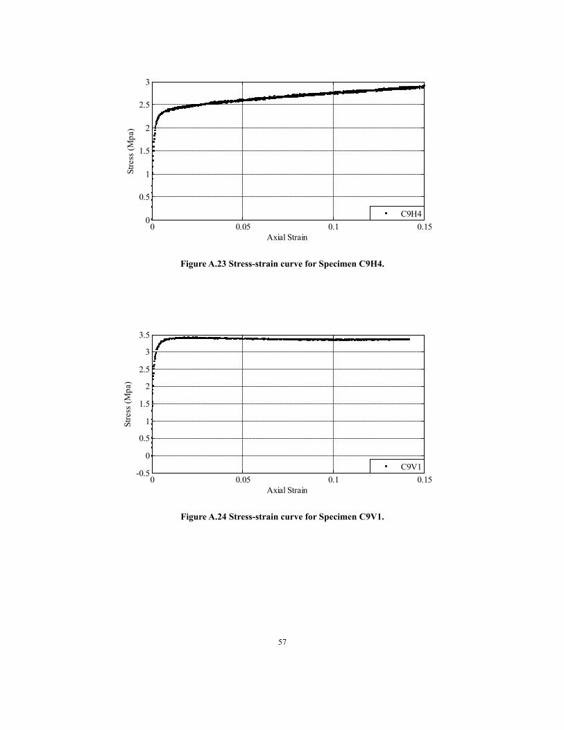
57



0 0.05 0.1 0.150

0.5

1

1.5

2

2.5

3

Axial Strain

Stre

ss (M

pa)

C9H4

0 0.05 0.1 0.15-0.5

0

0.5

1

1.5

2

2.5

3

3.5

Axial Strain

Stre

ss (M

pa)

C9V1

58



0 0.05 0.1 0.150

1

2

3

4

5

6

Axial Strain

Stre

ss (M

pa)

C9V2

0 0.05 0.1 0.150

1

2

3

4

Axial Strain

Stre

ss (M

pa)

C9V3

59



0 0.05 0.1 0.150

0.5

1

1.5

2

2.5

3

3.5

Axial Strain

Stre

ss (M

pa)

C9V4

0 0.05 0.1 0.15-0.5

0

0.5

1

1.5

2

2.5

3

Axial Strain

Stre

ss (M

pa)

C9V5

60



0 0.05 0.1 0.15-1

0

1

2

3

4

5

6

Axial Strain

Stre

ss (M

pa)

C9V6

0 0.05 0.1 0.150

1

2

3

4

5

Axial Strain

Stre

ss (M

pa)

C10H1

61



0 0.05 0.1 0.150

0.5

1

1.5

2

2.5

3

3.5

Axial Strain

Stre

ss (M

pa)

C10H2

0 0.05 0.1 0.150

1

2

3

4

5

Axial Strain

Stre

ss (M

pa)

C10H3

62



0 0.05 0.1 0.150

1

2

3

4

5

Axial Strain

Stre

ss (M

pa)

C10H4

0 0.05 0.1 0.150

1

2

3

4

5

6

Axial Strain

Stre

ss (M

pa)

C10H6

63



0 0.05 0.1 0.150

1

2

3

4

5

Axial Strain

Stre

ss (M

pa)

C10V1

0 0.05 0.1 0.150

1

2

3

4

5

6

Axial Strain

Stre

ss (M

pa)

C11V1

64



0 0.05 0.1 0.150

2

4

6

8

Axial Strain

Stre

ss (M

pa)

C11V2

0 0.05 0.1 0.15-1

0

1

2

3

4

5

Axial Strain

Stre

ss (M

pa)

C11V4

65

Figure A.39 Stress-strain curve for Specimen P4H1.


0 0.05 0.1 0.150

0.5

1

1.5

2

2.5

3

3.5

Axial Strain

Stre

ss (M

pa)

P4H1

0 0.05 0.1 0.150

0.5

1

1.5

2

2.5

Axial Strain

Stre

ss (M

pa)

P4H4

66

Figure A.41 Stress-strain curve for Specimen P4V1.


0 0.05 0.1 0.150

1

2

3

4

Axial Strain

Stre

ss (M

pa)

P4V1

0 0.05 0.1 0.150

0.5

1

1.5

2

2.5

3

Axial Strain

Stre

ss (M

pa)

P4V2

67



0 0.05 0.1 0.150

0.5

1

1.5

2

2.5

Axial Strain

Stre

ss (M

pa)

P4V3

0 0.05 0.1 0.150

0.5

1

1.5

2

2.5

Axial Strain

Stre

ss (M

pa)

P4V4

68



0 0.05 0.1 0.150

1

2

3

4

5

6

Axial Strain

Stre

ss (M

pa)

P6H1

0 0.05 0.1 0.150

1

2

3

4

5

6

Axial Strain

Stre

ss (M

pa)

P6H2

69



0 0.05 0.1 0.150

1

2

3

4

5

Axial Strain

Stre

ss (M

pa)

P6H3

0 0.05 0.1 0.150

0.5

1

1.5

2

2.5

3

3.5

Axial Strain

Stre

ss (M

pa)

P6V1

70



0 0.05 0.1 0.150

0.5

1

1.5

2

2.5

3

3.5

Axial Strain

Stre

ss (M

pa)

P6V2

0 0.05 0.1 0.150

1

2

3

4

5

6

7

Axial Strain

Stre

ss (M

pa)

P8H1

71



0 0.05 0.1 0.150

1

2

3

4

5

6

7

Axial Strain

Stre

ss (M

pa)

P8H2

0 0.05 0.1 0.150

0.5

1

1.5

2

2.5

3

Axial Strain

Stre

ss (M

pa)

P8V1

72



0 0.05 0.1 0.150

0.5

1

1.5

2

2.5

3

3.5

Axial Strain

Stre

ss (M

pa)

P8V2

0 0.05 0.1 0.150

1

2

3

4

5

6

Axial Strain

Stre

ss (M

pa)

P9H1

73



0 0.05 0.1 0.150

1

2

3

4

5

6

7

Axial Strain

Stre

ss (M

pa)

P9H2

0 0.05 0.1 0.150

1

2

3

4

Axial Strain

Stre

ss (M

pa)

P9V1

74



0 0.05 0.1 0.15-1

0

1

2

3

4

5

Axial Strain

Stre

ss (M

pa)

P9V4

0 0.05 0.1 0.15-1

0

1

2

3

4

Axial Strain

Stre

ss (M

pa)

P11V1

75



0 0.05 0.1 0.150

1

2

3

4

5

Axial Strain

Stre

ss (M

pa)

P11V2

0 0.05 0.1 0.15-1

0

1

2

3

4

Axial Strain

Stre

ss (M

pa)

P11V3

Documents

Frozen Soil Lateral Resistance for the Seismic Design of