Full 3D Dispersion Curve Solutions for Guided Waves in

Generally Anisotropic Media0

F. Hernando Quintanillaa, M. J. S. Lowea and R. V. Crasterb

aDepartment of Mechanical Engineering, bDepartment of Mathematics, Imperial College,London SW7 2AZ, UK

Abstract

Dispersion curves of guided waves provide valuable information about thephysical and elastic properties of waves propagating within a given waveguidestructure. Algorithms to accurately compute these curves are an essentialtool for engineers working in non-destructive evaluation and for scientistsstudying wave phenomena. Dispersion curves are typically computed for lowor zero attenuation and presented in two or three dimensional plots. Theformer do not always provide a clear and complete picture of the dispersionloci and the latter are very difficult to obtain when high values of attenuationare involved and arbitrary anisotropy is considered in single or multi-layeredsystems. As a consequence, drawing correct and reliable conclusions is achallenging task in the modern applications that often utilise multi-layeredanisotropic viscoelastic materials. These challenges are overcome here by us-ing a spectral collocation method (SCM) to robustly find dispersion curvesin the most complicated cases of high attenuation and arbitrary anisotropy.Solutions are then plotted in three-dimensional frequency-complex wavenum-ber space, thus gaining much deeper insight into the nature of these prob-lems. The cases studied range from classical examples, which validate thisapproach, to new ones involving materials up to the most general triclinicclass for both flat and cylindrical geometry in multi-layered systems. Theapparent crossing of modes within the same symmetry family in viscoelasticmedia is also explained and clarified by the results. Finally, the consequencesof the centre of symmetry, present in every crystal class, on the solutions arediscussed.

0Accepted for publication in the Journal of Sound and Vibration,

Preprint submitted to Elsevier November 18, 2015

1. Introduction

In the study, and engineering application, of elastic guided waves the dis-persion curves of waves propagating within a given structure are a vital toolfor inspection purposes and for obtaining information about the properties ofthe material itself. Dispersion curves for propagating and non-propagatingmodes are often computed for zero, or low, attenuation values and presentedas two or three dimensional plots. See for instance [1], [2], [3] or more re-cently [4], [5] and [6]. However, cases where high values of attenuation arepresent and arbitrary anisotropy in single or multi-layered structures is con-sidered have been hardly studied due to the great difficulties encounteredwhen computing their dispersion curves. For instance, dispersion curves forviscoelastic monoclinic plates have been found and, for low values of the at-tenuation, presented in two dimensional plots [7], but in general, a betterunderstanding of the nature of the modes, and a clearer visualization of thesolutions, is achieved when dispersion loci are reliably found for low as wellas high values of attenuation and therefore dispersion curves are required inthree dimensions.

In the literature, modes have been categorised in a number of ways and herethe classification of Auld [8] is used: propagating modes have real wavenum-ber, for this reason they are often the most useful for engineering applicationin NDT since they propagate and transport energy within the structure with-out attenuation. The second type of solution is non-propagating modes withcomplex or purely imaginary wavenumber. Note that these modes with com-plex or purely imaginary wavenumbers are also present in perfectly elasticmaterials without any energy leakage, those solutions represent local modesthat would exist at discontinuities. In addition, non-propagating modes areof interest in certain applications such as the solution of scattering problemsusing modal summations where a knowledge of the full set of possible modesis essential, [9]. A detailed discussion about the physical properties and en-ergy transportation of non-propagating modes in elastic (lossless) media is inthe second volume of Auld [8]. For viscoelastic materials, only propagatingmodes with complex wavenumber exist lest unphysical results are obtainedas pointed out in [6]. Propagating modes in viscoelastic media can in turnbe split into: lowly attenuated modes, with almost real wavenumbers and

DOI:10.1016/j.jsv.2015.10.017, November 2015.

2

therefore very useful for inspection purposes in NDT; and highly attenuatedmodes, with dominant imaginary part for the wavenumbers. The reader mustbe aware that there does not seem to be a consensus about this nomenclature,see for example [8], [10] and [11]. In this paper we adopt the convention byAuld [8] and we will try to make it clear what kind of modes we are talkingabout in each case by specifying the nature of the wavenumber. Collectively,these types of modes constitute the complete spectrum for a given problemand their study and visualization is the object of our current investigation.

Several methods have been developed, and successfully deployed, to com-pute two-dimensional, and less often three-dimensional, dispersion curves forguided waves in flat and cylindrical geometry: finite element (FE), semi-analytical finite element (SAFE) simulations, root-finding routines based onthe partial wave approach (Partial Wave Root Finding, PWRF) and lately,spectral methods have become more popular as a powerful alternative, see[4], [12] or [13]. More recently, one of these variants known as Spectral Col-location Method (SCM) has been successfully used to model guided waves inelastic and viscoelastic generally anisotropic media, [14] and [15] respectively.

The main contribution and novelty of the present paper is the deploymentof a SCM to compute the full three-dimensional spectrum, including highlyattenuated and non-propagating purely imaginary modes, for guided waveproblems in three cases (Figures 4.a, 5.a, 7 and 9.) which, to the best of theauthors’ knowledge, have not been studied before and comprise up to themost general type of anisotropy, namely triclinic crystals. Several other well-known cases have also been presented for validation purposes. Regardless ofthe case under study, this investigation also emphasizes that with the SCM noadditional coding effort is needed to obtain the complete three-dimensionalspectrum which contrasts with conventional approaches for which the al-gorithms become significantly more inefficient when searching in a three-dimensional space and which may require substantial modification to obtainrobust solutions. The SCM used here was first presented in a previous workby Hernando et. al [15], though there, attention was restricted solely to lowlyattenuated modes. The present work goes one step further and, by carefullysorting the eigenvalues provided by the SCM, completes the picture givingthe remaining branches of the dispersion loci for the most general anisotropictriclinic class. It is notable that with technological advances there is a needfor this full anisotropic generality and for the robust generation of the corre-

3

sponding three-dimensional dispersion curves presented in this paper for thefirst time.

Additional contributions of this paper, arising from the undertaken inves-tigations, are the clarifications concerning the apparent crossing of modeswithin the same symmetry family for viscoelastic media (Section III) andthe discussion of the implications of the centre of symmetry of all crystalclasses for the solution (Section V).

The paper is organized as follows. In section 2 a very brief description ofthe SCM, and its implementation is given, this is kept to a minimum toavoid repetition and the reader is referred to [12], [14], [15] and referencestherein for all the details about the SCM scheme and an extensive discussionof its principal features when used to solve acoustic guided wave problems.Some modifications are required here and these are outlined. In section 3,classical examples in flat geometry both for elastic and viscoelastic mediaare presented as a further validation of the SCM approach. The crossing ofmodes, which is an important detail in practice, is discussed and elucidatedwith the aid of a new three-dimensional plot for the dispersion curves of amonoclinic material. The full solution for a new multilayer flat case is pre-sented at the end of section 3. Section 4 treats cylindrical geometry, firstlya classical example is briefly presented for validation and the section closeswith a new illustrative multilayer cylindrical system. Section 5 is devoted tothe discussion of the results and conclusions.

2. SCM methodology outline

A comprehensive description of the SCM is in [12], [14] and, with partic-ular relevance to the present case, in [15]. The main idea behind the SCMis to convert the partial differential equations of the acoustic field into ageneralized matrix eigenvalue problem whose eigenvalues are computed thusyielding the full spectrum. We highlight some minor modifications regardingthe post processing of results which must be done in order to visualize thefull three-dimensional solution.

The governing equations of motion for a linear elastic anisotropic homo-geneous medium are:

∇iKcKL∇symLj uj = −ρ ω2 ui (1)

4

with the summation convention over the indices and cKL is the medium’sstiffness matrix in reduced index notation, [8] , uj are the components of thedisplacement vector field that for the application here are

uj = Uj(y) ei(kz−ωt) ; j = x, y, z. (2)

The differential operators in (1) are of first order in the coordinate derivativesand their explicit expressions are in [8]. The expression of the stress tensorfield in terms of the strain tensor field, Skl, for a perfectly elastic materialreads:

Tij = cijkl Skl (3)

here cijkl is the fourth-rank stiffness tensor related to cKL as described in[8]. When material damping is included, that is, when modelling viscoelasticmedia, the viscoelastic stress tensor field takes the following more complexform assuming the Kelvin-Voigt frequency dependent model (see [15] fordetails) to account for material damping:

cKVpjkl = cpjkl − i

ω

ωηpjkl (4)

Where cpjkl and ηpjkl have the same units and the prefactor ω/ω is non-dimensional. The ηpjkl tensor accounts for losses within the material. Amore detailed description of the derivation of this expression is in Auld [8].For structures in a vacuum, traction-free boundary conditions hold. Theserequire the vanishing of the following three components of the stress tensorfield. Taking the faces of the plate to be located at y = ±h/2 the boundaryconditions (BCs) are given by:

Tyy|y=±h/2 = Tyx|y=±h/2 = Tyz|y=±h/2 = 0. (5)

Turning now to the implementation of the SCM, the standard procedureconsists of discretizing the physical domain and replacing the derivatives inEq. (1) by the discrete Differentiation Matrices (DMs). For a single layer invacuum, since we have a bounded interval, an appropriate, spectrally accu-rate, choice is to use Chebyshev DMs, based on a non-uniform Chebyshevgrid of N points, these are N×N matrices; the generation of DMs is covered

5

in [16], [17]. The m-th derivative with respect to y is approximated by thecorresponding m-th order Chebyshev N ×N DM:

∂(m)

∂y(m)=⇒ D(m) := [DMCheb]

(m)N×N (6)

The substitution is made in both the equations of motion Eq. (1) and bound-ary conditions Eq. (5) yielding the matrix analogue that is concisely writtenas:

L(k) U = ω2 M U (7)

where U is the vector of vectors : U = [Ux,Uy,Uz]T , these vectors Ui are

the components of the displacement vector field. The matrix L(k) containsthe differential operators of the PDEs and the matrix M is the identity mul-tiplied by −ρ. The boundary conditions (BC) in Eq. (5) are taken intoaccount by appropriately substituting them in the corresponding rows of Eq.(7) after having recast them in matrix form, in the same fashion as was donefor the equations of motion, this procedure is described in detail in [14].

The L(k) matrix contains terms proportional to k0, k1 and k2. Rearrangingthe terms in the matrix equation Eq. (7) and decomposing the L(k) matrixso that the k dependence of the different terms becomes more apparent leadsto the following expression of Eq. (7):(

Q2 k2 + Q1 k + Q0(ω

2))U = 0 (8)

Now it should be clear that, once we fix the value of ω, this does not havethe structure of a general eigenvalue problem in k. In order to achieve thisstructure (see Eq. (7)), a mathematical technique known as the Linear Com-panion Matrix Method is used, see [18], [19] or [15]. Once we recast this againin the form of Eq. (7) which is a typical generalized eigenvalue problem, it iseasily solved using an eigensolver routine that yields the complex eigenvaluesk ; the cases presented here were solved with the routine eig of MATLAB(version R2012b).

The SCM is known to produce some spurious eigenvalues as pointed outin [20] and [12] for instance. The methodologies to deal with them havebeen extensively discussed there and a similar discussion will not be pursuedhere. These general procedures apply equally in the present case but in vis-coelastic materials the full solution comprises all possible modes described

6

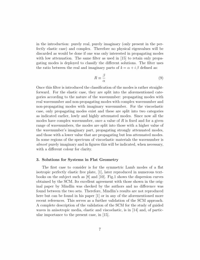
in the introduction: purely real, purely imaginary (only present in the per-fectly elastic case) and complex. Therefore no physical eigenvalues will bediscarded as would be done if one was only interested in propagating modeswith low attenuation. The same filter as used in [15] to retain only propa-gating modes is deployed to classify the different solutions. The filter usesthe ratio between the real and imaginary parts of k = α + i β defined as:

R ≡ β

α(9)

Once this filter is introduced the classification of the modes is rather straight-forward. For the elastic case, they are split into the aforementioned cate-gories according to the nature of the wavenumber: propagating modes withreal wavenumber and non-propagating modes with complex wavenumber andnon-propagating modes with imaginary wavenumber. For the viscoelasticcase, only propagating modes exist and these are split into two categoriesas indicated earlier, lowly and highly attenuated modes. Since now all themodes have complex wavenumber, once a value of R is fixed and for a givenrange of wavenumbers, the modes are split into those with a higher value ofthe wavenumber’s imaginary part, propagating strongly attenuated modes,and those with a lower value that are propagating but less attenuated modes.In some regions of the spectrum of viscoelastic materials the wavenumber isalmost purely imaginary and in figures this will be indicated, when necessary,with a different colour for clarity.

3. Solutions for Systems in Flat Geometry

The first case to consider is for the symmetric Lamb modes of a flatisotropic perfectly elastic free plate, [1], later reproduced in numerous text-books on the subject such as [8] and [10]. Fig.1 shows the dispersion curvesobtained by the SCM. Its excellent agreement with those shown in the orig-inal paper by Mindlin was checked by the authors and no difference wasfound between the two sets. Therefore, Mindlin’s results are not reproducedhere but can be found in his paper [1] or in any of the aforementioned morerecent references. This serves as a further validation of the SCM approach.A complete description of the validation of the SCM for the study of guidedwaves in anisotropic media, elastic and viscoelastic, is in [14] and, of partic-ular importance to the present case, in [15].

7

Figure 1: First three symmetric Lamb modes in a free elastic steel plate computed withthe SCM. Propagating modes (lowly attenuated modes) in blue. Non-propagating highlyattenuated modes in red and black (purely imaginary). The non-dimensional axes are Ω= hω / πV66 and Ψ = hk / π.

8

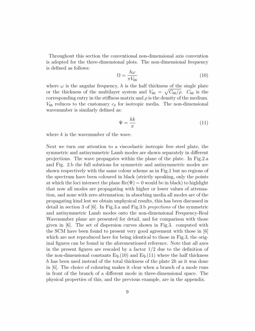
Throughout this section the conventional non-dimensional axis conventionis adopted for the three-dimensional plots. The non-dimensional frequencyis defined as follows:

Ω =hω

πV66(10)

where ω is the angular frequency, h is the half thickness of the single plateor the thickness of the multilayer system and V66 =

√C66/ρ. C66 is the

corresponding entry in the stiffness matrix and ρ is the density of the medium.V66 reduces to the customary c2 for isotropic media. The non-dimensionalwavenumber is similarly defined as:

Ψ =hk

π(11)

where k is the wavenumber of the wave.

Next we turn our attention to a viscoelastic isotropic free steel plate, thesymmetric and antisymmetric Lamb modes are shown separately in differentprojections. The wave propagates within the plane of the plate. In Fig.2.aand Fig. 2.b the full solutions for symmetric and antisymmetric modes areshown respectively with the same colour scheme as in Fig.1 but no regions ofthe spectrum have been coloured in black (strictly speaking, only the pointsat which the loci intersect the plane Re(Ψ) = 0 would be in black) to highlightthat now all modes are propagating with higher or lower values of attenua-tion, and none with zero attenuation; in absorbing media all modes are of thepropagating kind lest we obtain unphysical results, this has been discussed indetail in section 3 of [6]. In Fig.3.a and Fig.3.b projections of the symmetricand antisymmetric Lamb modes onto the non-dimensional Frequency-RealWavenumber plane are presented for detail, and for comparison with thosegiven in [6]. The set of dispersion curves shown in Fig.3. computed withthe SCM have been found to present very good agreement with those in [6]which are not reproduced here for being identical to those in Fig.3, the orig-inal figures can be found in the aforementioned reference. Note that all axesin the present figures are rescaled by a factor 1/2 due to the definition ofthe non-dimensional constants Eq.(10) and Eq.(11) where the half thicknessh has been used instead of the total thickness of the plate 2h as it was donein [6]. The choice of colouring makes it clear when a branch of a mode runsin front of the branch of a different mode in three-dimensional space. Thephysical properties of this, and the previous example, are in the appendix.

9

Figure 2: Symmetric (a) and Antisymmetric (b) Lamb modes in a free hysteretic-typeviscoelastic steel plate computed with the SCM. Propagating modes in blue (lowly atten-uated) and red (highly attenuated). Non-dimensional axes: Ω = hω / πV66 and Ψ = hk/ π.

It is important to note already that the apparent crossing of modes withinthe same family, something forbidden in the elastic case, does not actuallytake place in the viscoelastic case either. This is explained by noticing thatfor the viscoelastic case one still has two independent dispersion relations forLamb modes whose entries are now complex, thus yielding generally complexroots: See also Rose [11] or Graff [10] for a more detailed discussion aboutthis. The splitting of modes into families of symmetric and antisymmetricLamb modes is related to the geometrical symmetries of the crystal and axesconfiguration for the crystal chosen in each case, not to the dynamical prop-erties of the material itself such as damping. Therefore, regardless of thematerial being elastic or viscoelastic, if the crystal configuration is such thatmodes can be classified according to their symmetry with respect to the mid-dle plane of the plate, those two families will remain independent from eachother for any kind of media and no crossing between them will occur. Thisis seen by looking at the full 3D picture of the dispersion curves and noting

10

Figure 3: 2D projection of the symmetric (a) and antisymmetric (b) Lamb modes in afree hysteretic-type viscoelastic steel plate computed with the SCM shown in figure 2.Propagating modes in blue (lowly attenuated) and red (highly attenuated).

that what seems to be a crossing in the 2D projection is nothing more thanone line passing in front of the other in the complete and clearer 3D picture.This is a recurrent point of discussion in the literature, to cite only a few,see for instance [21], [22] and [23], it has also been addressed in [6] and in [5]for elastic plates with fluid loading, further references to other related paperscan be found therein. The next example will further verify this assertion inthe case of a more complex material.

Now a free viscoelastic plate of monoclinic material is investigated. Thecrystal configuration is as follows: the Y axis of the crystal is normalto the plane of the plate and propagation takes place along the Z axis,further details about the physical properties of the material are in the ap-pendix. Fig. 4.a and Fig. 5.a present the full three-dimensional solution forsymmetric and antisymmetric coupled modes respectively in a monoclinicplate which, to the best of the author’s knowledge, has not been presentedbefore. Its corresponding two-dimensional plots for propagating modes andattenuation are shown in Fig.4.b and Fig.4.c for symmetric modes and inFig.5.b and Fig.5.c for antisymmetric modes respectively. It is shown in Fig.

11

4.b that two of the symmetric modes, labelled as B and C, cross at roughly0.50 MHz, a similar result was obtained and discussed in figure 5 of [7] fora different monoclinic plate. Note that the modes labelled A and B do notcross. Once more, it is worth emphasizing that no real crossing occurs in thiscase for the same reasons mentioned in the previous paragraph. For instance,Li and Thompson [24] derived the two generalized Lamb dispersion relationsfor symmetric and antisymmetric modes in a monoclinic plate with propa-gation within the plane of symmetry of the crystal, these were also derivedin [25].

These two independent dispersion relations derived in [24] hold also for thecase of viscoelastic materials and therefore, having only one dispersion re-lation which cannot be further factorized into a simpler product of factorsfor each independent family, no crossings can occur amongst modes given bythe corresponding non-reducible dispersion relation for the independent fam-ily under study. The fact that these dispersion relations cannot be furtherfactorized has a physical interpretation as explained by Solie and Auld [26]:each dispersion relation is the determinant of the coefficient matrix of a set ofequations whose unknowns are the amplitudes of the partial waves which giverise to the family of modes considered and the order of this non-reducibledeterminant is equal to the minimum number of partial waves needed forsatisfying the boundary conditions. The six partial waves will be coupledby the boundary conditions and anisotropy of the crystal in various wayswhich depend on the problem under study. Note that the partial waves arementioned here because they are a known valid means of representing theguided wave fields, and are thus a useful tool to aid the explanation, but itmust be emphasised that partial waves are not part of the alternative SCMapproach presented in this work. In the present case, three partial waves arecoupled (coupling symmetric SH and Lamb modes) to give rise to the coupledsymmetric modes, analogously for antisymmetric modes. Similar consider-ations and explicit formulae for the monoclinic case can be found also in [27].

The assertion that no crossings occur and the solution given by each ofthese non-reducible dispersion relations is unique can be explained as follows:Firstly, the non-reducibility of an N×N dispersion determinant implies thatone needs at least as many partial waves as the order of the determinant tosatisfy the boundary conditions, that is, N . Secondly, in order to have non-trivial solutions one requires the N × N determinant to vanish, this means

12

Figure 4: Top: Symmetric generalized Lamb modes in a free hysteretic-type viscoelasticmonoclinic plate computed with the SCM (a). Propagation is along the Z axis, and theY axis is perpendicular to the plane of the plate. Propagating Modes: low attenuatedmodes in blue, highly attenuated modes in red and almost imaginary wavenumber modesin black. Plot non-dimensional axes: Ω = hω / πV66 and Ψ = hk / π. Bottom: 2Ddispersion curves (b) and attenuation (c) of the symmetric generalized Lamb modes inthe viscoelastic monoclinic plate. Note the apparent crossing of modes B and C in (b) atroughly 0.5 MHz.

13

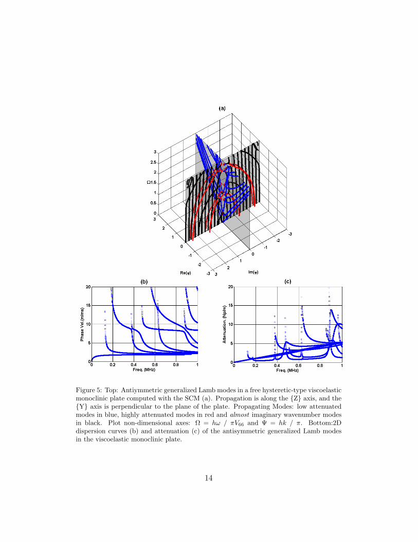
Figure 5: Top: Antiymmetric generalized Lamb modes in a free hysteretic-type viscoelasticmonoclinic plate computed with the SCM (a). Propagation is along the Z axis, and theY axis is perpendicular to the plane of the plate. Propagating Modes: low attenuatedmodes in blue, highly attenuated modes in red and almost imaginary wavenumber modesin black. Plot non-dimensional axes: Ω = hω / πV66 and Ψ = hk / π. Bottom:2Ddispersion curves (b) and attenuation (c) of the antisymmetric generalized Lamb modesin the viscoelastic monoclinic plate.

14

the rank of the determinant is no bigger than (N − 1).

It can be seen that the rank is in fact (N − 1) thus yielding a unique non-trivial solution by the following consideration: if this was not so, and letus assume for definiteness that it was (N − 2), one could find non-trivialsolutions expressing (N − 2) partial wave amplitudes in terms of the tworemaining ones. In particular, one could set one of these latter amplitudes tozero while still having a non-trivial solution constructed from (N −1) partialwaves. This is in stark contradiction with the need for at least N partialwaves implied by the non-reducibility of the N ×N dispersion determinant.

Interestingly, this can be confirmed by the SCM which uses an algebraicapproach. It has been observed that for each independent family of modesthe multiplicity of the eigenvalues, roots of the dispersion relation, is one.This means that the eigenspace spanned by the corresponding eigenvector(mode) is one-dimensional, which is tantamount to saying that only one dis-persion curve runs through that point. Moreover, when a code for the mostgeneral case of triclinic is used to study the dispersion curves in an isotropicplate, the four independent families of modes (Symmetric/AntisymmetricLamb and SH) are obtained and, up to the accuracy allowed by computerprecision, it can be seen that eigenvalues with multiplicity two are obtainedfor the crossing points. Their two eigenvectors are orthogonal which meansthere are two different modes for that given eigenvalue: for instance an SHand a Lamb mode. In Fig.6, a detail of the problematic region in Fig.4.baround 0.50 MHz is presented in three-dimensional space and it is seen veryclearly that these two modes do not cross.

Finally for flat geometry we consider a bilayered system composed of a vis-coelastic triclinic plate and an elastic orthorhombic plate. Figure 7 showsits three-dimensional complete spectrum which, to the best of the author’sknowledge, has not yet been published for this or similar systems involv-ing crystals of triclinic symmetry. The axis configuration is the same as inthe previous example: the Y axis of the crystal is normal to the plane ofthe plates and the propagation takes place along the Z axis. More de-tails about the physical properties of the plates are given in the appendix.This highlights the usefulness of the SCM approach for calculating the fullspectrum of complicated cases of single or even multi-layered systems withdifferent viscoelastic materials or combinations of elastic/viscoelastic mate-

15

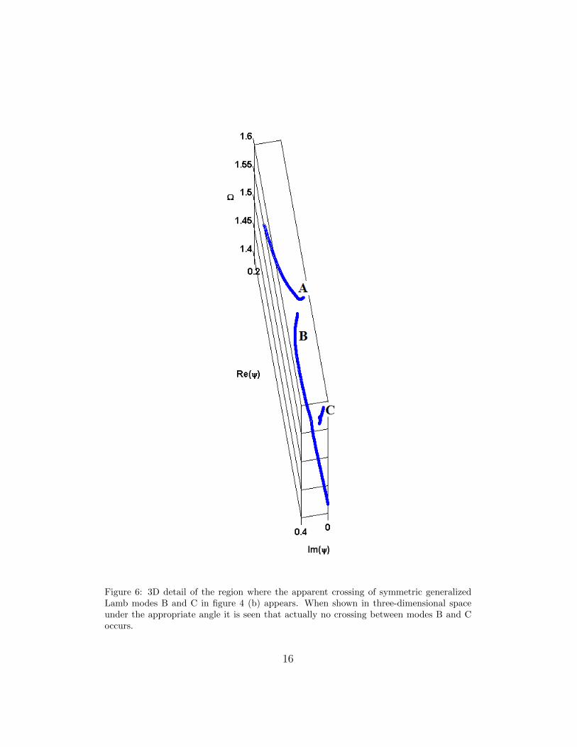
Figure 6: 3D detail of the region where the apparent crossing of symmetric generalizedLamb modes B and C in figure 4 (b) appears. When shown in three-dimensional spaceunder the appropriate angle it is seen that actually no crossing between modes B and Coccurs.

16

rials. Similar solutions for much simpler systems are sometimes incompletewhen they are computed by conventional root-finding routines for instance,which highlights the importance of the methodology and results shown inthe present work. As a consequence of this, some of the modes might alsoappear to merge with each other. These difficulties are easily overcome byusing a SCM that provides, without any extra coding effort, the full three-dimensional solution; a detailed discussion of further advantages of the SCMfor guided wave problems is given in [12], [14] or [15]. The choice of mate-rials, in particular the triclinic layer, has been done in order to provide thesolution for as general a case as possible, thus a triclinic layer has been in-cluded. Note that in the work by Hernando et. al [15] only the conventionaltwo dimensional dispersion curves for lowly attenuated modes was presentedthough not a complete solution as the one given here.

4. Solutions for Systems in Cylindrical Geometry

Only two examples are shown in this section since the procedure to ob-tain the full solution in cylindrical geometry follows exactly the same linesas that for flat plates. In addition, a detailed study of these systems for non-attenuating and low-attenuating modes has been already carried out in [15].Therefore, a classical example from the literature and a sufficiently generalnew case suffices to illustrate the capabilities of the SCM when obtaining fullsolutions in cylindrical geometry.

Throughout this section for cylindrical geometry, the conventional non-dimensionalaxes convention is adopted for the three-dimensional plots. The non-dimensionalfrequency is defined as follows:

Ω =aω

V66(12)

where ω is the angular frequency, a is the thickness of the cylindrical shellsystem or the radius of the rod and V66 =

√C66/ρ. C66 is the corresponding

entry in the stiffness matrix and ρ is the density of the medium. V66 reducesto the customary c2 for isotropic media. The non-dimensional wavenumberis similarly defined as:

Ψ = ak (13)

where k is the wavenumber of the wave.

17

Figure 7: Modes in a free bilayer plate system: 5 mm thick elastic orthorhombic plate and 3mm hysteretic-type viscoelastic triclinic plate computed with the SCM. Propagation alongthe Z axis and the Y axis perpendicular to the plane of the plate. Propagating Modes:low attenuated modes in blue, highly attenuated modes in red and almost imaginarywavenumber modes in black. Plot non-dimensional axes: Ω = hω / πV66 and Ψ = hk / π.

18

Figure 8: Flexural n=1 modes in free elastic steel rod with radius r = 20 mm. Thisagrees well with the corresponding 2D plot first published by Pao [28]. Wave propagationalong the z axis of the cylinder. Propagating modes (lowly attenuated modes) in blue.Non-propagating highly attenuated modes in red and black (purely imaginary). Plot non-dimensional axes: Ω = aω / V66 and Ψ = ak.

The first example shows the dispersion curves for flexural modes with har-monic order n = 1 in an elastic cylindrical steel rod where the propagationtakes place along the axis of the cylinder. Fig.8 shows the spectrum computedby the SCM which were compared by the authors to the two-dimensional plotin Pao [28] showing excellent agreement. The original figure by Pao has notbeen included in this paper in order to avoid repetititon of identical figuresbut the reader can easily find it in the reference provided. As pointed outin the literature [10], it can be seen in Fig.8 that the incomplete imagi-nary black branches (non-propagating purely imaginary modes) are linked inthree-dimensional space by complex red branches (non-propagating modeswith complex wavenumber). Further details about the physical and geomet-rical properties are in the appendix.

To close this section a final new case is presented. Flexural n = 0 modes

19

(Longitudinal coupled with Torsional) in a hollow cylinder composed of twodifferent layers are studied with propagation along the axis of the cylinder.The innermost layer is a triclinic viscoelastic plate of thickness ho = 3 mmand the outer layer is an elastic orthorhombic plate of thickness hi = 5 mmwhose fibres along the z axis have been rotated 45 degrees to form anhelicoidal path around the cylinder’s axis, the internal radius of the cylinderis ri = 17 mm. The three-dimensional spectrum computed by the SCM isshown in Fig.9 for the first five modes; two-dimensional dispersion curves forthe propagating modes have already been shown in the literature for similarsystems, see [15], but the full spectrum for anisotropic materials presentedhere has not been published elsewhere to the best of the authors’ knowledge.Due to the presence of an absorbing layer, all modes are propagating: withvery low attenuation showing in blue, with highly attenuated modes show-ing in red and modes with almost imaginary wavenumber showing in black.Note that, strictly speaking, these latter modes should have been colouredin red too. However, since the system contains a perfectly elastic layer somebranches show a behaviour closer to that featured in the perfectly elastic caseand thus have a very small real part, though not strictly zero. In order tomake this more apparent and clear, the authors have chosen to colour themin black for this figure. Again, the triclinic layer has been chosen because ofits generality, thus showing that the SCM can provide the complete three-dimensional spectrum for the most general cases in cylindrical geometry. Itis notable that with advances in technology it is these complicated multilayerand generally anisotropic cases that now require modelling.

5. Discussion of Results and Conclusions

The capability of the SCM approach to find full three-dimensional so-lutions for dispersion curves has been demonstrated here. The SCM hascomputed the complete spectrum of various known cases, as well as somenew settings, efficiently and accurately, without modifying the algorithm, tofind all the eigenvalues. This advantage of not missing any modes has beenrepeatedly emphasized in the literature in other contexts ([16] or [20]) andin previous papers on guided waves ([12], [14] or [15]), the interested readercan find a detailed discussion about this and other advantages of the SCMin those references.

The SCM throws new light onto problems involving elastic or viscoelastic

20

Figure 9: Flexural n=0 modes in free two-layered cylinder. The inner layer is a kelvin-voigt-type viscoelastic triclinic crystal of thickness hi = 5 mm and the outer layer isan elastic orthorhombic crystal of thickness ho = 3 mm whose fibres along the z axishave been rotated 45 degrees to form an helicoidal path around the cylinder’s axis. Thecylinder’s inner radius is ri = 17 mm. Propagation along the z axis of the cylinder.Propagating Modes: low attenuated modes in blue, highly attenuated modes in red andalmost imaginary wavenumber modes in black. Plot non-dimensional axes: Ω = aω / V66and Ψ = ak.

media which are often very demanding for conventional approaches (root-finding routines or FE simulations), for instance, for a two-layer system ofisotropic and orthorhombic viscoelastic materials. For those cases where theroot-finding routines work, one often finds that the solutions are incompleteand the path of the dispersion curves is unclear thus giving the impression ofmode merging and similar unusual phenomena. This troublesome situationcan sometimes be elucidated by tedious work refining the search algorithmto complete the missing parts in a three-dimensional space and get the fullpicture of the spectrum. FE simulations are a good and useful alternativeto root-finding routines and can also model any material and configuration.However, FE simulations require a far greater coding effort, understanding

21

of the methodology and a careful examination of the solutions to discardthe spurious unphysical modes; a more detailed discussion about this is in[15]. It is seen that the SCM yields the complete solution straightforwardly;only an adequate post processing of the results is needed to clearly plot thedifferent parts of the spectrum according to the nature of the wavenumber.

In addition to the classical examples from the literature, the SCM has suc-cessfully computed the complete three-dimensional spectrum of the mostgeneral and complicated cases which, to the best of the authors’ knowledge,had not been presented before. Even though similar general cases have beensolved recently by Hernando et. al [14] for perfectly elastic media and byHernando, Fan et. al for viscoelastic materials [15], they focus solely onlowly attenuated modes and their corresponding two-dimensional dispersioncurves. Therefore, it is hoped that the investigations presented here con-tribute to complete the picture in the most general and until now unknowncases.

The general examples involving triclinic materials presented earlier have high-lighted the need of a clarification regarding the symmetries of crystals andthe consequences on the waves propagating within them. In the literature,the symmetry properties of the Lamb dispersion equations are often used forsimplification or to draw certain conclusions about the nature of the solution.For instance in [4] they take advantage of the symmetry k ↔ −k to reducethe dimension of the matrix. Another example of this assertion can be foundin Graff [10] (chapter 8, page 455). From this, one might draw the erroneousconclusion that when the dispersion relation lacks that symmetry, so willits solutions. Triclinic materials’ dispersion relation, for instance, lack thissymmetry as shown in [25]. In the course of the present investigation onecan see that in spite of the absence of this symmetry in triclinic materials, itssolution shows this k ↔ −k symmetry. This apparent paradox is solved bynoticing that the mentioned symmetry has a deeper source than the formalstructure of the dispersion relation: all crystal classes possess one centre ofsymmetry, see for example [29], which means that they are invariant underthe change ~r ↔ −~r, which in general is not the same as a mirror symmetrythrough the plane normal to the direction of the wave vector. Therefore, re-gardless of the formal structure of the dispersion relation, every crystal willdisplay that intrinsic symmetry as the examples in the present work reveal.

22

Apart from the observation made in the previous paragraph, it has alsobeen pointed out and explained at the end of section III why the modes ofthe same symmetry family in a free viscoelastic plate do not cross. Thisapparent crossing is merely a visual effect of the projection of the dispersionloci onto a two-dimensional plane which is readily clarified when one looksat the full three-dimensional solution and realizes that for each independentfamily there is only one dispersion relation, the very same as in the elasticcase, which cannot be further factorized. It is also important to notice thefollowing: one might argue that the example presented in Fig.1 is actually aperfect counterexample for the statement given in section III, namely, thathaving only one dispersion relation which cannot be further factorized foreach family, no crossings can occur amongst modes within the same fam-ily. Careful consideration shows that this is not the case. As explained byAuld [8] (Chapter 10, Volume II), at these ”crossing points” (also termedcutoff points in the literature), rightgoing and leftgoing modes meet. Thesemodes correspond to different branches of the square root of the imaginarywavenumber entering the dispersion relations and are physically distinguish-able by energy arguments ([8, 6]) Therefore they must be considered as dif-ferent families: symmetric rightgoing Lamb modes and symmetric leftgoingLamb modes for instance. Unfortunately, bringing this to the fore by de-riving explicit expressions for both branches of the complex wavenumber interms of the angular frequency within a given family of modes is, to the bestof the authors’ knowledge, only possible for SH modes but not for the restdue to the complexity of the dispersion relations. This distinction has beenachieved numerically, though no details are given, in [4] for symmetric Lambmodes and their results confirm that for a given branch, within a given familyof independent modes, strictly no crossings are seen in the dispersion loci.For the viscoelastic case, as pointed out by Auld [8] not cutoff points existand the problem of the crossings disappears.

The progress made here is vital as it tackles a fundamental issue, the ac-curate 3D representation of complex modes that also arises in other areas,most notable for the equally important leaky mode cases where energy leak-age into the surrounding medium contributes to the attenuation of the waves.In those cases this also modifies the dispersion loci demanding that the com-plete solution must be visualised in three-dimensional space for better under-standing, [5]. This, unfortunately, is not a simple modification as it requiressubstantial modifications to account for the infinite nature of the surround-

23

ing embedding layers, but our work here does tackle a key point required forthis allied leaky mode problem.

Appendix A. Physical properties and numerical data

The physical properties of the materials used for the figures are givenhere. The number of grid points N varies from one example to another, butit is always at least double the number of modes plotted in the figure toensure spectral accuracy.

The physical properties for the steel plate whose dispersion curves are shownin Fig.1 are:

ρ = 7932 kg/m3; cL = 5960 m/s; cS = 3260 m/s (A.1)

For Fig.2.a and Fig.3 the viscoelastic steel plate has the following proper-ties:

ρ = 7932 kg/m3; cL = 5960 m/s; cS = 3260 m/s (A.2)

with the viscoelastic matrix given in terms of the isotropic stiffness matrixby:

ηij = 0.015 cij (A.3)

The monoclinic plate of Fig.4, Fig.5 and Fig.6 has the following properties:

ρ = 1500 kg/m3 ; h = 3 mm (A.4)

The elastic stiffness matrix is given in GPa:

c =

21.93 5.85 26.05 14.33

12.30 6.55 0.6181.88 37.59

5.44 1.2226.36

4.03

(A.5)

24

The viscosity matrix in MPa is:

η =

66.44 16 81.81 39.30

37 6 −8.66244.94 115.29

17.25 4.7680.81

11.75

(A.6)

The multilayer system of Fig.7 is composed of two layers. The top layerhas the following properties:

ρ = 1500 kg/m3 ; h = 5 mm (A.7)

The elastic stiffness matrix is given in GPa:

c =

132 6.90 5.90

12.30 5.5012.10

3.326.21

6.15

(A.8)

The bottom layer has the following properties:

ρ = 8938.4 kg/m3 ; h = 3 mm (A.9)

The elastic stiffness matrix is given in GPa:

c =

2.08 1.09 0.93 0.16 −0.16 −0.23

1.68 1.36 −0.25 0.11 0.091.86 0.08 0.08 0.14

1.00 0.14 0.060.35 0.16

0.59

(A.10)

The viscosity matrix in GPa is given by:

ηij = 0.025 cij (A.11)

25

The parameters for the steel cylindrical rod of Fig.8 are as follows:

ρ = 7932 kg/m3; r = 20 mm; cL = 5960 m/s; cS = 3260 m/s(A.12)

r stands for the radius of the rod.

In Fig.9 dispersion curves for a cylinder composed of two different layersis presented. The outer layer is an hexagonal (transversely isotropic) elas-tic material which has been rotated so that the fibres follow an helical patharound the cylinder, it has the following properties:

ρ = 1605 kg/m3 ; h = 3 mm ; φr =π

4(A.13)

where φr is the angle of rotation with respect to the r axis. The elasticstiffness matrix is given in GPa:

c =

11.69 5.85 5.62

11.69 5.67130.19

3.703.70

c11−c122

(A.14)

The inner layer is a viscoelastic triclinic material whose properties are:

ρ = 1500 kg/m3 ; h = 5 mm ; ri = 17 mm (A.15)

h stands for the thickness of the plate and ri is the inner radius of the cylinder.The elastic stiffness matrix is given in GPa:

c =

74.29 28.94 5.86 0.20 −0.11 37.19

25.69 5.65 0.09 −0.08 17.5212.11 0.01 −0.01 0.22

4.18 1.31 0.095.35 −0.07

28.29

(A.16)

26

The viscosity matrix in MPa is:

η =

218 76.50 16.40 −3.60 0.69 116

71.10 19.20 −0.77 2.15 5042.20 −0.96 0.63 −3.07

11.10 2.89 −1.1513.60 1.48

93.50

(A.17)

The above material’s stiffness matrix has been generated by two successiverotations of an orthorhombic material about different axes. An analogousprocedure was used by Nayfeh and Chimenti [30] and Li and Thompson [24].Due to its higher degree of anisotropy and complexity triclinic materialsoften feature negative entries, see [31] for another example of triclinic elasticconstants for albite.

Appendix B. References

[1] R. D. Mindlin, Waves and vibrations in isotropic, elastic plates, Struc-tural Mechanics. (Eds. J.N. Goodier and N. Hoff) (1960) 199–323.

[2] M. Onoe, H. D. McNiven, R. D. Mindlin, Dispersion of axially symmetricwaves in elastic rods, Journal of Applied Mechanics 29 (4) (1962) 729–734.

[3] R. Kumar, Dispersion of axially symmetric waves in empty and fluid-filled cylindrical shells, Geophysics 27 (1972) 317–329.

[4] V. Pagneux, A. Maurel, Determination of Lamb mode eigenvalues, Jour-nal of the Acoustical Society of America 110(3) (2001) 1307–1314.

[5] S. Rokhlin, D. Chimenti, A. Nayfeh, On the topology of the complexwave spectrum in a fluid-coupled elastic layer, Journal of the AcousticalSociety of America 85 (3) (1989) 1074–1080.

[6] F. Simonetti, M. Lowe, On the meaning of Lamb mode nonpropagatingbranches, Journal of the Acoustical Society of America 118(1) (2005)186–192.

27

[7] I. Bartoli, A. Marzani, F. Lanza di Scalea, E. Viola, Modeling wavepropagation in damped waveguides of arbitrary cross-section, Journalof Sound and Vibration 295 (2006) 685–707.

[8] B. A. Auld, Acoustic Fields and Waves in Solids, 2nd Ed., Krieger Pub-lishing Company, Florida, 1990, pp. 1–878.

[9] M. Castaings, E. Le Clezio, B. Hosten, Modal decomposition methodfor modeling the interaction of lamb waves with cracks, Journal of theAcoustical Society of America 112 (6) (2002) 2567–2582.

[10] K. F. Graff, Rayleigh and Lamb Waves, Dover, New York, 1991, pp.1–649.

[11] J. L. Rose, Ultrasonic Waves in Solid Media, Cambridge UniversityPress, Cambridge, 1999, pp. 1–476.

[12] A. Adamou, R. Craster, Spectral methods for modelling guided wavesin elastic media, Journal of the Acoustical Society of America 116 (3)(2004) 1524–1535.

[13] S. Towfighi, T. Kundu, M. Ehsani, Elastic wave propagation in circum-ferential direction in anisotropic cylindrical curved plates, Journal ofApplied Mechanics 69 (2002) 283–291.

[14] F. Hernando Quintanilla, M. Lowe, R. Craster, Modelling guided elasticwaves in generally anisotropic media using a spectral collocation method,Journal of the Acoustical Society of America 137 (3) (2015) 1180–1194.

[15] F. Hernando Quintanilla, Z. Fan, M. Lowe, R. Craster, Guided waves’dispersion curves in anisotropic viscoelastic single- and multi-layeredmedia, Proceedings of the Royal Society A In press.

[16] L. Trefethen, Spectral Methods in MATLAB, SIAM, Philadelphia, 2000,pp. 1–181.

[17] J. Weideman, S. Reddy, A matlab differentiation matrix suite, ACMTransactions on Mathematical Software 26 (4) (2000) 465–519.

[18] T. Bridges, P. Morris, Differential eigenvalue problems in which theparameter appears nonlinearly, Journal of Computational Physics 55(1984) 437–460.

28

[19] J. A. Postnova, Trapped modes in non-uniform elastic waveguides:asymptotic and numerical methods, Ph.D. thesis, Imperial College Lon-don (2008).

[20] J. P. Boyd, Chebyshev and Fourier Spectral Methods, Dover, New York,2001, pp. 1–688.

[21] R. Fiorito, W. Madigosky, H. Uberall, Resonance theory of acousticwaves interacting with an elastic plate., Journal of the Acoustical Societyof America 66 (6) (1979) 1857–1866.

[22] H. Uberall, B. Hosten, M. Deschamps, A. Gerard, Repulsion of phase-velocity dispersion curves and the nature of plate vibrations., Journalof the Acoustical Society of America 96 (2) (1994) 908–917.

[23] M. F. Werby, H. Uberall, The analysis and interpretation of some specialproperties of higher order symmetric lamb waves: The case for plates..,Journal of the Acoustical Society of America 111 (6) (2002) 2686–2691.

[24] Y. Li, R. B. Thompson, Influence of anisotropy on the dispersion char-acteristics of guided ultrasonic plate modes, Journal of the AcousticalSociety of America 87 (5) (1990) 1911–1931.

[25] A. H. Nayfeh, D. E. Chimenti, Free wave propagation in plates of generalanisotropic media, Journal of the Applied Mechanics 56 (1989) 881–886.

[26] L. P. Solie, B. A. Auld, Elastic waves in free anisotropic plates, Journalof the Acoustical Society of America 54 (1) (1973) 50–65.

[27] S. Rokhlin, D. Chimenti, P. Nagy, Physical Ultrasonics of Composites,Oxford University Press,Oxford, 2011, pp. 1–378.

[28] Y.-H. Pao, The dispersion of flexural waves in an elastic circular cylinder,part ii, Journal of Applied Mechanics 29 (1962) 61–64.

[29] E. Dieulesaint, D. Royer, Elastic Waves in Solids, Springer Verlag, BerlinHeidelberg, 1996, pp. 1–392.

[30] A. H. Nayfeh, D. E. Chimenti, Free wave propagation in plates of gen-eral anisotropic media, in: D. Thompson, D. Chimenti (Eds.), Reviewof Progress in Quantitative Non-destructive Evaluation, Plenum Press,New York, 1989, p. 181.

29

[31] J. M. Brown, E. H. Abramson, R. J. Angel, Triclinic elastic constantsfor low albite, Physics and Chemistry of Minerals 33 (4) (2006) 256–265.

30