Embed Size (px)
Citation preview
3-8 3-9Loads Introduction to Wood Design
Full and Partial Loading
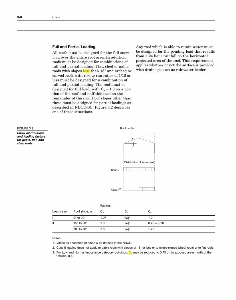
All roofs must be designed for the full snow load over the entire roof area. In addition, roofs must be designed for combinations of full and partial loading. Flat, shed or gable roofs with slopes less than 15° and arched or curved roofs with rise to run ratios of 1/10 or less must be designed for a combination of full and partial loading. The roof must be designed for full load, with Ca = 1.0 on a por-tion of the roof and half this load on the remainder of the roof. Roof slopes other than these must be designed for partial loadings as described in NBCC-SC. Figure 3.2 describes one of these situations.
Any roof which is able to retain water must be designed for the ponding load that results from a 24 hour rainfall on the horizontal projected area of the roof. This requirement applies whether or not the surface is provided with drainage such as rainwater leaders.
Factors
Load case Roof slope, α Cw Cs Ca
I 0° to 90° 1.03 f(α)1 1.0
II 15° to 20° 1.0 f(α)1 0.25 + α/20
20° to 90° 1.0 f(α)1 1.25
Notes:
1. Varies as a function of slope α as defined in the NBCC.
2. Case II loading does not apply to gable roofs with slopes of 15° or less or to single-sloped (shed) roofs or to flat roofs.
3. For Low and Normal Importance category buildings, Cw may be reduced to 0.75 or, in exposed areas north of the treeline, 0.5.
Wind and EarthquakE Loads
Both wind and earthquake loads are highly variable, and sound engineering judgement is very important to arrive at a rational design solution. It should also be realized that both are dynamic load conditions.
For large or irregular-shaped structures, dynamic analysis or wind tunnel testing may be required to adequately account for wind and seismic loads. Wood buildings tend to be relatively rigid and not too tall or slender. For these reasons, a simplified approach using equivalent static loads can usually be used.
Wind Load
The effect of high winds acting over the large areas of buildings can result in substantial lateral loads (Figure 3.3).
In the NBCC there are three separate approaches for determining design wind loads on buildings.
The Dynamic Procedure is intended for primarily tall buildings and slender struc-tures. The Experimental Procedure consists of wind tunnel testing and other experimental methods. These methods are further discussed in the NBCC Structural Commentaries.
The static procedure is appropriate for use with the majority of wind loadings and types of structures, including the structure and cladding of low-and medium-rise buildings (which are fairly rigid), and the cladding of high-rise buildings.
FIguRe 3.2
Snow distributions and loading factors for gable, flat, and shed roofs
Roof pro�le
Distribution of snow load
Case I
Case II(2)
α
FIguRe 3.3
Wind effects
α
External Pressures
Internal Pressures
6-26 Wood Products
WOOD I-JOISTS
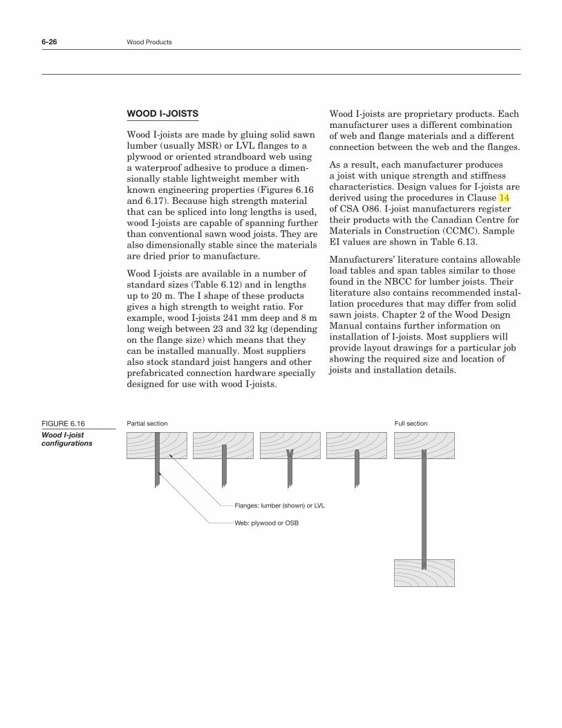
Wood I-joists are made by gluing solid sawn lumber (usually MSR) or LVL flanges to a plywood or oriented strandboard web using a waterproof adhesive to produce a dimen-sionally stable lightweight member with known engineering properties (Figures 6.16 and 6.17). Because high strength material that can be spliced into long lengths is used, wood I-joists are capable of spanning further than conventional sawn wood joists. They are also dimensionally stable since the materials are dried prior to manufacture.
Wood I-joists are available in a number of standard sizes (Table 6.12) and in lengths up to 20 m. The I shape of these products gives a high strength to weight ratio. For example, wood I-joists 241 mm deep and 8 m long weigh between 23 and 32 kg (depending on the flange size) which means that they can be installed manually. Most suppliers also stock standard joist hangers and other prefabricated connection hardware specially designed for use with wood I-joists.
Wood I-joists are proprietary products. Each manufacturer uses a different combination of web and flange materials and a different connection between the web and the flanges.
As a result, each manufacturer produces a joist with unique strength and stiffness characteristics. Design values for I-joists are derived using the procedures in Clause 14 of CSA O86. I-joist manufacturers register their products with the Canadian Centre for Materials in Construction (CCMC). Sample EI values are shown in Table 6.13.
Manufacturers’ literature contains allowable load tables and span tables similar to those found in the NBCC for lumber joists. Their literature also contains recommended instal-lation procedures that may differ from solid sawn joists. Chapter 2 of the Wood Design Manual contains further information on installation of I-joists. Most suppliers will provide layout drawings for a particular job showing the required size and location of joists and installation details.
FIGURE 6.16
Wood I-joist configurations
Web: plywood or OSB
Flanges: lumber (shown) or LVL
Partial section Full section
6-32 Wood Products
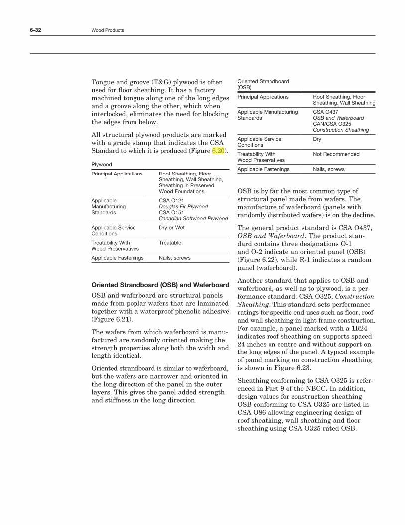
Tongue and groove (T&G) plywood is often used for floor sheathing. It has a factory machined tongue along one of the long edges and a groove along the other, which when interlocked, eliminates the need for blocking the edges from below.
All structural plywood products are marked with a grade stamp that indicates the CSA Standard to which it is produced (Figure 6.20).
Plywood
Principal Applications Roof Sheathing, Floor Sheathing, Wall Sheathing, Sheathing in Preserved Wood Foundations
Applicable Manufacturing Standards
CSA O121 Douglas Fir Plywood CSA O151 Canadian Softwood Plywood
Applicable Service Conditions
Dry or Wet
Treatability With Wood Preservatives
Treatable
Applicable Fastenings Nails, screws
Oriented Strandboard (OSB) and Waferboard
OSB and waferboard are structural panels made from poplar wafers that are laminated together with a waterproof phenolic adhesive (Figure 6.21).
The wafers from which waferboard is manufactured are randomly oriented making the strength properties along both the width and length identical.
Oriented strandboard is similar to waferboard, but the wafers are narrower and oriented in the long direction of the panel in the outer layers. This gives the panel added strength and stiffness in the long direction.
Oriented Strandboard (OSB)
Principal Applications Roof Sheathing, Floor Sheathing, Wall Sheathing
Applicable Manufacturing Standards
CSA O437 OSB and Waferboard CAN/CSA O325 Construction Sheathing
Applicable Service Conditions
Dry
Treatability With Wood Preservatives
Not Recommended
Applicable Fastenings Nails, screws
OSB is by far the most common type of structural panel made from wafers. The manufacture of waferboard (panels with randomly distributed wafers) is on the decline.
The general product standard is CSA O437, OSB and Waferboard. The product standard contains three designations O1 and O2 indicate an oriented panel (OSB) (Figure 6.22), while R1 indicates a random panel (waferboard).
Another standard that applies to OSB and waferboard, as well as to plywood, is a performance standard: CSA O325, Construction Sheathing. This standard sets performance ratings for specific end uses such as floor, roof and wall sheathing in lightframe construction. For example, a panel marked with a 1R24 indicates roof sheathing on supports spaced 24 inches on centre and without support on the long edges of the panel. A typical example of panel marking on construction sheathing is shown in Figure 6.23.
Sheathing conforming to CSA O325 is referenced in Part 9 of the NBCC. In addition, design values for construction sheathing OSB conforming to CSA O325 are listed in CSA O86 allowing engineering design of roof sheathing, wall sheathing and floor sheathing using CSA O325 rated OSB.
8-3Introduction to Wood Design
INTRODUCTION
The load carrying capacity of an axially loaded wood compression member depends on both the compression strength of the wood and on stability. Column stability in turn depends on stiffness which is affected by the slenderness of the member.
For wood columns, which are usually rect-angular in shape, the slenderness ratio shall be calculated for both axes. The measure of slenderness, Cc, is the ratio of the effective length to the associated dimension. The effective length is used to account for conditions of end restraint considering the possible buckled shape for a given column.
As slenderness increases, load carrying capacity decreases (as a cubic function of slenderness) so that a short column can support more load than a long column of the same cross section, grade and species. The size effect on material strength also affects columns and is taken into account separately from slenderness by using the factor KZc.
SAWN LUMBER COLUMNS
For sawn lumber, the slenderness ratio, Cc, is restricted to a maximum value of 50 (at which sawn lumber columns may have only about 10 to 25% of the capacity they have at a slenderness ratio of about 5).
The slenderness factor, KC, is used to relate slenderness to load capacity for lumber columns. The formulation used for KC in CSA O86 is one based on a cubic Rankine-Gordon expression. The reliability assessments leading to selecting the performance factor, ϕ, for lumber columns incorporated a nominal load eccentricity of 5% of the member width, on average.
To design a sawn lumber column to support a given factored load, determine the effective length, select a member size, grade and species group and calculate the factored compressive resistance parallel to grain for both areas. If the resistance is less than the load, select another size and recalculate.
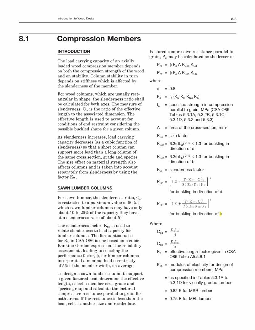
Factored compressive resistance parallel to grain, Pr, may be calculated as the lesser of
Prd = ϕ Fc A KZcd KCd
Prb = ϕ Fc A KZcb KCb
where
ϕ = 0.8
Fc = fc (KD KH KSC KT)
fc = specified strength in compression parallel to grain, MPa (CSA O86 Tables 5.3.1A, 5.3.2B, 5.3.1C, 5.3.1D, 5.3.2 and 5.3.3)
A = area of the cross-section, mm2
KZc = size factor
KZcd = 6.3(dLd)-0.13 ≤ 1.3 for buckling in direction of d
KZcb = 6.3(bLb)-0.13 ≤ 1.3 for buckling in direction of b
KC = slenderness factor
KCd = –
1.0 35E K KF K C
05 SE T
C ZCd Cd3 1
+; E for buckling in direction of d
KCb = –
1.0 35E K KF K C
05 SE T
C ZCb Cb3 1
+; E for buckling in direction of b
Where
Ccd = d
K Le d
Ccb = bK Le b
Ke = effective length factor given in CSA O86 Table A5.5.6.1
E05 = modulus of elasticity for design of compression members, MPa
= as specified in Tables 5.3.1A to 5.3.1D for visually graded lumber
= 0.82 E for MSR lumber
= 0.75 E for MEL lumber
8.1 Compression Members
11-63Introduction to Wood Design
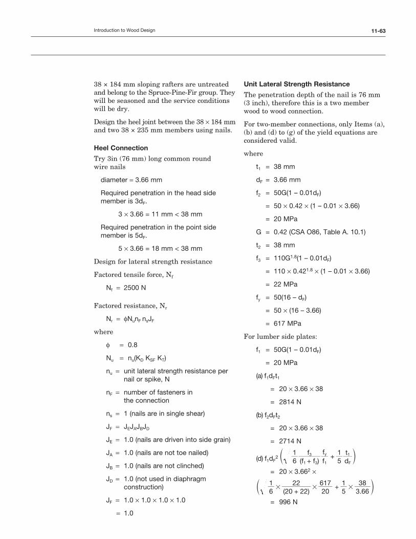
38 × 184 mm sloping rafters are untreated and belong to the Spruce-Pine-Fir group. They will be seasoned and the service conditions will be dry.
Design the heel joint between the 38 × 184 mm and two 38 × 235 mm members using nails.
Heel Connection
Try 3 in (76 mm) long common round wire nails
diameter = 3.66 mm
Required penetration in the head side member is 3 dF.
3 × 3.66 = 11 mm < 38 mm
Required penetration in the point side member is 5 dF.
5 × 3.66 = 18 mm < 38 mm
Design for lateral strength resistance
Factored tensile force, Nf
Nf = 2500 N
Factored resistance, Nr
Nr = ϕNunF nsJF
where
ϕ = 0.8
Nu = nu(KD KSF KT)
nu = unit lateral strength resistance per nail or spike, N
nF = number of fasteners in the connection
ns = 1 (nails are in single shear)
JF = JEJAJBJD
JE = 1.0 (nails are driven into side grain)
JA = 1.0 (nails are not toe nailed)
JB = 1.0 (nails are not clinched)
JD = 1.0 (not used in diaphragm construction)
JF = 1.0 × 1.0 × 1.0 × 1.0
= 1.0
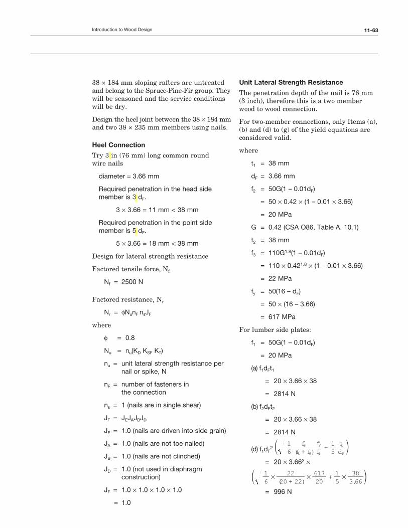
Unit Lateral Strength Resistance
The penetration depth of the nail is 76 mm (3 inch), therefore this is a two member wood to wood connection.
For two-member connections, only Items (a), (b) and (d) to (g) of the yield equations are considered valid.
where
t1 = 38 mm
dF = 3.66 mm
f2 = 50G(1 – 0.01dF)
= 50 × 0.42 × (1 – 0.01 × 3.66)
= 20 MPa
G = 0.42 (CSA O86, Table A. 10.1)
t2 = 38 mm
f3 = 110G1.8(1 – 0.01dF)
= 110 × 0.421.8 × (1 – 0.01 × 3.66)
= 22 MPa
fy = 50(16 – dF)
= 50 × (16 – 3.66)
= 617 MPa
For lumber side plates:
f1 = 50G(1 – 0.01dF)
= 20 MPa
(a) f1dFt1
= 20 × 3.66 × 38
= 2814 N
(b) f2dFt2
= 20 × 3.66 × 38
= 2814 N
(d) f1dF2 6
1(f f)f
ff
51dt
+ +1 3
3
1
y
F
1c m
= 20 × 3.662 ×
61
(20 22)22
20617
51
3.6638
+ +# # #c m
= 996 N
11-64 Connections
(e) f1dF2
2
61(f f)f
ff
51dt
+ +1 3
3
1
y
Fc m
= 20 × 3.662 ×
61
(20 22)22
20617
51
3.6638
+ +# # #c m
= 996 N
(f) f1dF2
51
dt
ffdt+
F
1
1
2
F
2` j
= 51 × 20 × 3.662 ×
3.6638
2020
3.6638+ #` j
= 1113 N
(g) f1dF2 3
2(f f)f
ff
+1 3
3
1
y
= 20 × 3.662 ×
32
(20 22)22
20617
+# #
= 879 N (Governs)
Therefore, based on the above unit yield equations, nu = 879 N.
Nu = nu(KDKSFKT)
= 879 × (1.0 x 1.0 x 1.0)
= 879 N
Nr = N nn Jz u f s F
= 0.8 x 879 x nF x 1 1.0
= 703 nF (N)
Nr ≥ Nf
703 nF ≥ 2500 N
nF ≥ 3.6
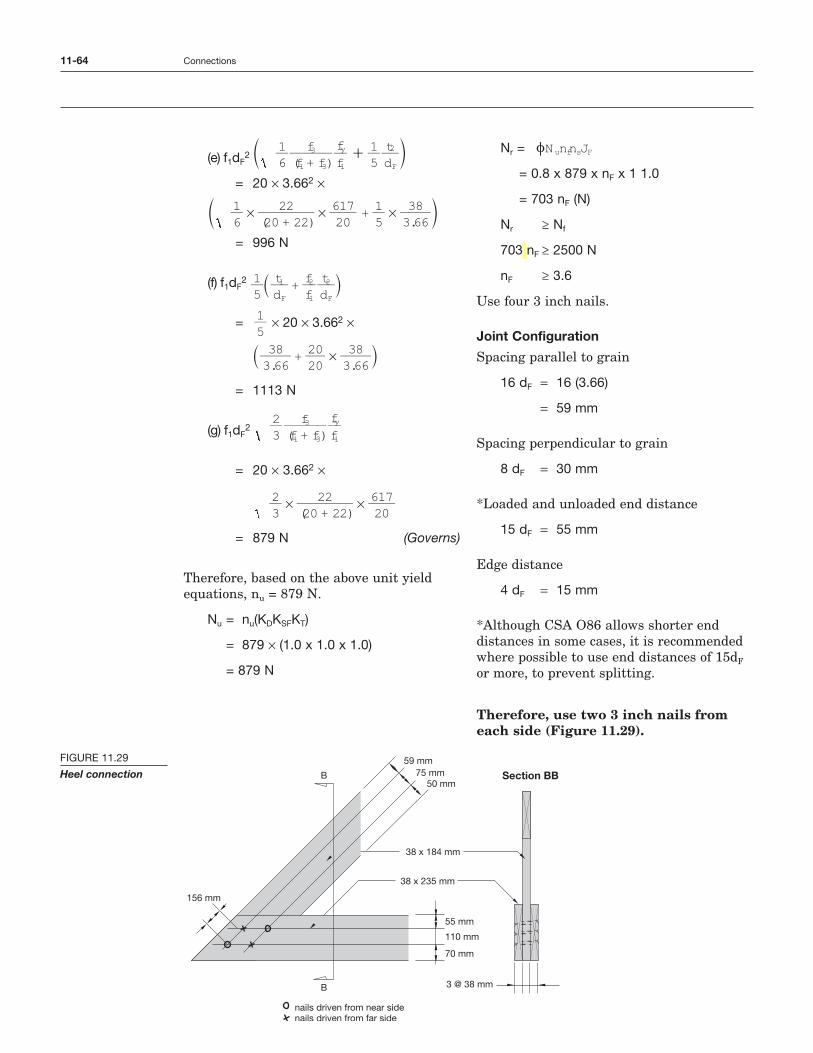
Use four 3 inch nails.
Joint Configuration
Spacing parallel to grain
16 dF = 16 (3.66)
= 59 mm
Spacing perpendicular to grain
8 dF = 30 mm
*Loaded and unloaded end distance
15 dF = 55 mm
Edge distance
4 dF = 15 mm
*Although CSA O86 allows shorter end distances in some cases, it is recommended where possible to use end distances of 15dF or more, to prevent splitting.
Therefore, use two 3 inch nails from each side (Figure 11.29).
FIGURE 11.29
Heel connection
38 x 184 mm
38 x 235 mm
nails driven from near sidenails driven from far side
B Section BB
55 mm
110 mm
70 mm
59 mm75 mm
50 mm
3 @ 38 mmB
156 mm
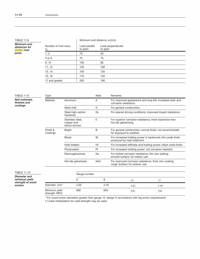
11-74 Connections
Minimum end distance, a (mm)
Number of rivet rows, nR
Load parallel to grain
Load perpendicular to grain
1, 2 75 50
3 to 8 75 75
9, 10 100 80
11, 12 125 100
13, 14 150 120
15, 16 175 140
17 and greater 200 160
TABLE 11.8
Minimum end distances for timber rivet joints
Type Abbr. Remarks
Material Aluminum A For improved appearance and long life; increased stain and corrosion resistance.
Steel-mild S For general construction.
Steel-high-carbon hardened
Sc For special driving conditions; improved impact resistance.
Stainless steel, copper and silicon-bronze
E For superior corrosion resistance; more expensive than hot-dip galvanizing.
Finish & Coatings
Bright B For general construction; normal finish; not recommended for exposure to weather.
Blued Bl For increased holding power in hardwood; thin oxide finish produced by heat treatment.
Heat treated Ht For increased stiffness and holding power; black oxide finish.
Phoscoated Pt For increased holding power; not corrosion resistant.
Electrogalvanized Ge For limited corrosion resistance; thin zinc plating; smooth surface; for interior use.
Hot-dip galvanized Ghd For improved corrosion resistance; thick zinc coating; rough surface; for exterior use.
TABLE 11.9
Nail materials, finishes and coatings
Gauge number
6 8 10 12
Diameter, mm* 3.50 4.16 4.82 5.48
Minimum yield strength, MPa†
690 620 550 550
* For wood screw diameters greater than gauge 12, design in accordance with lag screw requirements.† Linear interpolation for yield strength may be used.
TABLE 11.10
Diameter and minimum yield strength of wood screws
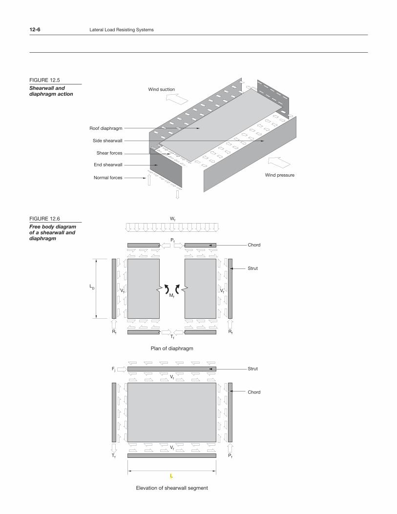
12-6 Lateral Load Resisting Systems
FIGURE 12.5
Shearwall and diaphragm action
Shear forces
Normal forces
Roof diaphragm
Wind pressure
Wind suction
Side shearwall
End shearwall
FIGURE 12.6
Free body diagram of a shearwall and diaphragm
Wf
Pf
Mf
VfVf
Vf
Vf
Tf Pf
Rf
Fj
RfTf
Plan of diaphragm
Chord
Elevation of shearwall segment
Strut
Strut
Chord
LD
L
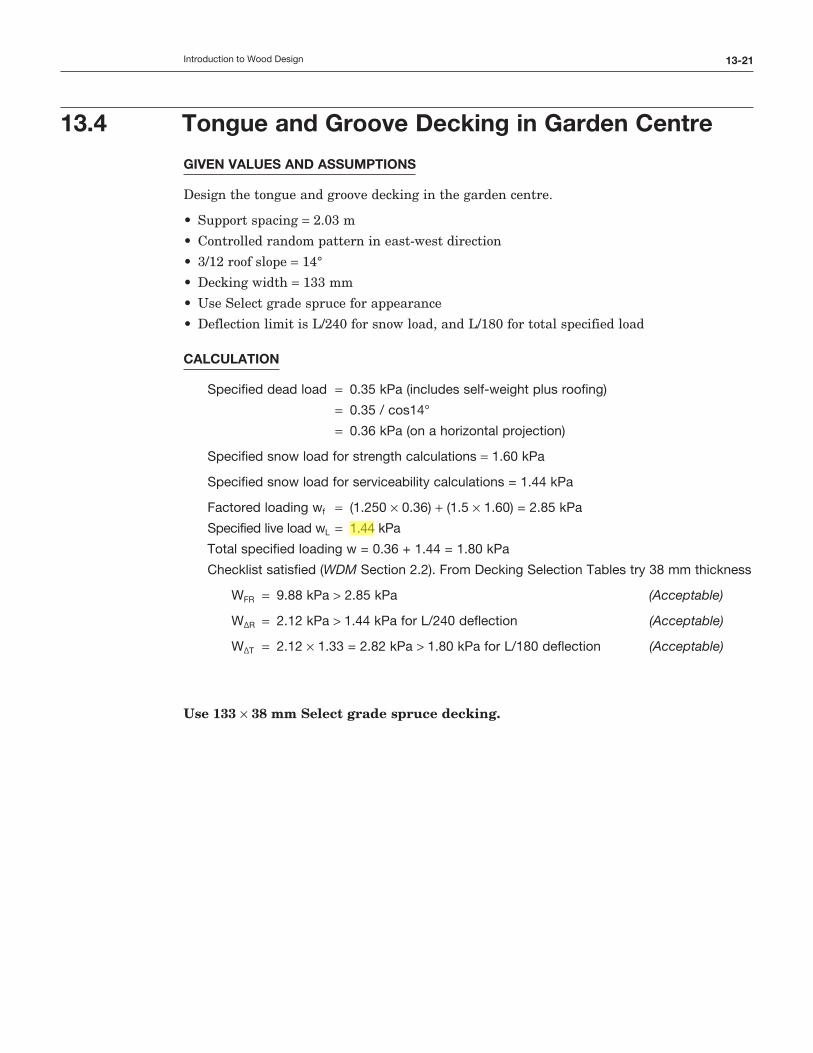
13-21Introduction to Wood Design
13.4 Tongue and Groove Decking in Garden Centre
GIVEN VALUES AND ASSUMPTIONS
Design the tongue and groove decking in the garden centre.
• Support spacing = 2.03 m
• Controlled random pattern in east-west direction
• 3/12 roof slope = 14°
• Decking width = 133 mm
• Use Select grade spruce for appearance
• Deflection limit is L/240 for snow load, and L/180 for total specified load
CALCULATION
Specified dead load = 0.35 kPa (includes self-weight plus roofing)
= 0.35 / cos14°
= 0.36 kPa (on a horizontal projection)
Specified snow load for strength calculations = 1.60 kPa
Specified snow load for serviceability calculations = 1.44 kPa
Factored loading wf = (1.250 × 0.36) + (1.5 × 1.60) = 2.85 kPa
Specified live load wL = 1.44 kPa
Total specified loading w = 0.36 + 1.44 = 1.80 kPa
Checklist satisfied (WDM Section 2.2). From Decking Selection Tables try 38 mm thickness
WFR = 9.88 kPa > 2.85 kPa (Acceptable)
W∆R = 2.12 kPa > 1.44 kPa for L/240 deflection (Acceptable)
W∆T = 2.12 × 1. 33 = 2.82 kPa > 1.80 kPa for L/180 deflection (Acceptable)
Use 133 × 38 mm Select grade spruce decking.
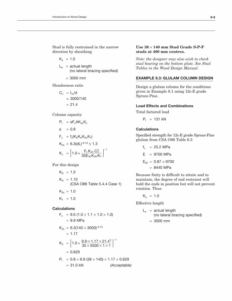
8-9Introduction to Wood Design
Stud is fully restrained in the narrow direction by sheathing
Ke = 1.0
Le = actual length (no lateral bracing specified)
= 3000 mm
Slenderness ratio
Cc = Le/d
= 3000/140
= 21.4
Column capacity
Pr = ϕFcAKZcKc
ϕ = 0.8
Fc = fc(KDKHKScKT)
KZc = 6.3(dL)-0.13 ≤ 1.3
Kc = 1.035E K KF K C
05 SE T
c Zc C3 – 1
+; E
For this design
KD = 1.0
KH = 1.10 (CSA O86 Table 5.4.4 Case 1)
KSc = 1.0
KT = 1.0
Calculations
Fc = 9.0 (1.0 × 1.1 × 1.0 × 1.0)
= 9.9 MPa
KZc = 6.3(140 × 3000)-0.13
= 1.17
KC = 1.035 5500 1 1
1.17 21.4.9 9 3 – 1
+# # ## #; E
= 0.629
Pr = 0.8 × 9.9 (38 × 140) × 1.17 × 0.629
= 31.0 kN (Acceptable)
Use 38 × 140 mm Stud Grade S-P-F studs at 400 mm centres.
Note: the designer may also wish to check stud bearing on the bottom plate. See Stud Tables in the Wood Design Manual.
exaMpLe 8.3: GLuLaM CoLuMn deSIGn
Design a glulam column for the conditions given in Example 8.1 using 12c-E grade Spruce-Pine.
Load effects and Combinations
Total factored load
Pf = 131 kN
Calculations
Specified strength for 12c-E grade Spruce-Pine glulam from CSA O86 Table 6.3
fc = 25.2 MPa
E = 9700 MPa
E05 = 0.87 × 9700
= 8440 MPa
Because fixity is difficult to attain and to maintain, the degree of end restraint will hold the ends in position but will not prevent rotation. Thus:
Ke = 1.0
Effective length
Le = actual length (no lateral bracing specified)
= 3000 mm
11-63Introduction to Wood Design
38 × 184 mm sloping rafters are untreated and belong to the Spruce-Pine-Fir group. They will be seasoned and the service conditions will be dry.
Design the heel joint between the 38 × 184 mm and two 38 × 235 mm members using nails.
heel Connection
Try 3in (76 mm) long common round wire nails
diameter = 3.66 mm
Required penetration in the head side member is 3dF.
3 × 3.66 = 11 mm < 38 mm
Required penetration in the point side member is 5dF.
5 × 3.66 = 18 mm < 38 mm
Design for lateral strength resistance
Factored tensile force, Nf
Nf = 2500 N
Factored resistance, Nr
Nr = ϕNunF nsJF
where
ϕ = 0.8
Nu = nu(KD KSF KT)
nu = unit lateral strength resistance per nail or spike, N
nF = number of fasteners in the connection
ns = 1 (nails are in single shear)
JF = JeJAJBJD
Je = 1.0 (nails are driven into side grain)
JA = 1.0 (nails are not toe nailed)
JB = 1.0 (nails are not clinched)
JD = 1.0 (not used in diaphragm construction)
JF = 1.0 × 1.0 × 1.0 × 1.0
= 1.0
unit Lateral Strength Resistance
The penetration depth of the nail is 76 mm (3 inch), therefore this is a two member wood to wood connection.
For two-member connections, only Items (a), (b) and (d) to (g) of the yield equations are considered valid.
where
t1 = 38 mm
dF = 3.66 mm
f2 = 50G(1 – 0.01dF)
= 50 × 0.42 × (1 – 0.01 × 3.66)
= 20 MPa
G = 0.42 (CSA O86, Table A. 10.1)
t2 = 38 mm
f3 = 110G1.8(1 – 0.01dF)
= 110 × 0.421.8 × (1 – 0.01 × 3.66)
= 22 MPa
fy = 50(16 – dF)
= 50 × (16 – 3.66)
= 617 MPa
For lumber side plates:
f1 = 50G(1 – 0.01dF)
= 20 MPa
(a) f1dFt1
= 20 × 3.66 × 38
= 2814 N
(b) f2dFt2
= 20 × 3.66 × 38
= 2714 N
(d) f1dF2
61
(f f )f
ff
51
dt
++
1 3
3
1
y
F
1c m
= 20 × 3.662 ×
61
(20 22)22
20617
51
3.6638
++# # #c m
= 996 N
12-18 Lateral Load Resisting Systems
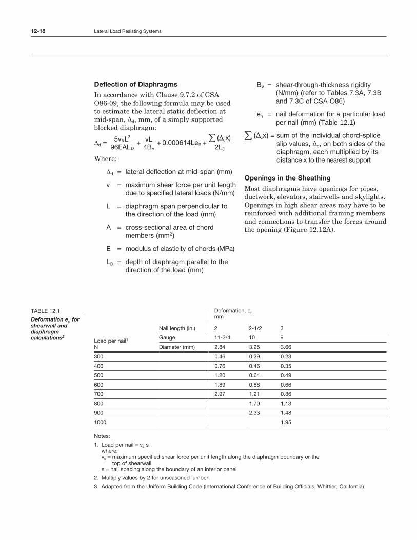
Deflection of Diaphragms
In accordance with Clause 9.7.2 of CSA O86-09, the following formula may be used to estimate the lateral static deflection at mid-span, Δd, mm, of a simply supported blocked diaphragm:
Δd = 96EAL5v L
4BvL 0.000614Le
2L( x)
D
s3
vn+ + +
D
D
c/
Where:
Δd = lateral deflection at mid-span (mm)
v = maximum shear force per unit length due to specified lateral loads (N/mm)
L = diaphragm span perpendicular to the direction of the load (mm)
A = cross-sectional area of chord members (mm2)
E = modulus of elasticity of chords (MPa)
LD = depth of diaphragm parallel to the direction of the load (mm)
BV = shear-through-thickness rigidity (N/mm) (refer to Tables 7.3A, 7.3B and 7.3C of CSA O86)
en = nail deformation for a particular load per nail (mm) (Table 12.1)
( x)Dc/ = sum of the individual chord-splice slip values, Δc, on both sides of the diaphragm, each multiplied by its distance x to the nearest support
Openings in the Sheathing
Most diaphragms have openings for pipes, ductwork, elevators, stairwells and skylights. Openings in high shear areas may have to be reinforced with additional framing members and connections to transfer the forces around the opening (Figure 12.12A).
TABLE 12.1
Deformation en for shearwall and diaphragm calculations2
Deformation, en mm
Nail length (in.) 2 2-1/2 3
Load per nail1 N
Gauge 11-3/4 10 9
Diameter (mm) 2.84 3.25 3.66
300 0.46 0.29 0.23
400 0.76 0.46 0.35
500 1.20 0.64 0.49
600 1.89 0.88 0.66
700 2.97 1.21 0.86
800 1.70 1.13
900 2.33 1.48
1000 1.95
Notes:
1. Load per nail = vs s where: vs = maximum specified shear force per unit length along the diaphragm boundary or the
top of shearwall s = nail spacing along the boundary of an interior panel
2. Multiply values by 2 for unseasoned lumber.
3. Adapted from the uniform Building Code (International Conference of Building Officials, Whittier, California).
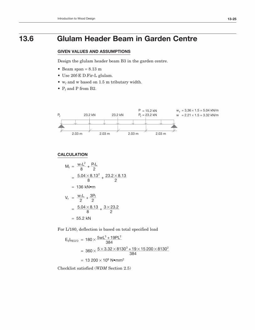
13-25Introduction to Wood Design
GIveN vALUeS AND ASSUMPTIoNS
Design the glulam header beam B3 in the garden centre.
• Beam span = 8.13 m
• Use 20f‑E D.Fir‑L glulam.
• wf and w based on 1.5 m tributary width.
• Pf and P from B2.
CALCULATIoN
Mf = 8
w L2LPf
2f+
= 8
5.04 8.12
23. 8.13 2 32+# #
= 136kN•m
Vf = w L2P3
2f f+
= 5.04 8.12
3 23.8
3 2+# #
= 55.2 kN
For L/180, deflection is based on total specified load
ESIREQ’D = 180384
5wL 19PL3 2+#
= 360384
5 3.32 81 0 19 15 00 81 03 2 33 2+# # # # #
= 13 200 × 109N•mm2
Checklist satisfied (WDM Section 2.5)
13.6 Glulam Header Beam in Garden Centre
Pf
w = 3.36 × 1.5 = 5.04 kN/mf23.2 kN 23.2 kN = 23.2 kNPf
P = 15.2 kN
2.03 m2.03 m2.03 m2.03 m
w = 2.21 × 1.5 = 3.32 kN/m