Full Report3

8/3/2019 Full Report3

http://slidepdf.com/reader/full/full-report3 1/70

1

CONTENTS

1. Abstract«««««««««««««««««««««««««««.4

2. Introduction««««««««««««««««««««««««..«5

2.1 Low Frequency Oscillations In Power Systems«««««««««..5

2.2 Fixed Parameter Controllers«««««««««««««««.......7

2.2.1 Conventional Stabilizers««««««««««««««««.«8

2.2.2 Other Fixed Parameter Controllers««««««««««««..9

2.2.3 The Drawbacks Of Conventional Fixed Parameter Controllers«10

2.3 Adaptive Controllers««««««««««««««««««««.10

2.4 Fuzzy Logic Controllers«««««««««««««««««««12

2.5 Artificial Neural Network ««««««««««««««««««13

2.5.1 Artificial Neural Network as a Controller«««««««««...14

2.5.2 Artificial Neural Network as a Parameter Identifier«««««..15

2.6 Scope of Present Work«««««««««««««««««««.16

3. Power System Stabilizers(PSS)««««««««««««««««««.17

3.1 Power System Stability«««««««««««««««««««17



2

3.2 Power system stabilizer««««««««««««««««««19

3.3 System investigated«««««««««««««««««««..21

3.4 Transfer function model of the power system stabilizer and the

Design Considerations««««««««««««««««««.22

3.4.1 Phase lead compensation««««««««««««««...23

3.4.2 Stabilizing signal washout««««««««««««««..23

3.4.3 Stabilizer gain«««««««««««««««««««.23

3.5 Modeling of a single machine system connected to infinite bus

System««««««««««««««««««««««««...24

4. Artificial Neural Network(ANN)«««««««««««««««««28

4.1 Neuron Model«««««««««««««««««««««..29

4.2 Characteristics of artificial neural networks««««««««..32

4.3 Learning methods««««««««««««««««««««32

4.4 Backpropagation««««««««««««««««««««.36

4.4.1Feed forward network«««««««««««««««.38

4.4.2recurrent network«««««««««««««««««39

4.4.3 Levenberg-Marquardt algorithm««««««««««..40



3

4.5 Backpropagation learning algorithm««««««««««««.41

5. Mathematical modeling«««««««««««««««««««««.45

6. Experimental investigations«««««««««««««««««««.49

7. Experimental results««««««««««««««««««««««.60

8. Discussion of experimental results and experimental investigations««..61

9. Conclusions««««««««««««««««««««««««««62

10. References«««««««««««««««««««««««««...64

11. Appendix««««««««««««««««««««««««««..69



4

ABSTRACT

The problem of dynamic stability of power system has challenged power system

engineers since over three decades now. The application of Power System Stabilizer (PSS) can

help in damping out low frequency oscillations and improve the system stability. The traditional

and till date the most popular solution to this problem is application of conventional power

system stabilizer (CPSS). However, continual changes in the operating condition and network

parameters result in corresponding change in system dynamics. This constantly changing nature

of power system makes the design of CPSS a difficult task.

This project work presents a systematic approach for designing a self-tuning adaptive

power system stabilizer (PSS) based on artificial neural network (ANN). An ANN is used for

self-tuning the parameters of PSS e.g. stabilizing gain K stab and time constant (T1) for Lead PSS

in real-time. The inputs to the ANN are generator terminal active power (P) and reactive power

(Q). Investigations are carried out to assess the dynamic performance of the system with self-

tuning PSS based on ANN (ST-ANNPSS) over a wide range of loading conditions.



5

2.INTRODUCTION

2.1 Low Frequency Oscillations in Power System:

Small oscillations in power systems were observed as far back as the early twenties of

this century. The oscillations were described as hunting of synchronous machines. In a generator,

the electro-mechanical coupling between the rotor and the rest of the system causes it to behave

in a manner similar to a spring-mass-damper system which exhibits oscillatory behaviour

following any disturbance from the equilibrium state.

Small oscillations were a matter of concern, but for several decades power system

engineers remained preoccupied with transient stability. That is the stability of the system

following large disturbances. Causes for such disturbances were easily identified and remedial

measures were devised. In early sixties, most of the generators were getting interconnected and

the automatic voltage regulators (AVRs) were more efficient. With bulk power transfer on long

and weak transmission lines and application of high gain, fast acting AVRs, small oscillations of

even lower frequencies were observed. These were described as Inter-Tie oscillations. Some

times oscillations of the generators within the plant were also observed. These oscillations at

slightly higher frequencies were termed as Intra-Plant oscillations.

The combined oscillatory behavior of the system encompassing the three modes of

oscillations are popularly called the dynamic stability of the system. In more precise terms it is

known as the small signal oscillatory stability of the system.



6

A power system is said to be small signal stable for a particular steady-state operating

condition if, following any small disturbance, it reaches a steady state operating condition which

is identical or close to the pre-disturbance operating condition."

The oscillations, which are typically in the frequency range of 0.2 to 3.0 Hz. might be

excited by disturbances in the system or, in some cases, might even build up spontaneously.

These oscillations limit the power transmission capability of a network and, sometimes, may

even cause loss of synchronism and an eventual breakdown of the entire system. In practice, in

addition to stability, the system is required to be well damped i.e. the oscillations, when excited,

should die down within a reasonable amount of time.

Reduction in power transfer levels and AVR gains does curb the oscillations and is often

resorted to during system emergencies. These are however not feasible solutions to the problem.

The stability of the system, in principle, can be enhanced substantially by application of some

form of close-loop feedback control. Over the years a considerable amount of effort has been

extended in laboratory research and on-site studies for designing such controllers.

There are basically three following ways by which the stability of the system can be

improved,

(1) Using supplementary control signals in the generator excitation system.

(2) Making use of fast valving technique in steam turbine.

(3) Impedance Control-resistance breaking and application of the FACTS devices, etc.



7

The problem, when first encountered, was solved by fitting the generators with a

feedback controller which sensed the rotor slip or change in terminal power of the generator and

fed it back at the AVR reference input with proper phase lead and magnitude so as to generate an

additional damping torque on the rotor [1]. This device came to be known as a Power System

Stabilizer (PSS).

Damping power oscillations using supplementary controls through turbine, governor loop

had limited success. With the advent fast valving technique, there is some renewed interest in

this type of control [2].

There can also be other kinds of controls applied to the system for counteracting the

oscillatory behaviour - for instance FACTS devices can be fitted with supplementary controllers

which improve the system stability.

Power system stabilizers are now routinely used in the industry. However, the complex,

constantly changing nature of power systems has severely restricted the efficacy of these devices.

2.2 Fixed Parameter Controllers:

Over the years, a number of techniques have been developed for designing PSSs and

other damping controllers [3]. Some of these stabilizing methods have been briefly described in



8

this section. The main motivation for including this rather brief exposition of the existing

techniques is to introduce the need for the application of robust control techniques in power

systems. Some of references cited here include a more comprehensive coverage of the topic.

2.2.1 Conventional Stabilizers:

The earlier stabilizer designs were based on concepts derived from classical control

theory [4-8]. Many such designs have been physically realized and widely used in actual

systems. These controllers feedback suitably phase compensated signals derived from the power,

speed and frequency of the operating generator either alone or in various combination as input

signals so as to generate an additional rotor torque to damp out the low frequency oscillations.

The gain and the required phase lead/lag of the stabilizers are `tuned' by using appropriate

mathematical models, supplemented by a good understanding of the system operation.

The principles of operation of this controller are based on the concepts of damping and

synchronizing torques within the generator. A comprehensive analysis of this torques has been

dealt with by deMello and Concordia in their landmark paper in 1969 [1]. These controllers have

been known to work quite well in the field and are extremely simple to implement. However, the

tuning of these compensators continues to be a formidable task especially in large multi-machine

systems with multiple oscillatory modes. Larsen and Swann, in their three part paper [6],

describe in detail the general tuning procedure for this type of stabilizers.

PSS design using this method involves some amount of trial and error and experience on

part of the designer. Further these controllers are tuned for particular operating conditions and



9

with change in operating conditions they require re-tuning. Robustness issues are also not

adequately addressed in this classical setting.

2.2.2 Other Fixed Parameter Controllers:

There have also been numerous attempts at applying various other control strategies in

particular modal control [9-11] and LQ optimal control [12, 13] techniques for designing

damping controllers. These attempts exemplify the growing preference for algorithmic controller

design methods as opposed to the classical intuitive ones. They call for a lesser amount of

engineering judgment and experience on part of the designer. The ill-suited ness of the quadratic

performance index used in LQR/LQG to the problem has motivated researchers to define

alternative performance indices which aptly capture the magnitude of system damping [14, 15].

Such indices can be optimized using standard numerical optimization techniques [16].

These techniques have the advantage of being straight forward and algorithmic with little

ambiguity in the recommended procedure. A few extensions of these methods tried to

incorporate some robustness by optimizing some additional index such as eigen value

sensitivities. Sensitivity minimization in this form, though, quite helpful as a means of providing

robustness in the absence of better methods is essentially a qualitative approach and hence does

not guarantee performance preservation in the face of modal inaccuracies [17].



10

2.2.3 The Drawbacks of Conventional Fixed Parameter Controllers:

The main drawback of the above controllers is their inherent lack of robustness. Power

systems continually undergo changes in the load and generation patterns and in the transmission

network. This results in an accompanying change in small signal dynamics of the system. The

fixed parameter controllers, tuned for a particular operating condition, usually give good

performance at that operating condition. Their performance, at other operating conditions, may at

best be satisfactory, and may even become inadequate when extreme situations arise. However

such stabilizers have been very useful in system that could be represented by single machine

infinite bus models. In interconnected multi-machine systems the dynamic instability can

manifest itself in the form of poorly damped oscillation of one particular unit with the rest of the

system or a group, or a group of machines oscillating against another group of machines. Thus, a

generating unit in a multi-machine environment often participates in both `local' and `inter-area'

modes of oscillations simultaneously. The spectral and temporal distributions of these modes are

largely determined by the rest of the system. As the operating conditions and system

configuration are constantly changing in actual power system the performance of the fixed

parameter stabilizers can not be always guaranteed.

2.3 Adaptive Controllers:

The problem of changing system dynamics due to changes in the operating conditions

can be handled by the application of adaptive control [18, 19]. The power system can be

continuously monitored and the controller parameters can be updated in real time to maintain

specified performance inspite of changes in the system dynamics. All three standard methods of

adaptive control listed below have been tried for designing power system stabilizers.



11

(a) Model reference adaptive control (MRAC) [20, 21]

(b) Self tuning control (STC) [22-24]

(c) Gain scheduling adaptive control (GSAC) [25]

In MRAC, the desired behavior of the closed loop system is incorporated in a reference

model. With the plant and the reference model excited by the same input, the error between the

plant output and the reference model output is used to modify the controller parameters, such that

the plant is driven to match the behavior of the reference model.

In STC, at every sampling instant, the parameters of an assumed model for the plant are

identified using some suitable algorithms, such as Recursive least squares (RLS) or Maximum

likelihood estimator etc. The identified parameters are then used in control laws which could be

based on various popular techniques such as pole-shifting, pole placement etc.

In GSAC, the gains of the controller are adjusted according to a variety of innovative

control strategies depending upon the plant operating conditions and important system

parameters. The gains could be computed either off-line or on-line.

A few non standard adaptive control schemes have also been reported [26, 27] which do

not fit into any of the above categories. These schemes have been shown to work quite well

through simulations and laboratory experiments.



12

Adaptive controllers totally avoid the problem of tuning since that is taken care of by the

adaptation algorithm. The trade off is the larger on-line computational requirement. The

stabilizers are difficult to design and are also susceptible to problems like non-convergence of

parameters and numerical instability. Due to these reasons practical implementation of adaptive

stabilizers in actual plants has not been popular.

There have been numerous non conventional approaches including feedback

linearization, variable structure or sliding mode control and, in more recent times, schemes

involving neural networks, fuzzy systems and rule based systems [3] for designing stabilizers.

any of these non-conventional approaches have been shown to work quite well in simulated

power system models.

Some of the above approaches have also been applied for designing supplementary

stabilizing controls for FACTS devices. Most of the modern control theoretical techniques use a

black box model for the plant. Hence, identical procedures can be adopted for the design of

power system stabilizers and other damping controllers.

2.4 Fuzzy Logic Controllers:

In recent years, Rule based [28, 29], Artificial Neural Network (ANN) based [30, 31] and

Fuzzy Logic based (FLC) [32-36] controllers have been suggested for PSS design. These are



13

model free controllers i.e. precise mathematical model of the controlled system is not required.

Here control strategy depends upon a set of rules which describe the behavior of the controller.

Here lies, both the strength and weakness of this design philosophy. FLC controllers are

well-suited for PSS design as system and its interrelations are not precisely known as they keep

constantly changing with changes in both system and operating conditions. However, as the

design is rule and experience based, there can not be a unique design procedure.

2.5 Artificial Neural Network:

Two reasons are put forward for using ANN. First, since an ANN is based on parallel

processing, it can provide extremely fast processing facility. The second reason for the high level

of interest is the ability of ANN to realize complicated nonlinear mapping from the input space

to the output space.

ANN has various applications in the power systems [37-56]. There is a overview and

general appreciation of the basic concepts of ANNs [37], they also give an insight into how

these networks can be employed to solve complex power system problems, particularly those

where traditional approaches have difficulty in achieving the desired speed , accuracy and

efficiency. But in several applications of power systems ANN focus is major role of voltage

stability assessment [38-51] and Power system stabilizer design [52-56].



14

The ANN based PSS proposed in the literature may be classified into the following two

categories.

(a) In the first category of the ANN based PSS, the ANN is used for real-time tuning of

the parameters of the conventional PSS (e.g. proportional and integral gain settings of the PSS

[52]). The input vector to the ANN represents the current operating condition, while the output

vector comprises the optimum parameters of the conventional PSS.

The ANN-tuned PSS can be regarded as a kind of self-tuning PSS. The main advantage

of ANN-tuned PSS over self-tuning PSS is that the conventional self tuned PSS requires system

identification which is not the case with ANN-tuned PSS.

(b) In the second category of the ANN based PSS, the ANN is designed to emulate the

function of the PSS and directly computes the optimum stabilizing signal

It may be noted that the number of training patterns required in the second category is

very large, as compared to that in the first category [52, 54]. Moreover, the generation of training

patterns in the first category is very straightforward as compared to those in the second category.

2.5.1 Artificial Neural Network as a Controller:

In the second category of the ANN based PSS as mentioned above, the ANN is designed

to emulate the function of the PSS and directly computes the optimum stabilizing signal. [53-56].

In this case of ANN based PSS, ANN directly giving stabilizing signal (or control signal)

to improve the damping characteristics of the system. So here ANN acts as a "controller".

Several papers are presented on "Neural Networks as a controller" [53-56].



15

2.5.2 Artificial Neural Network as a Parameter Identifier:

In the first category of ANN based PSS, parameters of PSS are adapted in real-time i.e.

the ANN is used for real-time tuning of the parameters of the conventional PSS. In this category

ANN identifying the parameters of PSS. So here ANN acts as a ³parameter Identifier´ [52].

T he observations of the method [52] are,

y The method merely considers lead controller.

y The PSS parameters computed by the using of the Eigen values of generator

electro mechanical mode are fixed at the locations corresponding to nominal

operating point. For any operating point these Eigen values doesn¶t change.

y While in the training process error between desired PSS parameters and obtained

PSS parameters is to be about 1*10-5within 1000 iterations.

Advantages of the present method:

y PSS parameters computed using the Eigen values of generator electro mechanical

mode are going to change depending upon the operating point.

Limitation of suggested method :

y While in the training process error between the desired PSS parameters and obtained

PSS parameters is comparatively large within same number of epochs .



16

2.6 Scope of Present Work:

The main objectives of the work presented are:

1. To present a systematic approach for designing a multilayer feed forward artificial

neural network based self-tuning PSS (ST-ANNPSS).

2. To study the dynamic performance of the system with ST-ANNPSS and compare with

that of conventional PSS.

3. To investigate the effect of variation of loading condition on dynamic performance of

the system with ST-ANNPSS.

This work presents a systematic approach for designing a self-tuning power system

stabilizer (PSS) based on artificial neural network (ANN). An ANN is used for self-tuning the

parameters of PSS in real-time. The nodes in the input layer of the ANN receive generator

terminal active power P , reactive power Q while the nodes in the output layer provide the

optimum PSS parameters, (e.g. stabilizing gain K stab , time constant ( T 1 ) in case of lead PSS or

conventional PSS .



17

3.Power system stabilizers

3.1Power system stability:

Power system stability denotes the ability of an electric power system, for a given initial

operating condition, to regain a state of operating equilibrium after being subjected to a physical

disturbance, with most system variables bounded so that system integrity is preserved. Integrity

of the system is preserved when practically the entire power system remains intact with no

tripping of generators or loads, except for those disconnected by isolation of the faulted elements

or intentionally tripped to preserve the continuity of operation of the rest of the system. Stability

is a condition of equilibrium between opposing forces; instability results when a disturbance

leads to a sustained imbalance between the opposing forces.

The power system is a highly nonlinear system that operates in a constantly changing

environment; loads, generator outputs, topology, and key operating parameters change

continually.When subjected to a transient disturbance, the stability of the system depends on the

nature of the disturbance as well as the initial operating condition. The disturbance may be small

or large. Small disturbances in the form of load changes occur continually, and the system

adjusts to the changing conditions. The system must be able to operate satisfactorily under these

conditions and successfully meet the load demand. It must also be able to survive numerous

disturbances of a severe nature, such as a short-circuit on a transmission line or loss of a large

generator.

Following a transient disturbance, if the power system is stable, it will reach a new equilibrium

state with practically the entire system intact; the actions of automatic controls and possibly



18

human operators will eventually restore the system to normal state. On the other hand, if the

system is unstable, it will result in a run-away or run-down situation; for example, a progressive

increase in angular separation of generator rotors, or a progressive decrease in bus voltages. An

unstable system condition could lead to cascading outages and a shut-down of a major portion of

the power system.

The response of the power system to a disturbance may involve much of the equipment.

For instance, a fault on a critical element followed by its isolation by protective relays will cause

variations in power flows, network bus voltages, and machine rotor speeds; the voltage

variations will actuate both generator and transmission network voltage regulators; the generator

speed variations will actuate prime mover governors; and the voltage and frequency variations

will affect the system loads to varying degrees depending on their individual characteristics.

Further, devices used to protect individual equipment may respond to variations in system

variables and thereby affect the power system performance. A typical modern power system is

thus a very high-order multivariable process whose dynamic performance is influenced by a

wide array of devices with different response rates and characteristics. Hence, instability in a

power system may occur in many different ways depending on the system topology, operating

mode, and the form of the disturbance.

Traditionally, the stability problem has been one of maintaining synchronous

operation. Since power systems rely on synchronous machines for generation of electrical power,

a necessary condition for satisfactory system operation is that all synchronous machines remain

in synchronism or, colloquially,µµin step.¶¶ This aspect of stability is influenced by the dynamics

of generator rotor angles and powerangle relationships.



19

Instability may also be encountered without the loss of synchronism. For example, a system

consisting of a generator feeding an induction motor can become unstable due to collapse of load

voltage. In this instance, it is the stability and control of voltage that is the issue, rather than the

maintenance of synchronism. This type of instability can also occur in the case of loads covering

an extensive area in a large system.

In the event of a significant load = generation mismatch, generator and prime mover controls

become important, as well as system controls and special protections. If not properly

coordinated, it is possible for the system frequency to become unstable, and generating units

and=or loads may ultimately be tripped possibly leading to a system blackout. This is another

case where units may remain in synchronism (until tripped by such protections as under-

frequency), but the system becomes unstable. Because of the high dimensionality and complexity

of stability problems, it is essential to make simplifying assumptions and to analyze specific

types of problems using the right degree of detail of system representation [63]

3.2 Power system stabilizer:

The distinction between local modes and inter area modes applies mainly for those

systems which can be divided into distinct areas which are separated by long distances. For

systems in which the generating stations are distributed uniformly over a geographic area, it

could be difficult to distinguish between local and inter area modes from physical considerations.

However a common observation is that the inter area modes have the lowest frequency and

highest participation from the generators in the system spread over a wide geographic area.



20

The PSS are designed mainly to stabilize local and inter area modes. However, care

must be taken to avoid unfavorable interaction with intra-plant modes or introduce new modes

which can become unstable.

Depending on the system configuration, the objective of PSS can differ. In western USA,

PSS are mainly used to damp inter area modes without jeopardizing the stability of local modes.

In other systems such as Ontario Hydro, the local modes were the major concern. In general,

however, PSS must be designed to damp both types of modes. The procedures for tuning of PSS

depends upon the types of application.

If the local mode of oscillation is major concern (particularly for the case of a

generating station transmitting power over long distances to a load center) the analysis of the

problem can be simplified by considering the model of a single machine (the generating station

is represented by an equivalent machine) connected to an infinite bus (SMIB). With a simplified

machine model and the excitation system, the analysis can be carried out using the block diagram

representation. The instability arises due to the negative damping torque caused by fast acting

exciter under operating conditions that lead to <0. The objective of PSS is to introduce

additional damping torque without affecting the synchronizing torque [64].



21

3.3 System investigated:

Fig.1 BLOCK DIAGRAM OF A SINGLE MACHINE -INFINITE BUS SYSTEM WITH

CONVENTIONAL PSS[65]

A single machine-infinite bus (SMIB) system is considered for the present investigations. A

machine connected to a large system through a transmission line may be reduced to a SMIB

system, by using Thevenin' s equivalent of the transmission network external to the machine.

Because of the relative size of the system to which the machine is supplying power, the

dynamics associated with machine will cause virtually no change in the voltage and frequency of



22

the Thevenin's voltage (infinite bus voltage). The Thevenin equivalent impedance shall

henceforth be referred to as equivalent impedance Conventional PSS comprising cascade

connected lead networks with generator angular speed deviation as input signal has been

considered shows the small perturbation transfer function block diagram of the SMIB system

relating the pertinent variables of electrical torque, speed, angle, terminal voltage, field voltage

and flux linkages. This linear model has been developed, by linearizing the nonlinear differential

equations around a nominal operating point.

3.4 Transfer function model of the power system stabilizer and the design

considerations:

The transfer function of a PSS is represented as:

where KSTAB is stabilizer gain, T w is washout time constant and ; are time constants of

the lead-lag networks. An optimum stabilizer is obtained by a suitable selection of time

constants; and stabilizer gain .

Fig.2. conventional PSS



23

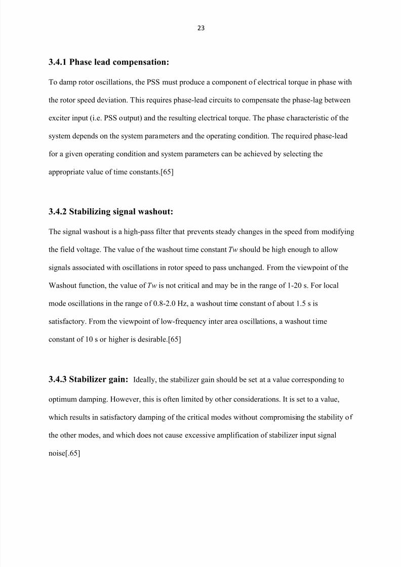
3.4.1 Phase lead compensation:

To damp rotor oscillations, the PSS must produce a component of electrical torque in phase with

the rotor speed deviation. This requires phase-lead circuits to compensate the phase-lag between

exciter input (i.e. PSS output) and the resulting electrical torque. The phase characteristic of the

system depends on the system parameters and the operating condition. The required phase-lead

for a given operating condition and system parameters can be achieved by selecting the

appropriate value of time constants.[65]

3.4.2 Stabilizing signal washout:

The signal washout is a high-pass filter that prevents steady changes in the speed from modifying

the field voltage. The value of the washout time constant T w should be high enough to allow

signals associated with oscillations in rotor speed to pass unchanged. From the viewpoint of the

Washout function, the value of T w is not critical and may be in the range of 1-20 s. For local

mode oscillations in the range of 0.8-2.0 Hz, a washout time constant of about 1.5 s is

satisfactory. From the viewpoint of low-frequency inter area oscillations, a washout time

constant of 10 s or higher is desirable.[65]

3.4.3 Stabilizer gain: Ideally, the stabilizer gain should be set at a value corresponding to

optimum damping. However, this is often limited by other considerations. It is set to a value,

which results in satisfactory damping of the critical modes without compromising the stability of

the other modes, and which does not cause excessive amplification of stabilizer input signal

noise[.65]



24

3.5 Modeling of a single machine system connected to infinite bus system:

Fig.3 A Single Machine System

consider a single machine system connected to a infinite bus system

-

+ +

Fig.4.Excitation system



25

Torque angle loop: By solving the following torque angle loop and rotor mechanical equations

we get the equations for K1 and K2 values

Fig.5.Torque angle loop

Representation of flux decay:

By solving the flux decay blocks we get the values of K3 and K4

+ -

Fig.6.Representation of flux decay



26

Representation of excitation system:

By solving the block diagram we can get the values of K5 and K6

Fig.7.Excitation system block diagram

The coefficients K1 to K6 that are obtained from the block diagrams are termed as

Heffron-Phillips constants. They are dependent on machine parameters and operating conditions

Generally K1,K2,K3 and K6 are positive. K4 is also mostly positive except for cases when Re is

high. K5 can be either positive or negative. K5 is usually negative for moderate to high external

impedances and heavy loadings. For Re=0 the expressions for the constants K1 to K6 are

simplified. As the armature resistance is already neglected, this refers to a lossless network on

the stator side.



27

The expressions are given below:

It is to be noted that Heffron-Phillips constants can also be defined for any general network

connected between the generator and infinite bus[64].



28

4. ARTIFICIAL NEURAL NETWORK

Artificial neural networks can be most adequately characterised as µcomputational models¶

with particular properties such as the ability to adapt or learn, to generalize, or to cluster or

organise data, and which operation is based on parallel processing. However, many of the

above mentioned properties can be attributed to existing (non-neural) models; the intriguing

question is to which extent the neural approach proves to be better suited for certain applications

than existing models.

An artificial network consists of a pool of simple processing units which communicate by

sending signals to each other over a large number of weighted connections.

A set of major aspects of a parallel distributed model can be distinguished by Rumelhart and

McClelland

y A set of processing units (µneurons,¶ µcells¶)

y A state of activation for every unit, which equivalent to the output of the unit.

Connections between the units. Generally each connection is defined by a weight

y This determines the effect which the signal of unit j has on unit k.

y A propagation rule, which determines the effective input of a unit from its external

Inputs.

y An activation function

, which determines the new level of activation based on the

effective input and the current activation y An external input for each unit

y A method for information gathering (the learning rule)



29

y An environment within which the system must operate, providing input signals and if

y Necessary error signals.[58]

4.1 Neuron Model:

One neuron can¶t do much on its own. Usually we will have many neurons labelled by

indices k , i, j and activation flows between them via synapses with strengths wk i, wij:

Fig.8. neuron model

An elementary neuron with R inputs is shown below. Each input is weighted with an appropriate

w. The sum of the weighted inputs and the bias forms the input to the transfer function f.

Neurons can use any differentiable transfer function f to generate their output.



30

Multilayer networks often use the log-sigmoid transfer function logsig.

The function logsig generates outputs between 0 and 1 as the neuron's net input goes from

negative to positive infinity.Alternatively, multilayer networks can use the tan-sigmoid transfer

function tansig.



31

Occasionally, the linear transfer function purelin is used in back propagation networks.

If the last layer of a multilayer network has sigmoid neurons, then the outputs of the network are

limited to a small range. If linear output neurons are used the network outputs can take on any

value.[58]

NUMBER OF LAYERS: In a feed-forward network, the inputs perform no computation and

their layer is therefore not counted. Thus a network with one input layer, n hidden layer, and one

output layer is referred to as a network with two layers. This convention is widely though not yet

universally used.



32

4.2 CHARACTERISTICS OF ARTIFICIAL NEURAL NETWORKS

y The Neural Networks exhibit mapping capabilities, that is, they can map input patterns to

their associated output patterns.

y The Neural Networks learn by examples. Thus, Neural Network architecture can be

µTrained¶ with known examples of a problem before they are tested for their µInference¶

capability on unknown instances of the problem. They can, therefore, identify new

objects previously untrained.

y The Neural Networks are robust systems and are fault tolerant. They can, therefore, recall

full patterns from incomplete, partial or noisy patterns.

y The Neural Networks possess the capability to generalize. Thus, they can predict new

outcomes from past trends.

y The Neural Networks can process information in parallel, at high speeds, and in a

distributed manner.[66]

4.3 LEARNING METHODS:

Learning of Artificial Neural Networks [58]

The most significant property of a neural network is that it can learn from environment,

and can improve its performance through learning. Learning is a process by which the free

parameters of a neural network i.e. synaptic weights and thresholds are adapted through a

continuous process of stimulation by the environment in which the network is embedded. The

network becomes more knowledgeable about environment after each iteration of learning





34

There are many different kinds of learning algorithm for example, error correction

learning, Boltzmann learning, Thorndike¶s law of effect, Hebbian learning and competitive

learning. In competitive learning the outputs of a neural network compete among themselves for

being the one to be active whereas in Hebbian learning several output neurons may be active at

the same time. Some other learning algorithms are: back propagation algorithm, conjugate

gradient descent, Quasi-Newton, Levenberg-Marquardt, quick propagation, Delta-bar-Delta, and

Kohonen training. Back propagation algorithm is the mostly used algorithm for feed-forward

neural network. It is a supervised learning algorithm, which requires a set of training data with

known input and output vector. It uses steepest gradient descent of error, which propagates

backwards for updating the synaptic weights and thresholds. The advantage of this algorithm is

the simplicity of calculation during weight updates. Although widely used, the back propagation

algorithm suffers from slow rate of convergence and hence requires long training time for large

network with large number of training patterns. However, some methods have been developed to

overcome the slow rate of learning, for example, optimization of initial weights [59], adaptation

of learning rate using delta-bar-delta learning rule [60], use of multiple activation functions [58].

Also adding a momentum factor, it can learn faster and can overcome local minima [61].

Conjugate gradient descent works by constructing a series of line searches across the

error surface. It first works out the direction of steepest descent, just as back propagation would

do. However, instead of taking a step proportional to a learning rate, conjugate gradient descent

projects a straight line in that direction and then locates a minimum along this line, a process that

is quite fast as it only involves searching in one dimension. Subsequently, further line searches

are conducted. The directions of the line searches (the conjugate directions) are chosen to try to

ensure that the directions that have already been minimized stay minimized. Quasi-Newton is the



35

most popular algorithm in nonlinear optimization, with a reputation for fast convergence. It

works by exploiting the observation that, on a quadratic error surface, one can step directly to the

minimum using the Newton step - a calculation involving the Hessian matrix. Main drawbacks

of this algorithm are that the Hessian matrix is difficult and expensive to calculate and Newton

step would be wrong if the error surface is non-quadratic. It requires a huge memory and

therefore it is not advised to use it for large networks.

Error-Correction Rules [57]

In the supervised learning paradigm, the network is given a desired output for each input

pattern. During the learning process, the actual output y generated by the network may not equal

the desired output d. The basic principle of error-correction learning rules is to use the error

signal (d -y) to modify the connection weights to gradually reduce this error. The perceptron

learning rule is based on this error-correction principle. A perceptron consists of a single neuron

with adjustable weights, w,, j = 1,2, . . . , n, and threshold u, as shown in Figure 2.2. Given an

input vector x= (x1, x2,. . . , x j), the net input to the neuron is

u xwvn

j

j j!§

!1 ««««««.. «««««23

The output y of the perceptron is + 1 if v > 0, and 0 otherwise. In a two-class

classification problem, the perceptron assigns an input pattern to one class if y = 1, and to the

other class if y=0.



36

0

1

!§!

u x w n

j

j j

«««««.1

The linear equation defines the decision boundary (a hyper plane in the n-dimensional

input space) that halves the space.

Rosenblatt developed a learning procedure to determine the weights and threshold in a

perceptron, given a set of training patterns. Note that learning occurs only when the perceptron

makes an error. Rosenblatt proved that when training patterns are drawn from two linearly

separable classes, the perceptron learning procedure converges after a finite number of iterations.

This is the perceptron convergence theorem. In practice, you do not know whether the patterns

are linearly separable. Many variations of this learning algorithm have been proposed in the

literature. Other activation functions that lead to different learning characteristics can also be

used. However, a single-layer perceptron can only separate linearly separable patterns as long as

a monotonic activation function is used. The back-propagation learning algorithm is also based

on the error-correction principle.

4.4 BACKPROPAGATION:

Backpropagation is the generalization of the Widrow-Hoff learning rule to multiple-layer

networks and nonlinear differentiable transfer functions. Input vectors and the corresponding

target vectors are used to train a network until it can approximate a function, associate input

vectors with specific output vectors, or classify input vectors in an appropriate way. Networks



37

with biases, a sigmoid layer, and a linear output layer are capable of approximating any function

with a finite number of discontinuities.

Standard backpropagation is a gradient descent algorithm, as is the Widrow-Hoff

learning rule, in which the network weights are moved along the negative of the gradient of the

performance function. The term backpropagation refers to the manner in which the gradient is

computed for nonlinear multilayer networks. There are a number of variations on the basic

algorithm that are based on other standard optimization techniques, such as conjugate gradient

and Newton methods.

Properly trained backpropagation networks tend to give reasonable answers when

presented with inputs that they have never seen. Typically, a new input leads to an output similar

to the correct output for input vectors used in training that are similar to the new input being

presented. This generalization property makes it possible to train a network on a representative

set of input/target pairs and get good results without training the network on all possible

input/output pairs.

There are generally four steps in the training process:

1. Assemble the training data.

2. Create the network object.

3. Train the network.

4. Simulate the network response to new inputs.



38

In back propagation it is important to be able to calculate the derivatives of any

transfer functions used. Each of the transfer functions above, logsig, tansig, and purelin, can be

called to calculate its own derivative. The three transfer functions described here are the most

commonly used transfer functions for back propagation, but other differentiable transfer

functions can be created and used with back propagation if desired.

4.4.1 FEED FORWARD NETWORK

where the data flow from input to output units is strictly feed-forward. The data processing can

extend over multiple (layers of) units, but no feedback connections are present, that is,

connections extending from outputs of units to inputs of units in the same layer or previous

layers.A single-layer network of S logsig neurons having R inputs is shown below in full detail

on the left and with a layer diagram on the right.

Feedforward networks often have one or more hidden layers of sigmoid neurons followed by an

output layer of linear neurons. Multiple layers of neurons with nonlinear transfer functions allow



39

the network to learn nonlinear and linear relationships between input and output vectors. The

linear output layer lets the network produce values outside the range -1 to +1.

On the other hand, to constrain the outputs of a network (such as between 0 and 1), then

the output layer should use a sigmoid transfer function (such as logsig).

As noted in Neuron Model and Network Architectures, for multiple-layer networks the

number of layers determines the superscript on the weight matrices. The appropriate notation is

used in the two-layer tansig/purelin network shown next.

This network can be used as a general function approximator. It can approximate any

function with a finite number of discontinuities arbitrarily well, given sufficient neurons in the

hidden layer.

4.4.2 RECURRENT NETWORKS that do contain feedback connections. Contrary to feed-

forward networks, the dynamical properties of the network are important. In some cases, the

activation values of the units undergo a relaxation process such that the network will evolve to a



40

stable state in which these activations do not change anymore. In other applications, the change

of the activation values of the output neurons are significant such that the dynamical behaviour

constitutes the output of the network.

4.4.3 Levenberg-Marquardt algorithm

The Levenberg-Marquardt algorithm was designed to approach second-order training

speed without having to compute the Hessian matrix. When the performance function has the

form of a sum of squares (as is typical in training feed forward networks), then the Hessian

matrix can be approximated as

««««««««.2

and the gradient can be computed as

««««««««.3

where J is the Jacobian matrix that contains first derivatives of the network errors with respect to

the weights and biases, and e is a vector of network errors. The Jacobian matrix can be computed

through a standard backpropagation technique that is much less complex than computing the

Hessian matrix.

The Levenberg-Marquardt algorithm uses this approximation to the Hessian matrix in the

following Newton-like update:



41

«««««««.4

When the scalar is zero, this is just Newton's method, using the approximate Hessian matrix.

When is large, this becomes gradient descent with a small step size. Newton's method is faster

and more accurate near an error minimum, so the aim is to shift toward Newton's method as

quickly as possible. Thus, is decreased after each successful step (reduction in performance

function) and is increased only when a tentative step would increase the performance function. In

this way, the performance function is always reduced at each iteration of the algorithm.

4.5 BACKPROPAGATION LEARNING ALGORITHM

There are many variations of the backpropagation algorithm. The simplest

implementation of backpropagation learning updates the network weights and biases in the

direction in which the performance function decreases most rapidly, the negative of the gradient.

One iteration of this algorithm can be written[66]

«««««««..5

where is a vector of current weights and biases, is the current gradient, is the

learning rate.

There are two different ways in which this gradient descent algorithm can be

implemented: incremental mode and batch mode. In incremental mode, the gradient is computed



42

and the weights are updated after each input is applied to the network. In batch mode, all the

inputs are applied to the network before the weights are updated.[66]

ALGORITHM:

Step 1: Normalise the inputs and outputs with respect to their maximum values. It is proved that

the neural networks work better if inputs and outputs lie between 0 and 1. For each training

pair,assume there are µl¶ inputs given by { I } l*1 and µn¶ outputs {O}n*1 in a normalised form.

Step 2:Assume the number in the hidden layer to lie between l<m<2l

Step 3:[V] represents the weights of synapses connecting input neurons and hidden neurons and

[W] represents weights of synapses connecting hidden neurons and output neurons. Initialise the

weights to small random values usually from -1 to 1. For general problems, can be assumed as

1 and the threshold values can be taken as zero.

= [random weights]

= [random weights]

= «««««6

Step 4: For the training data, present one set of inputs and outputs. Present the pattern to the

input layer as inputs to the input layer. By using linear activation function, the output of the

input layer may be evaluated as

««««««««««7



43

Step 5: Compute the inputs to the hidden layer by multiplying corresponding weights of

synapses as

««««««8

Step 6: Let the hidden layer units evaluate the output using the sigmoidal function as

............................9

Step 7: Compute the inputs to the output layer by multiplying corresponding weights of synapses

as

««««««..10

Step 8: Let the output layer units evaluate the output using sigmoidal function as

«««««««..11

Step 9: Calculate the error and the difference between the network output and the desired output

as for the ith training set as

««««««««..12

Step 10: Find {d} as

«««««««««13



44

Step 11: Find [Y] matrix ase

[Y]=««««««««..14

Step 12: Find

«««««««..15

Step 13: Find {e}= [W] {d}

«««««««««.16

Find [X] matrix as

[X]= «««««««.17

Step 14: Find =

Step 15: Find

««««««««««18

««««««««..19

Step 16: Find error rate as

Error rate =

««««««««..20

Step 17: Repeat steps 4-16 until the convergence in the error rate is less than the tolerance value.



45

5. MATHEMATICAL MODELLING

The system equations are non linear and have to be solved numerically. in solving these

equations it is assumed that the system][ is at stable equilibrium point till time t=0 and

disturbance occurs at t=0 or later. From the power flow calculations in the steady state,we get the

real and reactive power(Pt and Qt),the voltage magnitude (Vt )and angle() at the generator

terminals. Here is the angle w.r.t to the slack bus[64]

Step1 : T o find Heffron- P hillips constants :

««««««««««««««21

j ««««««««««««22

If

Then

««««««««««««««.23

Else =

«««««««««««««««..24

«««««««««««.....25

«««««««««««««....26

««««««««««««««27

««««««««««««««28



46

««««««««««««««...29

««««««««30

«««««««««««««««««««31

««««««««««««««««««..32

«««««««««««««««33

««««««««.......34

«««««««««««««««..35



47

Step2 : To find matrices A, B and C.

A= [ 0 wo 0 0

/(2h) 0 (-/(2h)) 0

- /(2h) 0 (-/()) (1/)

(-)/ 0 (-)/ -(1/) ]

=

C=

Step3 : F or finding eigen vectors [55]

««««««««..36

Selection of is to be done

For system to be stable the real part of should be negative.

Assume

If imaginary part of

««««««««««««..37



48

Else

««««..38

Now + j (imaginary part of ««««.39

Step4 : T o find values [55]

««««««40

««.41

«««««««««.42



49

6.Experimental investigations

From the mathematical modelling,for different P and Q values Heffron-Phillip constants(K1-K6)

are calculated. Using state variable method the values for stabilizer gain (Kstab) and time

constant (T1) are calculated . The following are the values obtained shown in table 1

P (p.u) Q (p.u) K1 K2 K3 K4 K5 K6 Kstab T1

0.7 -0.5 1.0308 1.3845 0.3600 1.7722 -0.1516 0.1128 18.4242 0.1318

1 0 1.1060 1.3288 0.3600 1.7009 -0.1002 0.3608 36.9937 0.0534

1 0.5 1.1718 1.2557 0.3600 1.6073 -0.0793 0.4185 43.4259 0.0470

0.8 -0.2 1.0789 1.3659 0.3600 1.7484 -0.0868 0.2701 27.7016 0.0667

0.6 -0.3 1.0701 1.3349 0.3600 1.7087 -0.2280 0.2770 23.9444 0.0597

0.9 -0.4 0.9821 1.3816 0.3600 1.7685 -0.1945 0.1460 23.5048 0.1115

Table 1: Pss parameters and Heffron-Phillip constants calculated through off line studies

By substituting the values of (K1-K6) and Kstab and T1 in the following figures and

simulation is done and the obtained deviation plots are observed.

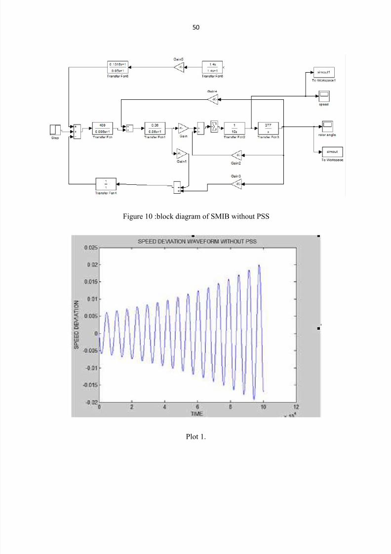
Figure .10 shows the block diagram of SMIB without PSS and the figure 11. Shows

the block diagram of SMIB with PSS and the plot 1, plot 2 show speed deviation waveform and

rotor angle deviation waveform without PSS respectively. The plot 3, plot 4 show speed

deviation waveform and rotor angle deviation waveform with PSS respectively



50

Figure 10 :block diagram of SMIB without PSS

Plot 1.



51

Plot 2.

Figure 11 :block diagram of SMIB with PSS



52

Plot 3.

Plot 4.

Now an artificial neural network is introduced to make a conventional PSS to a self ±tuning

ANNPSS. The figure 12. Shows how an ANN is connected to the PSS



53

Figure 12.

Figure 13. simulated block diagram of ST-ANNPSS



54

The following plots are obtained for different values of P and Q for conventional power system

stabilizer(CPSS) and self-tuning power system stabilizer using artificial neural network(ST-

ANNPSS)

Plot.5

Plot.6



55

Plot.7

Plot.8



56

Plot.9

Plot.10



57

Plot.11

Plot.12



58

Performance plots of neural network for different number of neurons in hidden layer

30 neurons ; Time:27 secs ; Iterations:1000

Plot .13

40 neurons ; Time:11 secs ; Iterations:272

Plot.14



59

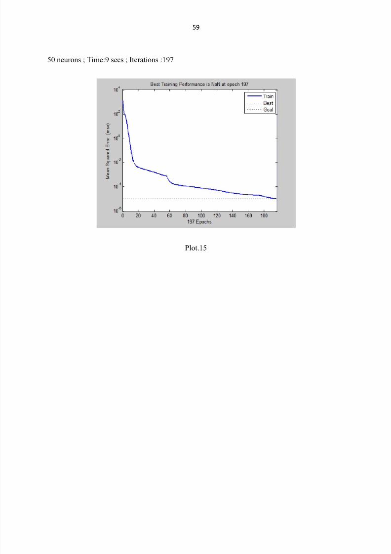
50 neurons ; Time:9 secs ; Iterations :197

Plot.15



60

7.Experiments results

Table.2 operating conditions and optimum PSS parameters computed through off-line studies

Table.3 PSS parameters computed using ANN for 40 neurons and 50 neurons



61

8.Discussions of experimental results and experimental investigations:

y When figure .10 is simulated plots.1 and plot .2 are observed and the speed deviation

waveform and rotor angle deviation waveform and it can seen that system is not stable.

y When figure 11 is simulated plots 3 and 4 are observed and speed,rotor angle deviation

waveform reach steady state, meaning that system is stable with PSS

y When figure13 is simulated and is compared with conventional PSS plots 5,6 are

obtained for P=0.7,Q=-0.5 and we can observe that the waveform match with each

other to great extent.

y When P and Q values are changed the usage of ANN makes the system to settle with less

number of oscillations compare to CPSS as shown in plots 7,8,9,10,11,12.

y Performance of the ANN is observed for different number the ANN is observed for

different number of neurons in the hidden layer and performance graphs are observed

for 30,40,50 neurons .

y For 30 neurons the performance goal is not reached even for 1000 iterations

y For 40 neurons the goal is reached for 272 iterations in 11 seconds and the gain values

are near to the off line studies

y For 50 neurons the goal is reached in 197 iterations is 9seconds

y Number of iterations per second for 40 neurons=24.72

And

y Number of iterations per second for 50 neurons=21.88

So from above it can be seen that the suitable value for number of neurons is 40.



62

9.CONCLUSIONS

Chapter 3 describes the need of the power system stabilizers and the problem of

the low frequency oscillations (0.2 Hz to 3.0 Hz), which limit the power transmission capability

of a network and, sometimes, even cause a loss of synchronism and an eventual breakdown of

the entire system. The application of Power System Stabilizer (PSS) can help in damping out

these oscillations and improve the system stability. The literature survey shows the interest of

adaptive PSS and in that way ANN is very helpful for robust design of PSS.

In chapter 4, ANN over view , the error-correction rules and Back-propagation algorithm

are given which are very helpful for design of ANNPSS .

In chapter 6 an artificial neural network has been developed for the tuning of power

system stabilizers. The ANN receives generator real power(P) and reactive power(Q), which

characterize the loading condition of a generator, as its inputs and provides the desired PSS

parameter settings as its output. In the training process, several input-output training patterns are

first compiled .These training patterns are used to train the neural network and obtain the

connection weights between neurons. Once trained, the ANN is capable of providing the PSS

parameters in real-time based on on-line measured system operating point.

In chapters 6 and 7, studies shows that dynamic performance with self-tuning PSS is

virtually identical to that obtained with conventional PSS at nominal operating point. However,

the dynamic performance of self-tuning ANNPSS is quite superior to that of conventional PSS

for the loading condition different from the nominal. Investigations also reveal that the

performance of self-tuning ANNPSS is quite robust to a wide variation in loading condition.

Simulation results for a synchronous generator subject to a severe change in the operating



63

condition indicate that, when the parameter settings are updated in real-time by the ANN, the

PSS can offer good dynamic performance over a wide range of operating conditions. On the

other hand, a PSS with fixed parameter settings can only provide good damping effect under

some particular operating points. Since the proposed ANN approach does not require model

identification in deriving the PSS parameters, it is more efficient than the self-tuning controllers

and is, therefore, more suitable for real-time applications.



64

10.REFERENCES

[1] F. P. Demello and C. Concordia , Concepts of Synchronous Machine Stability as Effected by

Excitation Control", IEEE Transactions on Power Apparatus and Systems, Vol. PAS-88, No. 4, pp.

316-329, April 1969.

[2] A. Klofenstein, Experience with System Stabilizing Excitation Controls on the Generation of the

Southern California Edition Company", IEEE Transactions on PAS, Vol. 90, No. 2, pp. 698-706,

March/April 1971.

[3] IEEE Working Group Annotated Bibliography on Power System Stability Controls 1986- 1994 ",

IEEE Transactions on Power Systems, Vol. 88, No. 4, pp. 794-804, May 1996.

[4] K. Bollinger, A. Laha, R. Hamilton and T. Harras, Power System Stabilizer Design Using Root-

Locus Methods", IEEE Transaction on PAS, Vol. 94, No. 5, pp. 1484-1488, Sep/Oct. 1975.

[5] F.P. Demello, P.J. Nolan, T.F. Laskowski, and J.M. Undrill, Coordinated Application of Stabilizers

in Multi-machine power systems", IEEE Transactions on PAS, Vol. 99, pp. 892-901, 1980.

[6] R.V. Larsen and D.A. Swann, Applying Power System Stabilizers, I, II and III", IEEE Transactions

on PAS, Vol. 100, No.6, pp. 3017-3046, June 1981.

[7] J.S. Czuba, L.N. Hannett and J.R. Willis, Implementation of Power System Stabilizer at the

Ludington Pumped Storage Plant", IEEE Transactions on Power Systems, Vol. PWRS-1, pp. 121-

128, Feb. 1986.

[8] C.T. Tse, S.K. Tso, Approach to the Study of Small-perturbation Stability of Multi- machine

Systems ", IEE Proceedings, Generation, Transmission and Distribution, Vol. 135, No. 5, pp. 396-

405, 1988.

[9] C. Chen, Y. Hsu, Coordinated Synthesis of Multi-machine Power System Stabilizers Using an

Efficient Decentralized Modal Control Algorithm", IEEE Transactions on Power Systems, Vol. 2,

No. 3, pp. 543-551, Aug. 1987.

[10] C.T. Tse, S.K. Tso, Refinement of Conventional PSS Design in Multi-machine System by Modal

Analysis", IEEE Transactions on Power Systems, Vol. 8, No. 2, pp. 598-605, May 1993.

[11] Yao-Nan Yu and Qing-Hua Li, Pole Placement Power System Stabilizers Design of an Unstable

Nine-Machine System", IEEE Transactions on PAS, Vol. 5, No. 2, May 1990.

[12] Y.N. Yu, K.Vongsuriya, and I.N. Wedman, Application of an Optimal Control Theory to a Power

System", IEEE Transactions on PAS, Vol. 89, No. 1, pp 55-61, 1970.

[13] Y. Lee and C. Wu , Damping of Power System Oscillations With Output Feedback and Strip

Eigenvalue assignment ", IEEE Transactions on Power Systems, Vol. 10, No. 3, pp 1620-1626,

Aug 1995.



65

[14] M.R. Khaldi, A.K. Sarkar, K.Y. Lee, and Y.M. Park , The Modal Performance Measure for

Parameter Optimization of Power System Stabilizers", IEEE Transactions on Energy Conversion,

Vol. 8, No. 4, pp 660-666, Dec 1993.

[15] J.B. Simo, I. Kamwa, G. Trudel, and S. Tahan, Validation of a New Modal Performance Measurefor Flexible Controllers Design", IEEE Transactions on Power Systems, Vol. 11, No. 2, pp 819-

826, May 1996.

[16] A.J. Urdaneta, N.J. Bacalao, B. Feijoo, L. Flores, and R. Diaz, Tuning of Power System Stabilizers

Using Optimization Techniques", IEEE Transactions on Power Systems, Vol. 6, No. 1, pp 127-134,

Feb. 1991.

[17] Jan Lunze, Robust Multivariable Feedback Control", Prentice Hall International, U.K., 1989.

[18] D.A. Pierre, A Perspective on Adaptive Control of Power Systems", IEEE Transactions on PWRS,

Vol. 2, No. 2, pp. 387-396, May 1987.[19] A. Ghosh, G. Ledwich, O.P. Malik and G.S. Hope, Power System Stabilizer Based on Adaptive

Control Techniques", IEEE Transactions on PAS, Vol. 103, pp. 1983-1989, March/April 1984.

[20] O.P. Malik, G.S. Hope and Ramanujan, Real Time Model Reference Adaptive Control of

Synchronous Machine Excitation", IEEE PES Winter Meeting Paper, 178, 297-304, 1976.

[21] A. Ghandakly and P. Idowu, Design of a Model Reference Adaptive Stabilizer for the Exciter and

Governor Loops of Power Generators", IEEE Transactions on PAS, Vol. 5, pp. 887-893,

March/April 1990.

[22] Shi-Jie Cheng, O.P. Malik and G.S. Hope, Self Tuning Stabilizer for a Multi-machine Power System", IEE Proceedings, Part C, No. 4, pp. 176-185, 1986.

[23] A. Chandra, O.P. Malik and G.S. Hope A self-Tuning Controller for the Control of Multi-mahine

Power Systems", IEEE Transactions on PAS, Vol. 3, No. 3, pp. 1065-1071, Aug. 1988.

[24] N.C. Pahalawaththa, G.S. Hope and O.P. Malik, Multivariable Self-Tuning Power System

Stabilizer Simulation and Implementation Studies", IEEE Transactions on Energy Conversion, Vol.

EC-6, No. 2, pp. 310-316, June 1991.

[25] F. Ghosh and Indraneel Sen, Design and Performance of a Local Gain Scheduling Power System

Stabilizer for Interconnected System", TENCON-91, International Conference on EC3-Energy,Computer, Communication and Control Systems, Vol. 1, pp. 355-359, Aug. 1991.

[26] D.P. Sen Gupta, N.G. Narhari, I. Boyd and B.W. Hogg, An Adaptive Power System Stabilizer

which Cancels the Negative Damping Torque of a Synchronous Generator", Proceedings of IEE,

Part. C, pp. 109-117, 1985.





67

[42] António C. Andrade ,F. P. Maciel Barbosa, J. N. Fidalgo and J. Rui Ferreira´ Voltage stability

Assessment Using a New FSQV Method and Artificial Neural Networks´ IEEE MELECON 2006,

May 16-19, Benalmádena (Málaga), Spain.

[43] Antonio C. Andrade, F. P. Maciel Barbosa,´ FSQV and Artificial Neural Networks toVoltage Stability Assessment´.

[44] S. Chauhan and M.P. Dave, ³Sensitivity based voltage instability alleviation using ANN´ IEEE

Transactions on Electrical Power and Energy Systems 25 (2003) 651±657

[45] H .P. Schmidt,´ Application of artificial neural networks to the dynamic analysis of the voltage

stability problem´, IEE proc.-gener.transm.distrib.Vol.144,No.4 , July 1997

[46] B. Jeyasurya,´ Artificial Neural Networks For on-line Voltage stability Assessment´ 0-7803-6420-

1/00/$10.00 (c) 2000 IEEE

[47] Y. Zhang and Z. Zhou, ³Online Voltage Stability Contingency Selection Using Improved RSIMethod Based on ANN Solution´ 0-7803-7322-7/02/$17.00 © 2002 IEEE

[48] Bansilall, D. Thukaram', and K. Harish Kashyap', Artificial Neural Network Application to Power

System . Voltage Stability Improvement ³0-7803-7651-x/03~17.000 2 003 lEEE

[49] S. Kamalasadan, , A. K. Srivastava, and D. Thukaram,³Novel Algorithm for Online voltage

Stability Assessment Based on Feed Forward Neural Network´ 1-4244-0493- /06/$20.00 ©2006

IEEE.

[50] Mohamed M. Hamada, Mohamed A. A. Wahab and Nasser G. A. Hemdan, ³Artificilal Neural

Network Modeling Technique for Voltage Assessment of Radial Disribution Systems´[51] S.Sahari, A.F.Abidin, and T.K.Abdul Rahman,´Development of Artificial Neural network for

Voltage Stability Monitoring´,National Power and Energy conference(PECon)2003

Proceedings,Bangi, Malaysia.

[52] Hsu Y-Y, Chen C-R. "Tuning of power system stabilizers using an artificial neural network". IEEE

Trans Energy Conversion 1991 ; 6(4):612-9.

[53] Zhang Y, Chen GP, Malik OP, Hope GS. An artificial neural network based adaptive power system

stabilizer. IEEE Trans Energy Conversion 1993;8(1):71-7.

[54] Zhang Y, Malik OP, Chen GP. Artificial neural network power system stabilizers in multi-machine power system environment. IEEE Trans Energy Conversion 1995;10(1):147-54.

[55] Guan L, Cheng S, Zhou R., Artificial neural network power system stabilizer trained with an

improved BP algorithm. IEE Proceedings on Generation Transmission Distribution 1996;

143(2):135-141.



68

[56] Park YM, Lee KY, A neural network based power system stabilizer using power flow

characteristics. IEEE Trans Energy Conversion 1996;11(2):435-41.

[57] Ani1 K. Jain ,Jianchang Mao and K.M. Mohiuddin "Artificial neural networks: A Tutorial"0018-

9162/96/ march 1996 IEEE, pp. 31-44.

[58] Simon Haykin, ³Neural Network: A Comprehensive Foundation´, 2nd

Edition, IEEE Press, 1999.

[59] Jim Y. F. Yam and Tommy W. S. Chow, ³Feed forward Coefficients Networks Training Speed

Enhancement by Optimal Initialization of the Synaptic´ IEEE Transactions on Neural Networks,

Volume 12, No.2, March 2001, pp.430-434.

[60] R. Haque, N. Chowdhury, ³An Artificial Neural Network Based Transmission Loss Allocation For

Bilateral Contracts´ 18th Annual Canadian Conference on Electrical and Computer Engineering

CCECE05, May 1-4, 2005, pp. 2197-2201.

[61] Phansalkar, V.V., Sastry, P.S., ³Analysis of the back-propagation algorithm with momentum´,

IEEE Transactions on Neural Networks, Volume: 5, Issue: 3, May 1994, pp. 505 ± 506.

[62] Ping Chang and Jeng-Shong Shih ,"The Application of Back Propagation Neural Network of Multi-

channel Piezoelectric Quartz Crystal Sensor for Mixed Organic Vapours" Tamkang Journal of

Science and Engineering, Vol. 5, No. 4, 2002, pp. 209 ±217.

[63] Kundur, P., Power System Stability and Control, McGraw-Hill, 1994

[64] K.R.Padiyar.,Power system dynamics stability and control., 2nd

Edition.,BS publications.

[65] Ravi Segala, Avdhesh Sharmab, M.L. Kotharic´ A self-tuning power system stabilizer

based on artificial neural network´ Received 14 November 2001; revised 3 October 2003; accepted 7

November 2003

[66] S.Rajasekaran,G.A.Vijayalakshmi Pai,´neural networks,fuzzylogic and genetic algorithms synthesis

and applications´



69

11.APPENDIX

Data used for test system

Nomenclature

h -- inertia constant

E b -- infinite bus voltage

T m , T e -- mechanical and electrical torques, respectively

X d -- direct axis reactance

f(Hz) D( pu) h( sec) Ra( pu) xd ( pu) xq( pu) Xd ' ( pu) Xq

' ( pu) T do' ( sec) T qo

' ( sec)

60 0.0 5.0 0.0 1.6 1.55 0.32 0.5 6.0 0.81

E b X e( pu) K A( sec) T A( pu) T r ( sec) T3( sec) T w( pu) T2

1 0.4 5.0 0.006 0.0 2.1 1.4 0.05



70

X q -- quadrature axis reactance

X d ' -- direct axis transient reactance

Xq' -- quadrature axis transient reactance

X l -- leakage reactance

Ra -- stator resistance per phase

E fd -- equivalent exciter voltage

D -- damping factor

T r -- terminal voltage transducer time constant

Vref -- AVR reference signal

K A,TA -- AVR gain and time constant, respectively

VS -- stabilizing signal

TW -- washout time constant

K stab -- PSS gain

T1,T2 -- PSS time constants

Xe -- equivalent resistance and reactance respectively

Documents

Full Report3