Full-Scale Testing of Enhanced Mercury Control ... Library/Research/Coal/ewr/mercury... · FULL-SCALE TESTING OF ENHANCED MERCURY CONTROL TECHNOLOGIES FOR WET FGD SYSTEMS Final Report

FULL-SCALE TESTING OF ENHANCED MERCURY CONTROL TECHNOLOGIES FOR WET FGD SYSTEMS

Final Report For the period: October 1, 2000 to June 30, 2002

Prepared by:

BABCOCK & WILCOX COMPANY

Power Generation Group 20 South Van Buren

Barberton, Ohio 44203-0351 D. K. McDonald

Phone: (330) 860-6175, Fax: (330) 860-2348

and

McDERMOTT TECHNOLOGY, INC. Research and Development Division

1562 Beeson Street Alliance, Ohio 44601-2196

G. T. Amrhein Phone: (330) 829-7747, Fax: (330) 829-7283

G. A. Kudlac Phone: (330) 829-7372, Fax: (330) 829-7283

D. Madden Yurchison Phone: (330) 829-7839, Fax: (330) 829-7283

Submitted by:

McDermott Technology, Inc. Contract Research Division

Date published: May 7, 2003 FINAL EDITION

This report does not contain any Trade Secret/Proprietary Information.

This project was funded in part by the U. S. Department of Energy and the Ohio Coal Development Office, Department of Development, State of Ohio

U.S. Department of Energy Contract: DE-FC26-00NT41006 Ohio Coal Development Office Grant Agreement: CDO/D-99-03 McDermott Technology, Inc. Contract: CRD 1427

Legal Notice/Disclaimer "This report was prepared by McDermott Technology, Inc. (MTI) pursuant to a contract partially funded by the U. S. Department of Energy (DOE) and the Ohio Coal Development Office /Ohio Department of Development (OCDO/ODOD). Neither the State of Ohio nor any of its agencies, the DOE, nor MTI, nor any of it’s subcontractors, nor any person acting on behalf of either:

(a) makes any warranty or representation, express or implied, with respect to the accuracy, completeness, or usefulness of information contained in this report, or that the use of any information, apparatus, method, or process disclosed in this report may not infringe privately owned rights; or

(b) assumes any liabilities with respect to the use of, or for damages resulting from the

use of, any information, apparatus, method or process disclosed in this report. Reference herein to any specific commercial product, process, or service by trade name, trademark, manufacturer, or otherwise, does not necessarily constitute or imply its endorsement, recommendation, or favoring nor do the view and Opinions of authors expressed herein necessarily state or reflect those of the State of Ohio nor the DOE.

NOTICE to JOURNALISTS AND PUBLISHERS: Please feel free to quote and borrow from this report, however, please include a statement noting the Ohio Coal Development Office’s support for this project.

Page i

TABLE OF CONTENTS Section Page ABSTRACT/REPORT SUMMARY 1.0 EXECUTIVE SUMMARY ....................................................................................... 10 1.1 Approach...................................................................................................................... 10 1.2 Ontario Hydro Flue Gas Sampling Results Summary ................................................. 12 1.3 Mercury in Coal Utilization By-Products Results Summary....................................... 14 1.4 Market Impact.............................................................................................................. 15 1.5 Comparison with Competing Technologies................................................................. 17 2.0 INTRODUCTION...................................................................................................... 21 2.1 Background and Objectives ......................................................................................... 21 2.2 Benefits of the B&W/MTI Enhanced Wet FGD Mercury Removal Process .............. 21 2.3 Project Sponsors........................................................................................................... 22 3.0 TECHNICAL DISCUSSION ................................................................................... 23 3.1 Process Description..................................................................................................... 23 3.2 Technical Approach .................................................................................................... 23 3.2.1 Overview........................................................................................................ 23 3.2.2 Field Operation Phases .................................................................................. 26 3.2.3 Mobile Test Pump Skid ................................................................................. 27 3.2.4 Ontario Hydro Measurements – General Methodology................................. 30 3.2.5 PS Analytical Mercury Analyzer System ...................................................... 32 3.3 Ontario Hydro Flue Gas Sampling Results................................................................. 36 3.3.1 MSCPA, Endicott Station .............................................................................. 36 3.3.1.1 MSCPA Test Plan .......................................................................... 36 3.3.1.2 Plant Operation............................................................................... 39 3.3.1.3 Parametric Test Results .................................................................. 41 3.3.1.4 Performance Verification Test Results........................................... 44 3.3.1.5 Long-Term Operation..................................................................... 48 3.3.2 Cinergy, Zimmer Station ............................................................................... 52 3.3.2.1 Test Plan ......................................................................................... 52 3.3.2.2 Plant Operation............................................................................... 53 3.3.2.3 Performance Verification Results .................................................. 55 3.3.3 Ontario Hydro Flue Gas Sampling Summary and Conclusions .................... 59 3.4 A Case for Oxidation Technologies............................................................................ 60 3.5 Mercury in Coal Utilization By-Products (CUBs)...................................................... 66 3.5.1 Conventional Chemical Analyses .................................................................. 66 3.5.1.1 Endicott Stream Sampling.............................................................. 67 3.5.1.2 Zimmer Stream Sampling .............................................................. 75 3.5.1.3 Results of Conventional Chemical Analyses ................................. 84 3.5.1.4 Coal Analyses................................................................................. 88

Page ii of 151

TABLE OF CONTENTS (Cont’d) Section Page 3.5.2 Thermal Dissociation Tests............................................................................ 92 3.5.2.1 Apparatus and Method ................................................................... 93 3.5.2.2 Preparation and Testing of Standards............................................. 97 3.5.2.3 TDT Tests of Endicott and Zimmer Samples................................. 105 3.5.2.4 TDT vs. Conventional Chemistry .................................................. 112 3.5.3 Mercury Tracking ........................................................................................ 116 3.5.4 CUBs Results and Conclusions ................................................................... 119 3.6 Quality Assurance/Quality Control........................................................................... 121 3.7 Technical Conclusions .............................................................................................. 123 3.7.1 Ontario Hydro Flue Gas Sampling Conclusions.......................................... 123 3.7.2 Mercury in Coal Utilization By-Products Conclusions ............................... 124 4.0 MARKETING/COMMERCIALIZATION DISCUSSION ................................ 126 4.1 Market Application ................................................................................................... 126 4.2 By-Product Market.................................................................................................... 133 4.3 Marketplace Acceptance........................................................................................... 134 4.4 Increased Use of Ohio Coal...................................................................................... 136 4.5 Process Economics.................................................................................................... 136 4.6 Commercialization Plan............................................................................................ 137 5.0 REFERENCES........................................................................................................ 139 APPENDIX A – PROXIMATE ANALYSES FOR ZIMMER COAL SAMPLES ......A-1 APPENDIX B – PLANT DATA ACQUISITION SYSTEM DATA ..............................B-1

LIST OF TABLES Table Page 1.1-1 Test Location Characteristics Comparison.................................................................. 11 1.3-1 Average Mercury Concentration for Major Process Streams...................................... 15 1.4-1 U.S. Coal-fired Generating Market Summary............................................................. 17 1.5-1 Costs of Mercury Removal Processes ......................................................................... 19 1.5-2 Comparison of WFGD + E-Hg vs. ACI + SDA.......................................................... 20 1.5-3 Comparison of WFGD + E-Hg vs. ACI ...................................................................... 20 3.2-1 Test Location Characteristics Comparison.................................................................. 23 3.2-2 Flue Gas Sampling Details ......................................................................................... 31 3.2-3 PS Analytical Mercury Analyzer Specifications......................................................... 33 3.3-1 Summary of Parametric Tests – Endicott.................................................................... 37 3.3-2 Summary of Plant Operating Conditions – Endicott................................................... 40

Page iii of 151

LIST OF TABLES (Cont’d) Table Page 3.3-3 Summary of Hg Speciation Results – Endicott Verification Tests ............................. 46 3.3-4 Summary of Hg Speciation Results – Endicott Long Term Tests............................... 50 3.3-5 Summary of Plant Operating Conditions – Zimmer.................................................... 54 3.3-6 Summary of Hg Speciation Results – Zimmer Verification Tests .............................. 56 3.4-1 Chloride Addition Test Conditions ............................................................................. 63 3.5-1 Process Stream Sample Preparation Techniques for Mercury Analysis ..................... 66 3.5-2 Process Stream Analytical Methods............................................................................ 67 3.5-3 Samples Collected and Analyzed from Endicott......................................................... 82 3.5-4 Samples Collected and Analyzed from Zimmer ......................................................... 83 3.5-5 Results of Mercury Analyses on CUB Samples from Endicott .................................. 84 3.5-6 Results of Mercury Analyses on CUB Samples from Zimmer ................................... 85 3.5-7 Endicott Ultimate Coal Analyses, Cl and Hg.............................................................. 89 3.5-8 Endicott Coal: Cl, Hg .................................................................................................. 90 3.5-9 Zimmer Ultimate Coal Analyses, Cl and Hg............................................................... 90 3.6-1 Analytical Quality Control Checks for Trace Metal Analysis ................................. 123 4.1-1 U.S. Coal-fired Utility Industry Scrubbed and Unscrubbed Markets ...................... 126 4.1-2 U.S. Coal-fired Generating Market Summary.......................................................... 128 4.1-3 Impact of Elemental Hg Oxidation........................................................................... 129 4.1-4 Costs of Mercury Removal Processes ...................................................................... 131 4.1-5 Comparison of WFGD + E-Hg vs. ACI + SDA....................................................... 132 4.1-6 Comparison of WFGD + E-Hg vs. ACI ................................................................... 133 4.4-1 Current Status of Ohio Coal Use and Ohio Generating Capacity ............................ 136 4.5-1 Summary of Costs for 500 MW E-Hg Process ........................................................ 137

LIST OF FIGURES Figure Page 1.2-1 Summary of Hg Speciation Results - Endicott Verification Tests........................... 12 1.2-2 Summary of Hg Speciation Results - Endicott Long Term Tests ............................ 13 1.2-3 Effect of Reagent Feed Rate on outlet Hg Concentration - Endicott ....................... 13 1.2-4 Summary of Hg Speciation Results – Zimmer Verification Tests........................... 14 3.2-1 MSCPA Endicott Station, Litchfield, Michigan ...................................................... 24 3.2-2 Cinergy’s Zimmer Station, Moscow, Ohio .............................................................. 25 3.2-3 Project Schedule ....................................................................................................... 26 3.2-4 Reagent Injection Skid ............................................................................................. 27 3.2-5 Reagent Injection Skid Equipment Schematic ......................................................... 29 3.2-6 Laboratory Trailer (Exterior).................................................................................... 31 3.2-7 Laboratory Trailer (Interior)..................................................................................... 32 3.2-8 PS Analytical Mercury Analyzer Schematic............................................................ 33 3.2-9 PS Analytical Mercury Analyzer ............................................................................. 34 3.3-1 WFGD Inlet Sampling Location – Endicott............................................................. 38 3.3-2 WFGD Outlet (Stack) Sampling Location – Endicott.............................................. 38

Page iv of 151

LIST OF FIGURES (Cont’d) Figure Page 3.3-3 Hg Speciation Summary, Parametric Tests 1 – 4..................................................... 41 3.3-4 Hg Speciation Summary, Parametric Tests 5 – 8..................................................... 42 3.3-5 Summary of WFGD Outlet Hg Speciation, Parametric Tests.................................. 43 3.3-6 Effect of Reagent Feed Rate on Outlet Hg Concentration – Endicott...................... 44 3.3-7 Summary of Hg Speciation Results - Endicott Verification Tests........................... 45 3.3-8 Outlet Oxidized and Elemental Hg Concentration vs. Inlet Oxidized Hg Concentration ........................................................................................................... 47 3.3-9 Outlet vs. Inlet Elemental Hg, Verification Tests – Endicott................................... 48 3.3-10 Summary of Hg Speciation Results - Endicott Long Term Tests ............................ 49 3.3-11 Outlet vs. Inlet Elemental Hg, Verification and Long Term Tests – Endicott......... 51 3.3-12 WFGD Inlet Sampling Location – Zimmer ............................................................. 52 3.3-13 WFGD Outlet Sampling – Zimmer .......................................................................... 55 3.3-14 Summary of Hg Speciation Results – Zimmer Verification Tests........................... 53 3.3-15 Outlet Elemental Mercury Concentration as a Function of Inlet Elemental Mercury Concentration – Pilot, Endicott, and Zimmer............................................ 58 3.3-16 Speciated Mercury Removal Performance, Baseline and w/ Reagent ..................... 59 3.4-1 Mercury Speciation for Typical Ohio Coals ............................................................ 61 3.4-2 Range of Chlorine Content for Typical Ohio Coals................................................. 61 3.4-3 Comparison of Mercury Control Scenarios ............................................................. 62 3.4-4 Impact of Chloride Addition on Mercury Speciation............................................... 64 3.4-5 Effect of SCR Catalyst on Mercury Speciation ....................................................... 65 3.5-1 Endicott Coal Sampling Device and Pulverizer Feeder Sampling Port ................... 69 3.5-2 Mercury Removal Reagent Tanker at Endicott........................................................ 69 3.5-3 ESP Hoppers at Endicott .......................................................................................... 70 3.5-4 ESP Ash Sampling at Endicott................................................................................. 70 3.5-5 Pug Mill on the Waste Ash Silo at Endicott............................................................. 71 3.5-6 Limestone Slurry Pump and Storage Tank at Endicott ............................................ 71 3.5-7 Settled Sludge in a Tank in the Water Treatment Process at Endicott..................... 72 3.5-8 Sample Point for the Water Treatment Sludge at Endicott ...................................... 72 3.5-9 Treated Water Overflow Weir at Endicott ............................................................... 73 3.5-10 WFGD Slurry Sample Tap on the Absorber Recirculating Tank at Endicott .......... 73 3.5-11 Gypsum Filter Drum at Endicott .............................................................................. 74 3.5-12 Gypsum Filter Pile at Endicott ................................................................................. 74 3.5-13 Thiosorbic Lime Slurry flowing from Storage Tanks at Zimmer ............................ 77 3.5-14 Reclaim Water Sampling in the Scrubber Building at Zimmer ............................... 77 3.5-15 ESP Hopper Layout at Zimmer ................................................................................ 78 3.5-16 ESP Ash Sampling at Zimmer ................................................................................. 78 3.5-17 Ash from the South Ash Silo being Loaded into a Tanker at Zimmer..................... 79 3.5-18 WFGD Slurry Sampling at Zimmer ......................................................................... 79 3.5-19 WFGD Slurry Fines from the Centrifuges at Zimmer ............................................. 80 3.5-20 Centrate Water from the Centrifuges at Zimmer...................................................... 80

Page v of 151

3.5-21 Gypsum Pile (left, white) and Centrifuges (center, blue) at Zimmer....................... 81 3.5-22 Mercury vs. ESP Field for Endicott and Zimmer..................................................... 87 3.5-23 Mercury in Gypsum and WFGD Slurry Solids for Endicott and Zimmer ............... 87 3.5-24 Mercury in WFGD CUB for Zimmer....................................................................... 88 3.5-25 Cl and Hg in Endicott Coal Samples........................................................................ 91 3.5-26 Cl and Hg in Zimmer Coal Samples ........................................................................ 91 3.5-27 Vapor Pressure of Hg0 and Select Hg Salts.............................................................. 92 3.5-28 Thermal Dissociation Test Apparatus ...................................................................... 93 3.5-29 TDT Heated Hose, Pyrolyzer, Control Oven, Argon Flow Meters.......................... 94 3.5-30 TDT Data Acquisition System ................................................................................. 94 3.5-31 TDT, Inserting a Sample Boat into the Control Oven.............................................. 95 3.5-32 PSA Mercury Analyzer and Preconditioner............................................................. 95 3.5-33 Hg0 Impinger ............................................................................................................ 96 3.5-34 Fines in Endicott WFGD Slurry............................................................................... 97 3.5-35 Example TDC........................................................................................................... 99 3.5-36 Blank Sample Boat................................................................................................... 100 3.5-37 Multiple TDC for the HgSO4 Standard at Various Sample Weights ....................... 100 3.5-38 TDC for the HgO Standard Year 2000..................................................................... 101 3.5-39 TDC for the HgO Standard Year 2002..................................................................... 101 3.5-40 TDC for the HgS Standard Year 2000 ..................................................................... 102 3.5-41 TDC for the HgS Standard Year 2002 ..................................................................... 102 3.5-42 TDC for the HgSO4 Standard in 2000...................................................................... 103 3.5-43 TDC for the HgSO4 Standard in 2002...................................................................... 103 3.5-44 TDC for the HgCl2 Standard in 2000 ....................................................................... 104 3.5-45 TDC for the HgCl2 Standard in 2002 ....................................................................... 104 3.5-46 TDC for Endicott Gypsum ....................................................................................... 106 3.5-47 TDC for Zimmer Gypsum........................................................................................ 107 3.5-48 TDC for Endicott ESP Ash by Field ........................................................................ 107 3.5-49 TDC for Endicott Waste Ash ................................................................................... 108 3.5-50 TDC for Endicott WFGD Slurry .............................................................................. 108 3.5-51 TDC for Zimmer WFGD Slurry............................................................................ 109 3.5-52 TDC for Endicott WFGD Slurry Fines ................................................................. 110 3.5-53 TDC for Zimmer WFGD Slurry Fines .................................................................. 111 3.5-54 TDC for Endicott Water Treatment Sludge .......................................................... 111 3.5-55 TDT vs. Conventional Chemistry for ESP and Waste Ash................................... 113 3.5-56 TDT vs. Conventional Chemistry for WFGD Slurry and Gypsum....................... 114 3.5-57 TDT vs. Conventional Chemistry for WFGD Slurry Fines .................................. 115 3.5-58 Hg Flow Schematic for Endicott ........................................................................... 117 3.5-59 Hg Flow Schematic for Zimmer............................................................................ 118 4.1-1 Wet Scrubber Market by Reagent Type ................................................................ 126

Page vi of 151

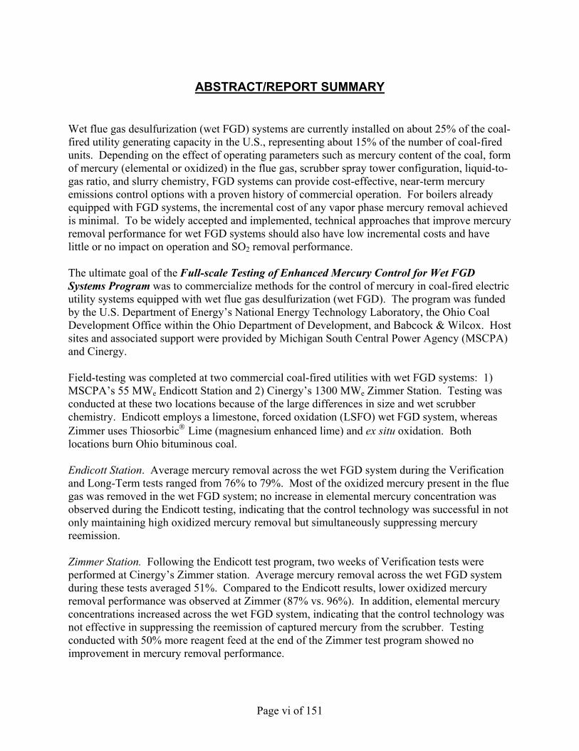
ABSTRACT/REPORT SUMMARY

Wet flue gas desulfurization (wet FGD) systems are currently installed on about 25% of the coal-fired utility generating capacity in the U.S., representing about 15% of the number of coal-fired units. Depending on the effect of operating parameters such as mercury content of the coal, form of mercury (elemental or oxidized) in the flue gas, scrubber spray tower configuration, liquid-to-gas ratio, and slurry chemistry, FGD systems can provide cost-effective, near-term mercury emissions control options with a proven history of commercial operation. For boilers already equipped with FGD systems, the incremental cost of any vapor phase mercury removal achieved is minimal. To be widely accepted and implemented, technical approaches that improve mercury removal performance for wet FGD systems should also have low incremental costs and have little or no impact on operation and SO2 removal performance. The ultimate goal of the Full-scale Testing of Enhanced Mercury Control for Wet FGD Systems Program was to commercialize methods for the control of mercury in coal-fired electric utility systems equipped with wet flue gas desulfurization (wet FGD). The program was funded by the U.S. Department of Energy’s National Energy Technology Laboratory, the Ohio Coal Development Office within the Ohio Department of Development, and Babcock & Wilcox. Host sites and associated support were provided by Michigan South Central Power Agency (MSCPA) and Cinergy. Field-testing was completed at two commercial coal-fired utilities with wet FGD systems: 1) MSCPA’s 55 MWe Endicott Station and 2) Cinergy’s 1300 MWe Zimmer Station. Testing was conducted at these two locations because of the large differences in size and wet scrubber chemistry. Endicott employs a limestone, forced oxidation (LSFO) wet FGD system, whereas Zimmer uses Thiosorbic Lime (magnesium enhanced lime) and ex situ oxidation. Both locations burn Ohio bituminous coal. Endicott Station. Average mercury removal across the wet FGD system during the Verification and Long-Term tests ranged from 76% to 79%. Most of the oxidized mercury present in the flue gas was removed in the wet FGD system; no increase in elemental mercury concentration was observed during the Endicott testing, indicating that the control technology was successful in not only maintaining high oxidized mercury removal but simultaneously suppressing mercury reemission. Zimmer Station. Following the Endicott test program, two weeks of Verification tests were performed at Cinergy’s Zimmer station. Average mercury removal across the wet FGD system during these tests averaged 51%. Compared to the Endicott results, lower oxidized mercury removal performance was observed at Zimmer (87% vs. 96%). In addition, elemental mercury concentrations increased across the wet FGD system, indicating that the control technology was not effective in suppressing the reemission of captured mercury from the scrubber. Testing conducted with 50% more reagent feed at the end of the Zimmer test program showed no improvement in mercury removal performance.

Page vii of 151

At both power plants, the wet FGD systems were very effective in removing oxidized mercury from the flue gas entering the scrubber. Total wet FGD mercury removal performance, however, was limited by the amount of elemental mercury present in the inlet flue gas. A comparison of various technical scenarios illustrated the importance of a viable mercury oxidation technology in obtaining high total wet FGD mercury removals. In one example (75% oxidized, 25% elemental entering a wet FGD system), combining a viable oxidation technology with B&W/MTI’s control technology could improve mercury removal to 91%; by comparison, either technology by itself yielded a maximum removal of 78%.

Page 10 of 151

1.0 EXECUTIVE SUMMARY A wide range of mercury emissions control performance for wet scrubbers in coal applications appear in the literature with a number of factors contributing to this variability. For example, significant differences in the mercury content of U.S. coals result in a wide range of mercury concentrations in the flue gas from the boiler. In addition, the form or species of mercury (elemental or oxidized) in the flue gas is thought to affect wet FGD system mercury removal efficiency. Mercury speciation in the flue gas is believed to be influenced by the type of coal fired, with sub-bituminous coals generating a higher relative proportion of elemental mercury than bituminous coals. Finally, the scrubber spray tower configuration, liquid-to-gas ratio, and slurry chemistry may also impact the reported mercury emissions control. Wet FGD systems are currently installed on about 25% of the coal-fired utility generating capacity in the U.S., representing about 15% of the number of coal-fired units. Depending on the effect of the operating parameters mentioned above, FGD systems can provide cost-effective, near-term mercury emissions control options with a proven history of commercial operation. For boilers already equipped with FGD systems, the incremental cost of any vapor phase mercury removal achieved is minimal. To be widely accepted and implemented, technical approaches that improve mercury removal performance for wet FGD systems should also have low incremental costs and have little or no impact on operation and SO2 removal performance. The ultimate goal of the Full-scale Testing of Enhanced Mercury Control for Wet FGD Systems Program was to commercialize methods for the control of mercury in coal-fired electric utility systems equipped with wet flue gas desulfurization (wet FGD). The two specific objectives of the project were 1) ninety percent (90%) overall system mercury removal and 2) costs below ¼ to ½ of today’s competing activated carbon mercury removal technologies. The program was funded by the U.S. Department of Energy’s National Energy Technology Laboratory, the Ohio Coal Development Office within the Ohio Department of Development, and Babcock & Wilcox. Host sites and associated support were provided by Michigan South Central Power Agency (MSCPA) and Cinergy. 1.1 APPROACH Field-testing was completed at two commercial coal-fired utilities with wet FGD systems: 1) MSCPA’s 55 MWe Endicott Station and 2) Cinergy’s 1300 MWe Zimmer Station. Testing was conducted at these two locations because of the large differences in size and wet scrubber chemistry. Endicott employs a limestone, forced oxidation (LSFO) wet FGD system, whereas Zimmer uses Thiosorbic Lime (magnesium enhanced lime) and ex situ oxidation. Both locations burn Ohio high-sulfur bituminous coal. Table 1.1-1 compares the characteristics of the two test locations.

Page 11 of 151

Table 1.1-1: Test Location Characteristics Comparison

MSCPA Endicott Station

Cinergy Zimmer Station

Electricity Generation 55 MWe 1300 MWe

Number of Wet Scrubber Modules 1 6

Wet Scrubber Reagent Limestone Thiosorbic Lime

Wet Scrubber Oxidation Method In situ Forced Oxidation

Ex situ Forced Oxidation

Wet Scrubber Liquid-to-gas Ratio 78 gal/1000 acf 21 gal/1000 acf

Slurry pH 5.4 – 5.6 5.8 – 6.0

Inlet SO2 Concentration 3600 ppm 3300 ppm

Gypsum Use Cement Wallboard Field operation began at the Endicott Station. The phases of operation at the Endicott Station were as follows:

• Parametric testing to define the optimal operating parameters for the process.

• Two weeks of verification testing to verify the performance of the process with the selected operating conditions.

• Four months of long-term operation to continue the verification of the amount of mercury

removal achieved and to prove that there were no long-term effects on SO2 removal, materials of construction, or by-product utilization.

After completing field operation at the Endicott Station, the Babcock & Wilcox / McDermott Technology Inc. (B&W/MTI) enhanced mercury removal system was moved to the Zimmer Station for testing. Field operation at the Zimmer Station included:

• Two weeks of verification testing to verify the performance of the process with the selected operating conditions. Reagent was added to all operating wet scrubbers modules simultaneously.

To facilitate minimal construction and set-up at each plant site, a mobile equipment skid was fabricated to connect to the existing wet scrubber slurry systems. Ontario Hydro measurements were made to determine total mercury and mercury speciation. Sample train and equipment preparation and recovery took place in a fully equipped, mobile laboratory trailer. The specific sampling locations for the project were the wet scrubber inlet and wet scrubber outlet (or stack). A PSA Analytical on-line mercury analyzer was also used during testing.

Page 12 of 151

1.2 ONTARIO HYDRO FLUE GAS SAMPLING RESULTS SUMMARY Endicott Station. Average mercury removal across the wet FGD system during the Verification and Long-Term tests ranged from 76% (Figure 1.2-1) to 79% (Figure 1.2-2) respectively. Most of the oxidized mercury present in the flue gas was removed in the wet FGD system; no increase in elemental mercury concentration was observed during the Endicott testing, indicating that the control technology was successful in not only maintaining high oxidized mercury removal but simultaneously suppressing mercury reemission. A general trend of decreasing mercury concentration with increasing reagent feed rate was seen as shown in Figure 1.2-3. Zimmer Station. Following the Endicott test program, two weeks of Verification tests were performed at Cinergy’s Zimmer station. Average mercury removal across the wet FGD system during these tests averaged 51% (Figure 1.2-4). Compared to the Endicott results, lower oxidized mercury removal performance was observed at Zimmer (87% vs. 96%). In addition, elemental mercury concentrations increased across the wet FGD system, indicating that the control technology was not effective in suppressing the reemission of captured mercury from the scrubber. Testing conducted with 50% more reagent feed at the end of the Zimmer test program showed no improvement in mercury removal performance.

Figure 1.2-1: Summary of Hg Speciation Results – Endicott Verification Tests (first bar of each test ID is inlet, second is outlet)

0.0

5.0

10.0

15.0

20.0

25.0

30.0

9 10 11 12 13 14 15 16 17 18 19 20 21 22

Test ID

Gas

Pha

se H

g, µ

g/ds

cm

Oxidized ElementalAvg. Removal = 76%

Page 13 of 151

Figure 1.2-2: Summary of Hg Speciation Results – Endicott Long-Term Tests

Figure 1.2-3: Effect of Reagent Feed Rate on Outlet Hg Concentration - Endicott

0

1

2

3

4

5

6

7

0 0.5 1 1.5 2 2.5 3 3.5

Reagent Feed Rate, gph

Tot

al O

utle

t Gas

Pha

se H

g, µ

g/ds

cm

0.0

5.0

10.0

15.0

20.0

25.0

30.0

35.0

24 25 26 27 28 29

Test ID

Gas

Pha

se H

g C

once

ntra

tion,

µg/

dscm

Oxidized Elemental

78% 83% 81%77%

77% 79%

Average Removal: 79%

Page 14 of 151

At both power plants, the wet FGD systems were very effective in removing oxidized mercury from the flue gas entering the scrubber. Total wet FGD mercury removal performance, however, was limited by the amount of elemental mercury present in the inlet flue gas. A comparison of various technical scenarios illustrated the importance of a viable mercury oxidation technology in obtaining high total wet FGD mercury removals. In one example (75% oxidized, 25% elemental entering a wet FGD system), combining a viable oxidation technology with B&W/MTI’s control technology could improve mercury removal to 91%; by comparison, either technology by itself yielded a maximum removal of 78%. 1.3 MERCURY IN COAL UTILIZATION BY-PRODUCTS RESULTS SUMMARY One of the most significant findings of the demonstration is that the mercury in the wet FGD Slurry was associated with the fines. This is significant because the two plants represent opposite ends of the spectrum in plant size and wet scrubber chemistry, and yet both exhibited this behavior, as did the MTI Pilot in previous studies1. It is also important because the fines can be separated from the larger gypsum crystals, through the addition of a variety of commercially available equipment, to produce a gypsum product similar to natural gypsum as shown in the table below. The fines can be disposed of in standard landfills because the mercury has been shown to be stable. This finding also suggests that the mercury in wet FGD Coal Utilization By-products (CUB) is not bound to gypsum and may be forming a fine particulate of a pure compound or reacting with some component of the fines, like soot.

0

5

10

15

20

25

30

35

40

31 32 33 34 35 36 37 38 39 40 41 42 43

Test ID

Gas

Pha

se H

g, µ

g/ds

cm

Oxidized ElementalA

vg.B

asel

ine

1130

MW

820

MW

Day

afte

r un

it tr

ip

820

MW

Figure 1.2-4: Summary of Hg Speciation Results – Zimmer Verification Tests

Page 15 of 151

Average Zimmer Endicott Natural Gypsum FGD Gypsum (w/o fines) (with fines) Minimum: 0.006 ppm (by wt) 0.03 0.03 0.48 Maximum: 0.05 ppm 1.32 0.10 1.15 From EPRI Technical Report2 TR-103652 Table 1.3-1 shows the averaged mercury concentrations for the major process streams. The important differences include the low mercury content in the Zimmer ESP Ash and Gypsum. The low mercury in the ash may be due to the low amount of unburned carbon in the Zimmer Ash (1%) compared to Endicott Ash (9%). The gypsum has low mercury because the mercury containing fines are separated from the larger gypsum crystals as part of ex situ oxidation process. The fines are not separated at Endicott, so to obtain the value shown below, the fines were separated in the lab. The mercury (and chlorine) in the coal varied by about a factor of three over the course of the test at both sites.

Table 1.3-1: Average Mercury Concentration for Major Process Streams Hg, ppm(dry) Endicott Zimmer

Coal 0.21 0.15 ESP Ash 0.32 0.016 Gypsum 0.70 0.055

Wet FGD Slurry 0.76 0.49 Wet FGD Slurry Fines 38 (by TDT) 13.3

The Thermal Dissociation Test (TDT) method was developed by MTI using the PSA Analytical mercury analyzer and appears to be a viable way of detecting small amounts of mercury in coal utilization by-products. The method produced distinct concentration vs. temperature curves for several pure mercury compounds that correlate well to vapor pressure data for these compounds. However, the curves for HgS and HgO overlap each other which make them indistinguishable. The area under the dissociation curve was shown to be directly proportional to the mercury concentration measured by conventional chemical analysis. 1.4 MARKET IMPACT In Table 1.4-1, a summary of the current U.S. coal-fired utility market is shown. The market is arranged by geographic location, coal type, FGD type (if applicable), and particulate control device (PCD). The categorical breakdowns are based on EPA-supplied data available from their website. The six highlighted rows correspond to the six largest categories within the U.S. utility market and represent 85% of the total generating capacity. The various Hg removal impact scenario calculations in the following discussion are based only on these six categories. Three Hg removal impact scenarios are shown in the table and represent the following:

Page 16 of 151

• Current: The amount of mercury removal currently achieved for the various categories with existing pollution control equipment.

• Enhanced w/o Oxidation: The amount of mercury removal possible with the application

of B&W/MTI’s wet FGD control technology to units currently equipped with wet FGD systems (activated carbon injection (ACI) control is assumed for unscrubbed units).

• Enhanced w/ Oxidation: The amount of mercury removal possible with the application

of the control technologies mentioned above plus the application of a technology capable of oxidizing 80% of the elemental mercury present in the flue gas. This technology would be applied upstream of any pollution control equipment or any mercury control technology.

For each of the three scenarios, a weighted removal average (and corresponding estimated emission rate) is calculated based on the installed generating capacity for each of the included categories. For example, the “Current” weighted removal average is 35% resulting in an estimated emission rate of 54 tons Hg/year, which agrees well with the generally reported rate of 50 to 55 tons Hg/year. The scenarios also assume that no fuel switching occurs. The results presented in Table 1.4-1 illustrate several key considerations for improving Hg removal performance for coal-fired utilities:

• Two-thirds of the current U.S. generating capacity is supplied by ESP-equipped bituminous-fired and ESP-equipped sub-bituminous-fired units. Improved Hg control for these units will have a major impact on the nationwide emissions rate.

• Applying B&W/MTI’s enhancement technologies to both scrubbed and unscrubbed

units results in a 50% decrease in the emissions rate, from 54 tons/yr to 27 tons/yr.

• Combining B&W/MTI’s control technologies with an oxidation technology capable of oxidizing 80% of the elemental Hg present in the flue gas results in a further reduction of 50%, down to 14 tons/yr. This reduction is due primarily to the conversion (and capture) of the significant amount of elemental mercury generated by the sub-bituminous-fired units.

• Even with the high levels of oxidized mercury generated in the oxidation-based

scenario, ACI injection removes less Hg than wet scrubbing.

Page 17 of 151

Table 1.4-1: U.S. Coal-fired Generating Market Summary

Hg Removal Impact Scenarios

Location Coal Type

FGD Type

PCD Type MW

% of Total MW

Current Enhanced w/o Hg°

Oxidation

Enhanced w/ Hg°

Oxidation Scrubbed Units East Bit Wet ESP 39,345 12.8 63% 80% 92% East Bit Wet Other 3,496 1.1 East Bit Dry ESP 160 0.1 East Bit Dry Other 3,017 1.0 East Sub Wet ESP 1,954 0.6 East Sub Wet Other 44 0.0 West Bit Wet ESP 2,305 0.8 West Bit Wet Other 1,498 0.5 West Bit Dry Other 1,256 0.4 West Sub Wet ESP 13,412 4.4 57% 72% 91% West Sub Wet Other 9,867 3.2 57% 72% 91% West Sub Dry ESP 1,562 0.5 West Sub Dry Other 4,588 1.5 West Lig Wet ESP 8,726 2.8 West Lig Dry Other 1,380 0.4 Scrubbed Totals 92,610

Unscrubbed Units East Bit NA ESP 109,659 35.7 18% 66% 79% East Bit NA Other 2,974 1.0 East Sub NA ESP 45,431 14.8 39% 63% 82% East Sub NA Other 1,807 0.6 West Bit NA ESP 2,438 0.8 West Bit NA Other 864 0.3 West Sub NA ESP 40,858 13.3 39% 63% 82% West Sub NA Other 6,795 2.2 West Lig NA ESP 1,031 0.3 West Lig NA Other 2,430 0.8 Uncrubbed Totals 214,287 Weighted Averages

U.S. Totals 306,897 35% 68% 83% Estimated Emission Rates, ton/yr

53.8 26.9 14.2

1.5 COMPARISON WITH COMPETING TECHNOLOGIES

To date, the most extensive mercury control research has been related to mercury capture via sorbent injection (either alkali-based or carbon-based). Most of the pilot- and demonstration-scale test programs have focused on the use of activated carbon injection as the technology of choice for mercury control. This section compares the latest published mercury removal/cost information3,4,5 for ACI to B&W/MTI’s enhanced wet FGD-based process for a variety of

Page 18 of 151

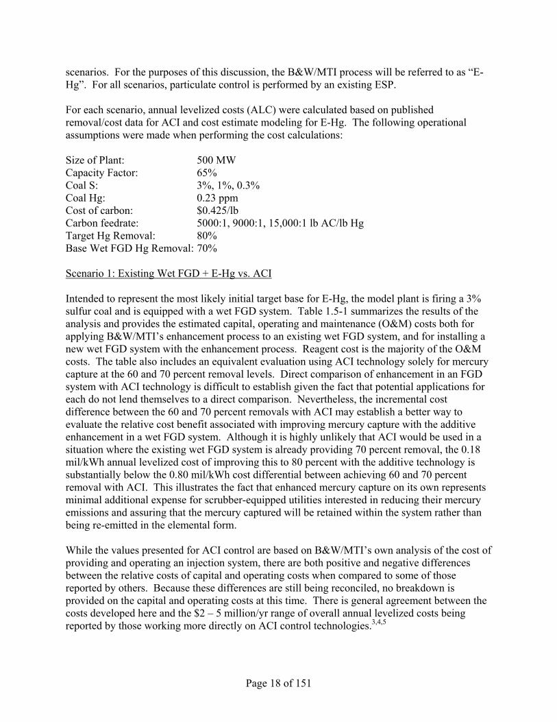
scenarios. For the purposes of this discussion, the B&W/MTI process will be referred to as “E-Hg”. For all scenarios, particulate control is performed by an existing ESP. For each scenario, annual levelized costs (ALC) were calculated based on published removal/cost data for ACI and cost estimate modeling for E-Hg. The following operational assumptions were made when performing the cost calculations: Size of Plant: 500 MW Capacity Factor: 65% Coal S: 3%, 1%, 0.3% Coal Hg: 0.23 ppm Cost of carbon: $0.425/lb Carbon feedrate: 5000:1, 9000:1, 15,000:1 lb AC/lb Hg Target Hg Removal: 80% Base Wet FGD Hg Removal: 70% Scenario 1: Existing Wet FGD + E-Hg vs. ACI Intended to represent the most likely initial target base for E-Hg, the model plant is firing a 3% sulfur coal and is equipped with a wet FGD system. Table 1.5-1 summarizes the results of the analysis and provides the estimated capital, operating and maintenance (O&M) costs both for applying B&W/MTI’s enhancement process to an existing wet FGD system, and for installing a new wet FGD system with the enhancement process. Reagent cost is the majority of the O&M costs. The table also includes an equivalent evaluation using ACI technology solely for mercury capture at the 60 and 70 percent removal levels. Direct comparison of enhancement in an FGD system with ACI technology is difficult to establish given the fact that potential applications for each do not lend themselves to a direct comparison. Nevertheless, the incremental cost difference between the 60 and 70 percent removals with ACI may establish a better way to evaluate the relative cost benefit associated with improving mercury capture with the additive enhancement in a wet FGD system. Although it is highly unlikely that ACI would be used in a situation where the existing wet FGD system is already providing 70 percent removal, the 0.18 mil/kWh annual levelized cost of improving this to 80 percent with the additive technology is substantially below the 0.80 mil/kWh cost differential between achieving 60 and 70 percent removal with ACI. This illustrates the fact that enhanced mercury capture on its own represents minimal additional expense for scrubber-equipped utilities interested in reducing their mercury emissions and assuring that the mercury captured will be retained within the system rather than being re-emitted in the elemental form. While the values presented for ACI control are based on B&W/MTI’s own analysis of the cost of providing and operating an injection system, there are both positive and negative differences between the relative costs of capital and operating costs when compared to some of those reported by others. Because these differences are still being reconciled, no breakdown is provided on the capital and operating costs at this time. There is general agreement between the costs developed here and the $2 – 5 million/yr range of overall annual levelized costs being reported by those working more directly on ACI control technologies.3,4,5

Page 19 of 151

Table 1.5-1: Costs of Mercury Removal Processes ENHANCED MERCURY

CAPTURE IN A WET FGD SYSTEM

Existing 500 MW Installation

New 500 MW Installation

Total Capital Requirement, $ 3,000,000 63,000,000

Total System O&M Costs, $/yr 125,000 3,200,000

Annual Levelized Cost, $/yr 500,000 12,000,000

Annual Levelized Cost, mil/kWh 0.18 4.23

MERCURY CAPTURE WITH ACI TECHNOLOGY @ 60% Removal @ 70% Removal

Annual Levelized Cost, $/yr 2,400,000 4,700,000

Annual Levelized Cost, mil/kWh 0.85 1.65 The application of the B&W/MTI enhanced mercury capture process with a wet FGD system has the additional benefit of having virtually no impact on scrubber operation and gypsum quality. Moreover, it does not adversely affect the acceptability of fly ash for disposal/sale, a potential drawback ACI may have if it is not practical or economically attractive to separate by-product fly ash from the spent activated carbon. This aspect came to light in the demonstration of ACI at Wisconsin Electric’s Pleasant Prairie Power Plant where the carbon prevented its use as a cement admixture. The economic impact in this case was estimated to be $12 to $15 million/yr due to lost fly ash sale revenue and increased landfill disposal costs.4 Scenario 2: New Wet FGD + E-Hg vs. ACI + Spray Dryer Absorber (SDA) As further reductions in U.S. SO2 emissions become more likely to be enacted, the installation of additional FGD capacity becomes more likely. In effect, the ‘threshold’ coal sulfur level, above which some type of FGD system would be required, would continue to decrease. As a result, new FGD systems would, in more and more cases, become financially attractive as the amount of low-sulfur coal would continue to decrease and demand increase. In some instances, especially for units already firing lower sulfur coal, spray dryer absorbers (SDA) tend to be favored over wet FGD systems. If mercury control legislation is enacted in conjunction with more stringent SO2 emissions requirements, however, the choice of equipment becomes more interesting. This scenario represents a potentially significant portion of the current U.S. generating market. For example, focusing solely on unscrubbed, ESP-equipped units east of the Mississippi firing bituminous coals encompasses 109,000 MW, one-third of the current generating capacity in the U.S. In this scenario, a 1% sulfur coal is being fired in the 500 MW model plant. For the ACI + SDA options, it has been assumed that the addition of the SDA system will result in Hg removal performance comparable to wet FGD. In Table 1.5-2, the ALC (expressed in mil/kWh and $/yr) are shown for this comparison.

Page 20 of 151

Table 1.5-2: Comparison of Wet FGD + E-Hg vs. ACI + SDA

ALC Wet FGD @ 70% Wet FGD + E-Hg @ 80%

ACI + SDA @ 70%

ACI + SDA @ 80%

mil/kWh 4.05 4.23 4.11 4.59 $/yr, 000’s 11,559 12,063 11,720 13,090 mil/kWh ∆, 70% to 80% 0.18 -- 0.48 $/yr, 000’s ∆, 70% to 80% 504 -- 1,370

The results shown in Table 1.5-2 illustrate two observations. First, the addition of a wet FGD system (with or without E-Hg) for combined SO2 and Hg control is economically competitive with similarly performing ACI + SDA systems. Factoring in potential operational cost increases such as the ash disposal concerns mentioned in Scenario 1, and the application of a wet FGD-based system becomes even more attractive. Secondly, increasing the Hg removal performance for the wet FGD-based system through the addition of E-Hg is significantly less expensive than increasing the carbon feed rate to achieve the same performance for the ACI + SDA system. Scenario 3: New Wet FGD + E-Hg vs. ACI In some instances with low-sulfur coal and SO2 credit surplus, more stringent SO2 emissions regulations will not require utilities to install new FGD control equipment. Any new equipment would be installed primarily for Hg control. For this scenario a 0.3% sulfur coal is being fired in the 500 MW model plant. A large portion of the low-sulfur coal is from the Western U.S. (sub-bituminous) where a much larger percentage of the mercury present in the flue gas is in the elemental form, which is not readily removed by wet FGD systems. Removal performance for the wet FGD estimates have been lowered to reflect an assumed 50:50 split between oxidized and elemental mercury. This does not affect wet FGD costs, only the corresponding ACI system. Similar to Scenario 2, this type of plant (low-sulfur, sub-bituminous coal, non-scrubbed, ESP-equipped) represents a potentially significant portion of the U.S. generating market (86,000 MW).

Table 1.5-3: Comparison of Wet FGD + E-Hg vs. ACI

ALC Wet FGD @ 50%

Wet FGD + E-Hg @ 60% ACI @ 60%

mil/kWh 4.05 4.23 0.85 $/yr, 000’s 11,559 12,063 2,426

SO2 credit, $/yr 000’s 946 946 --

Given the significant capital requirement for wet FGD systems, it is not surprising that installing these systems solely for Hg control will not generally be economically viable. Only in those situations where an increase in carbon content in the fly ash would result in significant operating cost increases (higher disposal costs, loss of by-product sale, etc.) would it potentially become attractive to install wet FGD for Hg control.

Page 21 of 151

2.0 INTRODUCTION 2.1 BACKGROUND AND OBJECTIVES

A wide range of mercury emissions control performance for wet scrubbers in coal applications (0–96%) appear in the literature with a number of factors contributing to this variability. For example, significant differences in the mercury content of U.S. coals result in a wide range of mercury concentrations in the flue gas from the boiler. In addition, the form or species of mercury (elemental mercury or an oxidized compound such as HgCl2) in the flue gas can affect wet FGD system mercury removal efficiency. Mercury speciation in the flue gas can be influenced by the type of coal fired, with sub-bituminous coal generating a higher relative proportion of elemental mercury than bituminous coal. The coal chlorine content and ash characteristics may also influence partitioning between the solid and vapor phases and the mercury species in the vapor phase. Finally, the scrubber spray tower configuration, liquid-to-gas ratio, and slurry chemistry may also impact the reported mercury emissions. Wet FGD systems are currently installed on about 25% of the coal-fired utility generating capacity in the U.S., representing about 15% of the number of coal-fired units. Depending on the effect of the operating parameters mentioned above, FGD systems can provide cost-effective, near-term mercury emissions control options with a proven history of commercial operation. For boilers already equipped with FGD systems, the incremental cost of any vapor phase mercury removal achieved is minimal. To be widely accepted and implemented, technical approaches that improve mercury removal performance for wet FGD systems should also have low incremental costs and have little or no impact on operation and SO2 removal performance. The ultimate goal of this project was to commercialize methods for the control of mercury in coal-fired electric utility systems equipped with wet flue gas desulfurization (wet FGD). The two specific objectives of the project were 1) ninety percent (90%) overall system mercury removal and 2) costs below ¼ to ½ of today’s competing activated carbon mercury removal technologies. Overall system mercury removal is based on the mercury entering the system with the coal and the mercury leaving the system in the stack gas. In other sections, total mercury removal refers to the combined removal of the oxidized, elemental, and particulate mercury in the gas phase across the wet scrubber system.

2.2 BENEFITS OF THE B&W/MTI ENHANCED WET FGD MERCURY REMOVAL PROCESS

The primary benefit from the B&W/MTI enhanced wet FGD mercury removal process is the reduction of mercury emissions from coal-fired utility power plants. Other benefits are described below: Cost-effective. B&W/MTI’s technology is cost-effective because: • Use of existing equipment. Little additional equipment will be required for implementation.

Page 22 of 151

• Low capital cost. Because the technology requires little additional equipment and only minor modification of existing equipment for installation, capital costs are extremely low.

• Low operating cost. Currently, the most promising technology for mercury control alone is

assumed to be activated carbon injection. Unfortunately, sorbent costs are high for carbon injection. The reagent used in B&W/MTI’s technology is low in cost and readily available for application of the technology.

Co-Pollutant Control. Multiple pollutant analysis was recently documented in a report prepared by the U. S. EPA entitled, “Analysis of Emissions Reduction Options for the Electric Power Industry.” The study looked at options to lower air emissions of sulfur dioxide (SO2), fine particulate, mercury, and carbon dioxide (CO2). The basic conclusion to the analysis was that an integrated, multi-pollutant approach to the control of these emissions could offer significant cost savings relative to a piecemeal approach. That conclusion applies directly to the use of wet FGD systems rather than activated carbon for mercury control since wet scrubbers capture multiple pollutants while activated carbon systems are normally applied for species at low concentrations, such as mercury. Compatible with Current Emissions Control Technologies. The approach is ideally suited to wet FGD systems, since it utilizes existing equipment and provides mercury control with a proven history of commercial operation. The technology can be easily applied to both existing and new wet FGD systems from any supplier. All testing to date indicates that this approach has no adverse effects on wet scrubber performance or operation. Performance Not Adversely Affected by Change in Power Plant Systems. In general, the power plant systems do not affect the mercury removal performance of the B&W/MTI enhanced wet FGD mercury removal technology. Furnace configuration, burner type, and plant size should have no effect on performance. No Adverse Impact to By-Product Disposal or Usage. The B&W/MTI enhanced wet FGD mercury removal technology would not adversely affect the acceptability of the fly ash or gypsum products for sale while competing technologies such as activated carbon injection have the potential to dramatically increase the cost of disposal and/or limit its resale value. 2.3 PROJECT SPONSORS The Full-scale Testing of Enhanced Mercury Control for Wet FGD Systems Program was funded by the U.S. Department of Energy’s National Energy Technology Laboratory, the Ohio Coal Development Office within the Ohio Department of Development, and Babcock & Wilcox. Host sites and associated support were provided by Michigan South Central Power Agency and Cinergy.

Page 23 of 151

3.0 TECHNICAL DISCUSSION 3.1 PROCESS DESCRIPTION B&W/MTI’s enhanced wet FGD mercury removal process adds very small amounts of a proprietary reagent to an existing wet FGD system to increase mercury removal efficiency. 3.2 TECHNICAL APPROACH

3.2.1 Overview The goal of this project was to conduct full-scale, long-term, field-testing of B&W/MTI’s enhanced wet FGD mercury removal technology to obtain mercury removal performance and cost data. Field-testing was completed at two commercial coal-fired utilities with wet FGD systems: 1) MSCPA’s 55 MWe Endicott Station and 2) Cinergy’s 1300 MWe Zimmer Station. Testing was conducted at these two locations because of the large differences in size and wet scrubber chemistry. Endicott employs a limestone, forced oxidation (LSFO) wet FGD system, whereas Zimmer uses Thiosorbic Lime (magnesium enhanced lime) and ex situ oxidation. Both locations burn Ohio bituminous coal. Table 3.2-1 compares the characteristics of the two test locations.

Table 3.2-1: Test Location Characteristics Comparison

MSCPA Endicott Station

Cinergy Zimmer Station

Electricity Generation 55 MWe 1300 MWe

Number of Wet Scrubber Modules 1 6

Wet Scrubber Reagent Limestone Thiosorbic Lime

Wet Scrubber Oxidation Method In situ Forced Oxidation

Ex situ Forced Oxidation

Wet Scrubber Liquid-to-gas Ratio 78 gal/1000 acf 21 gal/1000 acf

Slurry pH 5.4 – 5.6 5.8 – 6.0

Inlet SO2 Concentration 3600 ppm 3300 ppm

Gypsum Use Cement Wallboard MSCPA Endicott Station. Figure 3.2-1 shows MSCPA’s Endicott Station. The plant is located in Litchfield, Michigan, approximately 40 miles southwest of Jackson, Michigan. Commercial operation began in November 1982. The power plant is rated at 60 MWe and typically produces 50-55MWe during the day and 30 MWe at night. Approximately 140,000 tons of Ohio

Page 24 of 151

bituminous coal are burned per year. The coal’s higher heating value is 12,000 Btu/lb (as received) with a sulfur content of about 3%. The power plant is equipped with one B&W Stirling boiler, producing 480,000 lb/hr steam at 950°F and 1450 psig. A single ABB turbine handles the steam-to-electric power conversion. The Endicott plant’s air pollution control equipment includes one dry electrostatic precipitator and one wet scrubber. The precipitator is a Belco cold-side unit, having a flyash removal efficiency greater than 98%. It has three transformer-rectifiers rated at 38.5 KVA and five transformer-rectifiers rated at 58.5 KVA. No gas conditioning is used for precipitator operation. A single absorber, in situ forced oxidation B&W wet scrubber is used for sulfur dioxide control. The reagent used is limestone slurry that is prepared in a crusher, tower mill, and classifier system. SO2 removal is regulated at ninety (90%) percent with the wet FGD system typically achieving 92% SO2 removal without the use of any additives. Primary dewatering is achieved with a thickener and secondary dewatering is accomplished with two Dorr-Oliver rotary drum vacuum filters. Approximately 28,000 tons/year of gypsum are produced and sold to concrete and agricultural concerns.

Figure 3.2-1: MSCPA Endicott Station, Litchfield, Michigan Cinergy Zimmer Station. Figure 3.2-2 shows Cinergy’s Zimmer Station. The Cinergy Zimmer Station is located in Moscow, Ohio, 30 miles southeast of Cincinnati. The Zimmer generating station, rated at 1300 MWe, was the world’s first nuclear-to-coal conversion. The plant began

Page 25 of 151

commercial operation in March 1991 and burns 3.5 million tons of Ohio bituminous coal per year. The power plant is equipped with a single B&W Carolina-type Universal Pressure boiler that produces 9775 million pounds of steam per hour at 1000°F and 3690 psig. The turbine generator system incorporates a Westinghouse low-pressure turbine generator set from the nuclear cycle with a new ABB high and intermediate pressure turbine generator. The Zimmer station’s air pollution control equipment includes two electrostatic precipitators for particulate control and six B&W wet scrubbers modules for SO2 control, installed at the same time as the boiler and turbine. The precipitators are Flakt cold-side units having a 99.9% flyash removal efficiency. No gas conditioning is used for precipitator operation. The scrubbers employ Thiosorbic (magnesium-enhanced) lime slurry as the reagent. The reagent preparation system consists of ball mills, classifiers, and slurry storage tanks. SO2 removal efficiency is typically controlled at 92%, but the unit is capable of 95% removal efficiency with five absorbers operating. The Zimmer wet FGD system was initially equipped and operated with thickeners for primary dewatering, and drum-type vacuum filters for secondary dewatering. In 2000, the dewatering system was upgraded by B&W to include an ex situ forced oxidation system to produce gypsum using hydroclones for primary dewatering and belt filters for secondary dewatering. The ex situ forced oxidation system was operational for this project.

Figure 3.2-2: Cinergy’s Zimmer Station, Moscow, Ohio

Page 26 of 151

3.2.2 Field Operation Phases Figure 3.2-3 shows the project schedule and illustrates the testing phases necessary to demonstrate the commercial success of the B&W/MTI enhanced wet FGD mercury removal process. Field operation began at the Endicott Station. The phases of operation at the Endicott Station were as follows:

• Parametric testing to define the optimal operating parameters for the process.

• Two weeks of verification testing to verify the performance of the process with the selected operating conditions.

• Four months of long-term operation to continue the verification of the amount of mercury

removal achieved and to prove that there were no long-term effects on SO2 removal, materials of construction, or by-product utilization.

After completing field operation at the Endicott Station, the B&W/MTI enhanced mercury removal system was moved to the Zimmer Station for testing. Field operation at the Zimmer Station included:

• Two weeks of verification testing to verify the performance of the process with the selected operating conditions. Reagent was added to all operating wet scrubbers modules simultaneously.

Task NameDesign and Fabrication

Design

Fabrication

Field OperationEndicott Station

Parametric

Verif ication

Long-Term

Zimmer StationVerif ication

Data AnalysisOntario Hydro Chemistry

Data Reduction

Process Stream Chemistry

Reporting

S O N D J F M A M J J A S O N D J F M A M J2001 20

Figure 3.2-3: Project Schedule

Page 27 of 151

3.2.3 Mobile Test Pump Skid To facilitate minimal construction and set-up at each plant site, a mobile equipment skid was fabricated to connect to the existing wet scrubber systems at the Endicott and Zimmer Stations. A picture of the equipment skid is shown in Figure 3.2-4. An equipment drawing is shown in Figure 3.2-5.

Figure 3.2-4: Reagent Injection Skid A tank truck of additive solution was used as the on-site storage vessel. A NPS chemical transfer hose was used to connect the skid to the additive tank truck, plant water system, and wet FGD absorber recirculation piping. Stainless steel piping was used to connect the components on the skid. A large and small additive injection/metering pump were mounted on the skid, one for the MSCPA Endicott test, and one for the Cinergy Zimmer test. The pumps were equipped with variable frequency controllers, which permitted a 100:1 turndown. The skid was also equipped with a dilution water system for added flexibility in varying additive feed concentration. A calibration tube was provided upstream of the pumps to check pump delivery rates. A pulsation dampener, having a flexible elastomeric bladder/diaphragm and a gas-pressurized upper chamber, was located in the pumps’ common discharge line to facilitate a more uniform feed flow. Also provided were flow meters, flow control valves, pressure regulating valves, pressure

Page 28 of 151

gauges, and a pressure relief valve. All equipment, pipe, valves and fittings were made of 316 stainless steel, with suitable elastomers where required. Only minor modifications to the existing wet FGD equipment were required to connect the reagent feed line to the plant’s slurry system. After testing was complete, the hose connections to the tank truck, absorber recirculation pump suctions and plant water supply were disconnected, the skid’s power hook-up was detached, and the skid was shipped to MTI for storage. It is available for future testing.

Page 29 of 151

Figure 3.2-5: Reagent Injection Skid Equipment Schematic

Page 30 of 151

3.2.4 Ontario Hydro Measurements – General Methodology The Ontario Hydro (OH) Method was used to measure total and speciated mercury emissions during all testing phases of this program. A variation of EPA Method 29, this method applies to the determination of particulate and gaseous metals emissions from industrial, utility, and municipal sources. Particulate and gaseous emissions are withdrawn isokinetically from a source and pass through a quartz fiber filter and solutions of potassium chloride (KCl), acidic peroxide and acidic potassium permanganate (KMnO4). The oxidized forms of mercury collect in the KCl impingers and elemental mercury collects in the peroxide and potassium permanganate impingers. Highlights of the procedures used in the method include:

• Potassium permanganate was added to the KCl impingers immediately after the post-sampling leak check to prevent the loss of oxidized mercury during recovery of the sample. Typically, 3-6 ml of KMnO4 were needed to achieve the desired purple endpoint.

• A nominal sampling time of two hours was used at all locations. The mercury collected

in the impingers remained well above the analytical detection limits.

• The particulate filter was maintained at the flue gas temperature (to a maximum of 340 °F) or a minimum of 275 °F.

• Nozzle diameters were selected to achieve a target isokinetic sampling rate of 0.5 to 0.6

dscfm (dry standard cubic feet per minute).

• The same sampling probe assembly was used at a given location for each test to minimize variation between runs that may result from the breakdown and reassembly of different sampling equipment.

The impinger solutions from the Ontario Hydro Method sample trains were analyzed for mercury using Cold Vapor Atomic Absorption Spectroscopy (CVAAS). This method was used to determine both the elemental and ionic forms of mercury. The analysis follows EPA reference method SW7470 (CVAAS). The flue gas sampling port locations and planned traverse points were consistent (to the extent that the duct sizes can be traversed with normally available equipment) with EPA Method 1 - Sample and Velocity Traverses for Stationary Sources. Method 1 specifies the minimum number of traverse points required for the flue diameter and proximity to flow disturbances. The sampling details for each location at each of the demonstration sites are summarized in Table 3.2-2. Sampling performed at both stack locations was conducted through 4 sample ports, located 90° from each other around the circumference of the stack. Sampling performed at both inlet locations was conducted through multiple ports in the same plane (as indicated in the table).

Page 31 of 151

Table 3.2-2: Flue Gas Sampling Details

MSCPA – Endicott Station Cinergy – Zimmer Station

Wet FGD

Inlet

Wet FGD

Outlet (Stack)

Wet FGD

Inlet

Wet FGD

Outlet (Stack)

Flue Dimensions (W x D), ft. 8 x 10.75 -- 37.5 x 37.5 -- Stack Diameter, ft. -- 10 -- 42.7 Flue Orientation Vertical -- Horizontal -- Port Diameter (in.) 4 4 4 4 Number of Ports 5 4 3 4 (2 used) # Traverse Points 25 (5 x 5) 12 (4 x 3) 12 (3 x 4) 12 (2 x 6) # Sampling Planes 1 1 1 1 Gas Temperature (°F) 350 - 370 120 - 130 330 - 350 120 – 130 Nominal Pressure (in. H2O) -7 +0.4 -19 -0.9 Filter Temperature (°F) 340 275 340 275

Sample train and equipment preparation and recovery took place in a fully equipped, mobile laboratory trailer shown in Figures 3.2-6 and 3.2-7.

Figure 3.2-6: Laboratory Trailer (Exterior)

Page 32 of 151

Figure 3.2-7: Laboratory Trailer (Interior)

3.2.5 PS Analytical Mercury Analyzer System An on-line mercury analyzer system, manufactured by PS Analytical (PSA), was used during field-testing with the hope of obtaining real-time mercury trending. PSA first introduced the amalgamation atomic fluorescence spectrometer for gaseous phase measurement of total mercury in 1991. It was initially used for ambient air and natural gas sampling. The basic principle of operation is that gas samples are drawn across a gold trap (Amasil tube) to capture mercury. The trap is then heated to release mercury that is delivered to an atomic fluorescence detector. In 1996, PSA introduced a system for on-line measurement of mercury in flue gas from coal-fired boilers. Final design of the system continues with input from the Energy and Environmental Research Center (EERC) at the university of North Dakota, B&W/MTI, and U.S. DOE. The specifications for the instrument are in Table 3.2-3. A schematic arrangement of the current design for on-line speciation/total mercury determination is shown in Figure 3.2-8 and a photograph of the analyzer is shown in Figure 3.2-9.

Page 33 of 151

Table 3.2-3: PS Analytical Mercury Analyzer Specifications

Detection Limit: 5ng/m3 (2.5 liter sample)

Linear Range: 300 µg/m3 (2.5 liter sample)

Sampling Frequency: 5 minutes

Gas Requirements: 0.8 l/min-1 Argon, Nitrogen or Air

Calibration Techniques: Vapor Injection – Absolute

Permeation source with concentration range selection

Reductant (for total Hg): 2 ml/min (Speciation Accessory)

Buffer (for Hg0): 2 ml/min (Speciation Accessory)

Relative Accuracy: Within ±15% of EPA Methods

Figure 3.2-8: PS Analytical Mercury Analyzer Schematic

Stack

Heated SampleProbe

Conversion and Drying Unit

Reagent Transfer

Assembly

Industrial P C

Sir Galahad II

C001K001CavKit

Calibration Assembly

MFC*VacuumPump

* Mass Flow Controller

Page 34 of 151

Figure 3.2-9: PS Analytical Mercury Analyzer The PSA Mercury Analyzer System did not perform as expected throughout this program. The analyzer itself performed very well, but there were a host of problems with the preconditioning system. At no time during the six-month project did the system perform well enough to have confidence in using the data to make a definitive statement about the mercury removal process or plant performance. Therefore, this section will be dedicated to “lessons learned” in the hope that some of the improvements made to the system will benefit others. It is assumed that the reader is familiar with the PSA equipment and gas sampling methods in the following discussion. 1. SO3 Aerosol – Both Zimmer and Endicott have reported high levels of SO3 in the flue gas.

When this gas is cooled, as occurs in the preconditioner impingers, the SO3 condenses and forms an aerosol that is not scrubbed by the impingers. This aerosol eventually built up on the walls of the long (175 ft) transfer lines, absorbed water vapor to form sulfuric acid, and scrubbed mercury out of the gas sample. The build up of acid was verified by flushing the lines with distilled water and measuring the pH of the flush water which was often as low as 2. To alleviate this problem, the connection between the precondition oven and impingers was modified to include a coil of ⅛-inch tubing. The purpose of the coil was to

Page 35 of 151

act as an inertial separator to remove the aerosol by forcing it to collide with the tubing walls.

2. Peltier Upgrade – Early in the test, condensation in the transfer lines caused several

problems. The Peltier coolers were upgraded to double the cooling capacity. It is important that the treated gas be completely dry if long transfer lines are used.

3. 3-Way Solenoid Valve – Several times during the project the drains on the Peltier coolers

plugged with various kinds of precipitate, and overflowed. Normally, this did not cause a serious problem because the overflow trips a moisture sensor and shuts down the chemical pumps. However, this particular system is configured so that the gas pump remains on. If not corrected, moisture in the flue gas continues to condense in the cooler and overflows into the transfer line along with the impinger chemicals. Eventually, the overflow floods the switch box and the analyzer gold trap, necessitating cleaning and repair. To correct this problem Teflon®, 3-way solenoid valves were incorporated into the system so that a trip of the moisture sensors also switched the 3-way valve to divert the gas flow into a waste container.

4. Black Precipitate – Early in the test, the cooler drain plugged several times with a black

precipitate. The impinger chemistry was adjusted to avoid precipitation. 5. White/Yellow Precipitate – On several occasions, a whitish/yellow deposit formed on the

impinger glassware. The material was very difficult to dissolve in either acids or bases. At the time, it was believed that the deposit had no effect on Hg because the impinger chemistry is designed to evolve all mercury. However, in a later discussion with other mercury CEM users, it was learned that this deposit could absorb mercury and, in fact, could explain some of the strange behavior seen on several occasions. For example, on one occasion an ID fan at Zimmer tripped and caused an emergency shut down of the entire plant. Immediately after the trip, the mercury value spiked off-scale and remained there for several hours even though the analyzer was only sampling air. One explanation is that in normal operation the impinger chemistry reduced some of the SO2 in the gas to sulfur that deposited on the glassware and tubing. The sulfur absorbed some of the mercury and gradually built up. The reaction stayed in relative equilibrium as long as the chemistry remained constant. However, when the boiler tripped, the source of sulfur was eliminated and the deposit began to dissolve releasing the trapped mercury back into the gas. This not only explains this one strange occurrence, but can also account for the low mercury values, as compared to the O-H measurements, seen throughout the project. The best comparisons ever obtained during the project were only about half of the Ontario Hydro Method values. Since this problem was not identified until after the project, it is uncertain how to correct for it.

6. Cool Spots – Early in the test, the measured mercury would occasionally spike to high

values for short periods. These spikes were identified by the manufacturer as an indication of a cool spot before the impingers. It is postulated that oxidized mercury condenses in cool spots and builds up until it is swept into the impinger with water droplets. Several modifications were tested, but the one that worked best involved better insulation between

Page 36 of 151

the oven and impinger, increasing the velocity between the oven and impinger by replacing a short length of ¼-inch tubing with ⅛-inch tubing, and installing an ⅛-inch T immediately after the oven. Water was injected into the bottom of the T to quickly quench the gas.

7. Long Transfer Lines – 175 ft, heated, Teflon® sample hoses were used to transport the

conditioned gas from the preconditioners to the analyzer in the lab trailer. Tests with gas spiked with Hg0 from the PSA CAV Kit showed that the transfer lines did absorb some mercury, especially if they were contaminated with acid from the flue gas. The only solution to this is to locate the analyzer and preconditioners as close to the sample points as possible, but this is often very costly or logistically unfeasible.

8. Ash Filter – On several occasions the mercury values would suddenly drop. Often times,

but not always, this could be corrected by replacing the particulate filter in the heated sample box. These occurrences could not be consistently correlated to anything happening in the plant, like soot blowing, bringing on or taking off a burner, switching pulverizers, etc., but it is likely related to some combustion situation that produces soot or unburned carbon that collects on the filter and absorbs mercury. The color of ash deposits on the filter varied from almost white to black. To minimize this, the filter was changed before every set of O-H tests. Apogee makes a “virtual” filter that may have merit in this application.

3.3 ONTARIO HYDRO FLUE GAS SAMPLING RESULTS In the following sections mercury speciation and removal data are shown in several figures. Unless otherwise indicated, the following figure description will apply: • Each pair of bars in a given figure represents the average wet FGD inlet and outlet

total gas phase mercury concentrations for a given test. Each bar is further divided to show oxidized and elemental mercury concentrations. The number above the outlet bar represents the average total mercury removal across the wet FGD system for that test. The error bars represent the maximum and minimum total mercury concentration for each location and each test.

• During the course of the program, particulate phase Hg concentrations were also

determined at the wet FGD systems inlet and outlet. These concentrations averaged less than 1% of the total present in the flue gas and thus are not shown in the figures in the following sections.

3.3.1 MSCPA, Endicott Station 3.3.1.1 MSCPA Test Plan Three phases of testing were conducted at the Endicott Station: Parametric, Verification, and Long-Term. The purpose and objectives of these phases were as follows:

Page 37 of 151

• Parametric – testing completed over a range of reagent feed rates to achieve three

incremental mercury removal levels between 40% and 90% and to provide performance curve and cost data. In all, 8 tests were completed during this phase. A summary of the parametric tests and number of O-H sample trains conducted during each test is given in Table 3.3-1.

Table 3.3-1: Summary of Parametric Tests – Endicott

Test ID Reagent Feed Rate, gph No. of Inlet Trains No. of Outlet Trains

5/8/01-1 Baseline, (0.0 gph) 3 4 5/16/01-2 2.9 2 2 5/17/01-3 0.29 3 3 5/18/01-4 0.07 3 3 6/11/01-5 Baseline, (0.0 gph) 3 3 6/12/01-6 0.18 2 2 6/13/01-7 0.29 3 3 6/14/01-8 1.0 2 3

• Verification – testing began immediately following the Parametric test phase to demonstrate

consistent day-to-day operation and mercury removal performance. This phase spanned 16 days; 14 sets of inlet and outlet OH sample trains (one set per day) were conducted.

• Long-Term – following the completion of the Verification test phase, four months of long-

term operation were conducted to not only continue verification of mercury removal performance, but to demonstrate that there were no long-term deleterious effects on SO2 removal, materials of construction, or by-product utilization. During this test phase, 8 tests were conducted with triplicate sets of OH sample trains performed for each test.

For all phases of the test program conducted at Endicott, OH sampling was conducted at both the wet FGD inlet (upstream of the ID fan) and wet FGD outlet (on the stack). Pictures of each sampling location are shown in Figures 3.3-1 (inlet) and 3.3-2 (outlet). In Figure 3.3-1 the 5 inlet sampling ports are located behind the narrow horizontal strip of lagging material.

Page 38 of 151

Figure 3.3-2: Wet FGD Outlet (Stack) Sampling Location - Endicott

Figure 3.3-1: Wet FGD Inlet Sampling Location - Endicott

Page 39 of 151

3.3.1.2 Plant Operation A summary of the major operating parameters for the 3 test phases conducted at Endicott is shown in Table 3.3-2 (all of the Endicott DAS data may be found in Appendix B). Each line in the table corresponds to a set of inlet and outlet O-H sample trains. The listed value for a given operating parameter from a specific test represents the average of values stored by the data acquisition system (at 15 second intervals) during that test. For the Parametric and Long-Term tests, triplicate sets of O-H measurements were conducted (except as indicated); these are indicated by the letter ‘A’, ‘B’, or ‘C’ within the Test ID value. For example, the Test ID ‘051701-3B’ refers to the second set of O-H inlet and outlet sample trains, conducted during Test 3 on May 17, 2001. Whenever possible, tests were conducted with the plant at full-load. Tests conducted at less than full-load conditions, especially during the Verification tests, were due to reduced grid power requirements.

Page 40 of 151

Table 3.3-2: Summary of Plant Operating Conditions – Endicott

Ontario Hydro Reagent Flow Plant CO2 In Plant CO2 Out Plant SO2 In Plant SO2 OutPlant SO2

Removal Efficiency

Plant Load WFGD Temp In

Plant Temp Stack

Test ID gph % % ppm (wet) ppm (wet) % MW oF oF

Parametric Tests050801-1A 0.00 10.3 12.3 1206 88 93.9 59 358 116050801-1A1 0.00 10.0 12.0 1218 120 91.8 56 359 117050901-1B 0.00 9.7 12.1 1387 130 92.5 59 354 116050901-1C 0.00 9.5 11.9 1520 144 92.4 61 361 118050901-1D 0.00 9.4 11.9 1438 137 92.5 60 368 119051601-2A 2.93 9.3 11.7 1543 172 91.1 59 358 118051601-2B 2.90 8.9 11.4 1605 187 90.9 55 350 118051701-3A 0.29 9.3 11.8 1797 196 91.4 58 352 119051701-3B 0.30 9.7 12.0 1700 177 91.5 58 361 121051701-3C 0.30 10.0 12.1 1616 164 91.6 59 371 123051801-4A 0.07 9.5 11.8 1647 179 91.3 57 352 120051801-4B 0.06 9.5 11.8 1668 189 90.9 58 357 119051801-4C 0.06 9.8 11.8 1710 184 91.1 56 357 120061101-5A 0.00 9.3 11.9 2385 396 87.3 56 351 121061101-5B 0.00 9.3 11.8 2047 200 92.3 53 358 123061101-5C 0.00 9.3 11.9 1815 234 89.9 56 367 123061201-6A 0.17 9.8 11.9 1793 172 92.1 56 352 120061201-6B 0.17 10.0 12.0 1681 155 92.3 55 362 122061301-7A 0.29 9.9 12.1 1449 157 91.2 54 355 122061301-7B 0.26 9.7 11.9 1626 197 90.2 53 361 123061301-7C 0.30 9.6 11.9 1553 149 92.3 53 371 124061401-8A 1.01 9.8 12.0 1568 155 91.9 53 352 122061401-8B 1.04 10.0 12.0 1448 144 91.8 53 362 122061401-8C 1.02 10.0 12.1 1605 164 91.5 53 364 122Verification Tests062501-9A 1.03 10.1 13.0 1983 204 92.0 57 375 122062601-10A 1.01 9.8 12.7 2052 259 90.3 56 364 121062701-11A 0.99 12.6 11.3 1917 134 94.9 55 365 122062801-12A 1.00 11.9 10.9 1827 191 87.5 57 360 121062901-13A 1.00 11.8 10.4 1916 146 91.3 55 361 122063001-14A 1.00 11.7 10.1 1683 124 91.4 55 366 124070101-15A 1.00 10.4 8.9 1634 95 93.3 38 332 117070201-16A 1.00 11.3 10.4 1904 117 93.3 44 322 112070601-17A 1.00 12.4 9.8 1711 100 92.6 47 340 118070701-18A 1.00 11.3 8.9 1489 76 93.5 37 322 117070801-19A 1.00 11.6 9.4 1552 84 93.3 44 359 122070901-20A 1.00 12.1 11.8 1945 138 92.7 57 364 122071001-21A 1.00 11.8 10.5 1690 102 93.2 56 365 122071101-22A 1.00 10.4 10.8 1820 126 93.3 58 355 118Long Term Tests071201-23A 1.00 12.2 11.2 1935 140 92.1 57 349 118071201-23B 1.00 12.4 11.4 1980 147 91.9 57 356 119071201-23C 1.00 12.2 11.8 1839 139 92.2 56 362 120072401-24A 1.00 12.4 9.5 2033 125 92.0 57 366 124072401-24B 1.00 12.7 9.4 2175 150 90.7 56 371 125072401-24C 1.00 12.4 9.1 2272 240 85.6 55 376 126080701-25A 1.00 12.0 10.8 1745 130 91.6 48 347 122080701-25B 1.00 12.1 10.4 2095 170 90.6 46 354 124080701-25C 1.00 12.0 10.2 2311 225 88.6 45 360 125082101-26A 0.99 12.3 10.6 1801 130 91.6 54 343 119082101-26B 0.99 12.3 10.5 1984 154 90.9 56 354 120082101-26C 0.99 12.5 10.7 1857 143 91.0 58 366 120090501-27A 1.00 12.4 10.8 1924 149 91.1 56 346 119090501-27B 1.00 12.2 10.8 1911 146 91.3 56 355 120090501-27C 1.00 12.3 10.5 1845 140 91.1 57 365 120091801-28A 1.00 12.2 10.6 1949 153 90.9 57 358 119091801-28B 1.00 12.2 10.6 1982 159 90.8 57 367 119091801-28C 1.00 12.5 10.7 2046 163 90.7 57 373 120100201-29A 1.00 12.8 11.9 2157 233 88.4 59 366 121100201-29B 1.00 12.7 10.9 2091 238 86.8 59 373 121100201-29C 1.00 12.8 10.9 1975 190 88.7 59 377 122100301-30A 0.00 12.5 10.9 2271 214 89.2 56 348 119100301-30B 0.00 12.5 11.0 2374 385 81.6 59 368 121100301-30C 0.00 12.7 11.1 2336 502 75.6 59 374 120

Page 41 of 151

3.3.1.3 Parametric Test Results In Figures 3.3-3 and 3.3-4 the mercury removal performance across the scrubber and speciation results for the 8 parametric tests are shown as a function of reagent feed rate. The first 4 tests (baseline + 3 feed rates) are shown in Figure 3.3-3; the last 4 tests (baseline + 3 feed rates) are shown in Figure 3.3-4. No reagent was injected during the baseline tests. All 8 parametric tests were conducted with the plant operating at full-load (55 MW). Due to problems with the mercury analyzer system, the last four parametric tests were conducted 3 weeks after the first four tests to allow time to analyze the sample trains and interpret the findings. As a result of this delay, a second baseline test was performed to establish a new benchmark for the subsequent tests.

0

3

6

9

12

15

18

21

24

27

30

Base line 0.07 gph 0.29 gph 2.9 gph

Reagent Feed Rate

Gas

Pha

se H

g, µ

g/ds

cm

Oxidized Elemental

62.2% 80.1%83.9%84.0%

Figure 3.3-3: Hg Speciation Summary, Parametric Tests 1 - 4

Page 42 of 151

Several interesting observations are apparent based on the data presented in the above figures. First, the mercury concentration in the flue gas entering the wet FGD system varies widely. For example, even though the 4 tests shown in Figure 3.3-4 were conducted on consecutive days, the average inlet gas phase mercury concentration ranged from 13 to 26 µg/dscm. Because Endicott fires up to four different Ohio coals (at varying sulfur concentrations), primarily based on spot market availability, this level of variation is not entirely unexpected. As a result, judging the effectiveness of the mercury control technology cannot be entirely based on removal performance alone. Consequently, simply comparing the mercury removal performance between the 0.18 gph and 0.29 gph tests shown in Figure 3.3-4 (without further analysis) would yield an erroneous conclusion regarding the reagent performance, namely, decreasing removal performance vs. increasing reagent feed rate. This is due to the fact that oxidized mercury is much more readily captured in wet FGD systems and that there was nearly twice as much oxidized mercury present in the inlet flue gas for the 0.18 gph test than for the 0.29 gph test, resulting in a falsely low bias for the 0.29 gph test. As mentioned previously, the mercury control technology utilized during this program enhances mercury control in two ways: 1) increasing oxidized mercury removal performance, and 2) suppressing the reemission of mercury, already captured by the wet FGD system, in the elemental form. By evaluating the mercury removal performance with respect to the wet FGD outlet flue gas mercury concentration and speciation, a more meaningful performance curve can be generated. In Figure 3.3-5, the average outlet mercury speciation results for the 8 parametric tests are shown as a function of reagent feed rate. In the figure, the two baseline tests have been averaged (the elemental/oxidized ratio for both baseline tests was similar). The upper set of error

0

3

6

9

12

15

18

21

24

27

30

Base line 0.18 gph 0.29 gph 1.0 gph

Reagent Feed Rate

Gas

Pha

se H

g, µ

g/ds

cmOxidized Elemental

79.9% 79.7%73.1%78.8%

Figure 3.3-4 Hg Speciation Summary, Parametric Tests 5 - 8

Page 43 of 151

bars represents the maximum and minimum elemental mercury concentration for each test; the lower represents the maximum and minimum oxidized mercury concentration. The general trend is for decreasing mercury concentration (total, oxidized and elemental) with increasing reagent feed rate. This trend is illustrated more clearly in Figure 3.3-6, utilizing an X-Y plot to show total outlet gas phase mercury concentration as a function of reagent feed rate. The error bars shown in the figure represent the maximum and minimum total gas phase mercury concentration for each test.

Figure 3.3-5: Summary of Wet FGD Outlet Hg Speciation, Parametric Tests

0

1

2

3

4

5

6

7

Base (Avg) 0.07 0.18 0.29 0.29 1 2.9


Gas

Pha

se H

g, µ

g/ds

cm

Oxidized Elemental

Page 44 of 151

In order to conduct the Verification and Long-Term phases of the Endicott demonstration program, it was necessary to determine a reagent feed rate that would 1) provide high mercury removal performance, 2) maintain high removal performance regardless of inlet mercury concentrations, and 3) be low enough to allow a direct scale-up (same reagent/flue gas ratio) for the Zimmer demonstration program using the existing reagent feed system. Thus, although maximum mercury control was achieved with a reagent feed rate of 2.9 gph, the corresponding feed rate for the Zimmer demonstration would have exceeded the design capacity of the feed system. A reagent feed rate of 1 gph was therefore chosen for the Verification and Long-Term phases. With this feed rate the corresponding Zimmer demonstration feed rate fell below the feed system design capacity. Additionally, any fluctuations in inlet mercury concentration would be less likely to adversely affect removal performance, since similar mercury control performance was observed for the 0.29 and 1 gph tests (offering 3 to 4 times the amount of reagent to absorb the impact of concentration fluctuations). 3.3.1.4 Performance Verification Test Results Verification testing, designed to demonstrate consistent day-to-day operation and removal performance, spanned 16 days; 14 sets of inlet and outlet OH sample trains (one set per day, test numbers 9 through 22) were conducted during this period. In Figure 3.3-7 a graphical summary of the speciation results for the 14 verification tests is shown. Each set of bars represents one

Figure 3.3-6: Effect of Reagent Feed Rate on Outlet Hg Concentration - Endicott

0

1

2

3

4

5

6

7

0 0.5 1 1.5 2 2.5 3 3.5


Tot

al O

utle

t Gas

Pha

se H

g, µ

g/ds

cm

Page 45 of 151

inlet and outlet set of OH sample train measurements. The average mercury removal across the wet FGD system for the Verification testing phase was 76%. A tabular summary of the results is given in Table 3.3-3.

0.0

5.0

10.0

15.0

20.0

25.0

30.0

9 10 11 12 13 14 15 16 17 18 19 20 21 22

Test ID

Gas

Pha

se H

g, µ

g/ds

cm

Oxidized ElementalAvg. Removal = 76%

Figure 3.3-7: Summary of Hg Speciation Results - Endicott Verification Tests

Page 46 of 151

Table 3.3-3: Summary of Hg Speciation Results - Endicott Verification Tests

Average Maximum Minimum

Wet FGD Inlet Hg Concentration, µg/dscm

Total 21.7 27.1 17.3 Oxidized 16.2 20.9 11.2 Elemental 5.4 7.4 3.9

Hg Speciation, % Oxidized 75 -- -- Elemental 25 -- --

Wet FGD Outlet Hg Concentration, µg/dscm



Wet FGD Hg Removal, %

Total 76.1 82.3 69.3 Oxidized 93.5 -- -- Elemental 19.5 -- --

The data summaries shown in Figure 3.3-7 and Table 3.3-3 illustrate two important points: 1) the control technology performed as expected with high oxidized mercury removal and suppressed reemission of mercury from the scrubber in the elemental form, and 2) due to the speciation percentages, very high total mercury removal performance across the wet FGD system (>90%) is not possible without some type of mercury oxidation technology upstream of the wet FGD system. These observations will be discussed in greater detail below. In Figure 3.3-8 the effectiveness of the control reagent, at the chosen feed rate of 1 gph, is shown. During the course of the Verification tests, the inlet oxidized mercury concentration ranged from approximately 11 to 21 µg/dscm. Because wet FGD systems capture oxidized mercury much more readily than elemental, large fluctuations in the oxidized mercury concentration will be more likely to affect the overall mercury removal performance. The outlet oxidized mercury concentration remained essentially constant over the range of inlet oxidized

Page 47 of 151

mercury concentrations. This would indicate that the 1 gph feed rate was sufficient to adequately account for the variations in inlet mercury concentration experienced during day-to-day operation by maintaining high levels of oxidized mercury removal across the scrubber, regardless of inlet oxidized mercury concentration.

In Figure 3.3-9, the outlet elemental mercury concentrations from the Verification tests are shown as a function of inlet elemental mercury concentration. A 45° line, representing equal inlet and outlet concentrations, is included in the figure for reference. Data points above and to the left of the 45° reference would represent conditions where mercury is being reemitted from the scrubber in the elemental form; points to the right and below the line correspond to conditions where mercury reemission is suppressed. All but one of the data points fall on or below the 45° line, indicating that mercury reemission was suppressed.

0.0

1.0

2.0

3.0

4.0

5.0

6.0

7.0

8.0

9.0

10.0

10.0 12.0 14.0 16.0 18.0 20.0 22.0

Inlet Oxidized Hg, µg/dscm

Out

let H

g C

once

ntra

tion,

µg/

dscm

Oxidized Elemental

Figure 3.3-8: Outlet Oxidized and Elemental Hg Concentration vs. Inlet Oxidized Hg Concentration

Page 48 of 151

3.3.1.5 Long-Term Operation Immediately following the Verification tests, four months of long-term operation were conducted at a reagent flow of 1 gph to continue verification of mercury removal performance and to demonstrate that there were no long-term deleterious effects on SO2 removal, system operations, or by-product utilization. During this test phase, 8 tests were conducted at two week intervals with triplicate sets of OH sample trains performed for each test (test numbers 23 through 30). In Figure 3.3-10, a graphical summary of the mercury speciation results is shown for 6 of the 8 tests conducted during this test phase. Due to gas sampling and analytical problems, the results for Test 23 are not included in the figure. The last Long-Term test (Test 30) was originally intended to be a final baseline test. However, it was discovered after the run that reagent, from dead legs in the feed system, was mixing with flush water and being fed to the wet FGD system. Because neither the feed rate nor the length of time the reagent feed was on could be verified, the speciation results for this test were not included in the figure.

0.0

2.0

4.0

6.0

8.0

10.0

0.0 2.0 4.0 6.0 8.0 10.0

Inlet Elemental Hg, µg/dscm

Out

let E

lem

enta

l Hg,

µg/

dscm

Figure 3.3-9: Outlet vs. Inlet Elemental Hg, Verification Tests - Endicott

Page 49 of 151

The average mercury removal across the wet FGD system for the Long-Term testing phase was 79%. A tabular summary of the results is given in Table 3.3-4. As was observed during the Verification tests, the control technology performed as expected, providing very high oxidized mercury removals (95.7%) while simultaneously suppressing reemission of the captured mercury (no increase in elemental mercury concentration across the scrubber). The level of total removal across the scrubber (79%) was once again limited by the speciation percentages of the inlet flue gas (82% oxidized, 18% elemental). Similar to Figure 3.3-9, the outlet elemental mercury concentrations for the Long-Term and Verification tests are shown in Figure 3.3-11 as a function of inlet elemental mercury concentration. The data indicate the continued success at suppressing the reemission of captured mercury in the elemental form [2 of the 6 reported tests showed a very slight increase in elemental mercury concentration across the wet FGD system (<0.5 µg/dscm for both tests)].

0.0

5.0

10.0

15.0

20.0

25.0

30.0

35.0

24 25 26 27 28 29

Test ID

Gas

Pha

se H

g C

once

ntra

tion,

µg/

dscm

Oxidized Elemental

78% 83% 81%77%

77% 79%

Average Removal: 79%

Figure 3.3-10: Summary of Hg Speciation Results - Endicott Long-Term Tests

Page 50 of 151

Table 3.3-4: Summary of Hg Speciation Results - Endicott Long-Term Tests









Total 79.0 83.9 67.3 Oxidized 95.7 -- -- Elemental 0.8 -- --

Page 51 of 151

0.0

2.0

4.0

6.0

8.0

10.0

0.0 2.0 4.0 6.0 8.0 10.0


Out

let E

lem

enta

l Hg,

µg/

dscm

Endicott - Verification

Endicott - Long Term

Figure 3.3-11: Outlet vs. Inlet Elemental Hg, Verification and Long-Term Tests - Endicott

Page 52 of 151

3.3.2 Cinergy, Zimmer Station 3.3.2.1 Test Plan

Two weeks of Verification testing were conducted during this phase of the demonstration program. During these tests one set of inlet and outlet OH sample trains was conducted each day (for a total of 13 sets during reagent feed to the wet FGD system), with the exception of the baseline test; two sets of sample trains were performed for this test. For all of the tests conducted at Zimmer, OH sampling was conducted at both the wet FGD inlet (common duct upstream of the six ID fans) and wet FGD outlet (on the stack). Pictures of each sampling location are shown in Figures 3.3-12 (inlet) and 3.3-13 (outlet). In Figure 3.3-12, two of the inlet sampling ports are visible on either side of the walkway platform where the sampling equipment is located; the third sampling port is located at the centerline of the flue, in the middle of the walkway. In Figure 3.3-13, the sampling platform used during this program is second from the bottom of the picture.

Figure 3.3-12: Wet FGD Inlet Sampling Location - Zimmer

Page 53 of 151

3.3.2.2 Plant Operation A summary of the major operating parameters for the Verification tests conducted at Zimmer is shown in Table 3.3-5 (all of the Zimmer data acquisition system (DAS) data may be found in Appendix B). As with the Endicott data shown previously, each line in the table corresponds to a set of inlet and outlet O-H sample trains. The listed value for a given operating parameter from a specific test represents the average of values stored by the plant’s DAS (at 6 minute intervals) during that test. Whenever possible, tests were conducted with the plant at full-load. Tests conducted at less than full-load were due to reduced grid power requirements. Zimmer is equipped with six scrubber modules (five operating and one spare). The spare module is indicated by ‘OFF’ in the pH section and by the low temperatures in module temperature section. Reagent was injected into all operating modules simultaneously.

Figure 3.3-13: Wet FGD Outlet Sampling - Zimmer

Page 54 of 151

Table 3.3-5: Summary of Plant Operating Conditions – Zimmer

O-H TestID

Date/Time of OHTest Start

ReagentFlow Net Load

ESP 1Opacity

ESP 2Opacity

Inlet SO2StackSO2

SO2

RemovalInletCO2

StackCO2

Mod 1 Mod 2 Mod 3 Mod 4 Mod 5 Mod 6

gph MW % % ppm ppm % % % Avg pH Avg pH Avg pH Avg pH Avg pH Avg pH31A 10/23/2001 10:15 0.0 1302 0.9 1.9 2536 430 80.0 13.0 11.1 6.3 6.2 6.2 6.4 6.2 5.931B 10/23/2001 13:45 0.0 1305 0.8 1.4 2465 184 91.0 12.9 11.1 OFF 6.6 6.5 6.7 6.5 6.732A 10/24/2001 10:17 27.2 1304 0.9 5.3 2457 193 90.9 12.8 10.9 OFF 6.2 6.3 6.4 6.3 6.033A 10/25/2001 11:00 27.3 1307 0.4 13.9 2857 237 90.4 12.7 10.9 OFF 6.4 6.4 6.5 6.4 6.034A 10/26/2001 11:00 27.3 1304 1.1 1.1 2748 197 91.7 12.9 11.0 OFF 6.3 6.3 6.4 6.3 6.135A 10/27/2001 9:26 27.4 1303 1.3 0.9 2335 162 92.0 12.5 10.8 OFF 6.2 6.2 6.3 6.2 6.236A 10/28/2001 8:32 27.2 1131 0.7 0.6 2370 174 91.7 12.0 10.4 OFF 6.0 6.1 6.2 6.1 6.137A 10/29/2001 9:30 27.2 1299 0.7 1.1 1957 132 92.4 12.4 10.8 OFF 6.2 6.4 6.4 6.2 6.238A 10/30/2001 9:30 27.3 1302 1.2 1.7 2521 171 92.2 12.9 11.1 OFF 6.3 6.5 6.3 6.3 6.339A 11/1/2001 8:00 27.2 1304 0.9 1.3 2582 153 93.1 12.5 10.8 6.4 6.5 6.4 6.3 OFF 6.540A 11/2/2001 8:00 27.2 1301 1.3 2.5 2233 166 91.5 12.4 10.8 6.0 6.0 5.9 6.0 OFF 6.041A 11/3/2001 8:45 27.2 819 0.7 1.1 868 84 89.4 10.9 9.5 6.0 6.1 6.1 6.1 OFF 6.042A 11/4/2001 8:00 27.2 821 0.8 1.6 1580 109 92.2 10.8 9.4 6.4 6.5 6.5 6.7 OFF 6.743A 11/5/2001 8:22 27.2 1305 1.5 0.7 2581 200 90.7 12.8 11.0 6.5 6.3 6.6 6.2 OFF 6.544A 11/6/2001 8:00 40.7 1302 1.1 0.6 2577 207 90.6 12.7 10.8 6.3 6.3 6.4 6.3 OFF 6.3

O-H TestID

Date/Time of OHTest Start

Mod 1 Inlet Mod 1Outlet

Mod 2Inlet

Mod 2Outlet

Mod 3Inlet

Mod 3Outlet

Mod 4Inlet

Mod 4Outlet

Mod 5Inlet

Mod 5Outlet

Mod 6Inlet

Mod 6Outlet

°F °F °F °F °F °F °F °F °F °F °F °F

31A 10/23/2001 10:15 123 123 349 131 359 132 359 126 355 128 344 BadTC31B 10/23/2001 13:45 91 106 349 130 360 133 361 127 357 129 354 BadTC32A 10/24/2001 10:17 74 70 330 127 359 132 359 127 355 129 345 BadTC33A 10/25/2001 11:00 59 59 342 126 352 130 353 124 350 126 333 BadTC34A 10/26/2001 11:00 46 51 342 125 353 128 354 124 350 125 328 BadTC35A 10/27/2001 9:26 45 55 342 125 353 129 350 123 347 125 328 BadTC36A 10/28/2001 8:32 42 58 333 125 343 130 341 123 337 125 317 BadTC37A 10/29/2001 9:30 50 67 346 127 356 131 353 125 349 126 338 BadTC38A 10/30/2001 9:30 55 68 350 129 360 131 359 126 355 127 347 BadTC39A 11/1/2001 8:00 349 129 355 128 353 130 349 124 72 85 333 BadTC40A 11/2/2001 8:00 355 131 361 131 360 131 355 126 72 69 340 BadTC41A 11/3/2001 8:45 349 126 355 125 351 127 354 121 60 58 325 BadTC42A 11/4/2001 8:00 346 125 351 124 348 127 350 121 54 54 319 BadTC43A 11/5/2001 8:22 356 129 361 127 358 128 353 125 56 55 328 BadTC44A 11/6/2001 8:00 349 131 355 128 352 129 344 123 52 54 322 BadTC

Page 55 of 151

3.3.2.3 Performance Verification Results Verification testing at Zimmer was designed to demonstrate consistent day-to-day operation and removal performance. Because the Zimmer wet FGD system is Thiosorbic® Lime-based, evaluation of the control technology performance with this system was essential to aid in determining the applicability of the technology to various wet FGD processes. Verification testing spanned 15 days and included 14 tests (one baseline, 13 with reagent - test numbers 31 through 44). In Figure 3.3-14 a graphical summary of the speciation results for 13 of the verification tests is shown. Test 44, conducted at a 50% higher reagent feed rate, is not shown, but no appreciable improvement in mercury removal performance across the scrubber was observed. With the exception of the baseline test, each set of bars represents one inlet and outlet set of O-H sample train measurements; the baseline test results are the average of two sets of sample trains. Unless indicated, all tests were conducted at full-load (1300 MW). The average mercury removal across the wet FGD system for the Verification testing phase was 51%. A tabular summary of the results is given in Table 3.3-6.

0

5

10

15

20

25

30

35

40

31 32 33 34 35 36 37 38 39 40 41 42 43

Test ID

Gas

Pha

se H

g, µ

g/ds

cm

Oxidized Elemental

Avg

.Bas

elin

e

1130

MW

820

MW

Day

afte

r un

it tr

ip

820

MW

Figure 3.3-14: Summary of Hg Speciation Results – Zimmer Verification Tests

Page 56 of 151

Table 3.3-6: Summary of Hg Speciation Results – Zimmer Verification Tests









Total 51.4 68.8 38.3 Oxidized 86.8 -- -- Elemental (41.3) -- --

It is evident from the data presented in Figure 3.3-14 that the control technology was not successful in preventing mercury captured in the absorber from being reemitted as elemental mercury. For each test, the elemental mercury concentration at the outlet of the wet FGD system was higher than the inlet. Over the entire Zimmer demonstration, an average of 40% more elemental mercury was present in the outlet flue gas versus that found in the inlet flue gas. Additionally, the control technology did not improve oxidized mercury removal, since oxidized mercury concentrations at the outlet were approximately twice as high as those observed during the Endicott demonstration (2.0 vs. 0.9 µg/dscm, on average). Two factors appear to be the cause of the poor performance during the Zimmer demonstration:

Page 57 of 151

• Low inlet oxidized mercury concentration – Excluding the 3 tests where the inlet oxidized mercury concentration exceeded 20 µg/dscm, the average inlet oxidized mercury concentration for the Zimmer tests was approximately 13 µg/dscm, 3 µg/dscm lower than the Endicott Verification tests and 7 µg/dscm lower than the Endicott Long-Term tests. When combined with the higher outlet oxidized mercury concentrations, oxidized mercury removal for the Zimmer tests averaged 86.7% (85% when excluding the 3 high inlet tests), significantly less than the 94 – 96% removal observed at Endicott.

• Different scrubber chemistry – The Endicott wet FGD system is limestone-based with in

situ forced oxidation; the Zimmer wet FGD system is Thiosorbic® Lime-based with natural oxidation in the scrubber and ex situ forced oxidation system for gypsum production. With Thiosorbic® Lime-based systems, the liquid-to-gas ratio in the wet scrubber is also much lower than a limestone system, 21 to 78 respectively; work performed at MTI during the Advanced Emissions Control Development Program showed a slight decrease in mercury removal performance across the scrubber with decreasing L/G ratio1. Prior to the Zimmer demonstration, all testing conducted with the control technology had been on limestone-based, forced oxidation systems. It was theorized that the different SO2 control chemistry associated with the Thiosorbic® Lime-based system would not impact mercury control performance. However, this was not the case. The most noticeable effect attributable to this difference is the lack of suppressed mercury reemission that was observed during the Zimmer tests.

In Figure 3.3-15 the outlet elemental mercury concentration measurements for all of the tests conducted during this program are shown as a function of inlet elemental mercury concentration. Also included are the measurement results for the pilot development work conducted at MTI. The open symbols represent the baseline tests for each of the listed test programs. It is readily apparent that the control technology had no impact on mercury reemission during the Zimmer tests; every test showed greater elemental mercury concentrations at the outlet versus the inlet. It is also apparent that there would have been reemission in the Pilot Program and at Endicott if the reagent was not used as shown by the baseline data.

1 Advanced Emissions Control Development Program – Phase II Final Report, Revision 1 USDOE Contract No. DE-FC22-94PC94251

Page 58 of 151

Figure 3.3-15: Outlet Elemental Mercury Concentration as a Function of Inlet

Elemental Mercury Concentration – Pilot, Endicott, and Zimmer The effect this had on total mercury removal across the wet FGD system, compared to the Endicott and pilot tests, is shown in Figure 3.3-16. In the figure, the oxidized, elemental and total wet FGD mercury removal results are shown for two pilot test programs, Endicott and Zimmer. The left side of the graph shows the removal performance for the baseline tests; the right side shows the average performance for the reagent tests. By comparing the baseline and reagent tests for both the pilot and Endicott test programs, a marked increase in total mercury removal across the scrubber is achieved when the reagent is added to the wet FGD system. Conversely, the ineffectiveness of the reagent in the Zimmer wet FGD system results in a much lower total removal across the scrubber, even though oxidized removal across the scrubber remained high.

0.0

2.0

4.0

6.0

8.0

10.0

0.0 2.0 4.0 6.0 8.0 10.0


Out

let E

lemen

tal H

g, µ

g/ds

cm

Pilot

Endicott

Zimmer

Open Symbols are Baseline Tests

Page 59 of 151

3.3.3 Ontario Hydro Flue Gas Sampling Summary and Conclusions Full-scale field demonstration testing was performed at two power plants to evaluate B&W/MTI’s advanced mercury control technology. The Ontario Hydro flue gas sampling method, designed to determine mercury speciation in the flue gas, was used to measure mercury concentration in the flue gas at the inlet and outlet of the wet FGD systems at both plants. Parametric tests, intended to establish feed rate/performance curves, were performed at MSCPA’s Endicott station. Based on the results of the Parametric tests, Verification and Long-Term tests were conducted to determine the reliability of mercury removal performance and the impact on plant operation and SO2 removal performance. Average mercury removal across the wet FGD system during the Verification and Long-Term tests ranged from 76% to 79%. Most of the oxidized mercury present in the flue gas was removed in the wet FGD system and there was no increase in elemental mercury concentration at the scrubber outlet, indicating that the control technology was successful in not only maintaining high oxidized mercury removal but simultaneously suppressing elemental mercury reemission.

-60

-40

-20

0

20

40

60

80

100

Pilot 1 Pilot 2 Endicott Zimmer Pilot 1 Pilot 2 Endicott Avg. Zimmer Avg.

Gas

Pha

se H

g R

emov

al A

cros

s Scr

ubbe

r, %

Oxidized Elemental Total

Baseline W/ Reagent

Figure 3.3-16: Speciated Mercury Removal Performance, Baseline and w/ Reagent

Page 60 of 151

Following the Endicott test program, two weeks of Verification tests were performed at Cinergy’s Zimmer station. Average mercury removal across the wet FGD system during these tests averaged 51%. Compared to the Endicott results, lower oxidized mercury removal performance was observed at Zimmer (87% vs. 96%). In addition, elemental mercury concentrations increased across the wet FGD system, indicating that the control technology was not effective in suppressing the reemission of captured mercury from the scrubber. Testing conducted with 50% more reagent feed at the end of the Zimmer test program showed no improvement in mercury removal performance. At both power plants, the wet FGD systems were very effective in removing oxidized mercury from the flue gas entering the scrubber. Total wet FGD mercury removal performance, however, was limited by the amount of elemental mercury present in the inlet flue gas. As discussed in the next section, a comparison of various technical scenarios illustrates the importance of a viable mercury oxidation technology in obtaining high total mercury removals in wet FGD systems. 3.4 A CASE FOR OXIDATION TECHNOLOGIES Based on the data presented in the previous sections, it is apparent that some type of elemental mercury oxidation (or capture) technology is necessary to achieve total wet FGD mercury removals at or above 90%. During the Endicott Verification and Long-Term tests, for example, 94 to 96% of the oxidized mercury entering the wet FGD system was successfully captured. Even with the control technology effectively suppressing mercury reemission, average mercury removal across the wet FGD system was 76 to 79%. This performance can be directly attributed to the mercury speciation percentages of the inlet flue gas (73 to 82% oxidized, 18 to 27% elemental). Figure 3.4-1 shows mercury speciation in the vapor phase for typical Ohio coals. Figure 3.4-2 shows the Cl/Hg ratio for typical Ohio coals.

Page 61 of 151

Figure 3.4-1: Mercury Speciation for Typical Ohio Coals

Figure 3.4-2: Range of Chlorine Content for Typical Ohio Coals

0%

20%

40%

60%

80%

100%

Ohio 5&6 Ohio 6A Meigs Creek Ohio 5,6,&7 Clarion 4A

Oxidized Elemental

0

4000

8000

12000

16000

Ohio 5,6 Ohio 6A Meigs Creek 9 Ohio 5,6,7 Clarion 4A

Coals (As-fired)

Cl/Hg Ratio

Page 62 of 151

The potential increase in total wet FGD mercury removal performance offered by the availability of an effective elemental mercury oxidation technology is shown in Figure 3.4-3. In the figure, four sets of wet FGD inlet and outlet gas phase mercury speciation bars are shown: • Baseline – this condition represents a “typical” bituminous-fired, limestone-based, forced

oxidation wet FGD system. For this scenario, a mercury speciation ratio of 75% oxidized, 25% elemental was chosen. An oxidized removal performance of 95% was also assumed, as was the rate of elemental mercury reemission, based on the Endicott baseline data.

• Enhanced Current – Applies the control technology evaluated during this program to the

Baseline case. • Baseline w/ Oxidation Technology – Applies only an oxidation technology capable of

producing a flue gas with 95% of the mercury in the oxidized form. • Enhanced w/ Oxidation Technology – Applies the control technology evaluated during this

program in addition to the oxidation technology scenario described above.

For the first two scenarios, the application of B&W/MTI’s control technology improves total mercury removal across the scrubber (from 60% to 72%) by preventing the reemission of captured mercury from the scrubber. Similarly, by applying an oxidation technology (bar set 3), total mercury removal across the scrubber can be improved (from 60% to 78%) by increasing the

0

5

10

15

20

25

30

Gas

Pha

se H

g C

once

ntra

tion,

µg/

dscm

ElementalOxidized

60%

72%

91%

W/ 9

5% O

xida

tion

Tech

nolo

gy

78%

W/ 9

5% O

xida

tion

Tech

nolo

gy

Baseline Enhanced Current Baseline w/ Oxid. Tech.

Enhanced w/ Oxid. Tech.

Figure 3.4-3: Comparison of Mercury Control Scenarios

Page 63 of 151

percentage of oxidized mercury, thereby making more of the mercury available for absorption in the wet FGD system. However, some of the captured mercury is still reemitted from the scrubber, limiting the overall removal performance. By applying both technologies, high overall removals are attained by simultaneously providing a high oxidized content flue gas to the wet FGD system and preventing any of the captured mercury from leaving the system as elemental mercury. Two promising examples of oxidation technologies are chloride addition and use of a SCR. Testing of these technologies was not completed as part of this project, but information supporting their development is provided below. Chloride Addition. One potential oxidation technology is chloride addition. B&W’s approach to chloride addition is based on licensed technology developed and patented6 by Niro, A/S, in the early 1990’s. The impact of chloride addition on the speciation of mercury was investigated7 during the firing of a western U.S. coal in B&W’s 100 million Btu/hr CEDF as part of a U.S. DOE/B&W funded project entitled, “Cost-Effective Control of NOx with Integrated Ultra Low-NOx Burners and SNCR”. A chloride-containing solution was sprayed directly into the flame zone of the furnace. Table 3.4-1 summarizes the chloride content of the coal, the chloride added to the combustion zone, and the results of sampling used to determine the chlorine content of the flue gas at the inlet of the ESP. The predicted chlorine concentration based on the coal analysis and flow rate of additive is greater than the measured chlorine concentration in the flue gas, but the difference is relatively small.

Triplicate sets of Ontario Hydro measurements were conducted at the inlet to the ESP at a temperature of 320 °F. Figure 3.4-4 summarizes the average mercury speciation results for the baseline and chloride addition tests. Elemental mercury in the flue gas decreases with the addition of chloride, while the oxidized mercury increases. Particulate-phase mercury shows a small increase with chloride addition.

CoalChlorine

Added Chlorine

Total Chlorine

Gas-Phase Chlorine

(ppm) (lb/hr)1 (lb/hr) (lb/hr) (lb/hr)2

Baseline 64.5 0.53 0.00 0.53 0.27

Cl Addition 69.1 0.56 5.06 5.62 5.011 - Based on a coal flow rate of 8150 lb/hr2 - Based on flue gas flow rate and measured Cl concentration (EPA Method 26A)

Test

Table 3.4-1: Chloride Addition Test Conditions

Page 64 of 151

The addition of chloride to the combustion zone clearly enhances the formation of oxidized mercury. The amount of chloride added in this test was relatively modest, equivalent to a coal chloride content of about 625 ppm (0.0625%). SCR. SCR systems are another potential way to enhance mercury oxidation. Normally, SCR catalysts are used for reducing NOx with ammonia. However, all reduction reactions also involve oxidation. For example, although the NOx present in the flue gas is reduced in the SCR process, the NH3 is oxidized. Also, it has long been recognized that conventional SCR catalysts have a tendency to oxidize SO2 to SO3. In order to evaluate8 the effect an SCR catalyst would have on Hg speciation, a prototype “catalyst device” was designed and fabricated to simulate a full-scale SCR reactor on a coal-fired boiler during an OCDO/B&W project entitled, “Mercury Control for Coal-Fired Boilers”. Testing was conducted in B&W’s Small Boiler Simulator (SBS) facility. The SBS was fired with Mahoning 7 coal. Mercury speciation results are presented in Figure 3.4-5. Each bar shown in the figure represents a single Ontario Hydro sample train, and is identified either as an “SCR” train (flue gas has contacted the SCR panels in the catalyst device) or a “Reference” train (flue gas is untreated). From left to right, each SCR/Reference pair of bars represents a simultaneous pair of Ontario Hydro sample trains. Each bar is divided to show the amount of oxidized and elemental mercury present in the flue gas. The numerical value above each bar represents the percentage of gas phase mercury existing in the oxidized form. It can be seen from the data that substantial mercury oxidation was achieved across the SCR catalyst. For the 3 sets of parallel Ontario Hydro sample trains the average percent oxidized

0.00

1.00

2.00

3.00

4.00

5.00

6.00

7.00

8.00

9.00

Baseline(65 ppm Cl)

Cl Injection(625 ppm Cl)

Mer

cury

Con

cent

ratio

n (µ

g/ds

cm)

Particulate Hg

Oxidized Hg

Elemental Hg

Figure 3.4-4: Impact of Chloride Addition on Mercury Speciation

Page 65 of 151

mercury present increased from 50.9% untreated to 93.4% in the presence of the SCR catalyst. In addition, for each SCR/Reference bar set, the total mercury present is similar indicating that the gas-phase mercury is remaining in the gas phase (and not, for example, adsorbing onto the catalyst surface). Particulate mercury concentrations were determined for one test. Less than 2% of the mercury present in the flue gas (0.05 µg/dscm and 0.34 µg/dscm in the Reference and SCR trains, respectively) was in the particulate phase and not included in Figure 3.4-5.

Oxidation technology cost impact. The cost impact of adding an oxidation technology to B&W/MTI’s enhanced wet FGD mercury removal technology is expected to be very small in the case of adding chlorides to the power plant system. Adding chloride directly onto the coal means only a minor addition of a system to add chloride to the coal feeder belt upstream of the pulverizer. Also, the cost of the chlorides themselves is very inexpensive. The cost impact of using an SCR for oxidation is free in the case where an SCR is already available on a unit for NOx control, therefore there is no cost impact on the B&W/MTI enhanced wet FGD mercury removal technology. If an SCR would be added specifically for mercury control, there would be an impact on the cost of the B&W/MTI enhanced wet FGD mercury removal technology. To what extent was not calculated as part of the economics completed with this project because the mercury oxidation work was completed independently of this project.

0

5

10

15

20

25

Reference SCR Reference SCR Reference SCR

Sample ID

Gas

Pha

se H

g C

once

ntra

tion,

µg/

dscm

Oxidized Elemental

47.7% 50.6%94.0%

93.5% 54.3% 92.6%

Figure 3.4-5: Effect of SCR Catalyst on Mercury Speciation

Page 66 of 151

3.5 MERCURY IN COAL UTILIZATION BY-PRODUCTS (CUBs) The objective of this task is to study the fate of mercury (Hg) contained in Coal Utilization By-Products (CUB) obtained from the Zimmer and Endicott Stations during this project. Previous research has shown that the mercury released during coal combustion can exit the plant in three ways. It can condense or react with the fly ash, be absorbed in subsequent flue gas desulfurization (FGD) processes, or remain in the gas and exit the stack. This section will explore the differences in the two plants and how they affect the distribution and stability of the Hg in the CUBs. This section is divided into three parts. The first, presents the results of conventional analytical techniques performed on the various samples from the two sites including ultimate coal analyses and Cold Vapor Atomic Absorption (CVAA) to measure the total mercury in a sample. The second, presents the results of Thermal Dissociation Tests (TDT), known as Thermal Decomposition in previous reports. This test was developed by MTI and involves measuring the temperature at which mercury compounds are evolved from a sample. It is an extension of the work reported in the Final Report for a project entitled Mercury Control for Coal-Fired Utilities that was completed August 31, 20011. This project was funded in part by the Ohio Coal Development Office, Department of Development, State of Ohio. The third, presents the results of a mercury material balance for the two plants. 3.5.1 Conventional Chemical Analyses This section presents the results of conventional analytical techniques on coal and CUB samples. The main procedure used was EPA Method SW846-7471A. This method involves an aggressive digestion to dissolve all the mercury compounds, followed by CVAA analyses to determine the total mercury in the sample. It should be noted that no TCLP tests were performed because all tests to date indicate the mercury in CUB is not leachable. Table 3.5-1 summarizes the sample preparation techniques and Table 3.5-2 summarizes the analytical methods used for mercury determination.

Table 3.5-1: Process Stream Sample Preparation Techniques for Mercury Analysis

Matrix Preparation Technique Method Reference

Coal Oxygen Bomb ASTM D3684-78

Ash/Slurry/Sludge Acid Digestion EPA 7471A

Liquid Streams Acid Digestion EPA 3015

Page 67 of 151

Table 3.5-2: Process Stream Analytical Methods

Matrix Analytical Method Method Reference

Coal CVAAS ASTM D3684-78

Standard Method for Total Mercury in Coal by Oxygen Bomb/Cold Vapor Atomic Absorption Spectroscopy

Ash/Slurry/Sludge CVAAS SW7471/SW846

Mercury in Solids or Semi Solids Waste/Cold Vapor Atomic Absorption Spectroscopy

Liquid Streams CVAAS Cold Vapor Atomic Absorption Spectroscopy

3.5.1.1 Endicott Stream Sampling Stream samples from the field tests at Zimmer and Endicott were collected for each test condition. Samples are divided into three types, Feed Streams, Intermediate Streams and Waste Streams. At Endicott, there are three effluent streams (waste ash, gypsum and treated water), three feed streams (coal, Hg reagent and limestone), and three intermediate steams (ESP ash, wet FGD slurry and water treatment sludge). All samples were collected in 500-ml Nalgene bottles. Coal. Plant personnel take coal samples from the pulverizer feeders every hour. These samples are combined and riffled to produce a weekly average coal sample. A representative hourly sample was collected for each OH test and the weekly samples were also saved. An ultimate analysis, including chlorine and mercury, was performed on select samples. Figure 3.5-1 shows the coal sampling apparatus. Hg Reagent. The proprietary mercury removal reagent was delivered via tanker, Figure 3.5-2, in a very dilute form. At Endicott, one truck was sufficient for the entire test. Samples were collected on a weekly basis during the parametric and validation tests and on a bimonthly basis during the long-term test. ESP Ash. B&W/MTI’s mercury control technology has no impact on the ESP. However, samples were collected from each of the four ESP fields for each test condition to provide information for a mercury inventory. Select samples were analyzed for total mercury and TDT characteristics. Figures 3.5-3 and 3.5-4 show the hopper arrangement and the sampling location. Only one row was sampled, Hoppers 12-9. Gas flow is from right to left in the diagram, so Hopper 12 represents ESP Field 1 and Hopper 9 represents ESP Field 4. Field 4 rarely contained ash. Waste Ash. Waste ash is collected in an ash silo and mixed with water through a pug mill, shown in Figure 3.5-5, for dust control before loading into a truck for disposal. The silo contains all of the dry ash streams from the plant including ash from the airheater and economizer ash

Page 68 of 151

hoppers. It is normally emptied twice per day. One sample was collected each test day. Select samples were analyzed for total mercury and TDT characteristics. Limestone Slurry. A limestone slurry sample was taken once per day during testing from the storage tank recirculation and feed pumps shown in Figure 3.5-6. At Endicott, limestone is fed to the scrubber batch-wise to keep pH and SO2 removal within appropriate ranges. Select samples were analyzed for total mercury in the liquid and solid fractions. Water Treatment Sludge. Endicott has a multistage water treatment plant that is used to purify wastewater before it is discharged. One step in the process uses a lime-rich by-product from a local municipal water treatment plant to adjust the pH of the stream. Thickened sludge from this step, shown in Figure 3.5-7, is fed back to the wet scrubber to utilize the excess lime in the solids and may be a source for mercury to enter the system. Therefore, a daily sample was collected from the line leading back to the scrubber shown in Figure 3.5-8. Select samples were analyzed for total mercury in the liquid and solid fractions and for TDT characteristics. Treated Water. A treated water sample was drawn from the final treatment tank for each test condition as shown in Figure 3.5-9. Select samples were analyzed for total mercury. Wet FGD Slurry. Figure 3.5-10 shows the sample port on the side of the absorber recirculation tank used to collect wet FGD slurry samples. A sample was collected near the completion of each OH Test. Select samples were analyzed for total mercury in the liquid and solid fractions and for TDT characteristics. Gypsum. A gypsum sample was collected for each test condition. Samples were taken directly from the filter drum, Figure 3.5-11, or from the top and sides of the gypsum pile, Figure 3.5-12, if the filter was not operating. Select samples were analyzed for total mercury in the liquid and solid fractions and for TDT characteristics.

Page 69 of 151

Figure 3.5-1: Endicott Coal Sampling Device and Pulverizer Feeder Sampling Port

Figure 3.5-2: Mercury Removal Reagent Tanker at Endicott

Page 70 of 151

Figure 3.5-3: ESP Hoppers at Endicott

Figure 3.5-4: ESP Ash Sampling at Endicott

Page 71 of 151

Figure 3.5-5: Pug Mill on the Waste Ash Silo at Endicott

Figure 3.5-6: Limestone Slurry Pump and Storage Tank at Endicott

Page 72 of 151

Figure 3.5-7: Settled Sludge in a Tank in the Water Treatment Process at Endicott

Figure 3.5-8: Sample Point for the Water Treatment Sludge at Endicott

Page 73 of 151

Figure 3.5-9: Treated Water Overflow Weir at Endicott

Figure 3.5-10: Wet FGD Slurry Sample Tap on the Absorber Recirculating Tank at

Endicott

Page 74 of 151

Figure 3.5-11: Gypsum Filter Drum at Endicott

Figure 3.5-12: Gypsum Filter Pile at Endicott

Page 75 of 151

3.5.1.2 Zimmer Stream Sampling Zimmer has four effluent streams (Fly Ash, Gypsum, Fines and Centrate Water), four feed streams (Coal, Hg Reagent, Make-up Water and Thiosorbic Lime), and two intermediate steams (ESP Ash and Wet FGD Slurry). All samples were collected in 500-ml Nalgene bottles. Coal. Plant personnel collected a coal sample from every barge emptied during the 15-day test. Proximate analyses were done on these samples. However, the samples were mistakenly discarded before analyses for chlorine and mercury were done. Fortunately, several samples were retained for ash fusion analyses by Cinergy and these samples were analyzed for chlorine and mercury. Only four samples from the fifteen day test were retained. Hg Reagent. The proprietary mercury removal reagent was delivered in tankers in a dilute form. At Zimmer, two trucks were used during the test. Several samples from each tanker were collected. Thiosorbic Lime Slurry. A feed slurry sample was taken each day from the slurry feed tanks as shown in Figure 3.5-13. Select samples were analyzed for total mercury in the liquid and solid fractions. Reclaim Water. Additional water is used in the scrubber process for several purposes. A sample of this water was taken once a day as shown in Figure 3.5-14. Select samples were analyzed for total mercury. ESP Ash. Figure 3.5-15 is a diagram of the hopper arrangement at Zimmer. There are two identical ESP modules, East (Box 2) and West (Box 1), and each module has five fields and eight rows of hoppers as indicated by the cell numbers in the figure. Gas enters the ESP from a duct running between the modules, exits on the far sides, and recombines before entering the wet scrubbers. Hoppers that were sampled are highlighted. Field 5 rarely contained enough ash for a sample. Ash samples were collected daily from each hopper as shown in Figure 3.5-16. Select samples were analyzed for total mercury and for TDT characteristics. Waste Ash. Waste ash is collected in an ash silos for disposal. Typically, low carbon ash is collected and stored separately from high carbon ash. The low carbon ash is stored in the south silo and is loaded into tankers for sale as shown in Figure 3.5-17. One set of samples were collected each day. Select samples were analyzed for total mercury and for TDT characteristics. Wet FGD Slurry. A composite slurry sample was collected from the sample taps on the module recirculation slurry slipstream for pH control for each operating module during each OH Test. Figure 3.5-18 shows a slurry sample being taken at one such sample location. Select samples were analyzed for total mercury in the liquid and solid fractions and for TDT characteristics. Slurry Fines and Centrate Water. Gypsum from the ex situ oxidation system is dewatered in a multistage process that involves a hydroclone followed by a filter belt. Hydroclone underflow goes to the filter belt and is dewatered to make salable gypsum. Hydroclone overflow, containing process fines, is sent to a thickener. The thickener underflow is then sent to

Page 76 of 151

centrifuges to separate the fines from the process water. The fines, Figure 3.5-19, are trucked to the landfill and the centrate water, Figure 3.5-20, is discharged to a sludge pond. These streams were sampled every day. Select samples were analyzed for total mercury and for TDT characteristics Gypsum. A gypsum sample was collected each day from the vacuum filter belts. Select samples were analyzed for total mercury and for TDT characteristics. During the last few days of testing (Tests 41-44), the ex situ oxidation system was shut down for repairs. During this time, spent wet FGD slurry was sent, unoxidized, to thickeners and then to a set of drum filters, where samples were taken. Figure 3.5-21 shows the gypsum pile and fines centrifuges at Zimmer.

Page 77 of 151

Figure 3.5-13: Thiosorbic Lime Slurry flowing from Storage Tanks at Zimmer

Figure 3.5-14: Reclaim Water Sampling in the Scrubber Building at Zimmer

Page 78 of 151

= Sampled Hopper East ESPBox 2

51 52 53 54 55 56 57 5841 42 43 44 45 46 47 4831 32 33 34 35 36 37 3821 22 23 24 25 26 27 2811 12 13 14 15 16 17 18

Ash Flow

Gas Flow

Ash Flow11 12 13 14 15 16 17 1821 22 23 24 25 26 27 2831 32 33 34 35 36 37 3841 42 43 44 45 46 47 4851 52 53 54 55 56 57 58

West ESPBox 1

Figure 3.5-15: ESP Hopper Layout at Zimmer

Figure 3.5-16: ESP Ash Sampling at Zimmer

Page 79 of 151

Figure 3.5-17: Ash from the South Ash Silo being Loaded into a Tanker at Zimmer

Figure 3.5-18: Wet FGD Slurry Sampling at Zimmer

Page 80 of 151

Figure 3.5-19: Wet FGD Slurry Fines from the Centrifuges at Zimmer

Figure 3.5-20: Centrate Water from the Centrifuges at Zimmer

Page 81 of 151

Figure 3.5-21: Gypsum Pile (left, white) and Centrifuges (center, blue) at Zimmer

Tables 3.5-3 and 3.5-4 list all the process stream samples that were taken at Endicott and Zimmer, respectively. Lightly shaded cells represent the samples for which conventional chemical analyses were performed. The darkly shaded cells represent the samples for which TDT were performed. Tests for which all the samples were analyzed were chosen to represent a baseline condition and steady state condition with reagent. The tables also show the reagent flow rate for each test and the ID given to corresponding OH tests.

Page 82 of 151

Table 3.5-3: Samples Collected and Analyzed from Endicott

Test O-H Test Waste Gypsum Treated Coal Hg Limestone ESP Ash ESP Ash ESP Ash ESP Ash WFGD WTID Ash Water Reagent Slurry Field #1 Field #2 Field #3 Field #4 Slurry Sludge

Raw Coal XXXXX5/8/2001 1A X X X X X X X X X X XBaseline 1B X X X X

1C X X X X X X1D X X X X X X2A X X X X X X X X X X X

2.90 gph 2AO X X X X2B X X3A X X X X

0.29 gph 3B X X X X X X X X X3C X X4A X X

0.08 gph 4B X X X X X X X X X X X4C X X X

6/11/2001 5A X XBaseline 5B X X X X X X X X X X X

5C X X0.18 gph 6A X X

6B X X X X X X X X X7A X X

0.29 gph 7B X X X X X X X X X X X X7C X X8A X X

1.00 gph 8B X X X X X X X X X X X8C X X

6/25/2001 9A X X X X X X X X X X X X1.00 gph 10A X X X X X X X X X X

11A X X X X X X X X X X X12A X X X X X X X X X13A X X X X X X X X X X X14A X X X X X X X X X X15A X X X X X X X X X16A X X X X X X X X X X X17A X X X X X X X X X X18A X X X X X X X X X X19A X X X X X X X X X X20A X X X X X X X X X X X21A X X X X X X X X X X X22A X X X X X X X X X X X

7/12/2001 23A X X1.00 gph 23B X X X X X X X X X X

23C X X24A X X24B X X X X X X X X X X X X24C X X25A X X25B X X X X X X X X X X X X25C X X26A X X26B X X X X X X X X X X26C X X27A X X27B X X X X+pyrites X X X X X X X+Fines X27C X X28A X X28B X X X X X X X X X X X X28C X X29A X X29B X X X X X X X X X X X X29C X X

10/4/2001 30A X XBaseline 30B X X X X X X X X X X X

30C X X30D

Others Nist Standard Coal30D Thickener Underflow30D Coal Pile Runpff30D Coal Pile Runpff Sludge

Coal Ultimate Analyses and Hg by CVAATDT

Waste Feed Intermediate

Para

met

ricVa

lidat

ion

Long

Ter

mO

ther

s

Page 83 of 151

Table 3.5-4: Samples Collected and Analyzed from Zimmer

TestReagent O-H Test Waste Gypsum Reclaim Centrifuge Centrate Coal Hg

Flow ID Ash Filter Belt Water Fines Water Reagent0.0 gph 31B X X X X X27.2 gph 32A X X X X X X X

33A X X X X X X34A X X X X X X35A X X X X X36A X X X X X X37A X X X X X X+pyrites38A X X X X X X39A X X X X X X+pyrites40A X X X X X X41A X X42A X X X43A X X X+pyrites

40 gph 44A X X X X+pyrites X

TestReagent Lime ESP Ash ESP Ash ESP Ash ESP Ash ESP Ash ESP Ash WFGD

Flow Slurry West 1-15 East 2-15 East 2-27 East 2-34 East 2-43 East 2-53 Slurry0.0 gph X X X X X27.2 gph X X X X X

X X X X XX X XX X X X XX X X X XX X X X XX X X X XX X X X X X X XX X X X X X X XX X X X X X X XX X X X X X X XX X X X X X X X

40 gph X X? X X X X X X

Coal Ultimate Analyses and Hg by CVAATDT

Intermediate Stream

Waste Stream Feed Stream

Page 84 of 151

3.5.1.3 Results of Conventional Chemical Analyses Tables 3.5-5 and 3.5-6 show the results of the mercury analyses conducted on the samples from Endicott and Zimmer, respectively. The tables give the OH Tests ID, the sample type and the amount of mercury measured in the solid (on a dry basis) and liquid fractions of the sample. ND indicates that the mercury was below the detection limit for CVAA which was 0.0005 mg/l for liquid samples and 0.005-0.4 mg/kg for solid samples. The range in the detection limit for solid samples depended on sample size and mercury concentration. The detection limit was low (0.01 mg/kg) for samples containing little mercury, and high (0.4 mg/kg) for samples with high mercury concentrations. Duplicate runs are indicated by “Dup”.

Table 3.5-5: Results of Mercury Analyses on CUB Samples from Endicott

Endicott Hg in

SolidHg in Liquid Endicott Hg in

SolidHg in Liquid

Test ID Sample Type ppm-dry mg/L Test ID Sample Type ppm-dry mg/L5B ESP Ash Field 1 0.27 5B Gypsum 1.155B ESP Ash Field 2 0.82 18A Gypsum 0.955B ESP Ash Field 3 0.10 24B Gypsum 0.615B ESP Ash Field 4 0.40 25B Gypsum 0.5818A ESP Ash Field 1 0.17 27B Gypsum 0.7418A ESP Ash Field 2 0.38 28B Gypsum 0.4818A ESP Ash Field 3 0.39 28B Gypsum-Dup 0.5629B ESP Ash Field 1 0.21 29B Gypsum 0.6229B ESP Ash Field 2 0.21 29B Gypsum-Dup 0.6229B ESP Ash Field 3 0.32 5B WFGD Slurry 0.64 ND29B ESP Ash Field 4 0.30 9A WFGD Slurry 0.91 ND29B ESP Ash Field 4-Dup 0.29 11A WFGD Slurry 0.69 ND5B Waste Ash 0.22 13A WFGD Slurry 0.75 ND5B Waste Ash-Dup 0.28 15A WFGD Slurry 0.84 ND18A Waste Ash 0.23 18A WFGD Slurry 0.87 ND18A Waste Ash-Dup 0.20 20A WFGD Slurry 1.18 ND29B Waste Ash 0.11 22A WFGD Slurry 0.52 ND5B Limestone Slurry 0.03 ND 29B WFGD Slurry 0.46 ND18A Limestone Slurry 0.04 ND 29B WFGD Slurry-Dup ND29B Limestone Slurry 0.02 ND 5B Treated Water 0.00105B Water Treat. Sludge 1.31 ND 18A Treated Water ND18A Water Treat. Sludge 0.21 ND 24B Treated Water ND29B Water Treat. Sludge 0.33 ND 24B Treated Water-Dup ND29B Thickener Underflow 0.41 ND 25B Treated Water ND29B Coal Pile Run-Off ND 27B Treated Water ND29B Coal Pile Run-Off Mud 0.04 ND 28B Treated Water ND

29B Treated Water NDND = None DetectedDup = Duplicate

Page 85 of 151

Table 3.5-6: Results of Mercury Analyses on CUB Samples from Zimmer

Zimmer Hg in Solid

Hg in Liquid Zimmer Hg in

SolidHg in Liquid

Test ID Sample Type ppm-dry mg/L Test ID Sample Type ppm-dry mg/L31B ESP Ash East 2-15 0.03 31B Gypsum 0.0440A ESP Ash East 2-15 ND 32A Gypsum 0.0631B ESP Ash East 2-27 0.04 34A Gypsum 0.0340A ESP Ash East 2-27 0.01 36A Gypsum 0.0540A ESP Ash East 2-34 ND 38A Gypsum 0.0640A ESP Ash East 2-43 ND 40A Gypsum 0.1040A ESP Ash East 2-53 0.06 31B WFGD Slurry 0.40 ND31B ESP Ash West 1-15 0.01 32A WFGD Slurry 0.42 ND40A ESP Ash West 1-15 0.01 32A WFGD Slurry-Dup ND40A Waste Ash ND 34A WFGD Slurry 0.44 ND31B Thiosorbic Lime ND 0.0026 36A WFGD Slurry 0.40 ND40A Thiosorbic Lime ND 0.0030 38A WFGD Slurry 0.33 ND31B Reclaim Water ND 40A WFGD Slurry 0.39 ND32A Reclaim Water ND 42A WFGD Slurry 0.93 ND34A Reclaim Water ND 42A WFGD Slurry-Dup 0.8036A Reclaim Water ND 44A WFGD Slurry 0.31 ND38A Reclaim Water 0.0013 31B Centrate Water 0.50 0.001840A Reclaim Water 0.0011 32A Centrate Water 0.28 ND

32A Centrate Water-Dup 0.24ND = None Detected 34A Centrate Water 0.08 0.0027Dup = Duplicate 36A Centrate Water 0.03 0.0019

38A Centrate Water 0.07 0.000640A Centrate Water 1.30 0.002740A Centrate Water-Dup 0.002531B Centrifuge Fines 12.8732A Centrifuge Fines 14.4934A Centrifuge Fines 16.5036A Centrifuge Fines 13.3838A Centrifuge Fines 11.5740A Centrifuge Fines 11.11

Figures 3.5-22 through 3.5-24 present a comparison of the mercury concentrations in the various sample streams from Endicott and Zimmer. Figure 3.5-22 shows ash mercury concentration as a function of ESP Field. Several things can be gleaned from the figure. First, there is very little mercury in the Zimmer Ash as compared to the Endicott Ash. Also, the mercury concentration in the various fields is not a strong function of the field, contrary to the notion that the mercury in fly ash is associated with the carbon and will, therefore, tend to concentrate in the latter fields with the fine soot and unburned carbon particles. One explanation for this is that the carbon content in the Endicott Ash was much higher than at Zimmer:

Page 86 of 151

% Unburned Carbon Field 1 Field 2 Field 3 Field 4

Endicott: Test 1A 12.1 12.3 6.9 4.2 Zimmer: Test 40A 0.4 1.9 1.2 1.0

Also, the unburned carbon content decreased in the latter fields at both sites. This would indicate that the unburned carbon is contained in a relatively coarse fraction of the ash or that most of the particulate was removed in the first few fields. This may have been the case because, at both sites, there was often little or no ash in the latter fields. Figure 3.5-23 shows wet FGD slurry and gypsum mercury concentration as a function of test day for Endicott and Zimmer. For Endicott, the curves represent a test period of over 5 months. For Zimmer, the test period was 14 days. Several important aspects of the program are covered in the figure. First, the mercury in the slurry and gypsum solids from Endicott is higher than from Zimmer. This is consistent with the higher mercury concentration in the flue gas and the higher mercury removal measured at Endicott. The wide variation in the mercury concentration, especially at Endicott, is also consistent with the wide variation in mercury concentration measured in the flue gas and coal, and made it impossible to discern any increase in mercury concentration in the effluent due to the addition of the reagent. Also, it is important to note that the mercury concentration in the Endicott gypsum and slurry solids is about the same whereas, for Zimmer, the mercury in the slurry is much higher than in the gypsum. This means that there must be another means by which mercury can exit the system at Zimmer. As mentioned in the sampling section above, the fines in the slurry at Zimmer are concentrated and disposed separately. At Endicott, the slurry fines eventually build up to a point of equilibrium with what is collected on the filter cake of the filter drums. Figure 3.5-24 shows that the mercury concentration in the fines stream at Zimmer. The x-axis represents individual test days. The figure shows that the fines mercury was about 14 times higher than in the slurry. This is sufficient to account for the mercury concentration difference between the gypsum and slurry at Zimmer. It is further evidence that the mercury compound formed in the wet scrubber is associated with the fines and is not tied to the larger gypsum crystals. This theory was further tested during the Thermal Dissociation Tests, presented below. Early in the test program it was noticed that when slurry samples from Endicott were allowed to settle, the solids separated into a thick white layer, which settled out within minutes, and a thin dark layer that required about an hour to settle on top of the light layer (See Figure 3.5-35). When the dark layer was separated and tested, it was found to contain 50 times more mercury than the combined solids. This is one of the most important findings of the test program because it suggests that the mercury in gypsum fines can easily be separated from the gypsum product by mechanical (hydroclones) or gravimetric (settling tanks) separation before resale. Since the mercury has been shown to be stable, the fines could then be dewatered and landfilled with other wastes. This is a positive finding for wet scrubber based mercury control technologies because it shows that, if necessary, the gypsum from these processes can be refined so that no significant secondary mercury releases are possible. Of course further testing at a wider variety of sites is needed before this can be concluded for all sites.

Page 87 of 151

ESP Ash AnalysesND set to 0.0

0.0

0.10.2

0.30.4

0.50.6

0.70.8

0.9

1 2 3 4 5

ESP Field

Hg, p

pm

EndicottZimmer

Figure 3.5-22: Mercury vs. ESP Field for Endicott and Zimmer

WFGD Slurry and Gypsum Analyses

0.0

0.2

0.4

0.6

0.8

1.0

1.2

1.4

Hg, p

pm(d

ry)

Endicott-Slurry

Endicott-Gypsum

Zimmer-Slurry

Zimmer-Gypsum

Figure 3.5-23: Mercury in Gypsum and Wet FGD Slurry Solids for Endicott and Zimmer

Page 88 of 151

Hg in Zimmer WFGD ProductsND set to 0.0

0

2

4

6

8

10

12

14

16

18

Hg,

ppm

(dry

)

Zimmer-FinesZimmer-SlurryZimmer-Gypsum

Figure 3.5-24: Mercury in Wet FGD CUB for Zimmer

3.5.1.4 Coal Analyses Table 3.5-7 shows the ultimate coal analyses for Endicott along with Cl and Hg. Table 3.5-8 shows the Hg and Cl values for all the Endicott coal samples that were analyzed (some coals were tested only for Cl and Hg). Table 3.5-9 shows the ultimate analyses for the coal samples from Zimmer. Unfortunately, the coal samples collected at Zimmer during the program were destroyed after proximate coal analyses were performed (Appendix A). Only four samples were salvaged that corresponded to test dates. The row in Table 3.5-7 represents coal standards for mercury and chlorine. The Hg Standard was labeled BCR182 with Hg = 0.132 ppm. The Chlorine standard was labeled NIST 1630a with Cl = 1144±32 ppm. Figures 3.5-25 and 3.5-26 show the mercury and chlorine concentration for the Endicott and Zimmer coals, respectively. The figures show that both mercury and chlorine varied widely throughout the test which made it difficult to discern the effect of reagent addition on the mercury concentration in the scrubber slurry or gypsum. In general, Hg and Cl were higher in the Endicott coals. This corresponds well with the OH data presented above in that the mercury concentration at the scrubber inlet measured at Endicott was higher than at Zimmer (and would be even higher if the mercury in the ESP ash was factored in). The higher Cl content of the Endicott coal may also contribute to the higher split between oxidized and elemental mercury in the flue gas.

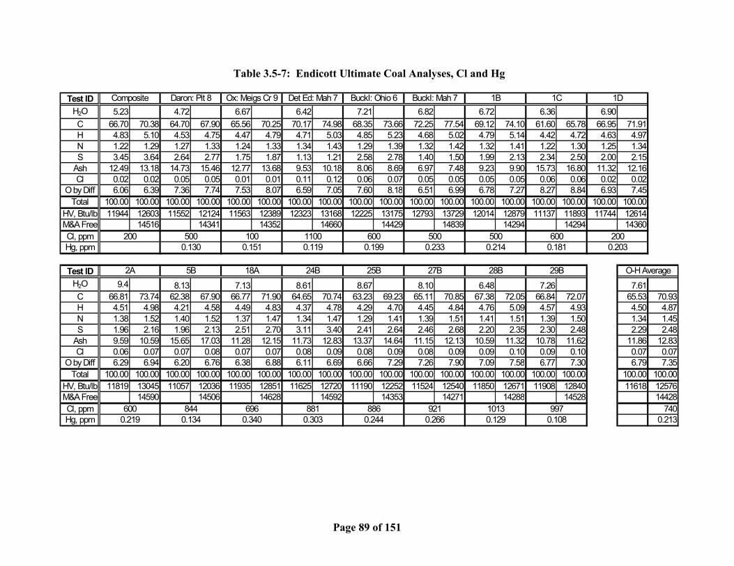
Page 89 of 151

Table 3.5-7: Endicott Ultimate Coal Analyses, Cl and Hg

Test IDH2O 5.23 4.72 6.67 6.42 7.21 6.82 6.72 6.36 6.90C 66.70 70.38 64.70 67.90 65.56 70.25 70.17 74.98 68.35 73.66 72.25 77.54 69.12 74.10 61.60 65.78 66.95 71.91H 4.83 5.10 4.53 4.75 4.47 4.79 4.71 5.03 4.85 5.23 4.68 5.02 4.79 5.14 4.42 4.72 4.63 4.97N 1.22 1.29 1.27 1.33 1.24 1.33 1.34 1.43 1.29 1.39 1.32 1.42 1.32 1.41 1.22 1.30 1.25 1.34S 3.45 3.64 2.64 2.77 1.75 1.87 1.13 1.21 2.58 2.78 1.40 1.50 1.99 2.13 2.34 2.50 2.00 2.15

Ash 12.49 13.18 14.73 15.46 12.77 13.68 9.53 10.18 8.06 8.69 6.97 7.48 9.23 9.90 15.73 16.80 11.32 12.16Cl 0.02 0.02 0.05 0.05 0.01 0.01 0.11 0.12 0.06 0.07 0.05 0.05 0.05 0.05 0.06 0.06 0.02 0.02

O by Diff 6.06 6.39 7.36 7.74 7.53 8.07 6.59 7.05 7.60 8.18 6.51 6.99 6.78 7.27 8.27 8.84 6.93 7.45Total 100.00 100.00 100.00 100.00 100.00 100.00 100.00 100.00 100.00 100.00 100.00 100.00 100.00 100.00 100.00 100.00 100.00 100.00

HV, Btu/lb 11944 12603 11552 12124 11563 12389 12323 13168 12225 13175 12793 13729 12014 12879 11137 11893 11744 12614M&A Free 14516 14341 14352 14660 14429 14839 14294 14294 14360Cl, ppmHg, ppm

Test IDH2O 9.4 8.13 7.13 8.61 8.67 8.10 6.48 7.26 7.61C 66.81 73.74 62.38 67.90 66.77 71.90 64.65 70.74 63.23 69.23 65.11 70.85 67.38 72.05 66.84 72.07 65.53 70.93H 4.51 4.98 4.21 4.58 4.49 4.83 4.37 4.78 4.29 4.70 4.45 4.84 4.76 5.09 4.57 4.93 4.50 4.87N 1.38 1.52 1.40 1.52 1.37 1.47 1.34 1.47 1.29 1.41 1.39 1.51 1.41 1.51 1.39 1.50 1.34 1.45S 1.96 2.16 1.96 2.13 2.51 2.70 3.11 3.40 2.41 2.64 2.46 2.68 2.20 2.35 2.30 2.48 2.29 2.48

Ash 9.59 10.59 15.65 17.03 11.28 12.15 11.73 12.83 13.37 14.64 11.15 12.13 10.59 11.32 10.78 11.62 11.86 12.83Cl 0.06 0.07 0.07 0.08 0.07 0.07 0.08 0.09 0.08 0.09 0.08 0.09 0.09 0.10 0.09 0.10 0.07 0.07

O by Diff 6.29 6.94 6.20 6.76 6.38 6.88 6.11 6.69 6.66 7.29 7.26 7.90 7.09 7.58 6.77 7.30 6.79 7.35Total 100.00 100.00 100.00 100.00 100.00 100.00 100.00 100.00 100.00 100.00 100.00 100.00 100.00 100.00 100.00 100.00 100.00 100.00

HV, Btu/lb 11819 13045 11057 12036 11935 12851 11625 12720 11190 12252 11524 12540 11850 12671 11908 12840 11618 12576M&A Free 14590 14506 14628 14592 14353 14271 14288 14528 14428Cl, ppm 740Hg, ppm 0.2130.219 0.134 0.340 0.303 0.244 0.266 0.129 0.108

886 921 1013 997600 844 696 881

2A 5B 18A 24B

0.181

25B 27B 28B 29B

600

O-H Average

2000.130 0.151 0.119 0.199 0.233 0.214

200 500 100 1100

Composite Daron: Pit 8 Ox: Meigs Cr 9 Det Ed: Mah 7 1DBuckI: Ohio 6 BuckI: Mah 7 1B 1C

0.203600 500 500

Page 90 of 151

Table 3.5-8: Endicott Coal: Cl, Hg

Test ID Hg Cl Test ID Hg Cl

ppm ppm ppm ppm

Composite 200 9A 0.313 799Pitt8 0.130 500 11A 0.148 787

MeigsCr9 0.151 100 13A 0.241 783DE-Mah7 0.119 1100 15A 0.349 795Ohio6A 0.199 600 18A 0.340 696BI-Mah7 0.233 500 20A 0.135 852

1B 0.214 500 22A 0.101 7751C 0.181 600 23B 0.230 8911D 0.203 200 24B 0.303 8812A 0.219 600 25B 0.244 8863B 0.247 906 26B 0.148 8314B 0.229 1037 27B 0.266 9215B 0.134 844 28B 0.129 1013

6B 0.134 1073 29B 0.108 9977B 0.370 799 30B 0.268 11198B 0.199 842 Standard 0.145 1108

Hg Std = 0.132 BCR182Cl Std = 1144 +/- 32 NIST 1630a

Table 3.5-9: Zimmer Ultimate Coal Analyses, Cl and Hg O-H Test ID 37 38 44 44Unload Date 10/17/01 10/21/01 10/21/01 10/29/01 10/30/01 11/5/01 11/5/01 11/11/01 11/11/01 11/19/01

Ash 12.04 10.06 9.52 9.98 11.75 14.47 10.97 14.16 12.34 9.50H 4.96 5.13 5.20 5.07 4.94 4.77 5.20 4.76 5.16 5.16C 68.93 72.34 72.38 72.81 68.93 66.45 72.36 67.01 71.29 73.45N 1.76 1.27 1.17 1.24 1.30 1.17 1.25 1.33 1.39 1.35S 4.28 4.01 4.39 4.10 3.73 4.79 4.09 3.90 3.75 4.10O 8.03 7.19 7.34 6.80 9.35 8.35 6.13 8.84 6.07 6.44

Total 100.00 100.00 100.00 100.00 100.00 100.00 100.00 100.00 100.00 100.00Cl, ppm 216 534 481 373 217 217 321 326 587 481Hg, ppm 0.24 0.13 0.11 0.12 0.21 0.18 0.10 0.14 0.15 0.10

Testing at Zimmer began 10/23/01 and ended 11/5/01

Page 91 of 151

Endicott Coal Analyses

0.00

0.05

0.10

0.15

0.20

0.25

0.30

0.35

0.40C

ompo

site

Pitt8

Mei

gsC

r9

DE-

Mah

7

Ohi

o6A

BI-M

ah7

1B 1C 1D 2A 3B 4B 5B 6B 7B 8B 9A 11A

13A

15A

18A

20A

22A

23B

24B

25B

26B

27B

28B

29B

30B

Hg,

ppm

0

150

300

450

600

750

900

1050

1200

Cl,

ppm

HgCl

Figure 3.5-25: Cl and Hg in Endicott Coal Samples

Zimmer Coal Analyses

0.00

0.05

0.10

0.15

0.20

0.25

0.30

0.35

0.40

10/1

7/01

10/2

1/01

10/2

1/01

10/2

9/01

10/3

0/01

11/5

/01

11/5

/01

11/1

1/01

11/1

1/01

11/1

9/01

Hg,

ppm

0

150

300

450

600

750

900

1050

1200

Cl,

ppm

HgCl

3837 44 44

Figure 3.5-26: Cl and Hg in Zimmer Coal Samples

Page 92 of 151

3.5.2 Thermal Dissociation Tests Results from conventional wet chemical analyses have shown that the mercury in wet scrubber exists in a form that is insoluble in water. Calculations also show that the mercury content in most coals is so low that, even if all the mercury ended up in the scrubber by products and in a soluble form, the sludge would pass the standard TCLP test used to characterize polutant leachability. Therefore, the purpose of this study was to determine the chemical form and thermal stability of mercury compounds in CUB. Normal wet chemistry and other analytical methods cannot be used to distinguish the various mercury compounds in CUB because they are present in very small amounts. However, most mercury analyzers are capable of detecting mercury at very low concentrations in gas streams. MTI developed a method whereby CUB are heated in an oven and the mercury in the off gas is continueously measured to generate a plot of mercury concentration versus temperature. Figure 3.5-27 shows vapor pressure curves for Hg0 and several simple mercury salts that may exist in CUB. The figure shows that different mercury compounds have significantly different vapor pressures at any given temperature. Theoretically, these differences could be used to determine what mercury compounds exist in CUB since the mercury compounds should vaporize at different rates and produce an off gas of varying concentration depending on the temperature. The discussion below describes the apparatus used in this study, how standards were prepared and tested and, finally, the results of TDT from Endicott and Zimmer samples and from previous TDT. In all, 33 TDT were conducted as part of this study.

Vapor Pressure of Hg and its Salts

1E-12

1E-11

1E-10

1E-09

1E-08

1E-07

1E-06

1E-05

0.0001

0.001

0.01

0.1

1

10

100

1000

0 50 100 150 200 250 300 350 400 450 500 550 600 650 700

Temperature, °C

Vapo

r Pre

ssur

e, a

tm.

Hgo

HgCl2

Range of partial pressure of mercury in flue gases from coal combustion

HgS

Minimum Risk Level, MRL

HgO

Figure 3.5-27: Vapor Pressure of Hg0 and Select Hg Salts

Page 93 of 151

3.5.2.1 Apparatus and Method A schematic of the TDT apparatus is shown in Figure 3.5-28 and photographs 3.5-29 through 3.5-33. It consists of an Argon source, an Argon flow meter, a temperature controlled tube furnace, a high temperature furnace, an impinger to convert all mercury to Hg0 (Figure 3.5-33), a chiller to remove water vapor, a PSA Mercury Analyzer (Figure 3.5-32) and a data acquisition system (Figure 3.5-30). Temperature is measured at the sample location (TC1), in the pyrolyzer (TC2), and at the junction of the pyrolyzer outlet and heated hose (TC3). Argon flow was held at 250 ml/min throughout the test. Test samples were placed in a glass sample boat (preheated to 800°C to purge mercury) and placed in the control oven (Figure 3.5-31). The samples were first heated to 95°C to evaporate all liquid water, then to 140°C to evolve the first waters of hydration from gypsum, and finally to 600°C at a rate of 6°C/min. The temperature of 140°C was chosen not to exceed the temperature at which the final waters of hydration evolve from the gypsum. This is the highest temperature that most CUBs are exposed to and is similar to the maximum temperature at a wallboard production plant. CaSO4·2H2O + Heat (128°C) CaSO4·½H2O + 1½ H2O + Heat (168°C) CaSO4 + ½H2O

Gases from the control oven then pass through the pyrolyzer and impinger to convert gaseous mercury compounds to elemental mercury. Mercury is then measured by atomic fluorescence in the PSA analyzer. For this application, the gold trap was bypassed so the detector would produce a continuous mercury signal.

Ar

FlowMeter

Control Oven Pyrolyzer

HgO

ImpingerChiller

TC 1 TC 2

Mercury CEM

SampleBoat

0-700°C 700°C

TC 3

Heated Hose 400°F

Figure 3.5-28: Thermal Dissociation Test Apparatus

Page 94 of 151

Figure 3.5-29: TDT Heated Hose, Pyrolyzer, Control Oven, Argon Flow Meters

Figure 3.5-30: TDT Data Acquisition System

Page 95 of 151

Figure 3.5-31: TDT, Inserting a Sample Boat into the Control Oven

Figure 3.5-32: PSA Mercury Analyzer and Preconditioner

Page 96 of 151

Figure 3.5-33: Hg0 Impinger

Page 97 of 151

Figure 3.5-34: Fines in Endicott Wet FGD Slurry

3.5.2.2 Preparation and Testing of Standards For this method to be successful it was important to develop and test standards made from pure mercury compounds in order to generate plots for comparison with CUB. It was beyond the scope of this study to test all the mercury compounds of interest, so several compounds were chosen based on the ions most likely to be found in the wet scrubber environment, namely mercuric chloride (HgCl2), mercuric sulfide (HgS), mercuric sulfate (HgSO4) and mercuric oxide (HgO). A blank, consisting of an empty sample boat, was also tested. To create the standards, the pure mercury compounds were ground and diluted with pure alumina to a target concentration of 1 ppm Hg. The alumina was prebaked at 800°C to drive off any mercury. The Thermal Dissociation Curve. Figure 3.5-35 shows the Thermal Dissociation Curve (TDC) produced by a typical TDT. This test represents the HgO Standard and will be used to explain the various features of the TDC. The title gives a description of the sample tested, its weight and the OH Test ID if applicable. The x-axis represents time and a typical TDC requires 2-3 hours to generate depending on the amount of time required to dry the sample before heating to 140°C. The left-hand y-axis shows control oven temperature in °C. The oven temperature curve,

Page 98 of 151

represented by the bold red line, shows that the sample was heated from room temperature to 95°C, held at 95°C for 5 min., heated at 6°C/min. to 140°C, held at 140°C for 10 min., then heated to 600°C at 6°C/min. The right-hand y-axis shows mercury concentration. No units are given because the software controlling the mercury analyzer was not written for the case in which the gold trap is bypassed as was done for this study. However, later in this section it will be shown that area under the mercury curve is equivalent to about 15 times the mercury measured by conventional methods in ppm. Furthermore, the most important information to be gleaned from the TDC is not the instantaneous mercury concentration but the temperature at which mercury is detected, the general shape of the mercury curve and the area under the curve. The right-hand y-axis also begins at ten instead of zero so that the background mercury value, another anomaly of operating the analyzer with the gold trap bypassed, is not shown. The conclusions from this figure are that a very small amount of mercury evolved at 140°C and the rest evolved and peaked at 300°C. It is also important to pay attention to the peak height and how it relates to the sample weight. For some samples, 0.01g produced peaks up to 550 indicating a high mercury concentration (wet FGD slurry fines), while 15g of other samples only produced peaks of 60 indicating very low mercury concentrations (Zimmer ESP ash). Therefore, peak heights cannot be directly compared unless sample weight is also considered. This TDC can now be compared with those produced from field test samples to see if there are similarities. Blank. Figure 3.5-36 shows the TDC for a blank sample boat. The result was that no mercury evolved during the test since the signal was below 10 for the entire test. This indicates there was no mercury contamination on the boat or in the system. Area vs. Concentration. Figure 3.5-37 shows the TDC for three sample weights of a HgSO4 Standard prepared and tested during a previous program. This figure is reproduced here to demonstrate how the area under the curve can be used as a relative measure of mercury concentration in the samples. The sample weights tested were equivalent to about 1x, 0.5x and 0.25x and corresponded well with the normalized areas under the curves of 0.999, 0.496 and 0.245. HgO Standard. Figures 3.5-38 and 3.5-39 show the TDCs for the HgO Standard from a test conducted in 20001 and one from the current project, respectively. These figures show good agreement between the two programs in that both curves were well defined and peaked at about 300°C. HgS Standard. Figures 3.5-40 and 3.5-41 show the TDCs for the HgS Standard from a test conducted in 20001 and one from the current project, respectively. These figures show good agreement between the two programs in that both curves were well defined and peaked at about 300°C. Unfortunately, both HgS and HgO produced TDC, as would be predicted by the vapor pressure curves in Figure 3.5-27, so that it would be difficult to distinguish between these compounds by this method if they were present in the field samples. HgSO4 Standard. Figures 3.5-42 and 3.5-43 show the TDCs for the HgSO4 Standard from a test conducted in 20001 and one from the current project, respectively. These figures both contain a minor peak at 300°C and a major peak at about 400°C. However, the TDC from 2002

Page 99 of 151

has a more pronounced minor peak and a major peak at 380°C compared to 425°C from the TDC of 2000. The explanation for this is not clear, but several improvements were made to the apparatus since the previous program that greatly improved the overall performance of the system. The peak at 380°C is also the highest for any material tested to date. HgCl2 Standard. Figures 3.5-44 and 3.5-45 show the TDCs for the HgCl2 Standard from a test conducted in 20001 and one from the current project, respectively. Although the figures appear different at first glance, they also have several similarities. First, both figures show some release of mercury at or below 140°C which the other standards do not. This is consistent with the vapor pressure curves in Figure 3.6-27 that show HgCl2 and Hg0 having similar vapor pressure characteristics. Both TDC also exhibit a peak near 250°C and one at 300°C, however the strengths of the two peaks are quite different. More tests would be required to determine the cause of these differences. It may be related to the difficulties in preparing standards by the method of dry dilutions where microgram size samples of pure compounds have to mixed and diluted by a factor of 1000. The overall conclusions from the standard tests show that HgO and HgS produce well defined TDC that peak at 300°C, HgSO4 produces multiple peaks with one at a much higher temperature than the other standards of about 400°C, and HgCl2 also produces multiple peaks with one at around 250°C which is lower than the other standards.

Standard-HgO0.1013g HgO @ 1ppm Hg in Al2O3

0

100

200

300

400

500

600

Tem

pera

ture

, °C

10

60

110

160

210

260

310

Hg

Con

cent

ratio

n

Oven TempHg

Figure 3.5-35: Example TDC

Page 100 of 151

Blank Sample Boat

0

100

200

300

400

500

600

700Te

mpe

ratu

re, °

C

10

20

30

40

50

60

70

80

Hg

Con

cent

ratio

n

Oven TempHg

Figure 3.5-36: Blank Sample Boat

Figure 3.5-37: Multiple TDC for the HgSO4 Standard at Various Sample Weights

HgSO4 - 0.2019, 0.1009, 0.0523g @ 1 ppm Hg in Al2O3250 ml/min Ar, 2% SnCl2 in 5% NaOH, 6°C/min

0

50

100

150

200

250

300

350

400

450

500

550

600

8:54

8:57

9:00

9:03

9:06

9:10

9:13

9:16

9:19

9:22

9:25

9:28

9:31

9:34

9:37

9:40

9:43

9:47

9:50

9:53

9:56

9:59

10:0

2

10:0

5

10:0

8

10:1

1

10:1

4

10:1

7

10/23/00

Ove

n Te

mpe

ratu

re, °

C

0

50

100

150

200

250

300

350

400

Hg

Con

cent

ratio

n

Data Clipped

Heating Curve

Areas = 0.969, 0.496, and 0.245

Temperatures may be shiftd due to sample boat position.

Page 101 of 151

HgO - 0.1567 g @ ~1 ppm Hg in Al2O3250 ml/min Ar, 2% SnCl2 in 5% NaOH, 6°C/min, Test: 110700-2

0

50

100

150

200

250

300

350

400

450

500

550

60013

:03

13:0

8

13:1

2

13:1

6

13:2

0

13:2

4

13:2

8

13:3

3

13:3

7

13:4

1

13:4

5

13:4

9

13:5

3

13:5

8

14:0

2

14:0

6

14:1

0

14:1

4

14:1

8

14:2

3

14:2

7

14:3

1

14:3

5

14:3

9

14:4

3

14:4

8

14:5

2

14:5

6

11/07/00

Ove

n Te

mpe

ratu

re, °

C

0

20

40

60

80

100

120

140

160

Hg

Con

cent

ratio

n

Area=0.390

Figure 3.5-38: TDC for the HgO Standard Year 2000

Standard-HgO0.1013g HgO @ 1ppm Hg in Al2O3

0

100

200

300

400

500

600

Tem

pera

ture

, °C

10

60

110

160

210

260

310

Hg

Con

cent

ratio

n

Oven TempHg

Figure 3.5-39: TDC for the HgO Standard Year 2002

Page 102 of 151

HgS - 0.1028 g @ ~1 ppm Hg in Al2O3250 ml/min Ar, 2% SnCl2 in 5% NaOH, 6°C/min, Test: 110700-4

0

50

100

150

200

250

300

350

400

450

500

550

60019

:15

19:1

9

19:2

2

19:2

6

19:3

0

19:3

4

19:3

8

19:4

2

19:4

5

19:4

9

19:5

3

19:5

7

20:0

1

20:0

5

20:0

8

20:1

2

20:1

6

20:2

0

20:2

4

20:2

8

20:3

1

20:3

5

20:3

9

20:4

3

20:4

7

20:5

1

20:5

4

20:5

8

11/04/00

Ove

n Te

mpe

ratu

re, °

C

0

20

40

60

80

100

120

140

160

Hg

Con

cent

ratio

n

Area=0.379

Figure 3.5-40: TDC for the HgS Standard Year 2000

Standard-HgS0.1077g HgS @ 1ppm Hg in Al2O3

0

100

200

300

400

500

600

Tem

pera

ture

, °C

10

60

110

160

210

260

310

Hg

Con

cent

ratio

n

Oven TempHg

Figure 3.5-41: TDC for the HgS Standard Year 2002

Page 103 of 151

HgSO4 - 0.0782 g @ ~1 ppm Hg in Al2O3250 ml/min Ar, 2% SnCl2 in 5% NaOH, 6°C/min, Test: 110700-3

0

50

100

150

200

250

300

350

400

450

500

550

60016

:44

16:4

8

16:5

2

16:5

6

17:0

0

17:0

4

17:0

8

17:1

2

17:1

6

17:2

0

17:2

4

17:2

8

17:3

2

17:3

6

17:4

0

17:4

4

17:4

8

17:5

2

17:5

6

18:0

0

18:0

4

18:0

8

18:1

2

18:1

6

18:2

0

18:2

4

18:2

8

18:3

2

11/07/00

Ove

n Te

mpe

ratu

re, °

C

0

10

20

30

40

50

60

70

80

90

100

Hg

Con

cent

ratio

n

Area=0.313

Figure 3.5-42: TDC for the HgSO4 Standard in 2000

Standard-HgSO40.7599g HgSO4 @ 1ppm Hg in Al2O3

0

100

200

300

400

500

600

Tem

pera

ture

, °C

10

85

160

235

310

385

460

Hg

Con

cent

ratio

nOven TempHg

Figure 3.5-43: TDC for the HgSO4 Standard in 2002

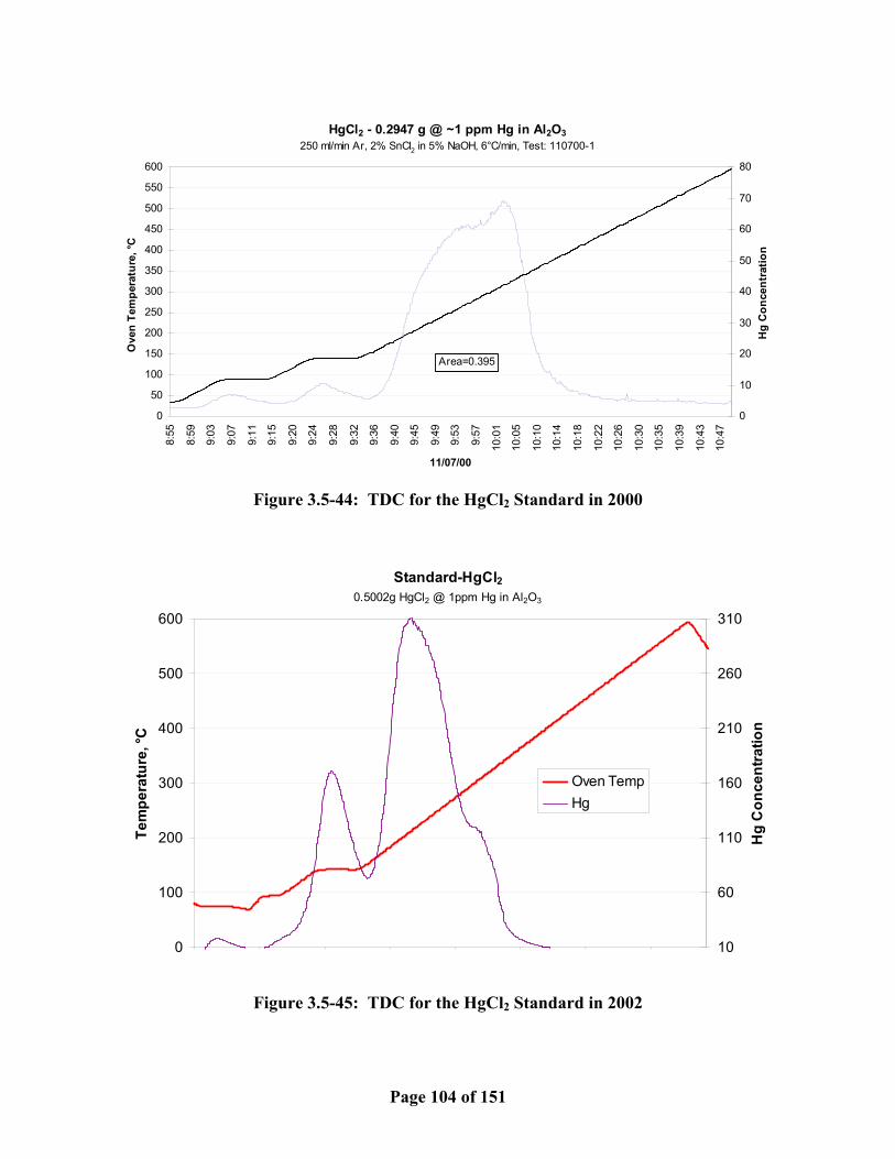
Page 104 of 151

HgCl2 - 0.2947 g @ ~1 ppm Hg in Al2O3250 ml/min Ar, 2% SnCl2 in 5% NaOH, 6°C/min, Test: 110700-1

0

50

100

150

200

250

300

350

400

450

500

550

6008:

55

8:59

9:03

9:07

9:11

9:15

9:20

9:24

9:28

9:32

9:36

9:40

9:45

9:49

9:53

9:57

10:0

1

10:0

5

10:1

0

10:1

4

10:1

8

10:2

2

10:2

6

10:3

0

10:3

5

10:3

9

10:4

3

10:4

7

11/07/00

Ove

n Te

mpe

ratu

re, °

C

0

10

20

30

40

50

60

70

80

Hg

Con

cent

ratio

n

Area=0.395

Figure 3.5-44: TDC for the HgCl2 Standard in 2000

Standard-HgCl20.5002g HgCl2 @ 1ppm Hg in Al2O3

0

100

200

300

400

500

600

Tem

pera

ture

, °C

10

60

110

160

210

260

310

Hg

Con

cent

ratio

nOven TempHg

Figure 3.5-45: TDC for the HgCl2 Standard in 2002

Page 105 of 151

3.5.2.3 TDT Tests of Endicott and Zimmer Samples This section presents TDT results for samples from both Endicott and Zimmer. Tables 3.5-3 and 3.5-4 show what samples were tested. A set of samples from the beginning (baseline) and end (steady state) of a test series was chosen to see if differences caused by the injection of the proprietary reagent could be ascertained. This section is organized into several parts comparing TDT data from Endicott and Zimmer for gypsum, ash, wet FGD slurry, wet FGD slurry fines and, finally, figures comparing TDT and conventional chemical analyses. Gypsum. The first two TDCs, Figures 3.5-46 and 3.5-47, represent gypsum from Endicott and Zimmer, respectively for baseline and steady state w/reagent injection. Both sets of curves show that there was a slight increase in mercury concentration between the two tests, but because of the variation in coal mercury content on a day-to-day basis, it is hard to attribute this solely to reagent injection. However, both sets of curves show that the gypsum contains a mercury compound that produces a peak at about 250°C. This is different than any of the standards except possibly HgCl2, but HgCl2 is soluble in water and was not detected in the liquid fractions of any of the samples so it is likely something different. The curves also show that a second compound may be present. For Zimmer, this is exhibited by the double peak, and in the Endicott samples it is exhibited by the slow rate of decay or large shoulder after the peak. Notice that the rate of decay after the peak is very sharp in the Zimmer curves in contrast to the Endicott curves. ESP Ash. Figure 3.5-48 is the TDC for Endicott ESP Ash for three fields and Figure 3.5-49 is the TDC for Endicott Waste Ash, which is a combination of economizer, air heater and ESP ash that has been wetted in a pug mill to reduce dust problems while loading into trucks for disposal. The results for Zimmer Ash are not presented because, as shown in section 3.5.2, this ash contained very little mercury and 15 grams of sample barely produced peaks above the background level. The TDCs for the Endicott Ash show several things. First, the ESP ash contained a mercury compound that produced peaks between 360-400°C. This is somewhat consistent with the HgSO4 standard but the shapes of the curves are very different. Secondly, the ash in the latter fields appear to contain a second mercury compound with a much lower peak temperature of about 220°C. This peak is barely present in the Field 1 sample, grows stronger in the Field 2 and becomes distinctly pronounced in Field 3. This suggests that different mercury compounds may be present depending on the make up of the ash collected in each field. Finally, the waste ash, a combination of economizer, air heater and ESP ash, produced a surprisingly different TDC than the ESP ash with a peak temperature of only about 280°C. However, it was sampled after being wetted in the pug mill to control dusting. It is known that HgSO4 breaks down in water and may form HgS or HgO which is consistent with the TDCs. Wet FGD Slurry. Figures 3.5-50 and 3.5-51 show the TDCs for wet FGD slurry solids from Endicott and Zimmer respectively. The three curves in each figure represent a baseline, steady state, and a dried sample. A dried sample, dried overnight at 95°F, was tested to determine if drying affected the TDC. It is much easier to test dried samples since much smaller amounts are needed and there is no need for lengthy drying times before heating to 140°C. The curves show a significant difference between Endicott and Zimmer, which is not unexpected since Zimmer uses Thiosorbic Lime and natural oxidation in the scrubber, whereas Endicott is a conventional limestone forced oxidation system. The Zimmer slurry produced two distinct peaks, a main peak

Page 106 of 151

at about 220°C and a minor peak at about 400°C. In contrast, the Endicott slurry produced several small peaks at or below 140°C, a main peak at about 280°C and a smaller shoulder peak at about 350°C that was followed by a gradual decay. Drying had no apparent effect on the samples. The TDCs produced by the slurry are different than those produced by the gypsum. This can be explained for Zimmer since the slurry is subjected to a multistage chemical process in the ex situ oxidation system. However, the slurry at Endicott is simply pumped to a thickener and the underflow is sent to filter drums to separate the gypsum. There are other streams added to the thickener, like the material from the scrubber building sumps, so some additional chemical reactions may occur.

Endicott - Gypsum0.9959g Test 050901-1B

1.1025g Test 071001-21A

0

100

200

300

400

500

600

Tem

pera

ture

, °C

10

120

230

340

450

560

670

Hg

Con

cent

ratio

n

Oven TempTest-1BTest-21A

Figure 3.5-46: TDC for Endicott Gypsum

Page 107 of 151

Zimmer - Gypsum10.01g Test 102501-33A 10.21g Test 110101-39A

0

100

200

300

400

500

600

Tem

pera

ture

, °C

10

210

410

610

810

1010

1210

Hg

Con

cent

ratio

n

Oven TempTest-33ATest-39A

Figure 3.5-47: TDC for Zimmer Gypsum

Endicott - ESP Ash2.21g Field 1 Hopper 12 - Test 071001-21A

0.266g Field 2 Hopper 11 - Test 071001-21A1.50g Field 3 Hopper 10 - Test 071001-21A

0

100

200

300

400

500

600

Tem

pera

ture

, °C

10

130

250

370

490

610

730

Hg

Con

cent

ratio

nOven Temp

Field1

Field2

Field3

Figure 3.5-48: TDC for Endicott ESP Ash by Field

Page 108 of 151

Endicott - Waste Ash3.11g Test 050901-1B

2.95g Test 071001-21A

0

100

200

300

400

500

600

Tem

pera

ture

, °C

10

70

130

190

250

310

370

430

Hg

Con

cent

ratio

n

Oven TempTest-1BTest 21A

Figure 3.5-49: TDC for Endicott Waste Ash

Endicott - WFGD Slurry 3.17g Test 050901-1D

2.90g Test 071001-21A 0.584g Test 071001-21A(dry)

0

100

200

300

400

500

600

Tem

pera

ture

, °C

10

50

90

130

170

210

250

Hg

Con

cent

ratio

n

Oven TempTest-1DTest-21ATest-21A(dry)

Figure 3.5-50: TDC for Endicott Wet FGD Slurry

Page 109 of 151

Zimmer - WFGD Slurry 2.73g Test 102501-33A 2.87g Test 110101-39A

0.498g Test 110101-39A(dry)

0

100

200

300

400

500

600

Tem

pera

ture

, °C

10

70

130

190

250

310

370

Hg

Con

cent

ratio

n

Oven TempTest-33ATest-39ATest-39A(dry)

Figure 3.5-51: TDC for Zimmer Wet FGD Slurry Wet FGD Slurry Fines. Figures 3.5-52 and 3.5-53 show the TDCs for wet FGD slurry fines from Endicott and Zimmer respectively. Slurry fines are separated from the gypsum product and disposed separately at Zimmer (Figure 3.5-19). At Endicott, the fines build up in the slurry until they are removed with the gypsum on the filter drums. To get a sample of the fines from Endicott, a slurry sample was mixed, and then allowed to stand until only the white gypsum portion settled. The liquid above the white layer was still black at this point from the suspended fines. This dark liquid was drawn off, filtered, and dried overnight at 95°F. Figure 3.5-34 shows the dark, fine layer on a completely settled sample of scrubber slurry from Endicott. The Endicott fines produced a single, well defined peak at about 240°C. This is consistent with the major peak in both the gypsum and the slurry and is, therefore, the likely source for most of the mercury in these samples. Note that only 0.01 g of this material produced a peak over 500 whereas 0.58 g of the dried slurry only produced a peak of 250 which means the mercury is heavily concentrated in the fines. The same holds true for the Zimmer fines except that the peak temperature is about 250°C and the mercury concentration is a bit lower as compared to the slurry. However, the separation method employed at Zimmer is not as discriminating as what was done in the lab. Water Treatment Sludge. Figure 3.5-54 shows the TDC for the water treatment sludge solids from Endicott. Water treatment sludge is a material produced at Endicott in the water treatment plant. It is pumped to the wet scrubber to take advantage of its high alkalinity. All waste water streams at Endicott are pumped to the plant and undergo a multistage process including

Page 110 of 151

acidification, precipitation, clarification, and neutralization, before being discharged. The sludge from the neutralization step overflows a weir in the bottom of a tank (Figure 3.5-7) and is periodically pumped to the wet scrubber. This stream was sampled because it is a possible source of mercury to the system, and the solids were found to contain about as much mercury as the wet FGD slurry solids (Table 3.5-5). However, the flow rate of this stream is very small and so it is not a main source of mercury. The TDC for this material shows two peaks, a major peak at about 260°C and a minor peak at 380°C. The material from the earlier test (Test 1A) also had a peak at about 330°C. The two main peaks look very similar to those produced by the wet FGD slurry from Zimmer which suggests that the two materials contain the same mercury compounds or compounds with similar vapor pressures.

Endicott - WFGD Slurry Fines0.0108g Test 090501-27B(dry)

0

100

200

300

400

500

600

Tem

pera

ture

, °C

10

110

210

310

410

510

610

Hg

Con

cent

ratio

n

Oven TempTest 27B(dry)

Note that a very small amount of sample produced a very large mercury peak.

Figure 3.5-52: TDC for Endicott Wet FGD Slurry Fines

Page 111 of 151

Zimmer - Fines from Centrifuge0.274g Test 102501-33A0.250g Test 110101-39A

0

100

200

300

400

500

600

Tem

pera

ture

, °C

10

140

270

400

530

660

790

Hg

Con

cent

ratio

n


Figure 3.5-53: TDC for Zimmer Wet FGD Slurry Fines

Endicott - Water Treatment Sludge0.236g Test 050801-1A(dry)

0.846g Test 071001-21A(dry)

0

100

200

300

400

500

600

Tem

pera

ture

, °C

10

70

130

190

250

310

370

Hg

Con

cent

ratio

n


Figure 3.5-54: TDC for Endicott Water Treatment Sludge

Page 112 of 151

3.5.2.4 TDT vs. Conventional Chemistry Figures 3.5-55 through 3.5-57 present a comparison of TDT data and conventional chemical analyses. To generate these plots, the area under the TDC was calculated by:

Area = (∫((Hgn-10 + Hgn+1-10)/2*∆t)))/wt/1000 Where:

Hg ≡ mercury concentration measured by the PSA analyzer, n ≡ the number assigned to each Hg value measured, ∆t ≡ time interval between n and n+1 (∆t = 5 sec for this study), wt ≡ dry sample weight in grams This equation states that the average value between two successive outputs from the mercury analyzer is multiplied by the time interval and summed over the entire length of the test, and the sum is then divided by the sample weight and by 1000. A value of 10 was subtracted from each output to nullify the background signal. The sum was divided by 1000 simply to produce values for the area that were in a reasonable range. Figure 3.5-55 shows the TDT Area plotted on the right-hand y-axis and the Hg concentration from conventional chemical analyses on the left-hand axis for the ESP and waste ash samples from Endicott and Zimmer. The data is further separated into columns representing the particular field the sample came from. This figure shows that there is good agreement between the two methods and that further dividing the TDT Area by 15 would produce a value equivalent to the ppm values for the conventional analyses. It further shows that the TDT correctly distinguished between the relatively high mercury in the Endicott ash compared to the Zimmer ash. Figure 3.5-56 is a similar comparison for the slurry and gypsum samples. Again, there is good agreement between the two methods when the TDT areas are factored by 15. The TDC area method again correctly indicated the low mercury levels in the Zimmer Gypsum as compared to other samples. Finally, Figure 3.5-57 shows the same comparison for the wet FGD slurry fines, which contained the highest mercury concentration of any of the samples tested. This figure shows that there is good agreement between the methods for the Zimmer Fines, but no conventional chemical analyses were performed on the Endicott fines. Therefore, a one-to-one comparison shows that converting the TDT area to ppm yields a value for the Endicott fines of about 38 ppm Hg. This is about twice as high as the Zimmer fines and much higher than the Endicott gypsum values of 1 ppm Hg, but it is consistent with what was seen for the Zimmer samples. There are two important conclusions from the TDT study. First, it confirmed, for two very different plants, that the mercury captured by wet scrubbers is not bound with the larger gypsum crystals but is present as a separate, fine particulate or is bound to other fine particulate in the slurry. This suggests that the mercury captured by wet scrubbers can be separated from the gypsum product by adding a step to separate the fines. The fines can then be disposed properly.

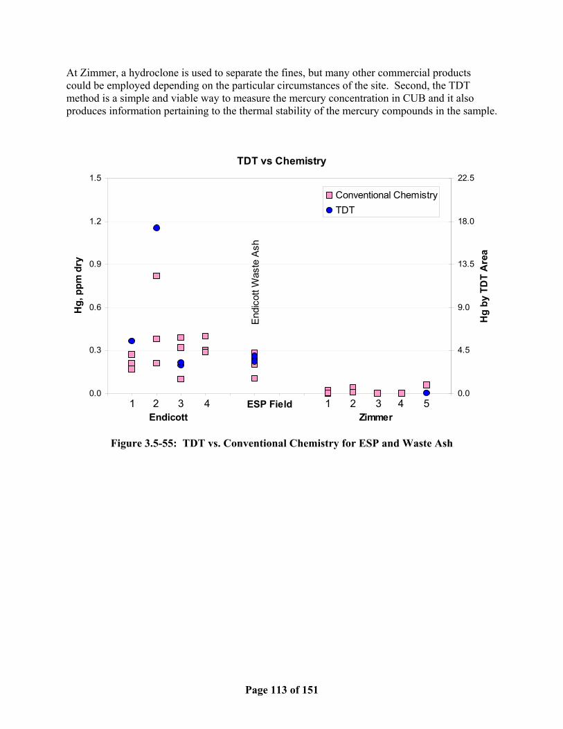
Page 113 of 151

At Zimmer, a hydroclone is used to separate the fines, but many other commercial products could be employed depending on the particular circumstances of the site. Second, the TDT method is a simple and viable way to measure the mercury concentration in CUB and it also produces information pertaining to the thermal stability of the mercury compounds in the sample.

TDT vs Chemistry

0.0

0.3

0.6

0.9

1.2

1.5

Hg,

ppm

dry

0.0

4.5

9.0

13.5

18.0

22.5

Hg

by T

DT

Are

a

Conventional ChemistryTDT

Endicott ZimmerESP Field 1 2 3 4 51 2 3 4

Endi

cott

Was

te A

sh

Figure 3.5-55: TDT vs. Conventional Chemistry for ESP and Waste Ash

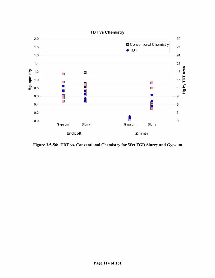
Page 114 of 151

TDT vs Chemistry

0.0

0.2

0.4

0.6

0.8

1.0

1.2

1.4

1.6

1.8

2.0

Hg,

ppm

dry

0

3

6

9

12

15

18

21

24

27

30

Hg

by T

DT

Are

a


Endicott Zimmer

Gypsum Slurry Gypsum Slurry

Figure 3.5-56: TDT vs. Conventional Chemistry for Wet FGD Slurry and Gypsum

Page 115 of 151

TDT vs Chemistry

0

5

10

15

20

25

30

35

40

Hg,

ppm

dry

0

75

150

225

300

375

450

525

600

Hg

by T

DT

Are

a


EndicottZimmerFines Fines

Figure 3.5-57: TDT vs. Conventional Chemistry for Wet FGD Slurry Fines

Page 116 of 151

3.5.3 Mercury Tracking Data from the chemical analyses and OH results were combined with flow rate data for the various streams to determine what the major sources of mercury input and output were for Zimmer and Endicott. It should be noted that it was never a goal of this project to obtain the data and samples required to do a thorough mercury mass balance for the plants. The purpose of this section is to depict how the mercury transits through the plants. Several assumptions were made to perform the analysis presented below because several of the major process stream flow rates are not measured directly. Therefore, flow rate data was obtained from various sources including mass balance flow sheets, conversations with plant personnel, combustion calculations and the plants’ data acquisition system. Gas flow rates were determined from in-house combustion calculations and were based on average coal compositions of samples taken during this program and on the knowledge of plant personnel concerning normal coal consumption. All calculations were done assuming full-load operation even though both plants cycled during the test period. The fly ash split between the air heater/economizer and the ESP was assumed to be 20:80 and the ash in the air heater/economizer was assumed to contain no mercury due to the high temperature at these locations. Many of the temperatures, pressures and flow rates were acquired during the project from the plant data acquisition systems as shown in Appendix B. Figure 3.5-58 shows the Hg flow schematic for Endicott. The overall mercury balance, based on total inlet and outlet mercury flow rates, was 105% (4.80 g/hr in/4.56 g/hr out*100%) which is very good considering all the assumptions that were made. The overall system removal based on the mercury in the coal and in the stack gas was 78% [(4.80 g/hr -1.06 g/hr)/4.80 g/hr*100%]. However, there is a discrepancy in that the coal mercury and ash mercury do not equate with the Wet FGD inlet mercury (4.80 g/hr - 1.60 g/hr ≠ 4.61 g/hr). This demonstrates the difficulty associated with doing this type of analysis and the danger in reading too much into the information. The most important thing to learn from the flow diagram is that, for Endicott, the largest source of mercury entering the system is the coal and that mercury exits the system in about equal parts with the fly ash, stack gas and gypsum. Figure 3.5-59 shows the Hg flow schematic for Zimmer. The overall mercury balance is fairly good at 83%. However, as with Endicott, the mercury entering the system with the coal does not equate with ash and flue gas mercury values (63.89 g/hr - 0.71 g/hr ≠ 83.29 g/hr). Calculating the overall system mercury removal based on these numbers does not make sense because the scrubber removal would be much greater than the overall removal. In this instance, it is best to assume that the overall system mercury removal is equal to the scrubber removal since scrubber removal is based on the OH measurements whereas the coal mercury is based on several assumptions about load, flows, etc. Also, since little mercury was measured in the ESP ash, the contribution of the ESP can be ignored. Based on this, the overall system mercury removal for Zimmer was 54% [(83.29 g/hr -38.2 g/hr)/83.29 g/hr*100%]. More importantly, the schematic shows that, contrary to Endicott, at Zimmer, most of the mercury exits the system with the stack gas and slurry fines. The fly ash and gypsum streams contain little mercury.

Page 117 of 151

Endicott Power StationMercury Flow Diagam Water

0.00Total Balance Hg, g/hrHg In = 4.80 g Hg/hrHg Out = 4.56 g Hg/hr

105 % (in/out) Water Treatment Sludge

Gas Gas Gas4.61 1.06

Air Hg, g/hr Hg, g/hr

GypsumCoal 1.904.80 Lime Slurry Hg, g/hr

Hg, g/hr 0.004Hg, g/hr

ESP Ash Water1.60

Hg, g/hr

Boiler

ESPScrubber

Thickener

Water Treatment Plant

Filter Drum

Stack

To WFGD or WTP

Figure 3.5–58: Hg Flow Schematic for Endicott

Page 118 of 151

Zimmer Power StationMercury Flow Diagram Water/Solids

0.50Total Balance Hg, g/hrHg In = 64 g Hg/hrHg Out = 77 g Hg/hr Fines

83 % (in/out) 33.42Hg, g/hr

Gas Gas Gas83.29 38.20

Air Hg, g/hr Hg, g/hr

Gypsum4.65

Coal Lime Slurry Hg, g/hr63.89 0.50

Hg, g/hr Hg, g/hrESP Ash Water

0.71Hg, g/hr

Boiler

ESPScrubber

Hydroclone

Centrifuge

Filter Belt

Stack

Reclaim WaterOxidizer

Thickener

-

Figure 3.5-59: Hg Flow Schematic for Zimmer

Page 119 of 151

3.5.4 CUBs Results and Conclusions 1. One of the most significant findings of the demonstration is that the mercury in the wet

FGD Slurry was associated with the fines. This is significant because the two plants represent opposite ends of the spectrum in plant size and wet scrubber chemistry, and yet both exhibited this behavior, as did the MTI Pilot in previous studies1. It is also important because the fines can be separated from the larger gypsum crystals through the addition of a variety of commercially available equipment to produce a gypsum product similar to natural gypsum as shown in the table below. The fines can be disposed in standard landfills because the mercury is in a stable form. This finding also suggests that the mercury in wet FGD CUB is not bound to gypsum and may be forming a fine particulate of a pure compound or reacting with some component of the fines, like soot.

Average Zimmer Endicott Natural Gypsum FGD Gypsum (w/o fines) (with fines) Minimum: 0.006 ppm (by wt) 0.03 0.03 0.48 Maximum: 0.05 ppm 1.32 0.10 1.15 From EPRI Technical Report2 TR-103652 2. The table below shows the averaged mercury concentrations for the major process streams.

The important differences include the low mercury content in the Zimmer ESP Ash and Gypsum. The low mercury in the ash may be due to the low amount of unburned carbon in the Zimmer Ash (1%) compared to Endicott Ash (9%). The gypsum has low mercury because it is separated from the fines as part of the process. The fines are not separated at Endicott, so to obtain the value shown below, the fines were separated in the lab. The mercury (and chlorine) in the coal varied by about a factor of three over the course of the test at both sites.

Hg, ppm(dry) Endicott Zimmer

Coal 0.21 0.15 ESP Ash 0.32 0.016 Gypsum 0.70 0.055


3. There was no significant mercury detected in any of the liquid fractions of the CUB, except

the Zimmer Centrifuge Water that was not filtered and may have contained fines. This indicates that HgCl2 is not one of the components in CUB because HgCl2 has an appreciable solubility in water.

4. The mercury content of the ESP Ash was not a strong function of ESP Field for the

samples that were tested. That is, the mercury was evenly distributed between the fields and did not concentrate with the particulate fines in the latter fields as might be expected. One explanation for this may be that the unburned carbon content in the ash also decreased

Page 120 of 151

in the latter fields at both sites. This would indicate that the unburned carbon is contained in a relatively coarse fraction of the ash or that very little material collected in the latter fields.

5. The Thermal Dissociation Test method using the mercury analyzer appears to be a viable

way of detecting small amounts of mercury in CUB. The method produced distinct concentration vs. temperature curves for several pure mercury compounds that correlate well to vapor pressure data for these compounds. However, the curves for HgS and HgO overlap each other which make them indistinguishable. The area under the dissociation curve was shown to be directly proportional to the mercury concentration measured by conventional chemical analysis. Refinements to the technique would require further standard development with other mercury compounds, more tests on a wider range of process samples and the development of a calibration technique for the analyzer.

6. The TDT for all samples showed three distinct sets of peaks clustered around 250, 300 and

400°C. Small differences may be due to changes in argon flow rate, sample boat position, etc., although these were held as constant as possible. The 300°C peak may correspond to HgSO4 since it only appeared in the dry ash samples and HgSO4 decomposes in water. The 300°C peak may correspond to HgS or HgO but these cannot be distinguished by this technique. The 250°C peak may be HgCl2, but it is unlikely since it is water soluble and no mercury was detected in the liquid fractions. It is more likely that this represents a compound that has not yet been tested as a standard.

7. All the CUB tested by TDT were stable below 140°C in that no significant amount of Hg

was released at or below 140°C. This is significant because it demonstrates that mercury will not be re-released into the environment through subsequent reprocessing of wet FGD CUB.

8. The TDT for Gypsum from Endicott and Zimmer had similar major peaks at about 250°C

with other minor peaks near the major peak. The proportion or composition of the various compounds may be different since the overall curves are distinctly different.

9. The TDT for ESP ash from Endicott had a major peak near 400°C, and ash from the latter

fields also had a minor peak near 250°C that indicates a different mercury compound in the particulate fines. The major peak shifted to 300°C after the ash had been mixed with water in the pug mill. This may represent the decomposition of HgSO4 in water. The Zimmer ESP Ash contained almost no mercury so its TDC was hard to distinguish from the background.

10. The TDT for wet FGD slurry from Endicott and Zimmer produced distinctly different

curves. Endicott slurry had a major peak at 300°C and some minor peaks between 300 and 400°C. Zimmer slurry produced a very sharp major peak at 250°C and a distinct minor peak at 400°C. It is interesting to note the after treatment in the ex situ oxidation system, the Zimmer gypsum produced a TDC very similar to Endicott suggesting that the chemical composition of the mercury compounds changed in the oxidation process.

Page 121 of 151

11. The TDT for wet FGD slurry fines from Endicott and Zimmer produced nearly identical peaks at about 250°C. The area under the curves, when correlated with conventional mercury analyses, showed that the fines contained the highest mercury concentration of any material yet tested at 38 ppm for Endicott and 13 ppm for Zimmer.

12. By correlating the average mercury concentrations measured in the various streams with

the average flow rates of those streams, it was determined that the major source of egress for mercury at Endicott is about equally split between the ESP ash, gypsum and stack gas, whereas the mercury at Zimmer mostly exits via the slurry fines and flue gas.

3.6 QUALITY ASSURANCE/QUALITY CONTROL General The objective of the MTI Research and Development Division (R&DD) quality management system is to ensure that the project work meets the intended R&D objective and can be understood and if necessary reproduced successfully by others. Work performed under this project by MTI was conducted in accordance with the R&DD STANDARD PRACTICE Quality Program. The R&DD STANDARD PRACTICE quality assurance program is well recognized as an outstanding base quality program for research work by such organizations as the U.S. DOE, U.S. DOD, EPRI, Gas Research Institute and many others and is the baseline operating level designation for normal business practices within R&DD. The program is specified in the Quality Management Manual and implemented by the Standard Practice Manual. The project workscope was defined by way of project planning with the result being an agreement with the customer at the outset of the project. Any changes to the workscope were also agreed upon with the customer. Accordingly, project records were maintained throughout the testing program to provide a historical account of all significant activities. The calibration of all measurement standards and measuring and test equipment used within the R&DD is controlled in order to ensure that measurements made are quantifiable and reproducible in terms of nationally recognized standards. The Quality Assurance organization exercises general surveillance over projects conducted according to STANDARD PRACTICE. An EPA and an internal audit, conducted to verify the implementation and effectiveness of the internal quality system, were performed during the course of this program; no findings which would affect the quality of the program data were reported. Project records are available for customer review at the R&DD. The retention of these records is in accordance with MTI policy (minimum five years) or as specified by customer requirements, applicable codes, standards or specifications.

Page 122 of 151

Instrument Calibration Instrument calibration procedures follow established, documented MTI R&DD Technical Procedures to ensure the sampling and process measurement equipment is functioning properly and the measurements can be traced to a known, defined standard. Instrumentation is generally certified on an annual basis. All of the instrumentation used to acquire test data during this program was required to have current certification. Certified instrumentation included all pressure transmitters, flow meters, dry gas meters, stopwatches and balances. The data acquisition system was certified to assure that the signals from the various instruments were properly transmitted to the storage system. The flue gas analyzers were regularly calibrated using NIST traceable standards throughout the test program. Sample Custody The chain of custody for the Ontario Hydro flue gas impinger samples was straightforward and effective. The glassware preparation team signed the glassware set-up data sheets when the sample trains were ready for use. The sampling crew then signed out the impinger train components when they were taken from the laboratory to the sampling site and signed them back in when they were returned to the lab. The sample sheets identified the sampler, sample location, sample method, test ID, filter holder number and glassware set. Laboratory Analysis The following methods were used to document the analytical and control procedures used in analysis of samples from operation of the test facility: • The procedures for the preparation of all reagents and materials that are used for the

collection of samples are documented in MTI Technical Procedures based on the EPA and Ontario Hydro Methods. Standardized sample forms are used to document the conditions under which all samples are collected along with identification of the persons responsible for the collection of the samples.

• All field recoveries, extractions, preservations and observations were documented on either

a standard form or in a bound laboratory notebook along with identification of the field analyst performing the sample handling.

• Pre-prepared sample container labels were affixed to all collected samples identifying the

time, date, sample location, project name, project charge number, sample method, and person responsible for sample recovery. An established laboratory sample numbering and tracking system was used to control the samples. Sample inventory sheets were used to account for the storage of all samples.

Page 123 of 151

The analytical QC effort focuses on ensuring the usefulness of the data generated. Standard EPA or ASTM analytical procedures are followed. The analytical QC procedures include a variety of internal QC checks designed to access and control the data quality as it is generated. The various QC checks, typical frequency and general acceptance criteria are summarized in Table 3.6-1. MDL refers to the method detection limits. The samples are usually analyzed in batches of 10 to 12 samples.

Table 3.6-1: Analytical Quality Control Checks for Trace Metal Analysis

QC Check

Frequency

Acceptance Criteria

Initial Calibration blank & Standards

Once per run

Not applicable

Calibration Verification (AA)

Every hour

% D ≤ 15%

Continuing Calibration Blank

With each calibration

Not applicable

Laboratory Control sample

Once per run

% D ≤ 20%

Matrix Blank

Once / matrix type

Not applicable

Spiked Sample

Once / matrix type

% R = 50 - 150%

3.7 TECHNICAL CONCLUSIONS 3.7.1 Ontario Hydro Flue Gas Sampling Conclusions Full-scale field demonstration testing was performed at two power plants to evaluate B&W/MTI’s advanced mercury control technology. The Ontario Hydro flue gas sampling method, designed to determine mercury speciation in the flue gas, was used to measure mercury concentration in the flue gas at the inlet and outlet of the wet FGD systems at both plants. Parametric tests, designed to establish feed rate/performance curves were performed at MSCPA’s Endicott station. Based on the results of the Parametric tests, Verification and Long Term tests, designed to show prolonged, reliable mercury removal performance with minimal impact on SO2 removal performance, were conducted. Average mercury removal across the wet FGD system during the Verification and Long Term tests ranged from 76% to 79%. Most of the oxidized mercury present in the flue gas was removed in the wet FGD system; no increase in

Page 124 of 151

elemental mercury concentration was observed during the Endicott testing, indicating that the control technology was successful in not only maintaining high oxidized mercury removal but simultaneously suppressing mercury reemission. Following the Endicott test program, two weeks of Verification tests were performed at Cinergy’s Zimmer station. Mercury removal across the wet FGD system during these tests averaged 51%. Compared to the Endicott results, lower oxidized mercury removal performance was observed at Zimmer (87% vs. 96%). In addition, elemental mercury concentrations increased across the wet FGD system, indicating that the control technology was not effective in suppressing the reemission of captured mercury from the scrubber. Testing conducted with 50% more reagent feed at the end of the Zimmer test program showed no improvement in mercury removal performance. At both power plants, the wet FGD systems were very effective in removing oxidized mercury from the flue gas entering the scrubber. Total wet FGD mercury removal performance, however, was limited by the amount of elemental mercury present in the inlet flue gas. A comparison of various technical scenarios illustrated the importance of a viable mercury oxidation technology in obtaining high total wet FGD mercury removals. In one example (75% oxidized, 25% elemental entering a wet FGD system), combining a viable oxidation technology with B&W/MTI’s control technology could improve mercury removal to 91%; by comparison, either technology by itself yielded a maximum removal of 78%. 3.7.2 Mercury in Coal Utilization By-Products Conclusions One of the most significant findings of the demonstration is that the mercury in the wet FGD Slurry was associated with the fines. This is significant because the two plants represent opposite ends of the spectrum in plant size and wet scrubber chemistry, and yet both exhibited this behavior, as did the MTI Pilot in previous studies1. It is also important because the fines can easily be separated from the larger gypsum crystals through the addition of a variety of commercially available equipment to produce a gypsum product similar to natural gypsum as shown in the table below. The fines can be disposed of in standard landfills because the mercury is in a stable form. This finding also suggests that the mercury in wet FGD CUB is not bound to gypsum and may be forming a fine particulate of a pure compound or reacting with some component of the fines, like soot. Average Zimmer Endicott Natural Gypsum FGD Gypsum (w/o fines) (with fines) Minimum: 0.006 ppm (by wt) 0.03 0.03 0.48 Maximum: 0.05 ppm 1.32 0.10 1.15 From EPRI Technical Report2 TR-103652 The table below shows the averaged mercury concentrations for the major process streams. The important differences include the low mercury content in the Zimmer ESP Ash and Gypsum. The low mercury in the ash may be due to the low amount of unburned carbon in the Zimmer Ash (1%) compared to Endicott Ash (9%). The gypsum has low mercury because it is separated

Page 125 of 151

from the fines as part of the process. The fines are not separated at Endicott, so to obtain the value shown below, the fines were separated in the lab. The mercury in the coal varied by about a factor of three over the course of the test at both sites.

Hg, ppm(dry) Endicott Zimmer Coal 0.21 0.15

ESP Ash 0.32 0.016 Gypsum 0.70 0.055


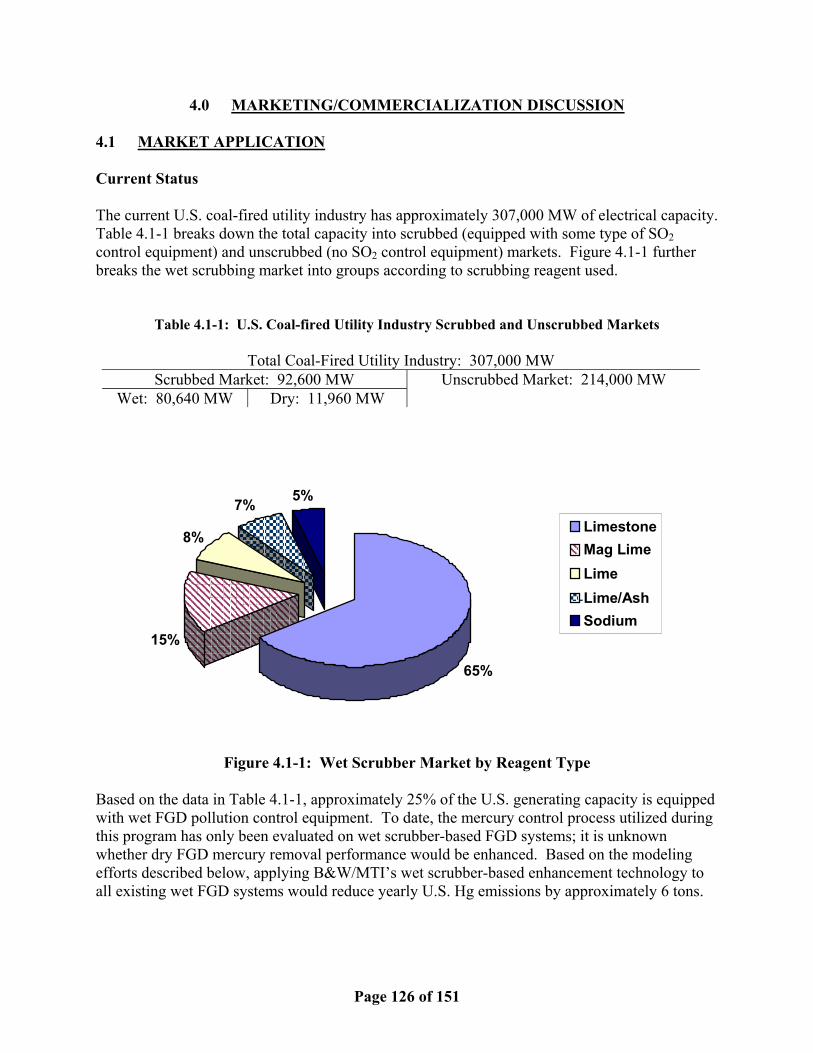
Page 126 of 151

4.0 MARKETING/COMMERCIALIZATION DISCUSSION 4.1 MARKET APPLICATION Current Status The current U.S. coal-fired utility industry has approximately 307,000 MW of electrical capacity. Table 4.1-1 breaks down the total capacity into scrubbed (equipped with some type of SO2 control equipment) and unscrubbed (no SO2 control equipment) markets. Figure 4.1-1 further breaks the wet scrubbing market into groups according to scrubbing reagent used.

Table 4.1-1: U.S. Coal-fired Utility Industry Scrubbed and Unscrubbed Markets

Total Coal-Fired Utility Industry: 307,000 MW Scrubbed Market: 92,600 MW

Wet: 80,640 MW Dry: 11,960 MW Unscrubbed Market: 214,000 MW

Figure 4.1-1: Wet Scrubber Market by Reagent Type

Based on the data in Table 4.1-1, approximately 25% of the U.S. generating capacity is equipped with wet FGD pollution control equipment. To date, the mercury control process utilized during this program has only been evaluated on wet scrubber-based FGD systems; it is unknown whether dry FGD mercury removal performance would be enhanced. Based on the modeling efforts described below, applying B&W/MTI’s wet scrubber-based enhancement technology to all existing wet FGD systems would reduce yearly U.S. Hg emissions by approximately 6 tons.

65%

15%

8%

7% 5%

LimestoneMag LimeLimeLime/AshSodium

Page 127 of 151

Future Impact B&W previously developed a model of the impact of enhanced wet FGD mercury emissions control based on a detailed coal-fired utility database, data from US EPA’s ICR effort and published emission factors, and data obtained during the mercury control technology evaluation testing conducted during that program. Estimates of the potential impact of B&W/MTI’s wet scrubber enhancement technologies on current coal-fired utility mercury emissions were made based on updated wet FGD removal performance from the current demonstration program. These estimates also show the impact of improving the amount of oxidized mercury present in the flue gas. This is an important consideration for applying mercury control technologies because oxidized mercury is much more readily removed from the flue gas than is elemental mercury. In addition, some types of coal (most notably Powder River Basin and other sub-bituminous coals) can yield substantial amounts of elemental mercury which leave the stack essentially uncontrolled, regardless of what type of traditional pollution control equipment is installed. A summary of the current U.S. coal-fired utility market is shown in Table 4.1-2. The market is arranged by geographic location (east or west of the Mississippi River), coal type, FGD type (if applicable), and particulate control device (PCD). The categorical breakdowns are based on EPA-supplied data available from their Web site. The six highlighted rows correspond to the six largest categories within the U.S. utility market and represent 85% of the total generating capacity. The various Hg removal impact scenario calculations in the following discussion are based only on these six categories. Three Hg removal impact scenarios are shown in the table and represent the following: • Current: The amount of mercury removal currently achieved for the various

categories with existing pollution control equipment. • Enhanced w/o Oxidation: The amount of mercury removal possible with the

application of B&W/MTI’s wet FGD control technology to units currently equipped with wet FGD systems (activated carbon injection (ACI) control is assumed for unscrubbed units).

• Enhanced w/ Oxidation: The amount of mercury removal possible with the

application of the control technologies mentioned above plus the application of a technology capable of oxidizing 80% of the elemental mercury present in the flue gas. This technology would be applied upstream of any pollution control equipment or any mercury control technology.

For each of the three scenarios, a weighted removal average (and corresponding estimated emission rate) is calculated based on the installed generating capacity for each of the included categories. For example, the “Current” weighted removal average is 35% resulting in an estimated emission rate of 54 tons Hg/year, which agrees well with the generally reported rate of 50 to 55 tons Hg/year. The scenarios also assume that no fuel switching occurs.

Page 128 of 151

Table 4.1-2: U.S. Coal-fired Generating Market Summary

Hg Removal Impact Scenarios

Location Coal Type

FGD Type

PCD Type MW

% of Total MW

CurrentEnhanced w/o Hg°

Oxidation

Enhanced w/ Hg°

Oxidation Scrubbed Units East Bit Wet ESP 39,345 12.8 63% 80% 92% East Bit Wet Other 3,496 1.1 East Bit Dry ESP 160 0.1 East Bit Dry Other 3,017 1.0 East Sub Wet ESP 1,954 0.6 East Sub Wet Other 44 0.0 West Bit Wet ESP 2,305 0.8 West Bit Wet Other 1,498 0.5 West Bit Dry Other 1,256 0.4 West Sub Wet ESP 13,412 4.4 57% 72% 91% West Sub Wet Other 9,867 3.2 57% 72% 91% West Sub Dry ESP 1,562 0.5 West Sub Dry Other 4,588 1.5 West Lig Wet ESP 8,726 2.8 West Lig Dry Other 1,380 0.4 Scrubbed Totals 92,610

Unscrubbed Units East Bit NA ESP 109,659 35.7 18% 66% 79% East Bit NA Other 2,974 1.0 East Sub NA ESP 45,431 14.8 39% 63% 82% East Sub NA Other 1,807 0.6 West Bit NA ESP 2,438 0.8 West Bit NA Other 864 0.3 West Sub NA ESP 40,858 13.3 39% 63% 82% West Sub NA Other 6,795 2.2 West Lig NA ESP 1,031 0.3 West Lig NA Other 2,430 0.8

Uncrubbed Totals 214,287 Weighted Averages U.S. Totals 306,897 35% 68% 83%

Estimated Emission Rates, ton/yr 53.8 26.9 14.2

The results presented in Table 4.1-2 illustrate several key considerations for improving Hg removal performance for coal-fired utilities: • Two-thirds of the current U.S. generating capacity is supplied by ESP-equipped

bituminous-fired and ESP-equipped sub-bituminous-fired units. Improved Hg control for these units will have a major impact on the nationwide emissions rate.

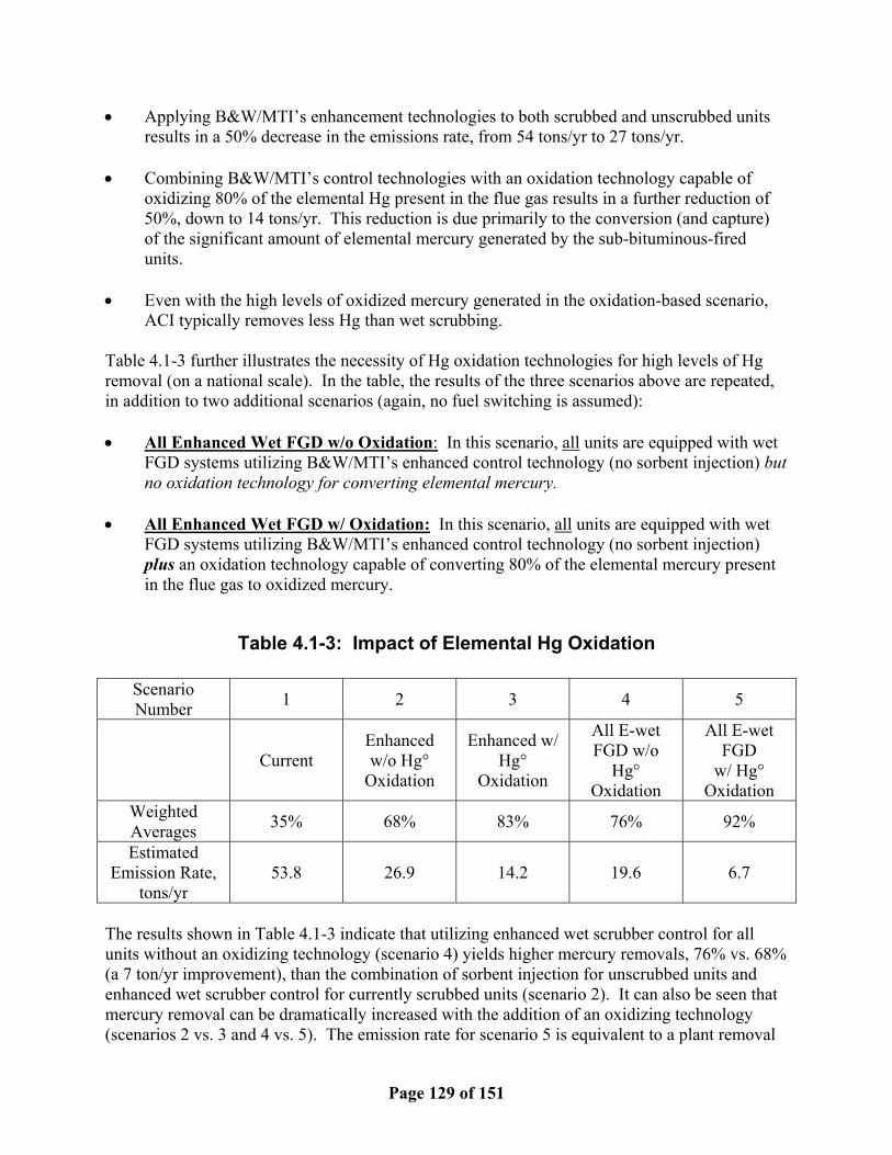
Page 129 of 151

• Applying B&W/MTI’s enhancement technologies to both scrubbed and unscrubbed units results in a 50% decrease in the emissions rate, from 54 tons/yr to 27 tons/yr.

• Combining B&W/MTI’s control technologies with an oxidation technology capable of

oxidizing 80% of the elemental Hg present in the flue gas results in a further reduction of 50%, down to 14 tons/yr. This reduction is due primarily to the conversion (and capture) of the significant amount of elemental mercury generated by the sub-bituminous-fired units.

• Even with the high levels of oxidized mercury generated in the oxidation-based scenario,

ACI typically removes less Hg than wet scrubbing. Table 4.1-3 further illustrates the necessity of Hg oxidation technologies for high levels of Hg removal (on a national scale). In the table, the results of the three scenarios above are repeated, in addition to two additional scenarios (again, no fuel switching is assumed): • All Enhanced Wet FGD w/o Oxidation: In this scenario, all units are equipped with wet

FGD systems utilizing B&W/MTI’s enhanced control technology (no sorbent injection) but no oxidation technology for converting elemental mercury.

• All Enhanced Wet FGD w/ Oxidation: In this scenario, all units are equipped with wet

FGD systems utilizing B&W/MTI’s enhanced control technology (no sorbent injection) plus an oxidation technology capable of converting 80% of the elemental mercury present in the flue gas to oxidized mercury.

Table 4.1-3: Impact of Elemental Hg Oxidation

Scenario Number 1 2 3 4 5

Current Enhanced w/o Hg°

Oxidation

Enhanced w/ Hg°

Oxidation

All E-wet FGD w/o

Hg° Oxidation

All E-wet FGD

w/ Hg° Oxidation

Weighted Averages 35% 68% 83% 76% 92%

Estimated Emission Rate,

tons/yr 53.8 26.9 14.2 19.6 6.7

The results shown in Table 4.1-3 indicate that utilizing enhanced wet scrubber control for all units without an oxidizing technology (scenario 4) yields higher mercury removals, 76% vs. 68% (a 7 ton/yr improvement), than the combination of sorbent injection for unscrubbed units and enhanced wet scrubber control for currently scrubbed units (scenario 2). It can also be seen that mercury removal can be dramatically increased with the addition of an oxidizing technology (scenarios 2 vs. 3 and 4 vs. 5). The emission rate for scenario 5 is equivalent to a plant removal

Page 130 of 151

rate (from as-fired coal to stack) of 92%, compared to a plant removal rate of 76% in the absence of an oxidation technology. Comparison with Competing Technologies To date, the most extensive mercury control research has been related to mercury capture via sorbent injection (either alkali-based or carbon-based). Most of the pilot- and demonstration-scale test programs have focused on the use of activated carbon injection (ACI) as the technology of choice for mercury control. This section compares the latest published mercury removal/cost information3,4,5 for ACI with B&W/MTI’s enhanced wet FGD-based process for a variety of scenarios. For the purposes of this discussion, the B&W/MTI process will be referred to as “E-Hg”. For all scenarios, particulate control is performed by an existing ESP. For each scenario, annual levelized costs (ALC) were calculated based on published removal/cost data for ACI and cost estimate modeling for E-Hg. For a more detailed discussion of how ALC values were determined, please see Section 4.5 – Process Economics. The following operational assumptions were made when performing the cost calculations: Size of Plant: 500 MW Capacity Factor: 65% Coal S: 3%, 1%, 0.3% Coal Hg: 0.23 ppm Cost of carbon: $0.425/lb Carbon feedrate: 5000:1, 9000:1, 15,000:1 lb AC/lb Hg Target Hg Removal: 80% Base Wet FGD Hg Removal: 70% Scenario 1: Existing Wet FGD + E-Hg vs. ACI Intended to represent the most likely initial target base for E-Hg, the model plant is firing a 3% sulfur coal and is equipped with a wet FGD system. Table 4.1-4 summarizes the results of the analysis and provides the estimated capital, operating and maintenance (O&M) costs both for applying B&W/MTI’s enhancement process to an existing wet FGD system, and for installing a new wet FGD system with the enhancement process. Reagent cost is the majority of the O&M costs. The table also includes what might be considered an equivalent evaluation using ACI technology solely for mercury capture at the 60 and 70 percent removal levels. Direct comparison of enhancement in an FGD system with ACI technology is difficult to establish given the fact that potential applications for each do not lend themselves to a direct comparison. Nevertheless, the incremental cost difference between the 60 and 70 percent removals with ACI may establish a better way to evaluate the relative cost benefit associated with improving mercury capture with the additive enhancement in a wet FGD system. Although it is highly unlikely that ACI would be used in a situation where the existing wet FGD system is already providing 70 percent removal, the 0.18 mil/kWh annual levelized cost of improving this to 80 percent with the additive technology is substantially below the 0.80 mil/kWh cost differential between achieving 60 and 70 percent removal with ACI. This is thought to illustrate the fact that enhanced mercury capture on its own represents minimal additional expense for scrubber-

Page 131 of 151

equipped utilities interest in reducing their mercury emissions and assuring that the mercury captured will be retained within the system rather than being re-emitted in the elemental form. While the values presented for ACI control are based on B&W/MTI’s own analysis of the cost of providing and operating an injection system, there are both positive and negative differences between the relative costs of capital and operating costs when compared to some of those reported by others. Because these differences are still being reconciled, no breakdown is provided on the capital and operating costs at this time. There is general agreement, however, between the costs developed here and the $2 – 5 million/yr range of overall annual levelized costs being reported by those working more directly on ACI control technologies.3,4,5

Table 4.1-4: Costs of Mercury Removal Processes

ENHANCED MERCURY CAPTURE IN A WET FGD

SYSTEM

Existing 500 MW Installation

New 500 MW Installation

Total Capital Requirement, $ 3,000,000 63,000,000

Total System O&M Costs, $/yr 125,000 3,200,000

Annual Levelized Cost, $/yr 500,000 12,000,000

Annual Levelized Cost, mil/kWh 0.18 4.23

MERCURY CAPTURE WITH

ACI TECHNOLOGY @ 60% Removal @ 70% Removal

Annual Levelized Cost, $/yr 2,400,000 4,700,000

Annual Levelized Cost, mil/kWh 0.85 1.65 The application of the B&W/MTI enhanced mercury capture process with a wet FGD system has the additional benefit of having virtually no impact on scrubber operation and gypsum quality. Moreover, it does not adversely affect the acceptability of fly ash for disposal/sale, a potential drawback ACI may have if it is not practical or economically attractive to separate by-product fly ash from the spent activated carbon. This aspect came to light in the demonstration of ACI at Wisconsin Electric’s Pleasant Prairie Power Plant where the carbon appeared to negate its use as a cement admixture. The economic impact in this case was estimated to be $12 to $15 million/yr due to lost fly ash sale revenue and increased landfill disposal costs.4

Page 132 of 151

Scenario 2: New Wet FGD + E-Hg vs. ACI + Spray Dryer Absorber (SDA) As further reductions in U.S. SO2 emissions become more likely to be enacted (see ‘Market Issues’ below), the installation of additional FGD capacity becomes more likely. In effect, the ‘threshold’ coal sulfur level, above which some type of FGD system would be required, would continue to decrease. As a result, new FGD systems would, in more and more cases, become financially attractive as the amount of ultra-low-sulfur coal would continue to decrease (and demand increase). In some instances, especially for units already firing lower sulfur coals, spray dryer absorbers (SDA) tend to be favored over wet FGD systems. If mercury control legislation is enacted in conjunction with more stringent SO2 emissions requirements, however, the choice of equipment becomes more intriguing. This scenario represents a potentially significant portion of the current U.S. generating market. For example, focusing solely on unscrubbed, ESP-equipped units east of the Mississippi firing bituminous coals encompasses 109,000 MW, one-third of the current generating capacity in the US. In this scenario, a low-sulfur coal (1%) is being fired in the 500 MW model plant. For the ACI + SDA options, it has been assumed that the addition of the SDA system will result in Hg removal performance comparable to wet FGD. In Table 4.1-5, the ALC (expressed in mil/kWh and $/yr) are shown for this comparison.

Table 4.1-5: Comparison of Wet FGD + E-Hg vs. ACI + SDA

ALC Wet FGD @ 70% Wet FGD + E-Hg @ 80%

ACI + SDA @ 70%

ACI + SDA @ 80%

mil/kWh 4.05 4.23 4.11 4.59 $/yr, 000’s 11,559 12,063 11,720 13,090

mil/kWh ∆, 70% to 80% 0.18 -- 0.48 $/yr, 000’s ∆, 70% to 80% 504 -- 1,370

The results shown in Table 4.1-5 illustrate two interesting observations. First and foremost, the addition of a wet FGD system (with or without E-Hg) for combined SO2 and Hg control is economically competitive with similarly performing ACI + SDA systems. Factoring in potential operational cost increases such as the ash disposal concerns mentioned in Scenario 1, and the application of a wet FGD-based system becomes even more attractive. Secondly, increasing the Hg removal performance for the wet FGD-based system through the addition of E-Hg is significantly less expensive than increasing the carbon feed rate to achieve the same performance for the ACI + SDA system. Scenario 3: New Wet FGD + E-Hg vs. ACI In some instances (ultra low-sulfur coal, SO2 credit surplus), more stringent SO2 emissions regulations will not require utilities to install new FGD control equipment. Any new equipment would be installed primarily for Hg control. For this scenario a very low-sulfur coal (0.3%) is being fired in the 500 MW model plant. Because a large portion of these low-sulfur coals are of the Western sub-bituminous variety, a much larger percentage of the mercury present in the flue

Page 133 of 151

gas is in the elemental form, which is not readily removed by wet FGD systems. Removal performance for the wet FGD estimates have been lowered to reflect an assumed 50:50 split between oxidized and elemental mercury (this does not affect wet FGD costs, only the corresponding ACI system). Similar to Scenario 2, this type of plant (low-sulfur, sub-bituminous coal, non-scrubbed, ESP-equipped) represents a potentially significant portion of the U.S. generating market (86,000 MW). In Table 4.1-6, the ALC (expressed in mil/kWh and $/yr) are shown for this comparison, along with estimated values for SO2 credits from the installation of a new wet FGD system (based on $150/ton SO2).

Table 4.1-6: Comparison of Wet FGD + E-Hg vs. ACI

ALC Wet FGD @ 50%

Wet FGD + E-Hg @ 60% ACI @ 60%

mil/kWh 4.05 4.23 0.85 $/yr, 000’s 11,559 12,063 2,426

SO2 credit, $/yr 000’s 946 946 --

Given the significant capital requirement for wet FGD systems, it is not surprising that installing these systems solely for Hg control will not generally be economically viable. Only in those situations where an increase in carbon content in the fly ash would result in significant operating cost increases (higher disposal costs, loss of by-product sale, etc.) would it potentially become attractive to install wet FGD for Hg control. 4.2 BY-PRODUCT MARKET An important consideration for a successful mercury control technology is that of waste generation. Additionally, for mercury control processes which are “add-ons” to existing pollution control processes (i.e. wet FGD), minimizing the effect on usable by-products is highly desirable. The reagent used during this program is fed to the wet scrubber in very small amounts. The feed rates were approximately 1 gallon/hour at Endicott (55 MWe) and 5.4 gallon/hour per absorber at Zimmer (5 operating absorbers, 1300 MWe) and does not accumulate in the slurry. Excess reagent reacts with other constituents in the slurry or is volatilized and exits with the flue gas. This reagent also does not affect slurry quality or the SO2 removal performance of the scrubber system. The only by-product potentially formed by this process would be generated from the additional capture of mercury (above baseline removal performance). During this program, various process samples were analyzed in an attempt to identify mercury compounds formed in the scrubber and to determine their stability. The results of this work indicated that 1) all mercury compounds formed through this process are essentially insoluble and are thermally stable over the temperature range of typical wallboard manufacturing processes, and 2) the mercury captured in the wet scrubber is present as a fine particulate; the use of blowdown and other purge streams containing fine particulate can effectively maintain low Hg concentrations in the scrubber

Page 134 of 151

gypsum by-product. In addition, even with the increased mercury removal performance achieved by this process, the disposal status of the gypsum generated in the scrubber is not adversely affected. These points are discussed in more detail in Section 3.5. 4.3 MARKETPLACE ACCEPTANCE Potential barriers to commercial application of B&W/MTI’s enhanced mercury control technology may be classified as technical, market, or regulatory. Although several potential obstacles will be discussed, no one single concern is expected to prevent commercial application of the technology. Conversely, because mercury emissions from coal-fired boilers are currently not regulated (with the exception of a couple of pending state requirements), utilities are not likely to install any control equipment until some indication of control requirements and corresponding timeframe for compliance is available. Technical Issues The control technology demonstrated during this program represents a low-cost, non-intrusive method of enhancing mercury removal performance for wet FGD-equipped utility power plants. Because it relies on the presence of a wet FGD system, however, initial applications of the technology will be limited to 1) those units currently equipped with a wet FGD system, and 2) new wet FGD construction. Additionally, mercury removal performance results from this program have identified a number of potential technical limitations and uncertainties which will need to be addressed prior to successful market application. These include: • Impact of Hg speciation – Mercury in the oxidized form is readily captured by wet FGD

systems; elemental mercury is essentially unaffected. As a result, the ratio of the oxidized:elemental mercury entering a utility wet FGD system will have a direct impact on the upper removal performance limit of the control technology. For bituminous-fired units with unusually low concentrations of oxidized mercury, or for units firing sub-bituminous coals, which typically generate high percentages of elemental mercury, additional processes or technologies which improve mercury oxidation may be required should mercury control regulations stipulate high removal levels.

• Impact of Wet FGD chemistry – During this program, two different scrubber chemistries

were encountered: the Endicott wet FGD system is limestone-based with in situ forced oxidation (LSFO); the Zimmer wet FGD system is Thiosorbic® Lime-based with natural oxidation in the scrubber and ex situ forced oxidation system for gypsum production. As mentioned in Section 3, this difference was not expected to have an impact on mercury removal performance; the test results indicated otherwise. Because all of the development work on this technology (and 1 of the 2 demonstration tests) was performed with limestone-based, in situ forced oxidation systems, it is uncertain how well it will perform in scrubber systems based on different chemical processes. Currently, one-third of the wet scrubber-equipped U.S. generating capacity (approx. 27,000 MW) is utilizing non-LSFO chemistry scrubber systems (although LSFO FGD and dry FGD are expected to become the technologies of choice and increase their market share).

Page 135 of 151

• Concentration of Captured Mercury – As shown in Section 3.5, the mercury captured in an enhanced wet FGD system tends to be present as a fine particulate. As such, in unit operations such as hydroclone separation, the mercury will preferentially report to the dilute phase. This behavior serves to not only minimize the amount of mercury reporting to the gypsum, but offers the potential for reduced waste treatment costs by concentrating the captured mercury in a single stream (e.g., blowdown or purge stream).

Market Issues The widespread acceptance and application of mercury control technologies (in general) will quite likely be highly dependent upon other pollutant emission requirements. Several recent trends indicate an increased potential for long-term application of B&W/MTI’s enhancement process: • Increased trend toward scrubbing vs. coal switching – A resurgence of demand for FGD

systems is expected not only because emissions regulations are becoming more stringent but also because banked SO2 allowances resulting from the 1990 Clean Air Act are rapidly being depleted. The requirement of FGD, especially in the eastern U.S., will cause a re-evaluation of fuel type versus cost and should result in some fuel switching back to higher sulfur, lower cost eastern fuels for units that previously switched to low-sulfur fuels to avoid scrubbing. The higher sulfur fuels coupled with increased SO3 emissions aggravated by SCR (selective catalytic reduction) installations will pose the problem of visible sulfuric acid plumes.

• Interaction with other pollution control processes – The release of the NOx SIP call

requires the reduction of NOx emissions, primarily via SCR, for the 24 states east of the Mississippi River. Coincidentally, this same region is where most of the high sulfur coal is fired in the U.S. Compliance with the SIP call is well underway; numerous new SCR installations are online or in the planning stages. Initial research into the effect of SCR catalysts on mercury speciation has shown that, in some instances, significant oxidation of elemental mercury is observed. Since SCRs are installed upstream of wet FGD systems, any increase in the percentage of oxidized mercury in the flue gas will improve the removal performance for the wet FGD system.

Regulatory Issues With the exception of Wisconsin (and more recently, North Carolina), mercury emission control requirements at the federal and state level have not yet been promulgated. Because of the demonstrated technology’s reliance on wet FGD systems, however, developments in SOx (and to a lesser extent, NOx) emission regulations could have an impact on the extent and timing of market application. Recent federal regulatory developments indicate that further reductions in NOx and SOx emissions are under increased scrutiny. The Jefford’s Bill, which calls for significant further reductions of SOx (72%), NOx (75%) and mercury (90%) emissions, was recently approved in committee hearings. Although it is questionable whether the Bill will pass in its current form, its

Page 136 of 151

successful committee discussion indicates that utility-generated pollution levels are foremost in Federal discussions. It is currently anticipated that some form of this Bill will supplant the New Source Review Requirements of the CAAA of 1990.

From a state regulatory viewpoint, many states, such as Massachusetts, New Hampshire, Connecticut and more recently North Carolina are seeking to clean up coal-fired units by imposing emissions regulations that are often more stringent than federal regulations rather than seeking ways to replace coal. In some instances, these state requirements are incorporating Hg emission control requirements, in addition to NOx and SOx emission reductions.

4.4 INCREASED USE OF OHIO COAL According to utility plant data available from the US EPA, approximately 7,600 MW (31 units) of installed generating capacity is currently firing Ohio coal. Of that amount, approximately 4,300 MW (8 units) is scrubbed. Of the 7,600 MW burning Ohio coal, 5,300 MW (3,600 MW scrubbed) is located in the state of Ohio. Total installed generating capacity in the state of Ohio is 23,300 MW. Table 4.4-1 presents a summary of this data, along with related percentage calculations regarding the current use of Ohio coal.

Table 4.4-1: Current Status of Ohio Coal Use and Ohio Generating Capacity

Total Wet FGD Percentage Ohio Generating Capacity, MW 23,300 5,000 21%

- firing Ohio coal 5,300 3,600 68% Percent of Ohio Total 23% 72%

US Generating Capacity, MW 307,000 80,600 26% - firing Ohio coal 7,600 4,300 57%

Percent of US Total 2.5% 5.3%

Based on the numbers provided in Table 4.6, the most likely source of increased Ohio coal usage is within the state of Ohio. Only 23% of the generating capacity is fired by Ohio coal, most likely due to emission restrictions. Furthermore, some of the scrubbed generating capacity is currently fired by non-Ohio coal (1,400 MW). 4.5 PROCESS ECONOMICS In section 4.1, annual levelized costs (ALC) were estimated for several scenarios. This section provides additional information regarding the calculation of the values presented in each scenario. Each ALC was calculated based on a Total Capital requirement, distributed over a 20 year life, plus yearly operating and maintenance costs. EPRI’s (Electric Power Research Institute) TAGTM Technical Assessment Guide (EPRI Report P-6587-L) was used as the basis for the calculations. The starting point for the Total Capital requirement was the installed equipment cost – all other capital/investment costs were determined by applying factors to the installed equipment cost. Included as other capital/investment costs were engineering, general facilities,

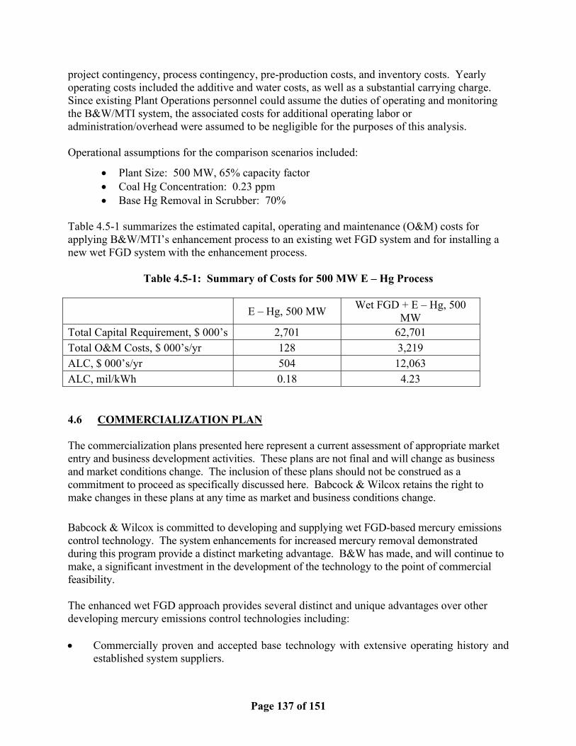
Page 137 of 151

project contingency, process contingency, pre-production costs, and inventory costs. Yearly operating costs included the additive and water costs, as well as a substantial carrying charge. Since existing Plant Operations personnel could assume the duties of operating and monitoring the B&W/MTI system, the associated costs for additional operating labor or administration/overhead were assumed to be negligible for the purposes of this analysis. Operational assumptions for the comparison scenarios included:

• Plant Size: 500 MW, 65% capacity factor • Coal Hg Concentration: 0.23 ppm • Base Hg Removal in Scrubber: 70%

Table 4.5-1 summarizes the estimated capital, operating and maintenance (O&M) costs for applying B&W/MTI’s enhancement process to an existing wet FGD system and for installing a new wet FGD system with the enhancement process.

Table 4.5-1: Summary of Costs for 500 MW E – Hg Process

E – Hg, 500 MW Wet FGD + E – Hg, 500 MW

Total Capital Requirement, $ 000’s 2,701 62,701 Total O&M Costs, $ 000’s/yr 128 3,219 ALC, $ 000’s/yr 504 12,063 ALC, mil/kWh 0.18 4.23 4.6 COMMERCIALIZATION PLAN The commercialization plans presented here represent a current assessment of appropriate market entry and business development activities. These plans are not final and will change as business and market conditions change. The inclusion of these plans should not be construed as a commitment to proceed as specifically discussed here. Babcock & Wilcox retains the right to make changes in these plans at any time as market and business conditions change. Babcock & Wilcox is committed to developing and supplying wet FGD-based mercury emissions control technology. The system enhancements for increased mercury removal demonstrated during this program provide a distinct marketing advantage. B&W has made, and will continue to make, a significant investment in the development of the technology to the point of commercial feasibility. The enhanced wet FGD approach provides several distinct and unique advantages over other developing mercury emissions control technologies including: • Commercially proven and accepted base technology with extensive operating history and

established system suppliers.

Page 138 of 151

• Established by-product market for FGD gypsum. • Limited additional hardware • Simple operation • Lower operating costs than alternatives in many situations • Readily available reagent with established suppliers with existing production capacity. All of the above factors make B&W/MTI’s process an attractive option for enhancing mercury control performance for wet FGD systems. Until regulations governing mercury emissions levels are issued, however, the extent to which this, or any, control process will be implemented will be minimal. As mentioned above, several emerging trends in the environmental emissions control market, however, may have a favorable impact on commercialization of B&W/MTI’s process. Some of these current favorable trends include: • Multi-pollutant emissions regulation potential • States moving forward to address mercury control in phased approach: allowing FGD only

to meet initial near-term requirements; B&W’s enhancements would be used to increase removal as needed to meet later requirements – 10 to 15 years out.

• NSR pushing potential wet FGD market • Increasing preference to scrub over fuel switching

Page 139 of 151

5.0 REFERENCES 1. McDonald, D. K., Amrhein, G. T., Kudlac, G. A., and Yurchison, D. A., Mercury Control

for Coal-Fired Utilities, Final Report, March 2002. This project was jointly funded by the Ohio Coal Development Office within the Ohio Department of Development and Babcock & Wilcox.

2. The Gypsum Industry and Flue Gas Desulfurization (FGD) Gypsum Utilization: A Utility Guide, EPRI Technical Report TR-103652, February 1994

3. “Full-Scale Test of Mercury Control with Sorbent Injection and an ESP at Wisconsin

Electric’s Pleasant Prairie Power Plant,” T. Starns, et al., Paper No. 43249, presented at the Air & Waste Management Association’s 95th Annual Meeting & Exhibition, Baltimore, MD, June 2002

4. “Operational and Maintenance Impacts of Hg Control,” T. Coughlin, Paper presented at the

Scientech Mercury Emissions Workshop, Clearwater Beach, FL, January 2002 5. “Predicted Costs of Mercury Control at Electric Utilities,” F. B. Meserole, Paper presented

at the Scientech Mercury Emissions Workshop, Clearwater Beach, FL, January 2002 6. Felsvang, K.S., et al., “Method of Improving the Hg-Removing Capability of a FLue Gas

Cleaning Device”, U.S. Patent 5,435,980, July 25, 1995. 7. Farzan, H., et al, “Cost-Effective Control of NOx with Integrated Ultra Low-NOx Burners

and SNCR”, U.S.DOE Contract DE-FC26-99FT40717, December, 2002. 8. Mercury Control for Coal-Fired Boilers, Technical Report for the Period Dec-Mar 2001,

Ohio Coal Development Office Grant Agreement CDO/D-98-7, April 19, 2001

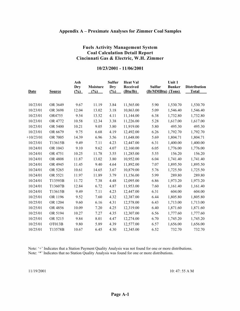
Page A-1

Appendix A – Proximate Analyses for Zimmer Coal Samples

Fuels Activity Management System Coal Calculation Detail Report

Cincinnati Gas & Electric, W.H. Zimmer

10/23/2001 - 11/06/2001 Ash Sulfur Heat Val Unit 1 Dry Moisture Dry Received Sulfur Bunker Distribution Date Source (%) (%) (%) (Btu/lb) (lb/MMBtu) (Tons) Total 10/23/01 OR 3649 9.67 11.19 3.84 11,565.00 5.90 1,530.70 1,530.70 10/23/01 OR 3698 12.04 13.02 3.18 10,863.00 5.09 1,546.40 1,546.40 10/23/01 OR4755 9.54 13.52 4.11 11,144.00 6.38 1,732.80 1,732.80 10/23/01 OR 4772 10.58 12.34 3.38 11,226.00 5.28 1,617.00 1,617.00 10/23/01 OR 5400 10.21 9.05 3.80 11,919.00 5.80 495.30 495.30 10/23/01 OR 6679 9.75 6.68 4.19 12,492.00 6.26 1,792.70 1,792.70

+10/23/01 OR 7005 14.39 6.96 3.56 11,648.00 5.69 1,804.71 1,804.71 10/23/01 T13615B 9.49 7.11 4.23 12,447.00 6.31 1,400.00 1,400.00 10/24/01 OR 1043 9.10 9.62 4.07 12,160.00 6.05 1,776.00 1,776.00 10/24/01 OR 4751 10.25 11.78 3.55 11,285.00 5.55 156.20 156.20 10/24/01 OR 4808 11.87 13.02 3.80 10,952.00 6.04 1,741.40 1,741.40 10/24/01 OR 4945 11.45 9.40 4.64 11,892.00 7.07 1,895.50 1,895.50 10/24/01 OR 5265 10.61 14.65 3.67 10,879.00 5.76 1,725.50 1,725.50 10/24/01 OR 5521 11.97 11.89 3.79 11,156.00 5.99 289.80 289.80 10/24/01 T13593B 11.72 7.38 4.48 12,095.00 6.86 1,973.20 1,973.20 10/24/01 T13607B 12.84 6.72 4.87 11,953.00 7.60 1,161.40 1,161.40 10/24/01 T13615B 9.49 7.11 4.23 12,447.00 6.31 604.00 604.00 10/25/01 OR 1196 9.52 7.60 4.32 12,387.00 6.44 1,805.80 1,805.80 10/25/01 OR 1204 9.60 6.16 4.31 12,578.00 6.43 1,713.00 1,713.00 10/25/01 OR 4856 10.09 7.20 4.25 12,319.00 6.40 1,871.60 1,871.60 10/25/01 OR 5194 10.27 7.27 4.35 12,307.00 6.56 1,777.60 1,777.60 10/25/01 OR 5215 9.84 8.01 4.47 12,274.00 6.70 1,745.20 1,745.20 10/25/01 OT013B 9.80 5.89 4.39 12,577.00 6.57 1,656.00 1,656.00 10/25/01 T13578B 10.67 6.45 4.30 12,345.00 6.52 732.70 732.70 Note: ‘+’ Indicates that a Station Payment Quality Analysis was not found for one or more distributions. Note: ‘*’ Indicates that no Station Quality Analysis was found for one or more distributions. 11/19/2001 10: 47: 55 A M

Page A-2



10/23/2001 - 11/06/2001 Ash Sulfur Heat Val Unit 1 Dry Moisture Dry Received Sulfur Bunker Distribution Date Source (%) (%) (%) (Btu/lb) (lb/MMBtu) (Tons) Total 10/25/01 T13607B 12.84 6.72 4.87 11,953.00 7.60 816.50 816.50 10/26/01 OR3762 9.50 6.82 4.13 12,483.00 6.17 1,707.00 1,707.00 10/26/01 OR 4840 11.69 7.61 3.07 12,208.00 4.65 957.20 957.20 10/26/01 OR5210 9.28 6.74 4.23 12,462.00 6.33 1,125.00 1,125.00 10/26/01 OR 5349 9.06 6.24 4.17 12,634.00 6.19 1,840.80 1,840.80 10/26/01 OR 5389 9.57 7.16 4.00 12,456.00 5.96 1,856.70 1,856.70 10/26/01 OR 5404 9.98 6.63 4.44 12,405.00 6.68 1,200.30 1,200.30 10/26/01 OR 5515 9.30 7.75 4.42 12,223.00 6.67 1,822.00 1,822.00 10/26/01 OR 5519 10.68 12.47 3.39 11,143.00 5.33 1,697.10 1,697.10 10/27/01 OR 3618 12.42 12.68 3.70 10,776.00 6.00 173.80 173.80 10/27/01 OR 3863 9.41 6.22 4.20 12,578.00 6.26 543.20 543.20 10/27/01 OR 5210 9.28 6.74 4.23 12,462.00 6.33 654.70 654.70 10/27/01 OR 5430 9.14 7.32 4.50 12,426.00 6.71 1,885.90 1,885.90 10/27/01 OR 5548 11.12 9.78 4.36 11,554.00 6.81 1,713.20 1,713.20 10/27/01 OR 9040 9.17 6.79 4.15 12,546.00 6.17 1,611.40 1,611.40

+10/27/01 OT003B 12.78 6.07 3.78 11,958.00 5.94 1,928.00 1,928.00 10/27/01 T13635B 9.39 7.92 3.93 12,340.00 5.87 1,877.50 1,877.50 10/28/01 OR 1032 9.75 6.98 4.15 12,407.00 6.22 1,743.80 1,743.80 10/28/01 OR 1222 10.24 9.38 3.46 11,705.00 5.36 1,560.90 1,560.90 10/28/01 OR 4764 9.87 5.97 4.33 12,536.00 6.50 1,828.90 1,828.90 10/28/01 OR 5143 8.92 6.75 4.17 12,606.00 6.17 295.70 295.70 10/28/01 OR 5198 15.68 6.94 3.27 11,449.00 5.32 1,512.80 1,512.80 10/28/01 OR 5428 10.00 7.43 2.99 0.00 0.00 1,675.50 1,675.50 10/28/01 T13617B 9.38 6.34 4.31 12,526.00 6.45 1,954.20 1,954.20 Note: ‘+’ Indicates that a Station Payment Quality Analysis was not found for one or more distributions. Note: ‘*’ Indicates that no Station Quality Analysis was found for one or more distributions. 11/19/2001 10: 47: 55 A M

Page A-3



10/23/2001 - 11/06/2001 Ash Sulfur Heat Val Unit 1 Dry Moisture Dry Received Sulfur Bunker Distribution Date Source (%) (%) (%) (Btu/lb) (lb/MMBtu) (Tons) Total 10/29/01 OR 3748 11.50 6.28 3.82 12,189.00 5.87 232.00 232.00 10/29/01 OR 3752 10.35 7.79 2.95 12,288.00 4.43 1,672.50 1,672.50

+10/29/01 OR 3755 14.92 6.58 3.03 11,365.00 4.98 1,485.70 1,485.70 10/29/01 OR 4924 10.17 7.22 3.13 12,490.00 4.65 1,718.80 1,718.80 10/29/01 OR 5060 9.46 6.32 4.05 12,595.00 6.02 1,593.70 1,593.70

+10/29/01 OR 5442 14.91 6.03 3.75 11,683.00 6.03 1,927.00 1,927.00 +10/29/01 OR 5502 6.60 5.50 2.46 13,445.00 3.46 310.70 310.70 10/29/01 OR 5512 12.59 6.75 4.23 11,984.00 6.58 1,858.30 1,858.30 10/29/01 T13509B 10.04 7.21 4.19 0.00 0.00 1,932.00 1,932.00

+10/30/01 OR 1176 12.99 5.57 3.74 12,065.00 5.85 83.87 83.87 10/30/01 OR 4875 12.15 7.36 4.55 11,911.00 7.08 1,375.10 1,375.10 10/30/01 OR 5117 11.87 9.38 3.74 11,465.00 5.91 492.80 492.80 10/30/01 OR 5207 13.76 11.05 3.57 11,228.00 5.66 1,264.20 1,264.20 10/30/01 OR 5263 11.08 7.58 4.03 12,061.00 6.18 1,769.90 1,769.90 10/30/01 OR 5312 10.48 8.42 3.94 12,048.00 5.99 1,869.40 1,869.40 10/30/01 OR 5375 12.06 7.88 4.23 11,887.00 6.56 1,794.80 1,794.80 10/30/01 OR 5498 11.63 9.96 3.74 11,361.00 5.93 1,549.00 1,549.00 10/30/01 OR 9006 9.47 8.16 4.04 12,300.00 6.03 1,177.40 1,177.40 10/31/01 OR 3772 8.77 7.21 3.97 12,534.00 5.88 1,625.70 1,625.70 10/31/01 OR 9006 9.47 8.16 4.04 12,300.00 6.03 677.80 677.80 11/01/01 High Sulfur Pile 10.32 8.42 3.39 11,985.00 5.18 8,776.80 8,776.80

+11/01/01 OR 5001 14.26 6.49 4.19 11,712.00 6.69 242.10 242.10 11/01/01 OR 5475 9.50 6.05 3.99 12,627.00 5.94 1,849.00 1,849.00 11/01/01 T13603B 9.94 7.34 4.14 12,309.00 6.23 1,758.30 1,758.30 Note: ‘+’ Indicates that a Station Payment Quality Analysis was not found for one or more distributions. Note: ‘*’ Indicates that no Station Quality Analysis was found for one or more distributions. 11/19/2001 10: 47: 55 A M

Page A-4



10/23/2001 - 11/06/2001 Ash Sulfur Heat Val Unit 1 Dry Moisture Dry Received Sulfur Bunker Distribution Date Source (%) (%) (%) (Btu/lb) (lb/MMBtu) (Tons) Total 11/02/01 High Sulfur Pile 10.32 8.42 3.32 11,985.00 5.07 844.00 844.00 11/02/01 OR 5129 10.09 10.10 3.66 11,608.00 5.67 1,559.30 1,559.30

+11/02/01 OR 5388 14.37 8.38 1.49 11,388.00 2.40 1,872.90 1,872.90 11/02/01 OR 5487 9.98 7.01 4.17 12,427.00 6.24 1,834.70 1,834.70

+11/02/01 T13519B 14.54 6.38 3.29 11,739.00 5.25 2,014.33 2,014.33 +11/02/01 T13598B 17.44 6.60 1.13 11,495.00 1.84 1,910.57 1,910.57 +11/02/01 T13607B 17.06 8.36 1.17 11,111.00 1.93 2,029.63 2,029.63 +11/03/01 OR4755 19.90 5.99 1.44 11,059.00 2.45 1,692.10 1,692.10 +11/03/01 OR 4846 16.97 8.83 1.06 10,925.00 1.77 1,821.28 1,821.28 +11/03/01 OR4857 15.47 8.35 4.11 11,382.00 6.62 195.42 195.42 +11/03/01 OR 5165 13.88 7.59 3.91 11,654.00 6.20 62.92 62.92 +11/03/01 OR 5521 9.94 5.67 4.22 12,567.00 6.34 1,825.80 1,825.80 11/03/01 OR 7043 9.60 6.72 3.99 12,416.00 6.00 1,850.40 1,850.40

+11/04/01 OR 1019 14.78 8.11 3.89 11,447.00 6.25 1,541.77 1,541.77 +11/04/01 OR 1196 18.12 7.74 1.04 11,082.00 1.73 1,723.93 1,723.93 11/04/01 OR 4799 11.86 5.76 3.94 12,268.00 6.05 1,520.00 1,520.00 11/04/01 OR 5135 21.07 5.87 1.35 11,125.00 2.28 1,713.50 1,713.50 11/04/01 OR5359 11.38 6.21 4.11 12,463.00 6.19 1,867.00 1,867.00 11/04/01 OR5467 10.72 5.85 4.06 12,441.00 6.14 1,850.90 1,850.90 11/05/01 OR4799 11.86 5.76 3.94 12,268.00 6.05 70.30 70.30 11/05/01 OR4807 10.47 9.81 3.80 11,637.00 5.89 1,733.60 1,733.60 11/05/01 OR4819 11.06 5.96 4.10 12,332.00 6.25 1,863.00 1,863.00 11/05/01 OR4890 12.47 5.82 4.17 12,144.00 6.47 1,808.60 1,808.60 11/05/01 OR5137 13.78 5.62 3.67 11,929.00 5.81 1,666.00 1,666.00 Note: ‘+’ Indicates that a Station Payment Quality Analysis was not found for one or more distributions. Note: ‘*’ Indicates that no Station Quality Analysis was found for one or more distributions. 11/19/2001 10: 47: 55 A M

Page A-5



10/23/2001 - 11/06/2001 Dry Moisture Dry Received Sulfur Bunker Distribution Date Source (%) (%) (%) (Btu/lb) (lb/MMBtu) (Tons) Total 11/05/01 OR 5410 11.85 8.87 4.25 11,549.00 6.71 286.80 286.80 11/05/01 OR 9042 14.71 8.55 4.73 11,195.00 7.73 1,625.40 1,625.40 11/05/01 T13600B 13.11 6.21 4.69 11,932.00 7.37 690.30 690.30 11/06/01 OR 4802 9.71 6.66 4.10 12,489.00 6.13 1,848.00 1,848.00 11/06/01 OR 4813 10.52 6.16 4.31 12,421.00 6.51 1,893.80 1,893.80 11/06/01 OR 4821 11.10 5.75 4.45 12,412.00 6.76 1,858.30 1,858.30 11/06/01 OR 5321 9.50 5.84 3.99 12,626.00 5.95 1,239.70 1,239.70 11/06/01 OR 6685 10.13 9.19 3.20 11,964.00 4.86 460.00 460.00 11/06/01 R 0204 10.05 6.09 4.17 12,489.00 6.27 1,821.30 1,821.30 11/06/01 T13575B 9.60 5.99 4.14 12,517.00 6.22 1,966.00 1,966.00 Note: ‘+’ Indicates that a Station Payment Quality Analysis was not found for one or more distributions. Note: ‘*’ Indicates that no Station Quality Analysis was found for one or more distributions. 11/19/2001 10: 47: 55 A M

Page B-1

Appendix B – Plant Data Acquisition System Data

Below are several tables showing the average values for all of the operating data acquired during the project for each test.

Ontario Hydro Plant CO2 In Plant CO2 Out Plant SO2 Plant SO2 In Plant SO2 OutPlant SO2

Removal Efficiency

Plant NOX Plant NOX Plant Flow Plant Flow Plant Flow Plant Heat Rate Plant Load Plant Opacity Plant Temp

Stack

Test ID % % lb/hr ppm (wet) ppm (wet) % lb/hr ppm (dry) kcfm scfh fps mmBTU/hr MW % oF

050801-1A1 9.96 12.01 0.300 1218 120 91.8 3.65 181 117 11925263 16.1 796 55.7 2.96 117050901-1B 9.72 12.11 0.320 1387 130 92.5 4.26 197 116 12360567 16.6 832 59.3 3.03 116050901-1C 9.48 11.91 0.363 1520 144 92.4 4.79 199 118 13059869 17.3 864 60.6 3.05 118050901-1D 9.41 11.90 0.344 1438 137 92.5 4.57 195 119 12980441 17.3 858 59.5 3.50 119051601-2A 9.30 11.70 0.440 1543 172 91.1 4.96 208 118 12817695 17.2 833 59.3 2.97 118051601-2B 8.90 11.36 0.492 1605 187 90.9 5.39 187 118 12321562 16.9 778 55.0 2.73 118051701-3A 9.34 11.81 0.497 1797 196 91.4 5.75 203 119 12414452 17.0 814 57.7 2.56 119051701-3B 9.73 11.95 0.443 1700 177 91.5 5.22 196 121 12800454 17.4 850 58.2 2.75 121051701-3C 10.02 12.09 0.405 1616 164 91.6 4.82 182 123 13237993 17.9 889 59.4 3.01 123051801-4A 9.47 11.79 0.453 1647 179 91.3 5.20 189 120 12197413 16.7 800 56.6 2.80 120051801-4B 9.45 11.78 0.479 1668 189 90.9 5.27 200 119 12363792 16.9 809 58.4 2.71 119051801-4C 9.76 11.85 0.464 1710 184 91.1 5.24 181 120 11616800 16.1 764 55.9 2.66 120061101-5A 9.25 11.91 0.994 2385 396 87.3 7.70 176 121 12074642 16.7 799 55.8 4.41 121061101-5B 9.29 11.84 0.506 2047 200 92.3 6.59 181 123 12296832 16.9 809 53.1 3.20 123061101-5C 9.34 11.93 0.587 1815 234 89.9 5.81 183 123 13055528 17.8 865 55.8 4.04 123061201-6A 9.80 11.92 0.431 1793 172 92.1 5.46 179 120 12034334 16.6 797 56.1 3.06 120061201-6B 10.02 12.00 0.386 1681 155 92.3 5.01 181 122 12373427 16.9 825 55.0 3.56 122061301-7A 9.87 12.12 0.388 1449 157 91.2 4.39 177 122 11953799 16.6 805 53.9 3.83 122061301-7B 9.70 11.92 0.493 1626 197 90.2 5.00 177 123 12584057 17.2 833 53.0 4.15 123061301-7C 9.63 11.88 0.374 1553 149 92.3 4.82 181 124 12554602 17.2 829 53.0 4.89 124061401-8A 9.80 12.03 0.385 1568 155 91.9 4.78 180 122 12026472 16.5 804 53.0 4.82 122061401-8B 9.97 12.05 0.357 1448 144 91.8 4.34 181 122 12336097 16.9 825 53.0 5.54 122061401-8C 10.01 12.08 0.406 1605 164 91.5 4.79 183 122 12349132 16.9 828 53.1 5.99 122062501-9A 10.11 13.01 0.468 1983 204 92.0 5.86 198 122 12792874 17.2 924 56.7 3.23 122062601-10A 9.82 12.70 0.609 2052 259 90.3 6.26 187 121 12585846 17.0 887 55.9 3.15 121062701-11A 12.58 11.35 0.308 1917 134 94.9 4.56 193 122 13196197 17.5 818 55.1 3.01 122062801-12A 11.91 10.91 0.564 1827 191 87.5 4.59 432 121 12330311 16.8 721 56.9 3.07 121062901-13A 11.82 10.38 0.420 1916 146 91.3 4.84 186 122 12897961 17.4 744 54.9 3.23 122063001-14A 11.71 10.05 0.368 1683 124 91.4 4.30 160 124 12565964 17.2 702 54.8 3.28 124070101-15A 10.43 8.95 0.315 1634 95 93.3 4.68 139 117 9535192 13.9 474 37.7 3.11 117070201-16A 11.33 10.39 0.337 1904 117 93.3 5.02 147 112 9594815 13.8 556 44.0 3.10 112

Plant Data

Table B1 – Endicott Operating Data

Page B-2

Ontario Hydro Plant CO 2 In Plant CO 2 Out Plant SO 2 Plant SO 2 In Plant SO 2 OutPlant SO 2RemovalEfficiency

Plant NO X Plant NO X Plant Flow Plant Flow Plant FlowPlant Heat

RatePlant Load Plant Opacity

Plant TempStack

Test ID % % lb/hr ppm (wet) ppm (wet) % lb/hr ppm (dry) kcfm scfh fps mmBTU/hr MW % oF

070601-17A 12.44 9.84 0.303 1711 100 92.6 4.11 136 118 9102964 13.5 498 46.9 3.13 118070701-18A 11.26 8.88 0.256 1489 76 93.5 3.95 171 117 8404419 12.8 415 36.8 3.29 117070801-19A 11.63 9.39 0.269 1552 84 93.3 3.99 194 122 9155271 13.8 478 43.8 3.18 122070901-20A 12.12 11.75 0.351 1945 138 92.7 4.80 183 122 10865267 15.4 709 57.2 3.02 122071001-21A 11.76 10.53 0.291 1690 102 93.2 4.30 198 122 10926233 15.5 639 55.8 2.97 122071101-22A 10.43 10.75 0.349 1820 126 93.3 5.22 191 118 11154079 15.5 667 57.8 3.45 118071201-23A 12.17 11.16 0.374 1935 140 92.1 4.75 160 118 11480691 15.8 711 57.1 2.74 118071201-23B 12.38 11.40 0.386 1980 147 91.9 4.78 164 119 10811263 15.2 684 57.2 2.67 119071201-23C 12.22 11.80 0.351 1839 139 92.2 4.50 171 120 10592030 15.0 694 56.2 2.87 120072401-24A 12.44 9.53 0.393 2033 125 92.0 4.88 180 124 11032786 15.7 584 56.6 3.11 124072401-24B 12.66 9.37 0.479 2175 150 90.7 5.13 184 125 11172364 15.9 582 56.3 3.21 125072401-24C 12.45 9.12 0.786 2272 240 85.6 5.45 177 126 11172695 15.9 566 54.7 3.12 126080701-25A 12.02 10.77 0.362 1745 130 91.6 4.34 169 122 9478722 14.0 567 48.4 3.23 122080701-25B 12.06 10.39 0.488 2095 170 90.6 5.19 168 124 9315407 13.9 537 46.3 3.24 124080701-25C 11.97 10.19 0.660 2311 225 88.6 5.77 159 125 9603581 14.3 543 45.1 3.30 125082101-26A 12.34 10.59 0.367 1801 130 91.6 4.36 136 119 10797994 15.2 636 53.9 3.86 119082101-26B 12.29 10.53 0.437 1984 154 90.9 4.83 147 120 10395665 14.8 608 55.6 3.54 120082101-26C 12.48 10.66 0.399 1857 143 91.0 4.45 147 120 10805861 15.2 640 57.7 3.66 120090501-27A 12.37 10.76 0.415 1924 149 91.1 4.65 162 119 11088446 15.4 663 55.9 14.66 119090501-27B 12.23 10.76 0.407 1911 146 91.3 4.67 170 120 10608506 15.0 634 55.6 8.03 120090501-27C 12.32 10.53 0.397 1845 140 91.1 4.47 177 120 11302041 15.6 661 57.1 10.23 120091801-28A 12.21 10.59 0.433 1949 153 90.9 4.77 154 119 11174951 15.6 657 57.0 2.59 119091801-28B 12.23 10.64 0.447 1982 159 90.8 4.84 171 119 11126660 15.6 658 56.9 3.13 119091801-28C 12.47 10.74 0.454 2046 163 90.7 4.90 165 120 11294249 15.8 674 57.1 3.30 120100201-29A 12.77 11.89 0.559 2157 233 88.4 5.05 194 121 11908949 16.4 788 59.3 3.28 121100201-29B 12.66 10.91 0.653 2091 238 86.8 4.94 172 121 11529287 16.0 699 59.2 3.34 121100201-29C 12.83 10.94 0.519 1975 190 88.7 4.60 168 122 11414970 15.9 694 58.9 5.57 122100301-30A 12.54 10.94 0.584 2271 214 89.2 5.42 146 119 12480417 16.9 759 55.6 4.39 119100301-30B 12.49 10.97 1.048 2374 385 81.6 5.68 164 121 11996112 16.6 731 58.9 4.54 121100301-30C 12.67 11.12 1.349 2336 502 75.6 5.51 159 120 11578690 16.1 715 59.0 4.73 120

Plant Data


Page B-3

Ontario Hydro Slurry Concentration

Limestone feed rate Absorber pH WFGD Temp

InWFGD Temp

OutSlurry Pump

Amp1Slurry Pump

Amp2Slurry Pump

Amp3MTI Oxygen

Analyzer Reagent Flow Water Flow Pbar Temp Dry Bulb Temp Wet Bulb Humidity

Ambient

Test ID % gpm oF oF A A A % gph gph in Hg oF oFmoles/mole dry

air

050801-1A1 10.29 15.6 6.36 359 33.5 0.0 31.3 6.20 30.1 68.3 53.7 0.0087050901-1B 9.25 28.1 6.29 354 33.4 0.0 31.2 6.27 30.2 59.9 51.6 0.0100050901-1C 9.90 30.0 6.29 361 33.5 0.0 31.2 6.35 30.1 66.3 54.6 0.0103050901-1D 10.56 31.2 6.29 368 33.5 0.0 31.3 6.23 30.1 66.7 55.7 0.0111051601-2A 12.31 24.2 6.43 358 128 33.5 33.7 0.0 6.48 2.93 21.61 28.4 62.5 59.9 0.0177051601-2B 12.38 26.7 6.45 350 127 33.5 33.7 0.0 6.96 2.90 21.42 28.4 66.5 62.8 0.0194051701-3A 12.37 22.0 6.47 352 128 33.5 33.7 0.0 6.34 0.29 21.04 28.5 64.8 62.6 0.0197051701-3B 12.83 20.3 6.48 361 130 33.5 33.7 0.0 5.96 0.30 20.92 28.5 71.0 65.5 0.0208051701-3C 13.50 18.3 6.48 371 131 33.6 33.8 0.0 5.66 0.30 20.70 28.5 76.9 65.0 0.0181051801-4A 14.01 18.0 6.48 352 127 33.5 0.0 31.6 0.07 20.09 28.6 66.3 61.4 0.0178051801-4B 13.45 24.0 6.48 357 127 33.4 0.0 31.5 0.06 19.91 28.6 62.2 58.2 0.0160051801-4C 13.49 21.5 6.49 357 128 33.5 0.0 31.6 0.06 19.99 28.6 65.5 59.5 0.0161061101-5A 14.17 44.5 5.91 351 129 31.5 26.1 29.9 6.47 18.70 28.5 71.8 71.0 0.0274061101-5B 13.93 16.7 5.91 358 130 30.8 32.0 29.4 6.66 18.58 28.5 77.7 76.2 0.0325061101-5C 13.70 23.2 5.92 367 131 30.9 32.0 29.5 6.65 18.71 28.5 78.5 76.8 0.0331061201-6A 12.84 25.4 5.94 352 128 33.4 0.0 31.4 6.43 0.17 18.61 28.5 71.2 70.4 0.0268061201-6B 13.09 18.9 5.95 362 130 33.4 0.0 31.4 6.45 0.17 18.49 28.5 77.8 76.6 0.0331061301-7A 13.42 17.0 5.99 355 129 33.3 0.0 31.5 6.68 0.29 18.07 28.6 73.6 73.0 0.0294061301-7B 13.81 21.8 6.00 361 131 32.7 33.5 2.6 6.70 0.26 12.28 28.6 79.9 78.9 0.0357061301-7C 13.66 22.5 6.00 371 131 33.2 0.0 31.5 6.75 0.30 0.00 28.5 81.5 80.4 0.0377061401-8A 13.22 18.8 6.02 352 129 33.3 33.9 0.0 6.90 1.01 19.46 28.6 75.8 75.1 0.0315061401-8B 13.37 18.5 6.03 362 130 33.3 33.9 0.0 6.66 1.04 19.18 28.6 82.9 81.7 0.0392061401-8C 13.59 21.6 6.03 364 130 33.4 33.9 0.0 6.51 1.02 18.84 28.6 84.2 83.0 0.0410062501-9A 13.65 18.6 6.41 375 131 30.6 31.9 29.2 7.06 1.03 13.16 28.9 81.3 81.3 0.0388062601-10A 13.27 28.7 6.47 364 129 30.6 31.9 29.1 6.69 1.01 0.00 28.9 77.9 77.8 0.0344062701-11A 14.77 42.3 6.48 365 129 30.8 32.1 29.4 0.99 0.00 29.0 76.9 76.9 0.0333062801-12A 16.07 47.3 6.38 360 130 33.6 0.0 31.9 1.00 0.00 28.9 73.8 66.0 0.0200062901-13A 15.60 25.9 6.33 361 129 30.7 32.3 29.4 1.00 0.00 28.8 77.3 67.0 0.0200063001-14A 14.73 19.9 6.29 366 130 30.6 32.1 29.2 1.00 0.00 28.6 77.4 69.4 0.0230070101-15A 15.36 16.5 6.45 332 125 0.0 34.3 31.8 1.00 0.00 28.6 69.0 63.6 0.0192070201-16A 15.01 20.0 6.56 322 123 0.0 34.4 32.0 1.00 0.01 29.0 55.9 48.2 0.0091

Scrubber Data Reagent Data Ambient Data


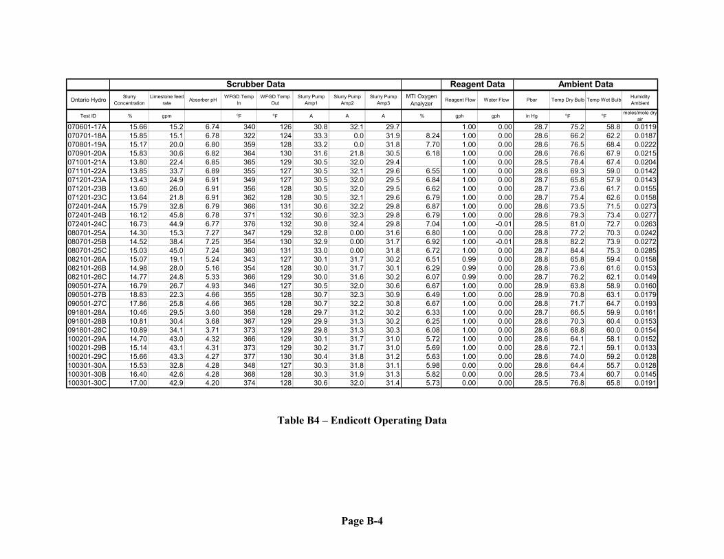
Page B-4

Ontario Hydro Slurry Concentration

Limestone feed rate Absorber pH WFGD Temp

InWFGD Temp

OutSlurry Pump

Amp1Slurry Pump

Amp2Slurry Pump

Amp3MTI Oxygen

Analyzer Reagent Flow Water Flow Pbar Temp Dry Bulb Temp Wet Bulb Humidity

Ambient

Test ID % gpm oF oF A A A % gph gph in Hg oF oFmoles/mole dry

air

070601-17A 15.66 15.2 6.74 340 126 30.8 32.1 29.7 1.00 0.00 28.7 75.2 58.8 0.0119070701-18A 15.85 15.1 6.78 322 124 33.3 0.0 31.9 8.24 1.00 0.00 28.6 66.2 62.2 0.0187070801-19A 15.17 20.0 6.80 359 128 33.2 0.0 31.8 7.70 1.00 0.00 28.6 76.5 68.4 0.0222070901-20A 15.83 30.6 6.82 364 130 31.6 21.8 30.5 6.18 1.00 0.00 28.6 76.6 67.9 0.0215071001-21A 13.80 22.4 6.85 365 129 30.5 32.0 29.4 1.00 0.00 28.5 78.4 67.4 0.0204071101-22A 13.85 33.7 6.89 355 127 30.5 32.1 29.6 6.55 1.00 0.00 28.6 69.3 59.0 0.0142071201-23A 13.43 24.9 6.91 349 127 30.5 32.0 29.5 6.84 1.00 0.00 28.7 65.8 57.9 0.0143071201-23B 13.60 26.0 6.91 356 128 30.5 32.0 29.5 6.62 1.00 0.00 28.7 73.6 61.7 0.0155071201-23C 13.64 21.8 6.91 362 128 30.5 32.1 29.6 6.79 1.00 0.00 28.7 75.4 62.6 0.0158072401-24A 15.79 32.8 6.79 366 131 30.6 32.2 29.8 6.87 1.00 0.00 28.6 73.5 71.5 0.0273072401-24B 16.12 45.8 6.78 371 132 30.6 32.3 29.8 6.79 1.00 0.00 28.6 79.3 73.4 0.0277072401-24C 16.73 44.9 6.77 376 132 30.8 32.4 29.8 7.04 1.00 -0.01 28.5 81.0 72.7 0.0263080701-25A 14.30 15.3 7.27 347 129 32.8 0.00 31.6 6.80 1.00 0.00 28.8 77.2 70.3 0.0242080701-25B 14.52 38.4 7.25 354 130 32.9 0.00 31.7 6.92 1.00 -0.01 28.8 82.2 73.9 0.0272080701-25C 15.03 45.0 7.24 360 131 33.0 0.00 31.8 6.72 1.00 0.00 28.7 84.4 75.3 0.0285082101-26A 15.07 19.1 5.24 343 127 30.1 31.7 30.2 6.51 0.99 0.00 28.8 65.8 59.4 0.0158082101-26B 14.98 28.0 5.16 354 128 30.0 31.7 30.1 6.29 0.99 0.00 28.8 73.6 61.6 0.0153082101-26C 14.77 24.8 5.33 366 129 30.0 31.6 30.2 6.07 0.99 0.00 28.7 76.2 62.1 0.0149090501-27A 16.79 26.7 4.93 346 127 30.5 32.0 30.6 6.67 1.00 0.00 28.9 63.8 58.9 0.0160090501-27B 18.83 22.3 4.66 355 128 30.7 32.3 30.9 6.49 1.00 0.00 28.9 70.8 63.1 0.0179090501-27C 17.86 25.8 4.66 365 128 30.7 32.2 30.8 6.67 1.00 0.00 28.8 71.7 64.7 0.0193091801-28A 10.46 29.5 3.60 358 128 29.7 31.2 30.2 6.33 1.00 0.00 28.7 66.5 59.9 0.0161091801-28B 10.81 30.4 3.68 367 129 29.9 31.3 30.2 6.25 1.00 0.00 28.6 70.3 60.4 0.0153091801-28C 10.89 34.1 3.71 373 129 29.8 31.3 30.3 6.08 1.00 0.00 28.6 68.8 60.0 0.0154100201-29A 14.70 43.0 4.32 366 129 30.1 31.7 31.0 5.72 1.00 0.00 28.6 64.1 58.1 0.0152100201-29B 15.14 43.1 4.31 373 129 30.2 31.7 31.0 5.69 1.00 0.00 28.6 72.1 59.1 0.0133100201-29C 15.66 43.3 4.27 377 130 30.4 31.8 31.2 5.63 1.00 0.00 28.6 74.0 59.2 0.0128100301-30A 15.53 32.8 4.28 348 127 30.3 31.8 31.1 5.98 0.00 0.00 28.6 64.4 55.7 0.0128100301-30B 16.40 42.6 4.28 368 128 30.3 31.9 31.3 5.82 0.00 0.00 28.5 73.4 60.7 0.0145100301-30C 17.00 42.9 4.20 374 128 30.6 32.0 31.4 5.73 0.00 0.00 28.5 76.8 65.8 0.0191

Scrubber Data Reagent Data Ambient Data


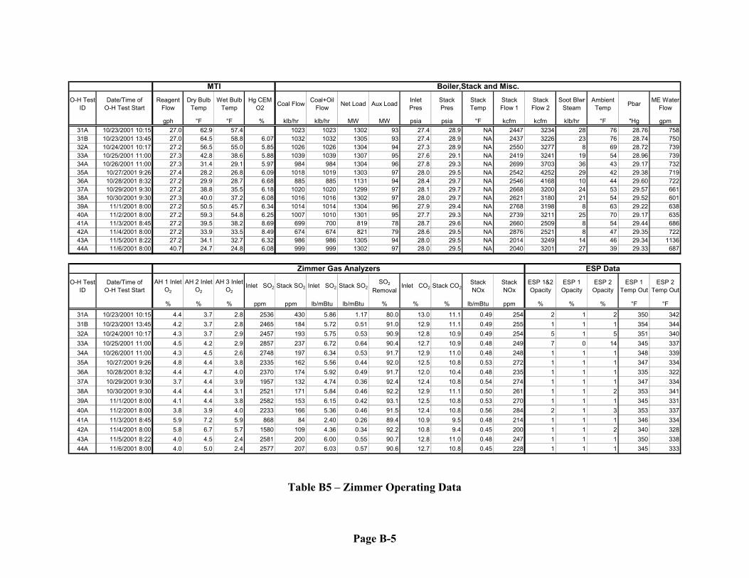
Page B-5

O-H Test ID

Date/Time of O-H Test Start

Reagent Flow

Dry Bulb Temp

Wet Bulb Temp

Hg CEM O2 Coal Flow Coal+Oil

Flow Net Load Aux Load Inlet Pres

Stack Pres

Stack Temp

Stack Flow 1

Stack Flow 2

Soot Blwr Steam

Ambient Temp Pbar ME Water

Flow

gph °F °F % klb/hr klb/hr MW MW psia psia °F kcfm kcfm klb/hr °F "Hg gpm31A 10/23/2001 10:15 27.0 62.9 57.4 1023 1023 1302 93 27.4 28.9 NA 2447 3234 28 76 28.76 75831B 10/23/2001 13:45 27.0 64.5 58.8 6.07 1032 1032 1305 93 27.4 28.9 NA 2437 3226 23 76 28.74 75032A 10/24/2001 10:17 27.2 56.5 55.0 5.85 1026 1026 1304 94 27.3 28.9 NA 2550 3277 8 69 28.72 73933A 10/25/2001 11:00 27.3 42.8 38.6 5.88 1039 1039 1307 95 27.6 29.1 NA 2419 3241 19 54 28.96 73934A 10/26/2001 11:00 27.3 31.4 29.1 5.97 984 984 1304 96 27.8 29.3 NA 2699 3703 36 43 29.17 73235A 10/27/2001 9:26 27.4 28.2 26.8 6.09 1018 1019 1303 97 28.0 29.5 NA 2542 4252 29 42 29.38 71936A 10/28/2001 8:32 27.2 29.9 28.7 6.68 885 885 1131 94 28.4 29.7 NA 2546 4168 10 44 29.60 72237A 10/29/2001 9:30 27.2 38.8 35.5 6.18 1020 1020 1299 97 28.1 29.7 NA 2668 3200 24 53 29.57 66138A 10/30/2001 9:30 27.3 40.0 37.2 6.08 1016 1016 1302 97 28.0 29.7 NA 2621 3180 21 54 29.52 60139A 11/1/2001 8:00 27.2 50.5 45.7 6.34 1014 1014 1304 96 27.9 29.4 NA 2768 3198 8 63 29.22 63840A 11/2/2001 8:00 27.2 59.3 54.8 6.25 1007 1010 1301 95 27.7 29.3 NA 2739 3211 25 70 29.17 63541A 11/3/2001 8:45 27.2 39.5 38.2 8.69 699 700 819 78 28.7 29.6 NA 2660 2509 8 54 29.44 68642A 11/4/2001 8:00 27.2 33.9 33.5 8.49 674 674 821 79 28.6 29.5 NA 2876 2521 8 47 29.35 72243A 11/5/2001 8:22 27.2 34.1 32.7 6.32 986 986 1305 94 28.0 29.5 NA 2014 3249 14 46 29.34 113644A 11/6/2001 8:00 40.7 24.7 24.8 6.08 999 999 1302 97 28.0 29.5 NA 2040 3201 27 39 29.33 687

O-H Test ID


AH 1 Inlet O2

AH 2 Inlet O2

AH 3 Inlet O2

Inlet SO2 Stack SO2 Inlet SO2 Stack SO2SO2

RemovalInlet CO2 Stack CO2

Stack NOx

Stack NOx

ESP 1&2 Opacity

ESP 1 Opacity

ESP 2 Opacity

ESP 1 Temp Out

ESP 2 Temp Out

% % % ppm ppm lb/mBtu lb/mBtu % % % lb/mBtu ppm % % % °F °F

31A 10/23/2001 10:15 4.4 3.7 2.8 2536 430 5.86 1.17 80.0 13.0 11.1 0.49 254 2 1 2 350 34231B 10/23/2001 13:45 4.2 3.7 2.8 2465 184 5.72 0.51 91.0 12.9 11.1 0.49 255 1 1 1 354 34432A 10/24/2001 10:17 4.3 3.7 2.9 2457 193 5.75 0.53 90.9 12.8 10.9 0.49 254 5 1 5 351 34033A 10/25/2001 11:00 4.5 4.2 2.9 2857 237 6.72 0.64 90.4 12.7 10.9 0.48 249 7 0 14 345 33734A 10/26/2001 11:00 4.3 4.5 2.6 2748 197 6.34 0.53 91.7 12.9 11.0 0.48 248 1 1 1 348 33935A 10/27/2001 9:26 4.8 4.4 3.8 2335 162 5.56 0.44 92.0 12.5 10.8 0.53 272 1 1 1 347 33436A 10/28/2001 8:32 4.4 4.7 4.0 2370 174 5.92 0.49 91.7 12.0 10.4 0.48 235 1 1 1 335 32237A 10/29/2001 9:30 3.7 4.4 3.9 1957 132 4.74 0.36 92.4 12.4 10.8 0.54 274 1 1 1 347 33438A 10/30/2001 9:30 4.4 4.4 3.1 2521 171 5.84 0.46 92.2 12.9 11.1 0.50 261 1 1 2 353 34139A 11/1/2001 8:00 4.1 4.4 3.8 2582 153 6.15 0.42 93.1 12.5 10.8 0.53 270 1 1 1 345 33140A 11/2/2001 8:00 3.8 3.9 4.0 2233 166 5.36 0.46 91.5 12.4 10.8 0.56 284 2 1 3 353 33741A 11/3/2001 8:45 5.9 7.2 5.9 868 84 2.40 0.26 89.4 10.9 9.5 0.48 214 1 1 1 346 33442A 11/4/2001 8:00 5.8 6.7 5.7 1580 109 4.36 0.34 92.2 10.8 9.4 0.45 200 1 1 2 340 32843A 11/5/2001 8:22 4.0 4.5 2.4 2581 200 6.00 0.55 90.7 12.8 11.0 0.48 247 1 1 1 350 33844A 11/6/2001 8:00 4.0 5.0 2.4 2577 207 6.03 0.57 90.6 12.7 10.8 0.45 228 1 1 1 345 333

ESP Data

MTI Boiler,Stack and Misc.

Zimmer Gas Analyzers

Table B5 – Zimmer Operating Data

Page B-6

O-H Test ID


Mod 1 Probe 1

Mod 1 Probe 2

Mod 2 Probe 1

Mod 2 Probe 2

Mod 3 Probe 1

Mod 3 Probe 2

Mod 4 Probe 1

Mod 4 Probe 2

Mod 5 Probe 1

Mod 5 Probe 2

Mod 6 Probe 1

Mod 6 Probe 2 Mod 1 Mod 2 Mod 3 Mod 4 Mod 5 Mod 6

pH pH pH pH pH pH pH pH pH pH pH pH % Sol % Sol % Sol % Sol % Sol % Sol

31A 10/23/2001 10:15 6.3 6.4 6.2 6.2 6.2 6.2 6.6 6.2 6.2 6.2 6.2 5.6 21 22 23 21 2331B 10/23/2001 13:45 6.5 6.6 6.5 6.5 6.8 6.5 6.5 6.5 6.9 6.4 22 23 21 23 2532A 10/24/2001 10:17 6.3 6.2 6.2 6.3 6.6 6.2 6.3 6.3 6.3 5.7 22 23 21 2333A 10/25/2001 11:00 6.4 6.4 6.4 6.3 6.7 6.4 6.4 6.4 6.3 5.7 22 23 21 23 2734A 10/26/2001 11:00 6.2 6.3 6.2 6.3 6.5 6.3 6.3 6.3 6.2 5.9 23 23 20 2435A 10/27/2001 9:26 6.2 6.2 6.2 6.2 6.4 6.2 6.2 6.2 6.2 6.2 24 21 24 20 2436A 10/28/2001 8:32 6.0 6.1 6.1 6.0 6.3 6.1 6.1 6.0 6.1 6.1 24 22 23 22 2337A 10/29/2001 9:30 6.1 6.2 6.4 6.4 6.5 6.2 6.2 6.2 6.2 6.2 22 23 22 23 2238A 10/30/2001 9:30 6.3 6.3 6.5 6.5 6.4 6.3 6.3 6.2 6.2 6.3 22 23 22 23 2339A 11/1/2001 8:00 6.4 6.5 6.4 6.5 6.6 6.2 6.4 6.3 6.5 6.6 22 22 22 21 1840A 11/2/2001 8:00 5.9 6.0 5.9 6.0 5.9 6.0 6.0 6.0 6.0 6.1 25 23 22 22 2241A 11/3/2001 8:45 6.0 6.0 6.0 6.1 6.1 6.1 6.1 6.0 6.1 6.0 25 24 22 22 1742A 11/4/2001 8:00 6.4 6.5 6.5 6.5 6.5 6.5 6.7 6.7 6.7 6.7 25 23 22 20 2343A 11/5/2001 8:22 6.4 6.5 6.3 6.3 6.6 6.5 6.2 6.2 6.5 6.5 16 23 22 19 3044A 11/6/2001 8:00 6.3 6.3 6.3 6.3 6.4 6.3 6.3 6.3 6.3 6.3 28 21 21 19 22

O-H Test ID

Date/Time of O-H Test Start Mod 1 Mod 2 Mod 3 Mod 4 Mod 5 Mod 6 Mod 1

InletMod 1 Outlet

Mod 2 Inlet

Mod 2 Outlet

Mod 3 Inlet

Mod 3 Outlet

Mod 4 Inlet

Mod 4 Outlet

Mod 5 Inlet

Mod 5 Outlet

Mod 6 Inlet

Mod 6 Outlet

Amps Amps Amps Amps Amps Amps °F °F °F °F °F °F °F °F °F °F °F °F

31A 10/23/2001 10:15 285 287 294 286 289 123 123 349 131 359 132 359 126 355 128 344 NA31B 10/23/2001 13:45 285 285 292 286 289 91 106 349 130 360 133 361 127 357 129 354 NA32A 10/24/2001 10:17 287 295 291 286 290 74 70 330 127 359 132 359 127 355 129 345 NA33A 10/25/2001 11:00 279 294 290 283 287 59 59 342 126 352 130 353 124 350 126 333 NA34A 10/26/2001 11:00 282 294 290 285 291 46 51 342 125 353 128 354 124 350 125 328 NA35A 10/27/2001 9:26 284 296 292 289 294 45 55 342 125 353 129 350 123 347 125 328 NA36A 10/28/2001 8:32 267 280 279 273 278 42 58 333 125 343 130 341 123 337 125 317 NA37A 10/29/2001 9:30 286 296 297 291 296 50 67 346 127 356 131 353 125 349 126 338 NA38A 10/30/2001 9:30 285 295 296 289 295 55 68 350 129 360 131 359 126 355 127 347 NA39A 11/1/2001 8:00 288 285 294 286 288 349 129 355 128 353 130 349 124 72 85 333 NA40A 11/2/2001 8:00 293 290 299 289 291 355 131 361 131 360 131 355 126 72 69 340 NA41A 11/3/2001 8:45 252 247 252 248 251 349 126 355 125 351 127 354 121 60 58 325 NA42A 11/4/2001 8:00 251 247 252 246 249 346 125 351 124 348 127 350 121 54 54 319 NA43A 11/5/2001 8:22 287 279 292 281 282 356 129 361 127 358 128 353 125 56 55 328 NA44A 11/6/2001 8:00 289 283 295 283 285 349 131 355 128 352 129 344 123 52 54 322 NA

WFGD Inlet/Outlet Temperature

WFGD Tray pH WFGD Slurry % Solids

WFGD ID Fan Amps


Page B-7

O-H Test ID


Mod 1 Pump 1

Mod 1 Pump 2

Mod 2 Pump 1

Mod 2 Pump 2

Mod 3 Pump 1

Mod 3 Pump 2

Mod 4 Pump 1

Mod 4 Pump 2

Mod 5 Pump 1

Mod 5 Pump 2

Mod 6 Pump 1

Mod 6 Pump 2 Mod 1 Mod 2 Mod 3 Mod 4 Mod 5 Mod 6

Amps Amps Amps Amps Amps Amps Amps Amps Amps Amps Amps Amps "H2O "H2O "H2O "H2O "H2O "H2O

31A 10/23/2001 10:15 36 39 37 34 37 36 0.9 2.5 2.5 2.1 2.0 1.731B 10/23/2001 13:45 39 36 33 37 37 0.9 2.5 2.5 2.0 2.1 1.832A 10/24/2001 10:17 39 37 34 37 37 2.5 2.7 1.7 2.0 1.733A 10/25/2001 11:00 40 37 34 38 36 2.4 2.7 1.6 2.0 1.734A 10/26/2001 11:00 39 37 34 38 37 2.4 2.6 1.8 2.1 1.735A 10/27/2001 9:26 39 37 34 37 37 2.4 2.7 1.8 2.1 1.736A 10/28/2001 8:32 39 37 34 38 38 2.1 2.4 1.8 1.8 1.537A 10/29/2001 9:30 40 37 34 37 38 2.5 2.6 1.7 2.1 1.738A 10/30/2001 9:30 39 37 34 37 38 2.5 2.6 1.7 2.1 1.739A 11/1/2001 8:00 29 32 39 32 38 34 29 33 2.6 2.5 3.0 1.7 1.840A 11/2/2001 8:00 29 33 40 35 37 34 35 3.1 2.6 3.0 1.7 1.641A 11/3/2001 8:45 36 40 37 34 33 1.7 1.9 1.9 1.2 1.242A 11/4/2001 8:00 27 32 39 37 33 34 1.5 1.8 1.9 1.3 1.243A 11/5/2001 8:22 32 38 37 34 34 2.2 2.5 2.8 2.2 1.644A 11/6/2001 8:00 33 32 35 37 32 34 29 34 2.7 2.8 2.8 2.1 1.8

WFGD Slurry Recirculation Pump Amps WFGD Differential Pressure


Documents

Full-Scale Testing of Enhanced Mercury Control ... Library/Research/Coal/ewr/mercury... · FULL-SCALE TESTING OF ENHANCED MERCURY CONTROL TECHNOLOGIES FOR WET FGD SYSTEMS Final Report