FunConn v1 User’s Manual: ArcGIS tools for Functional ...nsu/starmap/learningmaterials/technical... · ArcGIS tools for Functional Connectivity Modeling ... FunConn v1 User’s

FunConn v1 Users Guide

FunConn v1 User’s Manual: ArcGIS tools for Functional Connectivity Modeling Authors: David M. Theobald John B. Norman Melissa R. Sherburne Contact info: Natural Resource Ecology Laboratory Colorado State University Fort Collins, CO 80523 www.nrel.colostate.edu/projects/[email protected] Funding/Disclaimer: The work reported here was developed under the STAR Research Assistance Agreement CR-829095 awarded by the U.S. Environmental Protection Agency (EPA) to Colorado State University. This document has not been formally reviewed by EPA. EPA does not endorse any products mentioned here. Citation:

Page 1 - 7/26/2006

Theobald, D.M., J.B. Norman, M.R. Sherburne. 2006. FunConn v1 User’s Manual: ArcGIS tools for Functional Connectivity Modeling. Natural Resource Ecology Lab, Colorado State University, Fort Collins, CO.

http://www.nrel.colostate.edu/projects/starmap

mailto:[email protected]


Abstract The FunConn (pronounced ‘funkin’) modeling toolbox for ArcGIS v9 provides graph theoretic-based analysis methods for landscape connectivity and offers substantial extensions to traditional least-cost path approaches. Conservation practitioners should embrace this innovative approach for several reasons:

The graph/landscape network data structure allows for an elegant, computationally efficient representation of a landscape. Complex landscapes can be modeled across large regions, encompassing thousands of habitat patches, without compromising fine-grain spatial variation.

Users can evaluate landscape-level connectivity, between all patches, not simply adjacent patches (1st order neighbors). This is a valuable way to identify ‘bottlenecks’- locations that are critical for overall connectivity due to the spatial configuration of habitat (not simply the influence of immediate neighborhood context).

Graph edges (landscape network linkages and corridors) can have user-defined weight attributes; providing flexibility in calculating a variety of graph-based landscape metrics such as, patch area, corridor width, and average cost distance.

In short, the graph theoretic approach to modeling landscape connectivity is more flexible, efficient, and more powerful than traditional least-cost-path analysis. This document provides an overview of FunConn’s two primary toolsets: Habitat Modeling and Landscape Networks. The Habitat Modeling toolset was designed for those who want to generate a terrestrial habitat quality raster, functional patches, and a landscape network from the ground up. Because the habitat model is based on species-vegetation affinities, the data requirements are minimal: in addition to landcover, no existing sampling data are required. The Landscape Network toolset is designed for those interested in generating a landscape network based on existing data, or analyzing an existing landscape network. It contains three sub-toolsets: Processing, Analysis, and Export. The Processing toolset generates the landscape network based on points, polygons, or polylines. The Analysis toolset allows for graph theoretic or network-type analyses to be executed on landscape networks. The Habitat Modeling landscape network is suitable for analysis within this toolset. Tools included in the Analysis toolset allow for calculating minimum spanning trees based on a user-defined weight values, calculating node and edge interactions based on user-defined fields and equation strings, and finding the shortest paths from each node to every other node in the network. The Export toolset exports the landscape network to an NxN matrix based on user-defined weight values. An example dataset is provided so you can become familiar with the FunConn concepts and tools before applying them to your datasets. These data are in the lynx folder; save this to your local drive.

Page 2 - 7/26/2006


TABLE OF CONTENTS Software Environment 3 Example Dataset 3 Terminology 5 Feature Class Attributes 8 PART 1: HABITAT MODELING TOOLSET 10 I. Create Habitat Quality 11 II. Define Functional Patches 21 III. Build Landscape Network 24 PART 2: LANDSCAPE NETWORKS TOOLSET 29 I. Processing 30 Points to Landscape Network 30 Polygons to Landscape Network 31 Polyline to Landscape Network 32 II. Analysis 33 Minimum Spanning Tree 33 Edge Calculator 34 Neighborhood Selection 36 Node Calculator 37 Shortest Paths 40 III. Export 42 Node-Edge-Node Distance Matrix (D) 42 Node-Path-Node Distance Matrix (D') 43 References 44 Appendix 45 Methods for Creating a Disturbance Raster 45 Geoprocessing Steps Overview Diagram 48

Page 3 - 7/26/2006


Software Environment FunConn tools were written within Python (v2.1) as a Geoprocessing toolbox and ArcGIS v9.1. An ArcINFO level license is required to run certain FunConn tools in which a personal geodatabase is created, which are: the Habitat Modeling/Build Landscape Network Tool and the Landscape Networks/Processing Tools.. Once a landscape network is created, all other tools can run using either an ArcView or ArcINFO license. The FunConn tools also require the Spatial Analyst extension. Before using the FunConn tools, be sure to have the Spatial Analyst extension activated and a c:\temp directory on your machine - this is where output directories are stored. All input data should be in the same projected coordinate system and datum. To use the Habitat Modeling tools, you must have a land cover dataset for your study area. All of the additional parameters are user-defined and explained in this guide. Example Dataset Description The following datasets are found in the lynx folder provided with the FunConn Tools. Save this folder to your local drive exactly as c:\lynx to avoid model failure due to ESRI character limits*. Use this dataset to run example models or to compare with your results. Name Format Definition vp_swrgp raster southwest regional gap land cover data for vail pass area

vp_disturb raster southwest regional gap land cover data for vail pass area w/ disturbance

vp_slope_cost raster additional cost raster- slope

vp_area* raster example area boundary

habitat_quality .dbf habitat quality reclass table

disturbance .dbf disturbance reclass table

patch_structure .dbf patch structure reclass table

permeability .dbf permeability reclass table

vail_pass_counties** shapefile counties

vail_pass_highways** shapefile highways

vail_pass_towns** shapefile towns

lynx\results\ex_hq*** raster completed example habitat quality raster

lynx\results\ex_patches*** raster completed example patches raster

lynx\results\ex_network*** raster completed example landscape network

*ESRI’s character limit for conditional statements is 4000. Long path names or a large number of classes can cause this to be exceeded. **Non-essential for running the FunConn tools, but are provided for reference purposes only. ***These are examples of successful tool completion (using the default parameters and example tables); use for comparison against the results of your operations.

Page 4 - 7/26/2006


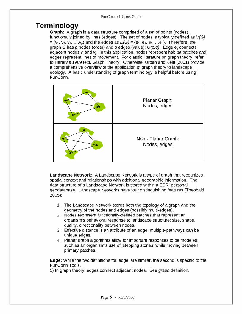
Terminology Graph: A graph is a data structure comprised of a set of points (nodes) functionally joined by lines (edges). The set of nodes is typically defined as V(G) = {v1, v2, v3, ….vp} and the edges as E(G) = {e1, e2, e3, …eq}. Therefore, the graph G has p nodes (order) and q edges (value): G(p,q). Edge eij connects adjacent nodes vi and vj. In this application, nodes represent habitat patches and edges represent lines of movement. For classic literature on graph theory, refer to Harary’s 1969 text, Graph Theory. Otherwise, Urban and Keitt (2001) provide a comprehensive overview of the application of graph theory to landscape ecology. A basic understanding of graph terminology is helpful before using FunConn.

Landscape Network: A Landscape Network is a type of graph that recognizes spatial context and relationships with additional geographic information. The data structure of a Landscape Network is stored within a ESRI personal geodatabase. Landscape Networks have four distinguishing features (Theobald 2005):

1. The Landscape Network stores both the topology of a graph and the geometry of the nodes and edges (possibly multi-edges).

2. Nodes represent functionally-defined patches that represent an organism’s behavioral response to landscape structure: size, shape, quality, directionality between nodes.

3. Effective distance is an attribute of an edge; multiple-pathways can be unique edges.

4. Planar graph algorithms allow for important responses to be modeled, such as an organism’s use of ‘stepping stones’ while moving between primary patches.

Edge: While the two definitions for ‘edge’ are similar, the second is specific to the FunConn Tools. 1) In graph theory, edges connect adjacent nodes. See graph definition.

Page 5 - 7/26/2006

Non - Planar Graph: Nodes, edges

Planar Graph: Nodes, edges


2) The edges generated by the FunConn Tools are stored within the Landscape Network connect nodes centroid-to-centroid, are not straight-line, and have a one to many relationship with node pairs (multi-edge). Also, each edge is represented twice in the relationship table to account for directionality. The Landscape Network edges contain the following attributes: edge length, effective distances, centroid-to-centroid angle, and mean angle vector. Node: In a graph, a node is a point functionally connected to other points via edges. Nodes are stored in the Landscape Network as a point feature class. However, patches defined by a polygon feature class can also serve as nodes in the FunConn Landscape Network Analysis tools. Linkage: Linkages are the least-cost pathways between patch edges defined by cost allocation boundaries and a certain threshold that allows for multiple-linkages to be defined. This threshold is set through the qn value which is user-defined in the Create Landscape Network tool. Also, each linkage is represented twice in the relationship table to account for directionality. Patch: A habitat area functionally defined by habitat quality, size, and proximity constraints. In a traditional graph, patch centers serve as the nodes connected by straight-line edges. In a Landscape Network, the patches are stored as a polygon feature class, and linkages originate at the patch perimeter. Corridor: A representation of the optimal movement pathway between adjacent habitat patches. Corridors have a one-to-many relationship between node pairs; one corridor can connect several patches. The geometry of the corridors reveals potential geographic “bottlenecks” or other shape characteristics that might enhance or inhibit the traversability of a habitat network. Cluster: A group of patches that function as a single patch. Path: A walk in which all nodes and edges are unique. If a path has more than 3 nodes, with no cycles, it is a tree. Walk: A sequence of nodes connected by edges. If a walk ends at the first node, it is a cycle. Core Seed: An area of high-quality habitat from which the functional patches originate. From the seed, the patches are ‘grown’ across a cost surface to a distance equal to the units of the foraging radius. See Define Functional Patches tool. Model: The definition of a ‘model’ depends on its context: 1) Simulation of a process or response at a given scale. For example, lynx natal dispersal across a landscape, i.e.: lynx habitat model. v., modeling. 2) In ArcGIS geoprocessing, a process or series of linked processes represented by a flow diagram in Modelbuilder.

Page 6 - 7/26/2006

Tool: A tool is a Python script found in a toolset. The Habitat Modeling toolset contains 3 tools: Create Habitat Quality, Define Functional Patches, and Build Landscape Network. The Landscape Network/Processing toolset contains 3


tools: Points to Landscape Network, Polygon to Landscape Network, and Polyline to Landscape Network. The Landscape Network/Analysis toolset contains 5 tools: Calculate Minimum Spanning Tree, Edge Calculator, Node Calculator, Neighborhood Selection, and Shortest Paths. Toolbox: The entire collection of FunConn toolsets and tools.

Page 7 - 7/26/2006

Toolset: FunConn contains 2 primary toolsets: Habitat Modeling and Landscape Networks. The Landscape Network toolset contains 3 sub-toolsets: Processing, Analysis, and Export.


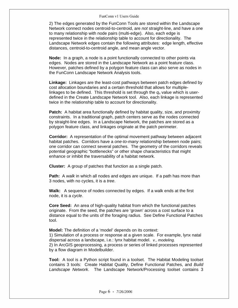
FEATURE CLASS ATTRIBUTES (For Edges, Linkages, and Corridors) *Standard attributes such as Object ID, FID, Shape, Area, and Perimeter are omitted.

Edges

qn Fields (q5, q10, q25, q50, qmin, qmean): The value for that line, below which qn values fall. Shape_Length: The Euclidean distance from centroid-midpoint-centroid. Straight_Dist: The Euclidean distance from centroid-to-centroid, without crossing through the midpoint qn values. C2C_Angle: Centroid-to-centroid angle. Mean_Angle_Vect: The average angle across all edge segments.

Linkages

qn Fields (q5, q10, q25, q50, qmin, qmean): The value for that line, below which qn values fall. Shape_Length: The Euclidean distance from centroid-midpoint-centroid. Straight_Dist: The Euclidean distance from centroid-to-centroid, without crossing through the midpoint qn values. B2B_Angle: Boundary-to-boundary angle. Mean_Angle_Vect: The average angle across all edge segments.

Corridors

Area: Area of the corridor, calculated in map units. Perimeter: Length of the entire corridor boundary. Topo_num: Topological number is the number of patches that connect via that corridor. One corridor can connect many patches.

Page 8 - 7/26/2006

Corridors

Linkages

Edges


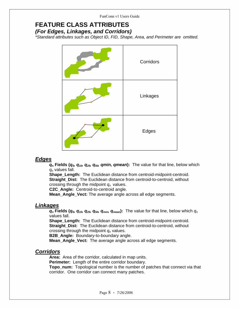
From_SharBound: The width of the corridor where it intersects the from_patch boundary. To_SharBound: The width of the corridor where it intersects the to_patch boundary. Mid_SharBound: The width of the corridor at the center-most point of the corridor.

Page 9 - 7/26/2006

Topo_num = 2 Topo_num = 3 Topo_num = 2


PART 1: Habitat Modeling Toolset

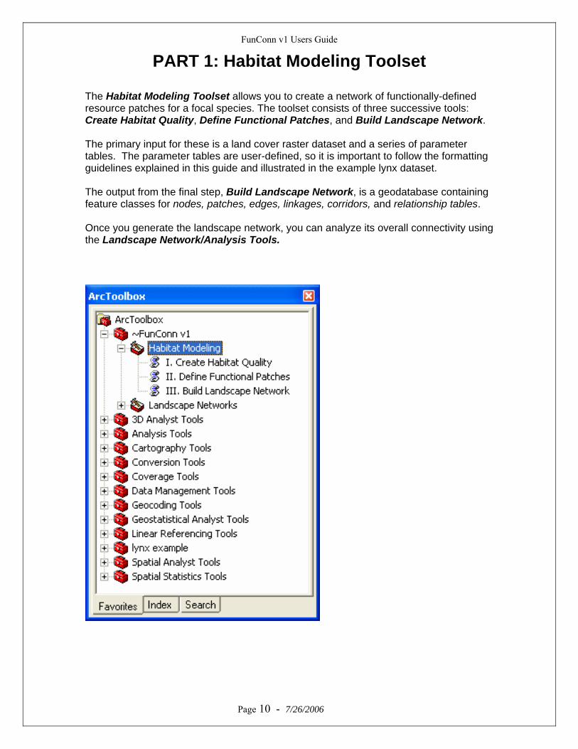
The Habitat Modeling Toolset allows you to create a network of functionally-defined resource patches for a focal species. The toolset consists of three successive tools: Create Habitat Quality, Define Functional Patches, and Build Landscape Network. The primary input for these is a land cover raster dataset and a series of parameter tables. The parameter tables are user-defined, so it is important to follow the formatting guidelines explained in this guide and illustrated in the example lynx dataset. The output from the final step, Build Landscape Network, is a geodatabase containing feature classes for nodes, patches, edges, linkages, corridors, and relationship tables. Once you generate the landscape network, you can analyze its overall connectivity using the Landscape Network/Analysis Tools.

Page 10 - 7/26/2006


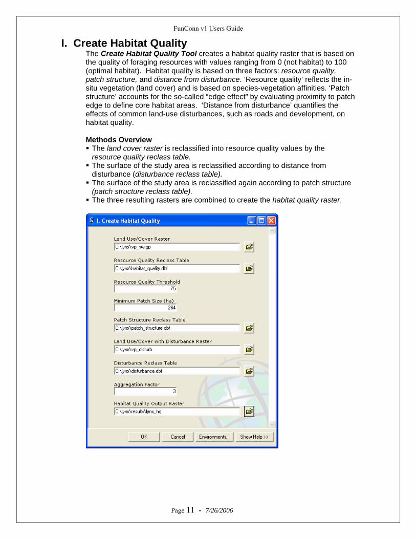
I. Create Habitat Quality The Create Habitat Quality Tool creates a habitat quality raster that is based on the quality of foraging resources with values ranging from 0 (not habitat) to 100 (optimal habitat). Habitat quality is based on three factors: resource quality, patch structure, and distance from disturbance. ‘Resource quality’ reflects the in-situ vegetation (land cover) and is based on species-vegetation affinities. ‘Patch structure’ accounts for the so-called “edge effect” by evaluating proximity to patch edge to define core habitat areas. ‘Distance from disturbance’ quantifies the effects of common land-use disturbances, such as roads and development, on habitat quality. Methods Overview The land cover raster is reclassified into resource quality values by the resource quality reclass table.

The surface of the study area is reclassified according to distance from disturbance (disturbance reclass table).

The surface of the study area is reclassified again according to patch structure (patch structure reclass table).

The three resulting rasters are combined to create the habitat quality raster.

Page 11 - 7/26/2006


Parameters Land Cover Raster Specify the land cover raster that represents the landscape to be used by your organism. This can be USGS NLCD, USGS GAP, or user-defined, but must be in raster format and be categorical or class (nominal) data. The example raster is c:\lynx\vp_swrgp and is derived from the Southwest Regional GAP data (http://fws-nmcfwru.nmsu.edu/swregap/). There is a 4000 character limit within ArcGIS software for the raster conditional statement used within this tool. If the file or path name is too long, or if your raster has a large number of classes (such as Southwest ReGap with ~125) this may cause this tool or process to fail because the conditional statement exceeds the 4000 character limit. To avoid this problem, save your land cover and disturbance rasters directly in c:\ or c:\temp with short file names, and/or, reduce the number of classes in your land cover dataset. Resource Quality Reclass Table This table contains the data necessary to reclassify the land cover raster into habitat quality values for each organism. Format:

*.dbf table. Required Fields: Case Sensitive

1. GRIDCODE- short or long integer type, 0 decimal places; land cover grid value.

2. QUALITY- short or long integer type, 0 decimal places; organism-specific; value range 0 (not habitat) – 100 (optimal habitat quality).

Example Table:

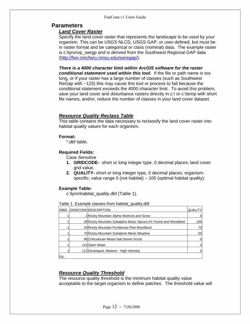
c:\lynx\habitat_quality.dbf (Table 1). Table 1. Example classes from habitat_quality.dbf. OBID GRIDCODE DESCRIPTION QUALITY

1 2 Rocky Mountain Alpine Bedrock and Scree 0

1 28 Rocky Mountain Subalpine Mesic Spruce-Fir Forest and Woodland 100

1 34 Rocky Mountain Ponderosa Pine Woodland 70

1 70 Rocky Mountain Subalpine Mesic Meadow 50

1 96 Chihuahuan Mixed Salt Desert Scrub 0

1 110 Open Water 0

1 112 Developed, Medium - High Intensity 0

Etc.

Resource Quality Threshold

Page 12 - 7/26/2006

The resource quality threshold is the minimum habitat quality value acceptable to the target organism to define patches. The threshold value will

http://fws-nmcfwru.nmsu.edu/swregap/


typically fall near 75-80 (range 0-100), and is based on the QUALITY values from the Resource Quality Reclass Table. The default value is 75 and represents a minimum habitat quality of 75% acceptability to the organism, where 100% is the best possible habitat. This does not mean that any land cover cell that is below the threshold will be eliminated (see next paragraph). The resource quality threshold is used twice in the Habitat Modeling processes. The first use establishes the primary habitat areas from which to base smaller ‘stepping-stone’ habitat areas and ultimately the seeds for defining functional patches. While you are setting a threshold for retaining areas of a certain habitat quality, areas of lower habitat quality will not be eliminated until their relationship (based on distance) to the primary patches is evaluated. This is done through the patch structure reclass table. Minimum Patch Size (ha) Enter the minimum patch size (in hectares) to be evaluated. This threshold is the smallest biologically relevant patch size for the target organism. It may be based on known home range sizes or by estimating home range size using allometric relationships between body mass and home range size (Jetz et al. 2004). To ensure that the full range of possible home range sizes is covered, we recommend running the model at an order of magnitude less than and greater than the estimated home range size. The minimum patch size for the example lynx is 264 ha. See Appendix: Geoprocessing Steps for details on how this parameter is incorporated into the model. Patch Structure Reclass Table

Page 13 - 7/26/2006

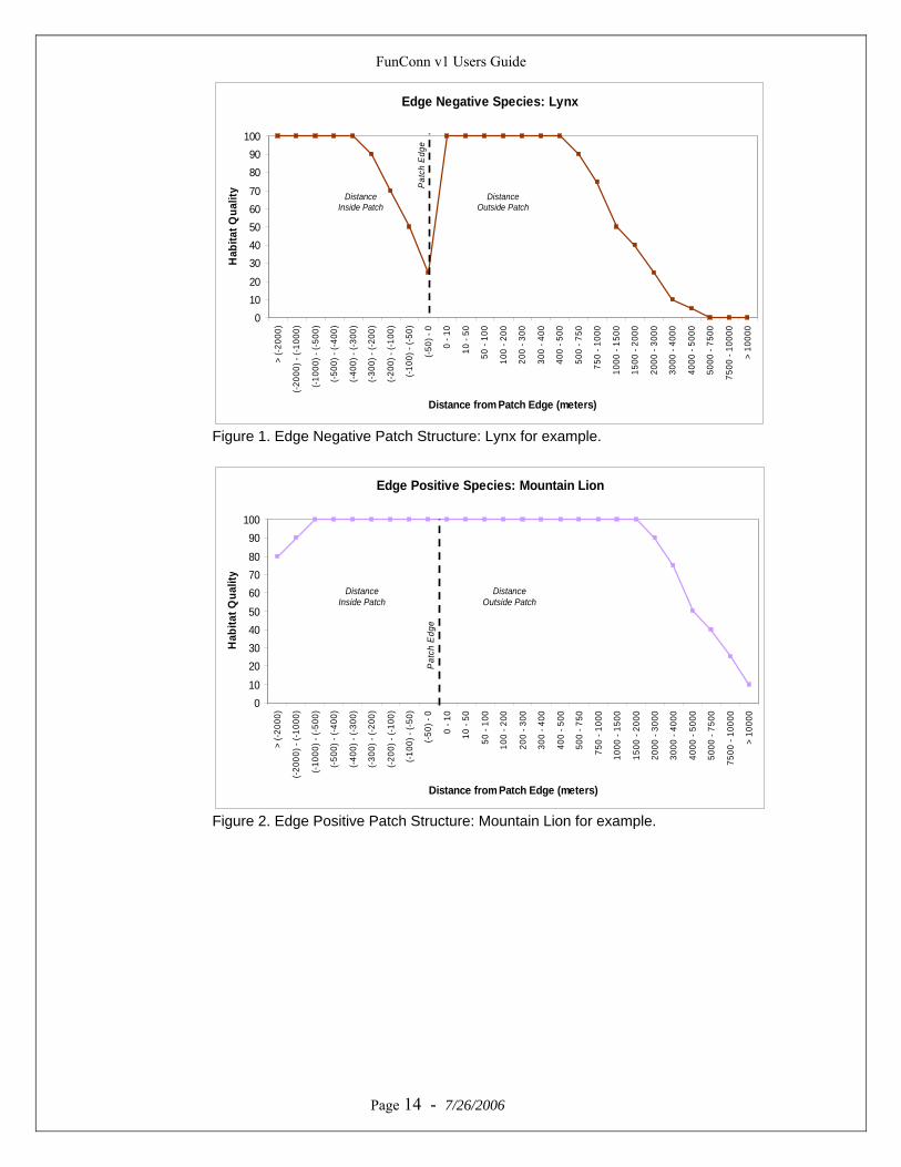
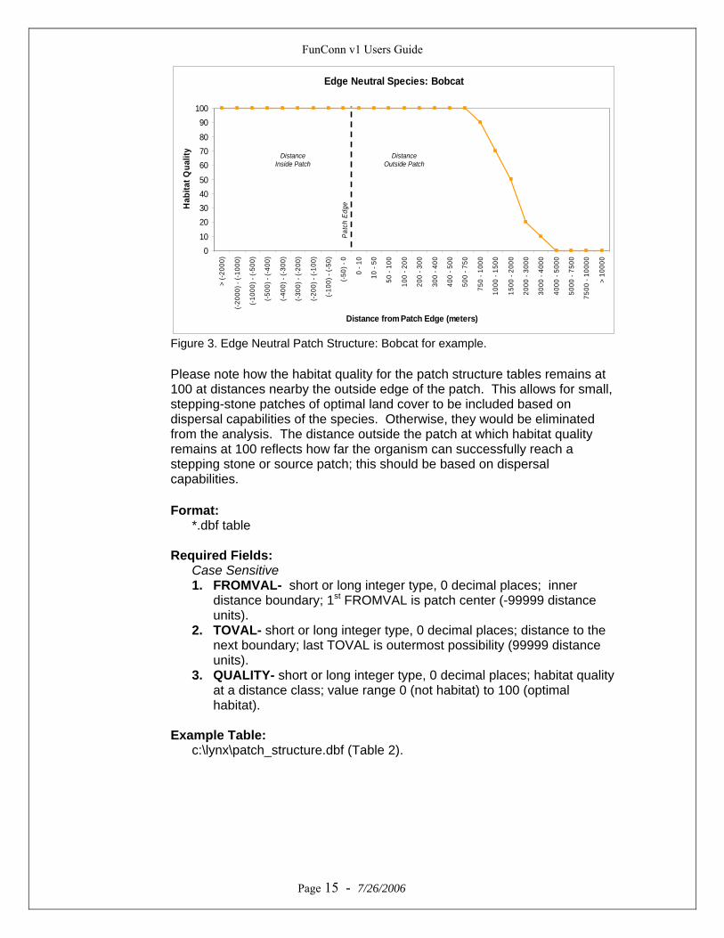
This table contains the data necessary to define an organism’s response to edge and core habitats. For instance, if a patch is composed of entirely of high-quality land cover type, does it decrease in value as the organism approaches the edge? In the case of lynx, an old growth spruce-fir patch is optimal; however the core of the patch is more valuable than the edge. These core-favoring species are edge-negative (Figure 1). Other species, such as mountain lion, might prefer edge areas due to their hunting practices. The patch structure table would reflect that by having slightly lower habitat quality values for the inner-most area of the patch. These species are edge-positive (Figure 2). Species that exhibit no preference for core or edge habitat areas are edge-neutral (Figure 3).


Edge Negative Species: Lynx

01020

3040506070

8090

100

> (-

2000

)

(-20

00) -

(-10

00)

(-100

0) -

(-50

0)

(-50

0) -

(-40

0)

(-40

0) -

(-30

0)

(-30

0) -

(-20

0)

(-20

0) -

(-10

0)

(-10

0) -

(-50

)

(-50

) - 0

0 - 1

0

10 -

50

50 -

100

100

- 200

200

- 300

300

- 400

400

- 500

500

- 750

750

- 100

0

1000

- 15

00

1500

- 20

00

2000

- 30

00

3000

- 40

00

4000

- 50

00

5000

- 75

00

7500

- 10

000

> 10

000

Distance from Patch Edge (meters)

Hab

itat Q

ualit

y Pat

ch E

dge

DistanceInside Patch

DistanceOutside Patch

Figure 1. Edge Negative Patch Structure: Lynx for example.

Edge Positive Species: Mountain Lion

010

20304050

607080

90100

> (-2

000)

(-200

0) -

(-100

0)

(-10

00) -

(-50

0)

(-500

) - (-

400)

(-400

) - (-

300)

(-300

) - (-

200)

(-200

) - (-

100)

(-100

) - (-

50)

(-50)

- 0

0 - 1

0

10 -

50

50 -

100

100

- 200

200

- 300

300

- 400

400

- 500

500

- 750

750

- 100

0

1000

- 15

00

1500

- 20

00

2000

- 30

00

3000

- 40

00

4000

- 50

00

5000

- 75

00

7500

- 10

000

> 10

000


Hab

itat Q

ualit

y

Pat

ch E

dge



Figure 2. Edge Positive Patch Structure: Mountain Lion for example.

Page 14 - 7/26/2006


Edge Neutral Species: Bobcat

010

20304050

607080

90100

> (-

2000

)

(-20

00) -

(-10

00)

(-10

00) -

(-50

0)

(-50

0) -

(-40

0)

(-40

0) -

(-30

0)

(-30

0) -

(-20

0)

(-20

0) -

(-10

0)

(-10

0) -

(-50

)

(-50

) - 0

0 - 1

0

10 -

50

50 -

100

100

- 200

200

- 300

300

- 400

400

- 500

500

- 750

750

- 100

0

1000

- 15

00

1500

- 20

00

2000

- 30

00

3000

- 40

00

4000

- 50

00

5000

- 75

00

7500

- 10

000

> 10

000


Hab

itat Q

ualit

y

Pat

ch E

dge



Figure 3. Edge Neutral Patch Structure: Bobcat for example.

Please note how the habitat quality for the patch structure tables remains at 100 at distances nearby the outside edge of the patch. This allows for small, stepping-stone patches of optimal land cover to be included based on dispersal capabilities of the species. Otherwise, they would be eliminated from the analysis. The distance outside the patch at which habitat quality remains at 100 reflects how far the organism can successfully reach a stepping stone or source patch; this should be based on dispersal capabilities.

Format:

*.dbf table Required Fields: Case Sensitive

1. FROMVAL- short or long integer type, 0 decimal places; inner distance boundary; 1st FROMVAL is patch center (-99999 distance units).

2. TOVAL- short or long integer type, 0 decimal places; distance to the next boundary; last TOVAL is outermost possibility (99999 distance units).

3. QUALITY- short or long integer type, 0 decimal places; habitat quality at a distance class; value range 0 (not habitat) to 100 (optimal habitat).

Example Table:

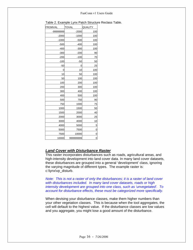
c:\lynx\patch_structure.dbf (Table 2).

Page 15 - 7/26/2006


Table 2. Example Lynx Patch Structure Reclass Table. FROMVAL TOVAL QUALITY

-99999999 -2000 100

-2000 -1000 100

-1000 -500 100

-500 -400 100

-400 -300 100

-300 -200 90

-200 -100 70

-100 -50 50

-50 0 25

0 10 100

10 50 100

50 100 100

100 200 100

200 300 100

300 400 100

400 500 100

500 750 90

750 1000 75

1000 1500 50

1500 2000 40

2000 3000 25

3000 4000 10

4000 5000 5

5000 7500 0

7500 10000 0

10000 999999999 0

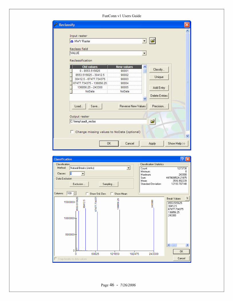
Land Cover with Disturbance Raster This raster incorporates disturbances such as roads, agricultural areas, and high-intensity development into land cover data. In many land cover datasets, these disturbances are grouped into a general ‘development’ class, ignoring the varying magnitude of different types. The example raster is: c:\lynx\vp_disturb. Note: This is not a raster of only the disturbances; it is a raster of land cover with disturbances included. In many land cover datasets, roads or high intensity development are grouped into one class, such as ‘unvegetated’. To account for disturbance effects, these must be categorized more specifically. When devising your disturbance classes, make them higher numbers than your other vegetation classes. This is because when the tool aggregates, the cell will default to the highest value. If the disturbance classes are low values and you aggregate, you might lose a good amount of the disturbance.

Page 16 - 7/26/2006


One possible technique for creating this dataset is to embed the disturbances into the land cover dataset. To do this, first classify the roads into ~5 classes based on road type (highway, local road, etc.) or by traffic volume (Average Annual Daily Traffic, AADT). Next, convert the roads into a raster by road class. Lastly, use a conditional statement to replace the original land cover values with the disturbance grid values. The example dataset classifies disturbances as classes 90001 – 90005 by AADT and high-intensity development (Table 3).

Table 3. Example Lynx Disturbance Classification.

Assigned Value Class

90001 0 - 5K AADT 90002 5K - 10K AADT 90003 10K - 30K AADT 90004 >30K AADT 90005 High-intensity development

When devising your disturbance classes, make them higher numbers than your other vegetation classes. This is because when the tool aggregates, the cell will default to the highest value. If the disturbance classes are low values and you aggregate, you might lose a good amount of the disturbance. See Appendix: Methods for Creating the Landcover with Disturbance Raster.

Disturbance Reclass Table Avoidance of roads by organisms, especially due to traffic, has importance ecological impacts (Forman and Alexander 1998). This reclass table attempts to capture these impacts by measuring the effect of a disturbance at given distances. The table’s values range from 0 (total habitat quality loss or 0% quality retained) to 100 (no effect on habitat quality or 100% quality retained). For some initial guidance on quantifying your focal species’ sensitivity to roads, refer to Richard T.T. Formans text, Road Ecology: Science and Solutions. Format:


1. FROMVAL- inner distance boundary; originates at the disturbance center (-99999 distance units, e.g. meters).

2. TOVAL- outer boundary distance; outermost is the furthest possibility (99999 distance units).

Page 17 - 7/26/2006

3. V<classes>- User-defined disturbance class that corresponds with the disturbance class; must add a “V” preceding the class ID (i.e.: if


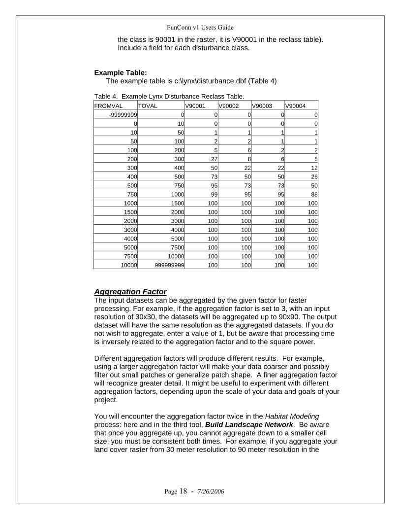
the class is 90001 in the raster, it is V90001 in the reclass table). Include a field for each disturbance class.

Example Table:

The example table is c:\lynx\disturbance.dbf (Table 4) Table 4. Example Lynx Disturbance Reclass Table. FROMVAL TOVAL V90001 V90002 V90003 V90004

-99999999 0 0 0 0 0 0 10 0 0 0 0

10 50 1 1 1 1 50 100 2 2 1 1

100 200 5 6 2 2 200 300 27 8 6 5 300 400 50 22 22 12 400 500 73 50 50 26 500 750 95 73 73 50 750 1000 99 95 95 88

1000 1500 100 100 100 100 1500 2000 100 100 100 100 2000 3000 100 100 100 100 3000 4000 100 100 100 100 4000 5000 100 100 100 100 5000 7500 100 100 100 100 7500 10000 100 100 100 100

10000 999999999 100 100 100 100

Aggregation Factor The input datasets can be aggregated by the given factor for faster processing. For example, if the aggregation factor is set to 3, with an input resolution of 30x30, the datasets will be aggregated up to 90x90. The output dataset will have the same resolution as the aggregated datasets. If you do not wish to aggregate, enter a value of 1, but be aware that processing time is inversely related to the aggregation factor and to the square power. Different aggregation factors will produce different results. For example, using a larger aggregation factor will make your data coarser and possibly filter out small patches or generalize patch shape. A finer aggregation factor will recognize greater detail. It might be useful to experiment with different aggregation factors, depending upon the scale of your data and goals of your project.

Page 18 - 7/26/2006

You will encounter the aggregation factor twice in the Habitat Modeling process: here and in the third tool, Build Landscape Network. Be aware that once you aggregate up, you cannot aggregate down to a smaller cell size; you must be consistent both times. For example, if you aggregate your land cover raster from 30 meter resolution to 90 meter resolution in the


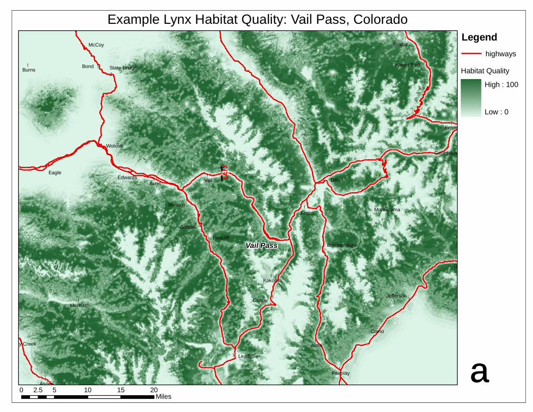
Create Habitat Quality Tool, you cannot decide to change this to 60 meter resolution in the Build Landscape Network Tool. If you foresee wanting to have an multiple landscape networks at different scales, the best approach would be to generate your Habitat Quality and Patches rasters at the finest grain (e.g., 30 meters) and use different aggregations in the Build Landscape Network Tool. It is beneficial to test different aggregation factors on a sample area of your study area before deciding on the best one. Habitat Quality Output Raster Specify the name and location of the output raster. This raster is the input for the next tool, Define Functional Patches. The example output is c:\lynx\Results\habitat_quality. The habitat quality directory is created using “hq” following with a time-stamp: c:\temp\hq_<yyymmddhhmmss>. This time-stamp directory contains a variety of temporary rasters, although the final habitat quality raster is saved in the location that you specify. See the readme file in the hq directory folder for a description of its contents. Within the time-stamp folder is a README file with the parameter specifications of the model run.

Page 19 - 7/26/2006

!

!

!

!

!

!

!

!

!

!

!

!

!

!

!

!

!

!

!

!

!

!

!

!!

!

!

!

!

!

!Vail

Como

Bond

Avon

Alma

McCoy

Grant

Eagle

Burns

Aspen

Kokomo

Gilman

Frisco

Fraser

Empire

Dillon

Climax

Wolcott

Minturn

Edwards

Redcliff

Meredith

Fairplay

Montezuma

Leadville

Jefferson

Georgetown

Woody Creek

Winter ParkState Bridge

Breckenridge

Example Lynx Habitat Quality: Vail Pass, Colorado

ª

Vail Pass

0 5 10 15 202.5Miles

§̈¦I-70

Legendhighways

High : 100

Low : 0

Habitat Quality


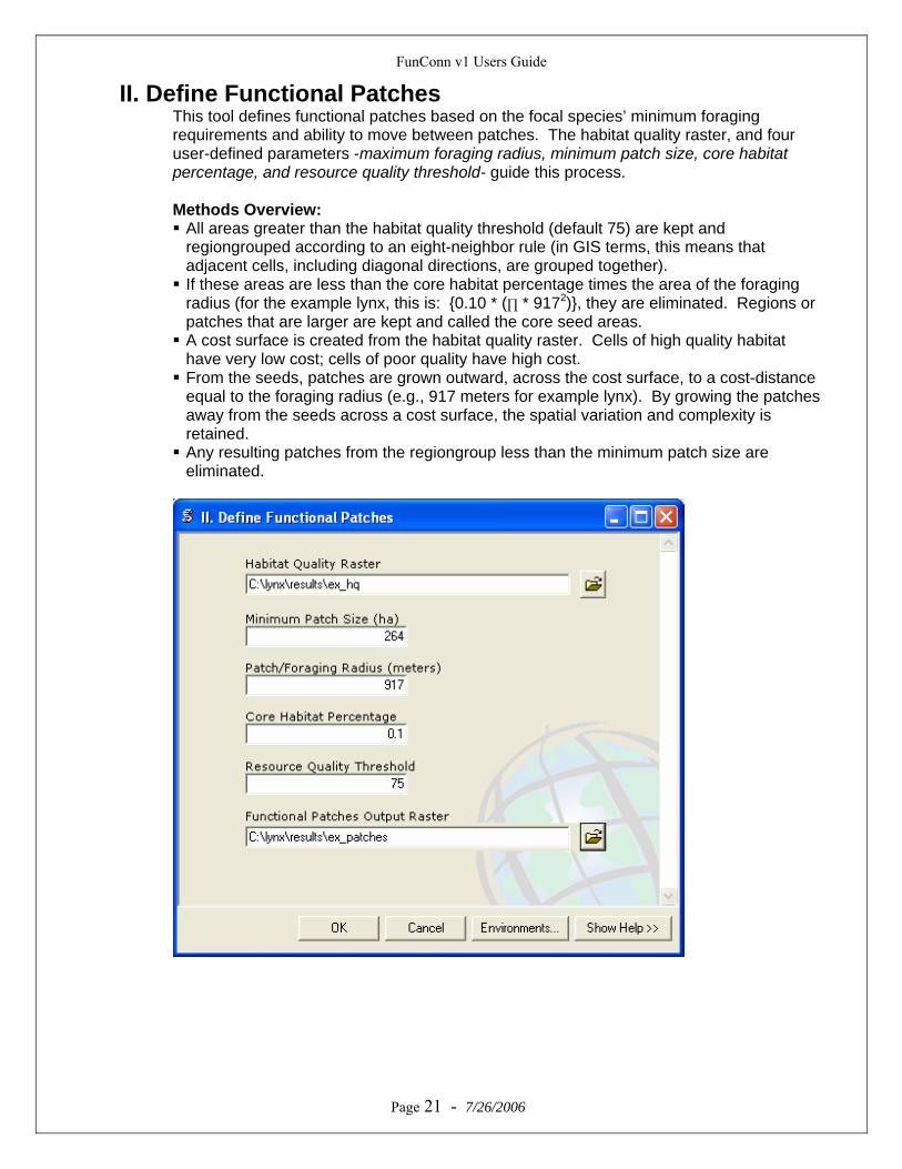
II. Define Functional Patches This tool defines functional patches based on the focal species’ minimum foraging requirements and ability to move between patches. The habitat quality raster, and four user-defined parameters -maximum foraging radius, minimum patch size, core habitat percentage, and resource quality threshold- guide this process. Methods Overview: All areas greater than the habitat quality threshold (default 75) are kept and regiongrouped according to an eight-neighbor rule (in GIS terms, this means that adjacent cells, including diagonal directions, are grouped together).

If these areas are less than the core habitat percentage times the area of the foraging radius (for the example lynx, this is: {0.10 * (∏ * 9172)}, they are eliminated. Regions or patches that are larger are kept and called the core seed areas.

A cost surface is created from the habitat quality raster. Cells of high quality habitat have very low cost; cells of poor quality have high cost.

From the seeds, patches are grown outward, across the cost surface, to a cost-distance equal to the foraging radius (e.g., 917 meters for example lynx). By growing the patches away from the seeds across a cost surface, the spatial variation and complexity is retained.

Any resulting patches from the regiongroup less than the minimum patch size are eliminated.

Page 21 - 7/26/2006


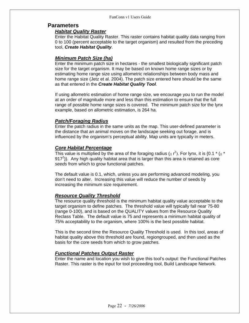
Parameters Habitat Quality Raster Enter the Habitat Quality Raster. This raster contains habitat quality data ranging from 0 to 100 (percent acceptable to the target organism) and resulted from the preceding tool, Create Habitat Quality. Minimum Patch Size (ha) Enter the minimum patch size in hectares - the smallest biologically significant patch size for the target organism. It may be based on known home range sizes or by estimating home range size using allometric relationships between body mass and home range size (Jetz et al. 2004). The patch size entered here should be the same as that entered in the Create Habitat Quality Tool. If using allometric estimation of home range size, we encourage you to run the model at an order of magnitude more and less than this estimation to ensure that the full range of possible home range sizes is covered. The minimum patch size for the lynx example, based on allometric estimation, is 264 ha. Patch/Foraging Radius Enter the patch radius in the same units as the map. This user-defined parameter is the distance that an animal moves on the landscape seeking out forage, and is influenced by the organism’s perceptual ability. Map units are typically in meters. Core Habitat Percentage This value is multiplied by the area of the foraging radius (∏ r2). For lynx, it is {0.1 * (∏ * 9172)}. Any high quality habitat area that is larger than this area is retained as core seeds from which to grow functional patches. The default value is 0.1, which, unless you are performing advanced modeling, you don’t need to alter. Increasing this value will reduce the number of seeds by increasing the minimum size requirement. Resource Quality Threshold The resource quality threshold is the minimum habitat quality value acceptable to the target organism to define patches. The threshold value will typically fall near 75-80 (range 0-100), and is based on the QUALITY values from the Resource Quality Reclass Table. The default value is 75 and represents a minimum habitat quality of 75% acceptability to the organism, where 100% is the best possible habitat. This is the second time the Resource Quality Threshold is used. In this tool, areas of habitat quality above this threshold are found, regiongrouped, and then used as the basis for the core seeds from which to grow patches. Functional Patches Output Raster Enter the name and location you wish to give this tool’s output: the Functional Patches Raster. This raster is the input for tool proceeding tool, Build Landscape Network.

Page 22 - 7/26/2006

!

!

!

!

!

!

!

!

!

!

!

!

!

!

!

!

!

!

!

!

!

!

!

!!

!

!

!

!

!

!Vail

Como

Bond

Avon

Alma

McCoy

Grant

Eagle

Burns

Aspen

Kokomo

Gilman

Frisco

Fraser

Empire

Dillon

Climax

Wolcott

Minturn

Edwards

Redcliff

Meredith

Fairplay

Montezuma

Leadville

Jefferson

Georgetown

Woody Creek


Breckenridge

Example Lynx Functional Patches: Vail Pass, Colorado

ª

Vail Pass

0 5 10 15 202.5Miles

§̈¦I-70

Legendhighways

patches=uniquecolors

*dark areas in the center of the patches are high quality "core" areas; small black areas outside of the patches are high quality but not large enough to be viable patches.


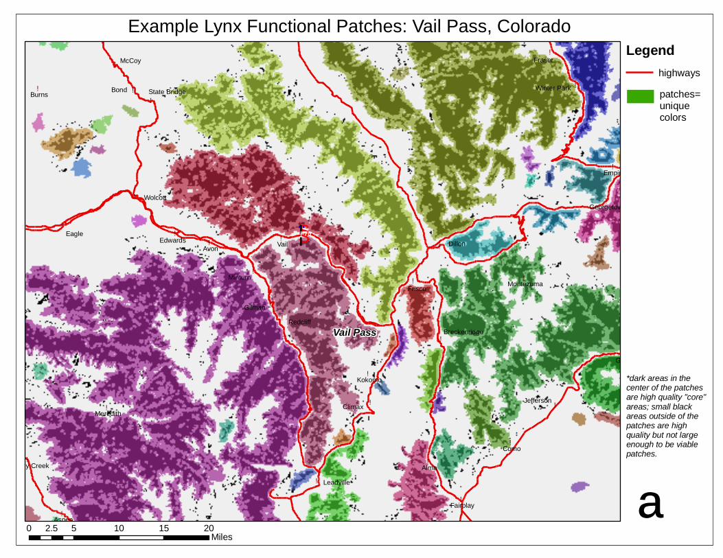
III. Build Landscape Network The Build Landscape Network Tool creates a landscape network representing habitat patch connectivity. This is accomplished by using functional habitat patches as source regions and land cover data as a movement resistance surface. The landscape network is comprised of nodes, patches, edges, linkages, corridors, and relationship tables. Methods Overview: The land cover with disturbance raster is reclassified according to user-defined permeability values found in the permeability reclass table. This raster is multiplied by an optional permeability raster (e.g., slope-perm) and then inverted to create a cost surface for the study area.

Allocation zones are grown away from the source patches across the cost surface until they meet.

The meeting point of the allocation zones are called allocation boundaries. These boundaries are 2-cells wide and are comprised of a distribution of cost-distance values.

Depending on the user-specified qn value, a certain percentage of the cell groups are extracted and serve as mid-points for a set of initial linkages between patches.

The initial linkages are joined from each qn cell group to the nearest point on the source patch.

A second set of allocation zones are grown outward from the initial linkages; where they meet are considered fences and are removed from each allocation zone so that unique corridors cannot merge between patches.

Within each new allocation zone, the cells less than the specified qn value are pulled out to form the corridors.

The least-cost cell at the mid-point and patch boundary of each corridor is found to create the refined linkages.

Multiple-edges are formed between each pair by using the same mid-point as the linkage. The edges are then formed by straight line segments from patch centroid to midpoint to patch centroid.

Page 24 - 7/26/2006


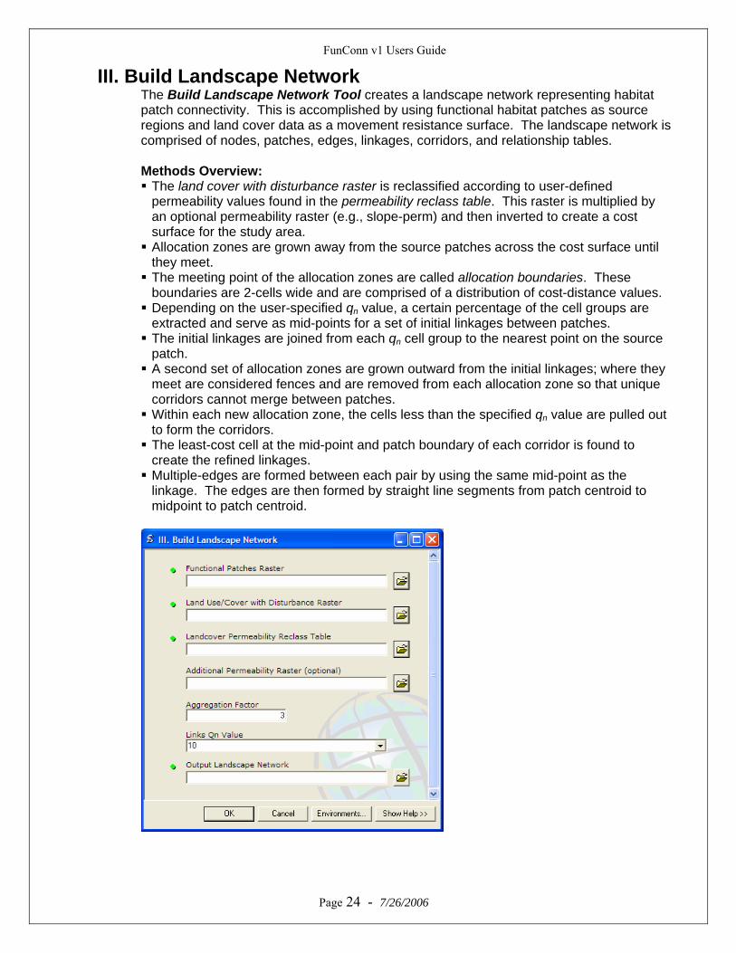
Parameters Functional Patches Raster Patches can either be the output from the preceding tool, Define Functional Patches, or an integer raster with unique patches generated by the user. Land Cover with Disturbance Raster This must be a categorical raster dataset that contains natural land cover and features that represent disturbances to the target organism such as roads, urban areas, agricultural areas, etc. This raster can be USGS NLCD, USGS GAP, or user-defined, with disturbances such as roads (e.g., by road type or traffic volume) burned into it. The example raster is c:\lynx\vp_disturb. The raster is the same as used in the Create Habitat Quality Tool.

Land Cover Permeability Reclass Table This table reclassifies the land cover with disturbance raster based on how easily an organism can move through a given class. This is not the same as habitat quality. For example, a land cover class might have a very low habitat quality value but still is highly permeable. In the case of lynx, ponderosa pine woodland does not offer valuable foraging or denning habitat but does provide excellent visibility and escape cover, so is readily moved through. Keep in mind that permeability is the inverse of resistance. Permeability is multiplied by the additional permeability raster (optional) and then inverted to generate the cost weight surface of resistance values. Format:


1. VALUE- short or long integer, 0 decimal places; unique class values for each land cover type.

2. PERMVALUE- short or long integer, 6 decimal places, ranging from 0.000000 – 1.000000; permeability value for each unique land cover class.

Example Table:

The example table is c:\lynx\permeability.dbf (Table 5).

Table 5. Example lynx permeability classes from c:\lynx\vp_perm.

Page 25 - 7/26/2006

VALUE DEFINITION PERMVALUE 22 Rocky Mountain Aspen Forest and Woodland 1.000000

32 Rocky Mountain Montane Mesic Mixed Conifer Forest and Woodland 1.000000

41 Rocky Mountain Gambel Oak-Mixed Montane Shrubland 0.800000

68 Chihuahuan Gypsophilous Grassland and Steppe 0.200000

83 North American Warm Desert Riparian Woodland and Shrubland 0.100000

7 Western Great Plains Cliff and Outcrop 0.100000

17 North American Warm Desert Active and Stabilized Dune 0.100000

28 Rocky Mountain Subalpine Mesic Spruce-Fir Forest and Woodland 1.000000

90005 Developed, Medium - High Intensity, Class 112 in the swrgp_funconn 0.005000


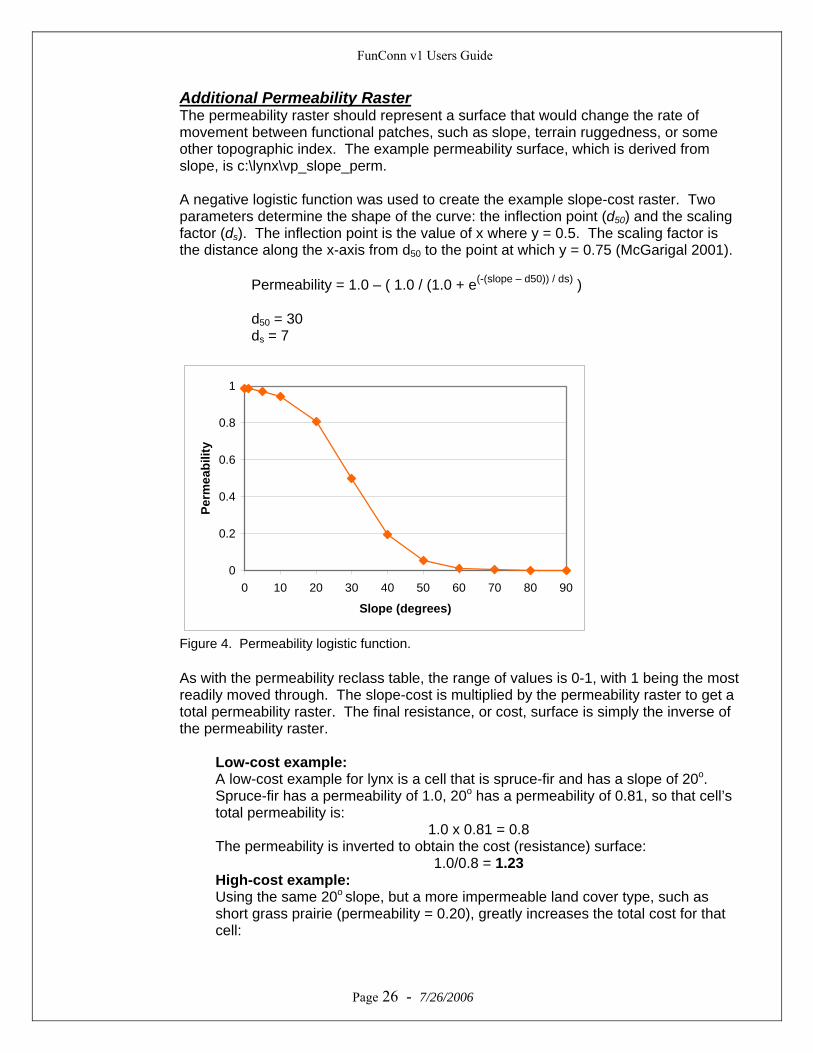
Additional Permeability Raster The permeability raster should represent a surface that would change the rate of movement between functional patches, such as slope, terrain ruggedness, or some other topographic index. The example permeability surface, which is derived from slope, is c:\lynx\vp_slope_perm. A negative logistic function was used to create the example slope-cost raster. Two parameters determine the shape of the curve: the inflection point (d50) and the scaling factor (ds). The inflection point is the value of x where y = 0.5. The scaling factor is the distance along the x-axis from d50 to the point at which y = 0.75 (McGarigal 2001).

Permeability = 1.0 – ( 1.0 / (1.0 + e(-(slope – d50)) / ds) )

d50 = 30 ds = 7

0

0.2

0.4

0.6

0.8

1

0 10 20 30 40 50 60 70 80 90

Slope (degrees)

Perm

eabi

lity

Figure 4. Permeability logistic function. As with the permeability reclass table, the range of values is 0-1, with 1 being the most readily moved through. The slope-cost is multiplied by the permeability raster to get a total permeability raster. The final resistance, or cost, surface is simply the inverse of the permeability raster.

Low-cost example: A low-cost example for lynx is a cell that is spruce-fir and has a slope of 20o. Spruce-fir has a permeability of 1.0, 20o has a permeability of 0.81, so that cell’s total permeability is:

1.0 x 0.81 = 0.8 The permeability is inverted to obtain the cost (resistance) surface:

1.0/0.8 = 1.23 High-cost example:

Page 26 - 7/26/2006

Using the same 20o slope, but a more impermeable land cover type, such as short grass prairie (permeability = 0.20), greatly increases the total cost for that cell:


Total permeability: 0.81 x 0.2 = 0.162 Cost-weight (resistance): 1.0/0.162 = 6.17

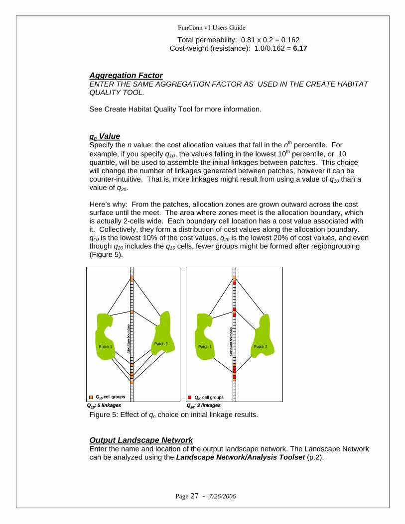
Aggregation Factor ENTER THE SAME AGGREGATION FACTOR AS USED IN THE CREATE HABITAT QUALITY TOOL. See Create Habitat Quality Tool for more information. qn Value Specify the n value: the cost allocation values that fall in the nth percentile. For example, if you specify q10, the values falling in the lowest 10th percentile, or .10 quantile, will be used to assemble the initial linkages between patches. This choice will change the number of linkages generated between patches, however it can be counter-intuitive. That is, more linkages might result from using a value of q10 than a value of q20. Here’s why: From the patches, allocation zones are grown outward across the cost surface until the meet. The area where zones meet is the allocation boundary, which is actually 2-cells wide. Each boundary cell location has a cost value associated with it. Collectively, they form a distribution of cost values along the allocation boundary. q10 is the lowest 10% of the cost values, q20 is the lowest 20% of cost values, and even though q20 includes the q10 cells, fewer groups might be formed after regiongrouping (Figure 5).

Q10 cell groups Q20 cell groups

Q10: 5 linkages Q20: 3 linkages

allo

catio

n bo

unda

ry

allo

catio

n bo

unda

ry

Patch 2Patch 2Patch 1 Patch 1

Q10 cell groups Q20 cell groups

Q10: 5 linkages Q20: 3 linkages

allo

catio

n bo

unda

ry

allo

catio

n bo

unda

ry

Patch 2Patch 2Patch 1 Patch 1

Figure 5: Effect of qn choice on initial linkage results. Output Landscape Network

Page 27 - 7/26/2006

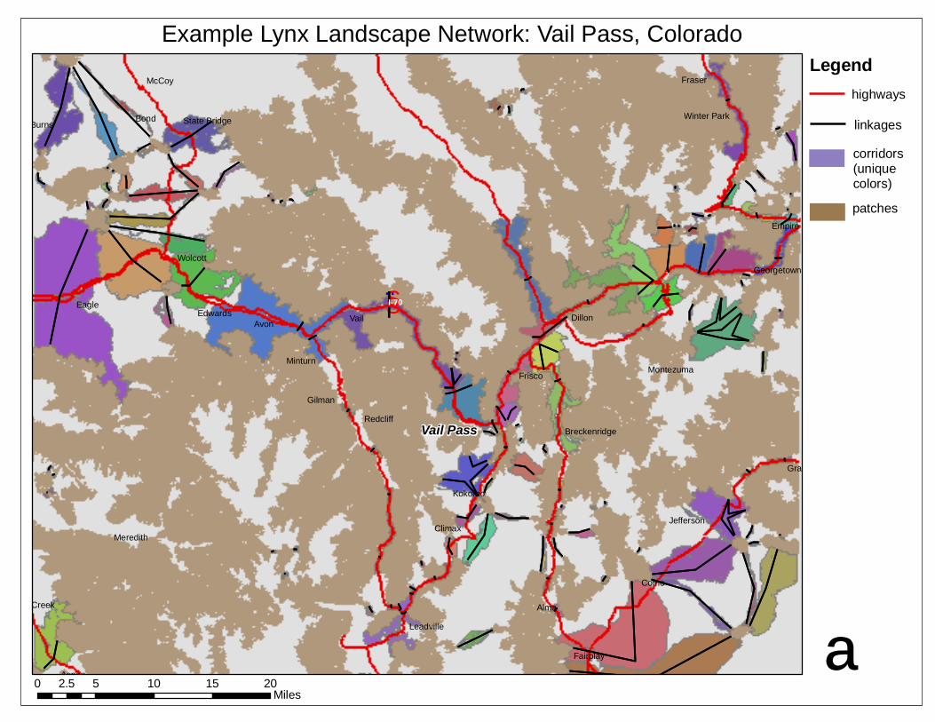
Enter the name and location of the output landscape network. The Landscape Network can be analyzed using the Landscape Network/Analysis Toolset (p.2).

Vail

Como

Bond

Avon

Alma

McCoy

Grant

Eagle

Burns

Aspen

Kokomo

Gilman

Frisco

Fraser

Empire

Dillon

Climax

Wolcott

Minturn

Edwards

Redcliff

Meredith

Fairplay

Montezuma

Leadville

Jefferson

Georgetown

Woody Creek


Breckenridge

Example Lynx Landscape Network: Vail Pass, Colorado

ª

Vail Pass

0 5 10 15 202.5Miles

§̈¦I-70

Legendhighways

corridors(unique colors)

patches

linkages


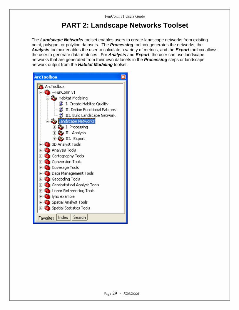
PART 2: Landscape Networks Toolset The Landscape Networks toolset enables users to create landscape networks from existing point, polygon, or polyline datasets. The Processing toolbox generates the networks, the Analysis toolbox enables the user to calculate a variety of metrics, and the Export toolbox allows the user to generate data matrices. For Analysis and Export, the user can use landscape networks that are generated from their own datasets in the Processing steps or landscape network output from the Habitat Modeling toolset.

Page 29 - 7/26/2006


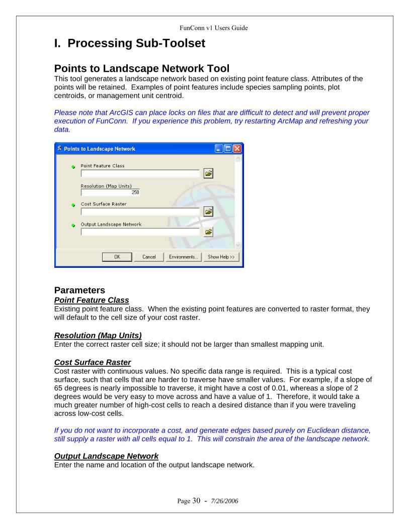
I. Processing Sub-Toolset Points to Landscape Network Tool This tool generates a landscape network based on existing point feature class. Attributes of the points will be retained. Examples of point features include species sampling points, plot centroids, or management unit centroid. Please note that ArcGIS can place locks on files that are difficult to detect and will prevent proper execution of FunConn. If you experience this problem, try restarting ArcMap and refreshing your data.

Parameters Point Feature Class Existing point feature class. When the existing point features are converted to raster format, they will default to the cell size of your cost raster. Resolution (Map Units) Enter the correct raster cell size; it should not be larger than smallest mapping unit. Cost Surface Raster Cost raster with continuous values. No specific data range is required. This is a typical cost surface, such that cells that are harder to traverse have smaller values. For example, if a slope of 65 degrees is nearly impossible to traverse, it might have a cost of 0.01, whereas a slope of 2 degrees would be very easy to move across and have a value of 1. Therefore, it would take a much greater number of high-cost cells to reach a desired distance than if you were traveling across low-cost cells. If you do not want to incorporate a cost, and generate edges based purely on Euclidean distance, still supply a raster with all cells equal to 1. This will constrain the area of the landscape network. Output Landscape Network

Page 30 - 7/26/2006

Enter the name and location of the output landscape network.


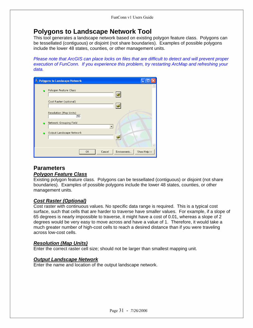
Polygons to Landscape Network Tool This tool generates a landscape network based on existing polygon feature class. Polygons can be tessellated (contiguous) or disjoint (not share boundaries). Examples of possible polygons include the lower 48 states, counties, or other management units. Please note that ArcGIS can place locks on files that are difficult to detect and will prevent proper execution of FunConn. If you experience this problem, try restarting ArcMap and refreshing your data.

Parameters Polygon Feature Class Existing polygon feature class. Polygons can be tessellated (contiguous) or disjoint (not share boundaries). Examples of possible polygons include the lower 48 states, counties, or other management units. Cost Raster (Optional) Cost raster with continuous values. No specific data range is required. This is a typical cost surface, such that cells that are harder to traverse have smaller values. For example, if a slope of 65 degrees is nearly impossible to traverse, it might have a cost of 0.01, whereas a slope of 2 degrees would be very easy to move across and have a value of 1. Therefore, it would take a much greater number of high-cost cells to reach a desired distance than if you were traveling across low-cost cells. Resolution (Map Units) Enter the correct raster cell size; should not be larger than smallest mapping unit. Output Landscape Network Enter the name and location of the output landscape network.

Page 31 - 7/26/2006


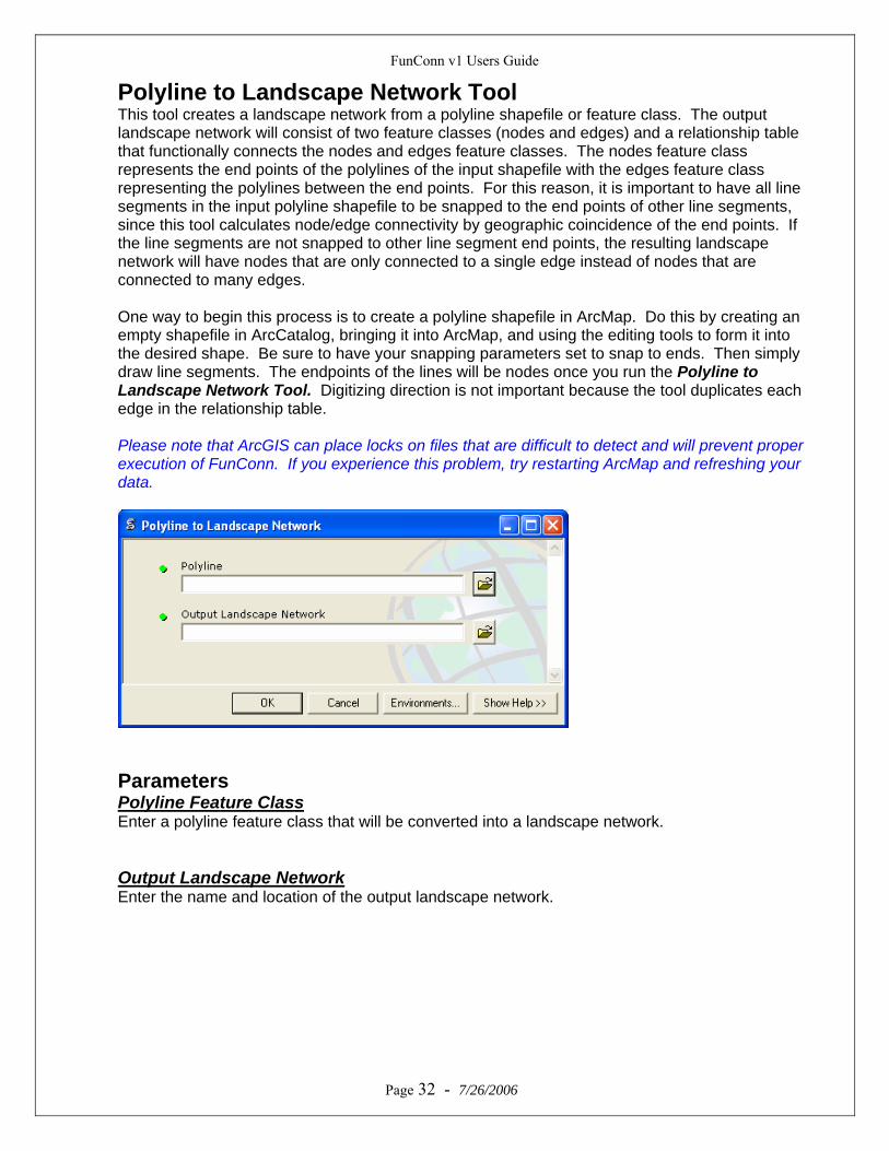
Polyline to Landscape Network Tool This tool creates a landscape network from a polyline shapefile or feature class. The output landscape network will consist of two feature classes (nodes and edges) and a relationship table that functionally connects the nodes and edges feature classes. The nodes feature class represents the end points of the polylines of the input shapefile with the edges feature class representing the polylines between the end points. For this reason, it is important to have all line segments in the input polyline shapefile to be snapped to the end points of other line segments, since this tool calculates node/edge connectivity by geographic coincidence of the end points. If the line segments are not snapped to other line segment end points, the resulting landscape network will have nodes that are only connected to a single edge instead of nodes that are connected to many edges. One way to begin this process is to create a polyline shapefile in ArcMap. Do this by creating an empty shapefile in ArcCatalog, bringing it into ArcMap, and using the editing tools to form it into the desired shape. Be sure to have your snapping parameters set to snap to ends. Then simply draw line segments. The endpoints of the lines will be nodes once you run the Polyline to Landscape Network Tool. Digitizing direction is not important because the tool duplicates each edge in the relationship table. Please note that ArcGIS can place locks on files that are difficult to detect and will prevent proper execution of FunConn. If you experience this problem, try restarting ArcMap and refreshing your data.

Parameters Polyline Feature Class Enter a polyline feature class that will be converted into a landscape network. Output Landscape Network Enter the name and location of the output landscape network.

Page 32 - 7/26/2006


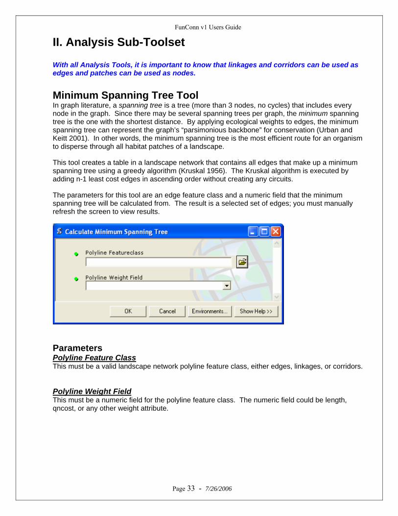
II. Analysis Sub-Toolset With all Analysis Tools, it is important to know that linkages and corridors can be used as edges and patches can be used as nodes. Minimum Spanning Tree Tool In graph literature, a spanning tree is a tree (more than 3 nodes, no cycles) that includes every node in the graph. Since there may be several spanning trees per graph, the minimum spanning tree is the one with the shortest distance. By applying ecological weights to edges, the minimum spanning tree can represent the graph’s “parsimonious backbone” for conservation (Urban and Keitt 2001). In other words, the minimum spanning tree is the most efficient route for an organism to disperse through all habitat patches of a landscape.

This tool creates a table in a landscape network that contains all edges that make up a minimum spanning tree using a greedy algorithm (Kruskal 1956). The Kruskal algorithm is executed by adding n-1 least cost edges in ascending order without creating any circuits.

The parameters for this tool are an edge feature class and a numeric field that the minimum spanning tree will be calculated from. The result is a selected set of edges; you must manually refresh the screen to view results.

Parameters Polyline Feature Class This must be a valid landscape network polyline feature class, either edges, linkages, or corridors. Polyline Weight Field This must be a numeric field for the polyline feature class. The numeric field could be length, qncost, or any other weight attribute.

Page 33 - 7/26/2006


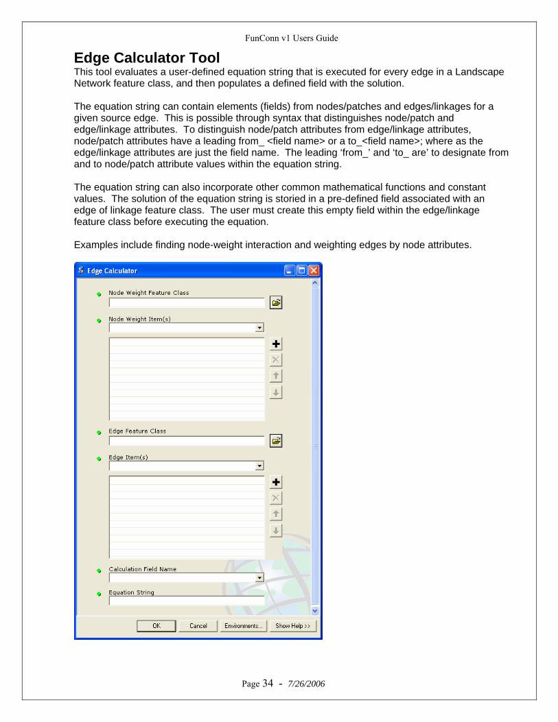
Edge Calculator Tool This tool evaluates a user-defined equation string that is executed for every edge in a Landscape Network feature class, and then populates a defined field with the solution. The equation string can contain elements (fields) from nodes/patches and edges/linkages for a given source edge. This is possible through syntax that distinguishes node/patch and edge/linkage attributes. To distinguish node/patch attributes from edge/linkage attributes, node/patch attributes have a leading from_ <field name> or a to_<field name>; where as the edge/linkage attributes are just the field name. The leading ‘from_’ and ‘to_ are’ to designate from and to node/patch attribute values within the equation string. The equation string can also incorporate other common mathematical functions and constant values. The solution of the equation string is storied in a pre-defined field associated with an edge of linkage feature class. The user must create this empty field within the edge/linkage feature class before executing the equation. Examples include finding node-weight interaction and weighting edges by node attributes.

Page 34 - 7/26/2006


Parameters Node Feature Class Select a landscape network point or polygon feature class. This could be nodes or patches. Node Weight Item(s) Numeric field(s) of the point or polygon feature class that will be referenced in the equation string. Edge Feature Class This is a valid landscape network polyline feature class; use linkages, edges, or corridors. Edge Item(s) Numeric field(s) of the polyline feature class that will be referenced in the equation string Calculation Field Name Field associated with the edges/linkages feature class that will hold equation string solution. This field must be created by the user prior to running the script. Equation String DO NOT ADD SPACES ANYWHERE IN EQUATION STRING. Network Functions:

Fields associated with Nodes or Patches must have a leading from_<field name> or a to_<field name> (e.g., (from_Shape_Area*to_Shape_Area) /ShapeLength)

Mathematical functions such as pow(x,y) can be entered as

pow(from_Shape_Area,2). This signifies that the area Shape_Area of the from node is going to be set to the power of two.

Available Mathematical Functions:

The syntax of the mathematical functions is as follows, x and y should be replaced with feature class field names or constant values.

+, -, *, / exp(x) log(x) log10(x) pow(x,y) sin(x) sqrt(x) tan(x) () operation separators

Example equation strings:

The average patch area divided by edge/linkage/corridor length: ((from_Shape_Area+to_Shape_Area)/2)/Shape_Length

The area of the to Patch multiplied by the Edge length: (to_Shape_Area*Shape_length)

Page 35 - 7/26/2006

Least-cost distance between nodes, Cij: pow(qncost,1.75)


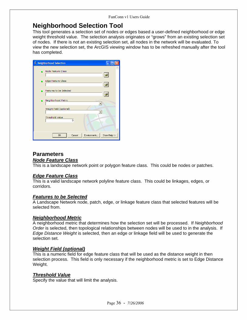
Neighborhood Selection Tool This tool generates a selection set of nodes or edges based a user-defined neighborhood or edge weight threshold value. The selection analysis originates or “grows” from an existing selection set of nodes. If there is not an existing selection set, all nodes in the network will be evaluated. To view the new selection set, the ArcGIS viewing window has to be refreshed manually after the tool has completed.

Parameters Node Feature Class This is a landscape network point or polygon feature class. This could be nodes or patches. Edge Feature Class This is a valid landscape network polyline feature class. This could be linkages, edges, or corridors. Features to be Selected A Landscape Network node, patch, edge, or linkage feature class that selected features will be selected from. Neighborhood Metric A neighborhood metric that determines how the selection set will be processed. If Neighborhood Order is selected, then topological relationships between nodes will be used to in the analysis. If Edge Distance Weight is selected, then an edge or linkage field will be used to generate the selection set. Weight Field (optional) This is a numeric field for edge feature class that will be used as the distance weight in then selection process. This field is only necessary if the neighborhood metric is set to Edge Distance Weight. Threshold Value

Page 36 - 7/26/2006

Specify the value that will limit the analysis.


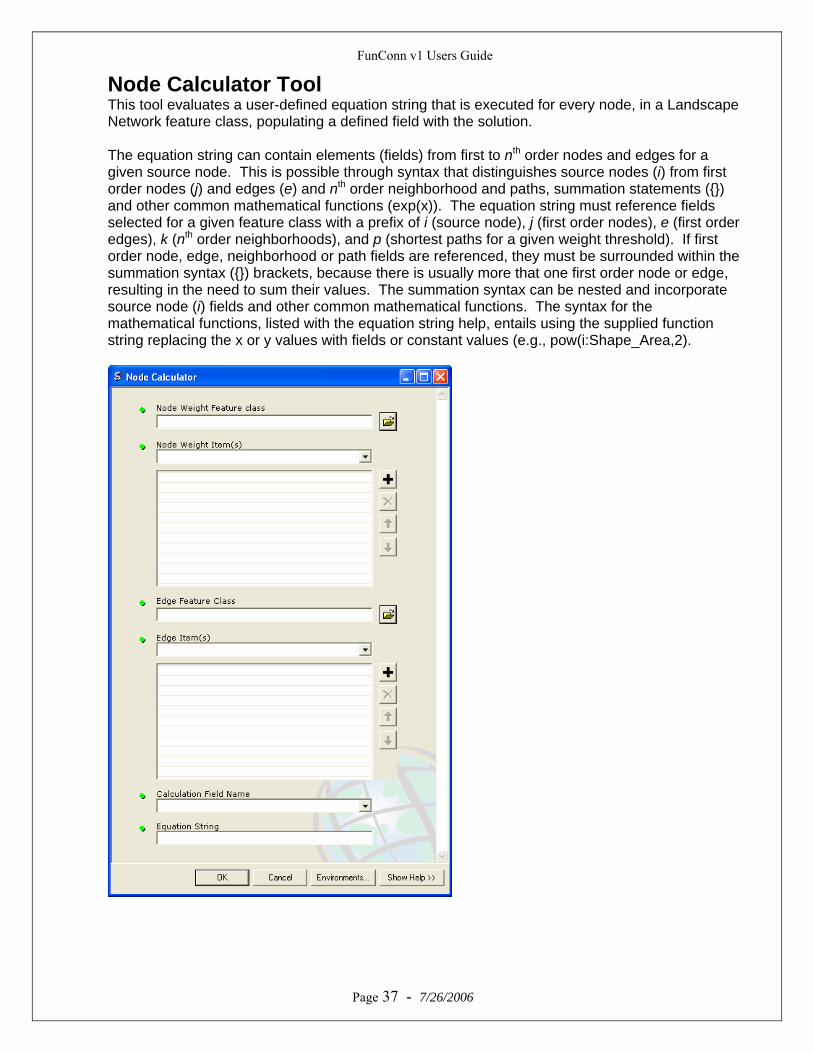
Node Calculator Tool This tool evaluates a user-defined equation string that is executed for every node, in a Landscape Network feature class, populating a defined field with the solution. The equation string can contain elements (fields) from first to nth order nodes and edges for a given source node. This is possible through syntax that distinguishes source nodes (i) from first order nodes (j) and edges (e) and nth order neighborhood and paths, summation statements ({}) and other common mathematical functions (exp(x)). The equation string must reference fields selected for a given feature class with a prefix of i (source node), j (first order nodes), e (first order edges), k (nth order neighborhoods), and p (shortest paths for a given weight threshold). If first order node, edge, neighborhood or path fields are referenced, they must be surrounded within the summation syntax ({}) brackets, because there is usually more that one first order node or edge, resulting in the need to sum their values. The summation syntax can be nested and incorporate source node (i) fields and other common mathematical functions. The syntax for the mathematical functions, listed with the equation string help, entails using the supplied function string replacing the x or y values with fields or constant values (e.g., pow(i:Shape_Area,2).

Page 37 - 7/26/2006


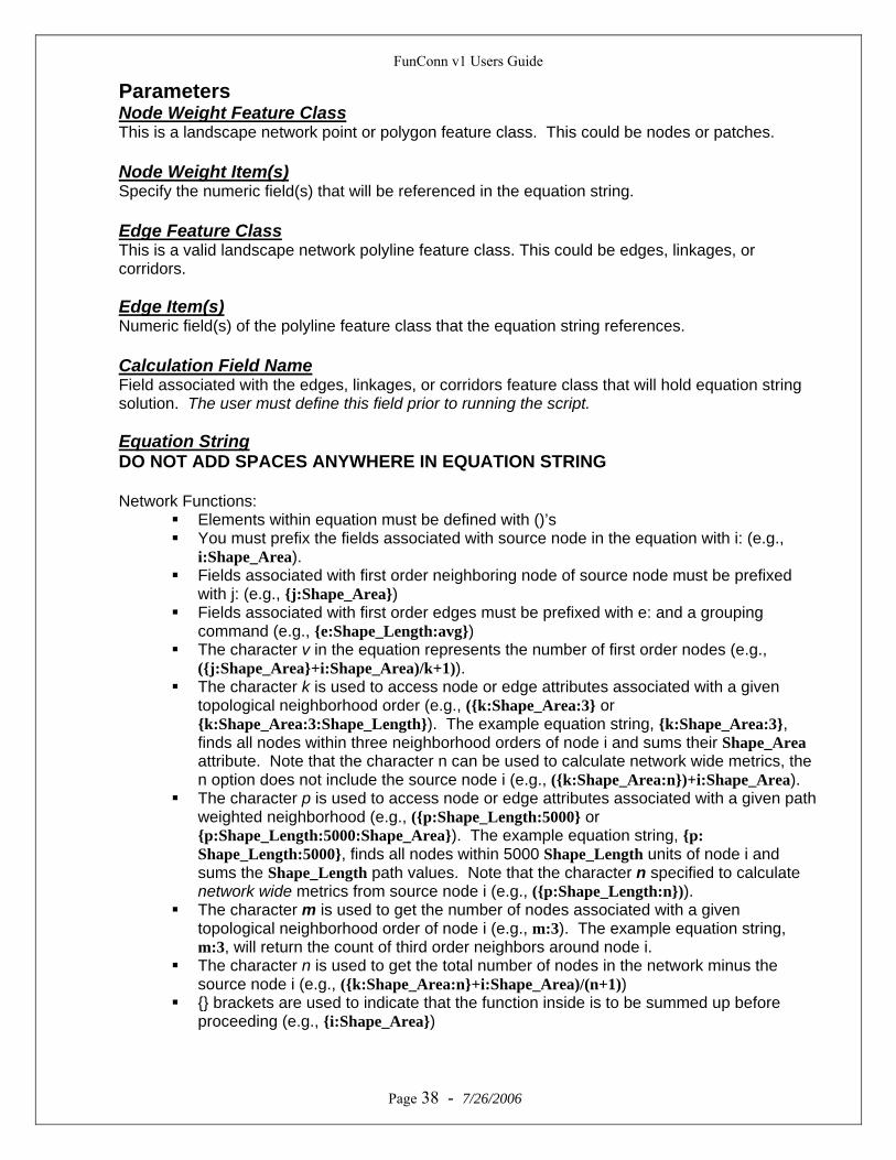
Parameters Node Weight Feature Class This is a landscape network point or polygon feature class. This could be nodes or patches. Node Weight Item(s) Specify the numeric field(s) that will be referenced in the equation string. Edge Feature Class This is a valid landscape network polyline feature class. This could be edges, linkages, or corridors. Edge Item(s) Numeric field(s) of the polyline feature class that the equation string references. Calculation Field Name Field associated with the edges, linkages, or corridors feature class that will hold equation string solution. The user must define this field prior to running the script. Equation String DO NOT ADD SPACES ANYWHERE IN EQUATION STRING Network Functions:

Elements within equation must be defined with ()’s You must prefix the fields associated with source node in the equation with i: (e.g.,

i:Shape_Area). Fields associated with first order neighboring node of source node must be prefixed

with j: (e.g., {j:Shape_Area}) Fields associated with first order edges must be prefixed with e: and a grouping

command (e.g., {e:Shape_Length:avg}) The character v in the equation represents the number of first order nodes (e.g.,

({j:Shape_Area}+i:Shape_Area)/k+1)). The character k is used to access node or edge attributes associated with a given

topological neighborhood order (e.g., ({k:Shape_Area:3} or {k:Shape_Area:3:Shape_Length}). The example equation string, {k:Shape_Area:3}, finds all nodes within three neighborhood orders of node i and sums their Shape_Area attribute. Note that the character n can be used to calculate network wide metrics, the n option does not include the source node i (e.g., ({k:Shape_Area:n})+i:Shape_Area).

The character p is used to access node or edge attributes associated with a given path weighted neighborhood (e.g., ({p:Shape_Length:5000} or {p:Shape_Length:5000:Shape_Area}). The example equation string, {p: Shape_Length:5000}, finds all nodes within 5000 Shape_Length units of node i and sums the Shape_Length path values. Note that the character n specified to calculate network wide metrics from source node i (e.g., ({p:Shape_Length:n})).

The character m is used to get the number of nodes associated with a given topological neighborhood order of node i (e.g., m:3). The example equation string, m:3, will return the count of third order neighbors around node i.

The character n is used to get the total number of nodes in the network minus the source node i (e.g., ({k:Shape_Area:n}+i:Shape_Area)/(n+1))

Page 38 - 7/26/2006

{} brackets are used to indicate that the function inside is to be summed up before proceeding (e.g., {i:Shape_Area})


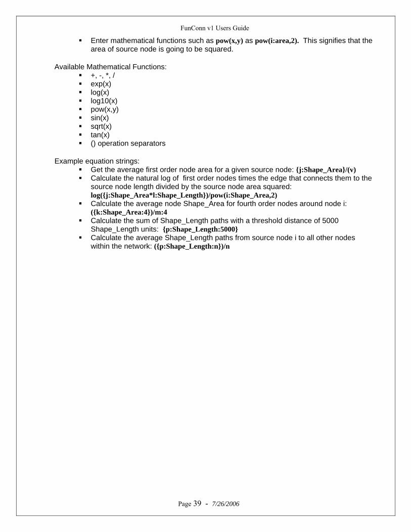
Enter mathematical functions such as pow(x,y) as pow(i:area,2). This signifies that the area of source node is going to be squared.

Available Mathematical Functions:

+, -, *, / exp(x) log(x) log10(x) pow(x,y) sin(x) sqrt(x) tan(x) () operation separators

Example equation strings:

Get the average first order node area for a given source node: {j:Shape_Area}/(v) Calculate the natural log of first order nodes times the edge that connects them to the

source node length divided by the source node area squared: log({j:Shape_Area*l:Shape_Length})/pow(i:Shape_Area,2)

Calculate the average node Shape_Area for fourth order nodes around node i: ({k:Shape_Area:4})/m:4

Calculate the sum of Shape_Length paths with a threshold distance of 5000 Shape_Length units: {p:Shape_Length:5000}

Calculate the average Shape_Length paths from source node i to all other nodes within the network: ({p:Shape_Length:n})/n

Page 39 - 7/26/2006


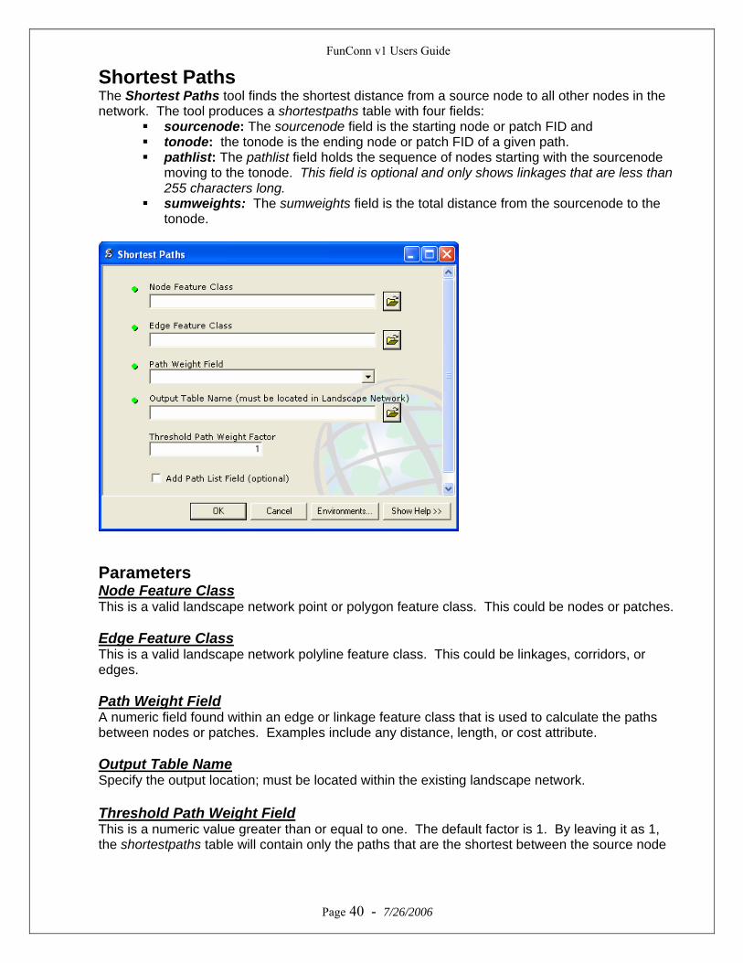
Shortest Paths The Shortest Paths tool finds the shortest distance from a source node to all other nodes in the network. The tool produces a shortestpaths table with four fields:

sourcenode: The sourcenode field is the starting node or patch FID and tonode: the tonode is the ending node or patch FID of a given path. pathlist: The pathlist field holds the sequence of nodes starting with the sourcenode

moving to the tonode. This field is optional and only shows linkages that are less than 255 characters long.

sumweights: The sumweights field is the total distance from the sourcenode to the tonode.

Parameters Node Feature Class This is a valid landscape network point or polygon feature class. This could be nodes or patches. Edge Feature Class This is a valid landscape network polyline feature class. This could be linkages, corridors, or edges. Path Weight Field A numeric field found within an edge or linkage feature class that is used to calculate the paths between nodes or patches. Examples include any distance, length, or cost attribute. Output Table Name Specify the output location; must be located within the existing landscape network. Threshold Path Weight Field

Page 40 - 7/26/2006

This is a numeric value greater than or equal to one. The default factor is 1. By leaving it as 1, the shortestpaths table will contain only the paths that are the shortest between the source node


and all other nodes. If you choose to increase this to say 1.1, then all paths from a source node to each other node that are the length of the shortest path plus 10% of that distance are included in the table. For example, if the shortest path from node A to node D was ABD and equal to a distance of 10, that is the only path between A and D the table would return (using a default threshold factor of 1). However, if a threshold factor of 1.5 is used, than any path with a distance equal to or less than 15 would also be included in the table. So then, if path ACD = 13, and path ABCD = 15, they would also both be included in the table. Therefore, for the node pair AD, the table will contain 3 paths instead of just the shortest. Be aware that increasing the Threshold Path Weight Factor will drastically increase your computing time. Add Path List Field (optional) This optional field allows from the node or patch FID’s that fall along a given path to be recorded in the field Path List. If the path exceeds 255 characters, the full linkage path will not be fully recorded.

Page 41 - 7/26/2006


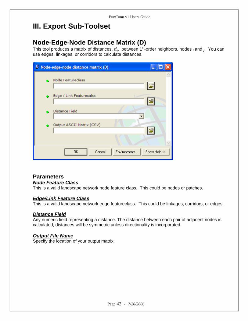
III. Export Sub-Toolset Node-Edge-Node Distance Matrix (D) This tool produces a matrix of distances, dij, between 1st-order neighbors, nodes i and j. You can use edges, linkages, or corridors to calculate distances.

Parameters Node Feature Class This is a valid landscape network node feature class. This could be nodes or patches. Edge/Link Feature Class This is a valid landscape network edge featureclass. This could be linkages, corridors, or edges. Distance Field Any numeric field representing a distance. The distance between each pair of adjacent nodes is calculated; distances will be symmetric unless directionality is incorporated. Output File NameSpecify the location of your output matrix.

Page 42 - 7/26/2006


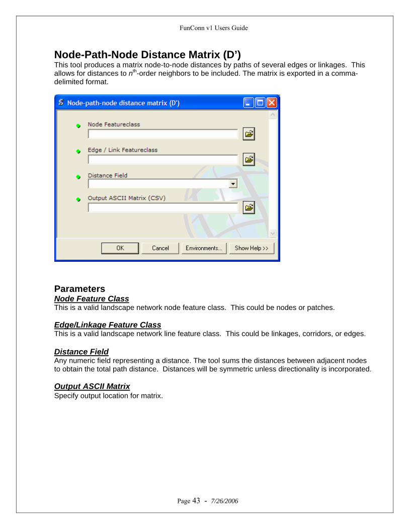
Node-Path-Node Distance Matrix (D’) This tool produces a matrix node-to-node distances by paths of several edges or linkages. This allows for distances to nth-order neighbors to be included. The matrix is exported in a comma-delimited format.

Parameters Node Feature Class This is a valid landscape network node feature class. This could be nodes or patches. Edge/Linkage Feature Class This is a valid landscape network line feature class. This could be linkages, corridors, or edges. Distance Field Any numeric field representing a distance. The tool sums the distances between adjacent nodes to obtain the total path distance. Distances will be symmetric unless directionality is incorporated. Output ASCII Matrix Specify output location for matrix.

Page 43 - 7/26/2006


References Forman, R.T.T. 2003. Road Ecology: Science and Solutions. (Island Press). Forman, R.T.T. and L.E. Alexander. 1998. Roads and their major ecological effects. Annual Review of Ecology and Systematics 29: 207- 231. Harary, F. 1969. Graph theory. Addison-Wesley, Reading, Massachusetts, USA. Jetz, W., C. Carbone, J. Fulford, and J. H. Brown. 2004. The scaling of animal space use. Science 306: 266-268. Kruskal, J. B. 1956. On the shortest spanning subtree and the traveling salesman problem. Proceedings of the American Mathematical Society 7: 48–50. McGarigal, K. 2001. CAPS documentation: Biodiversity Assessment Summary. http://www.umass.edu/landeco/research/caps/caps.html Theobald, D.M. 2006. Exploring the functional connectivity of landscapes using landscape networks. In: Conservation connectivity: Maintaining connections for nature, K.R. Crooks and M.A. Sanjayan (eds.), Cambridge University Press. Urban, D. and T. Keitt. 2001. Landscape connectivity: A graph-theoretic perspective. Ecology 82(5): 1205-121.

Page 44 - 7/26/2006

http://www.umass.edu/landeco/research/caps/caps.html


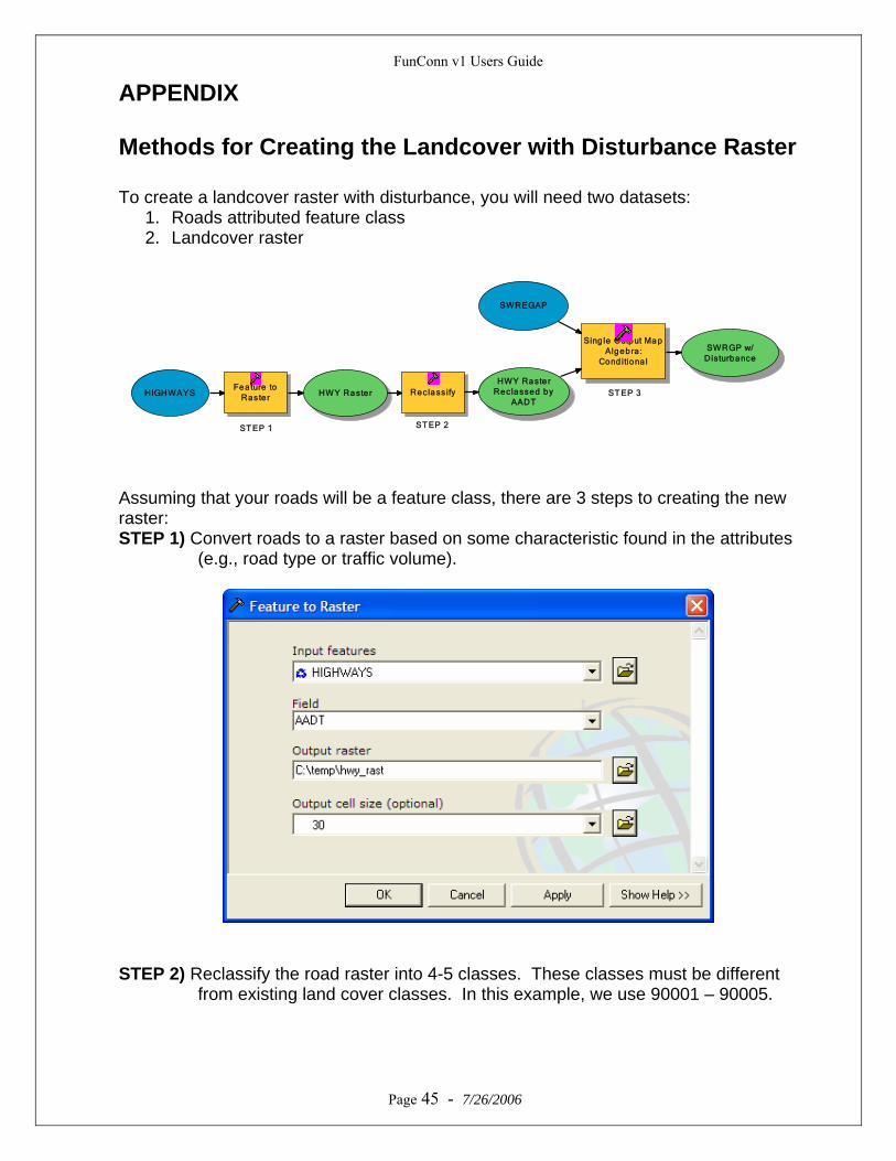
APPENDIX Methods for Creating the Landcover with Disturbance Raster To create a landcover raster with disturbance, you will need two datasets:

1. Roads attributed feature class 2. Landcover raster

HIGHWAYSFeature to

Raste r HWY Raster Reclass ifyHWY Raste r

Reclassed byAADT

Sing le Output MapAlgebra :

Cond itiona l

SWRGP w/Disturbance

SWREGAP

ST EP 1 ST EP 2

ST EP 3

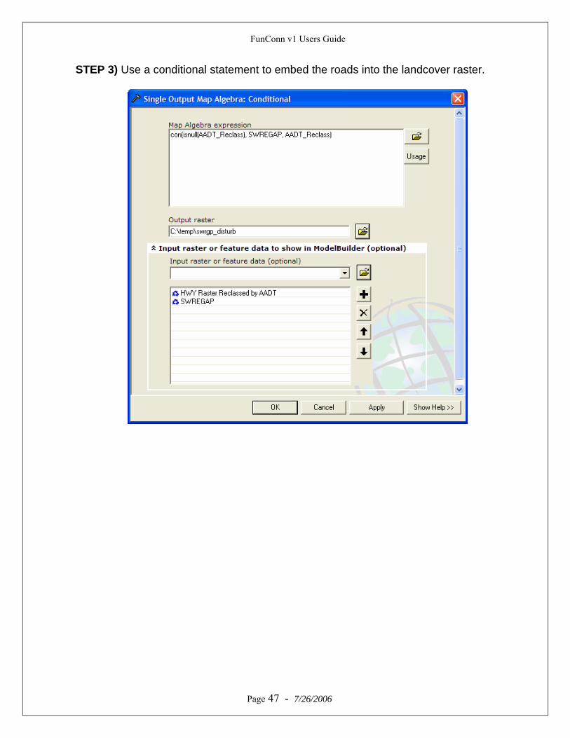
Assuming that your roads will be a feature class, there are 3 steps to creating the new raster: STEP 1) Convert roads to a raster based on some characteristic found in the attributes

(e.g., road type or traffic volume).

STEP 2) Reclassify the road raster into 4-5 classes. These classes must be different

from existing land cover classes. In this example, we use 90001 – 90005.

Page 45 - 7/26/2006


Page 46 - 7/26/2006


STEP 3) Use a conditional statement to embed the roads into the landcover raster.

Page 47 - 7/26/2006

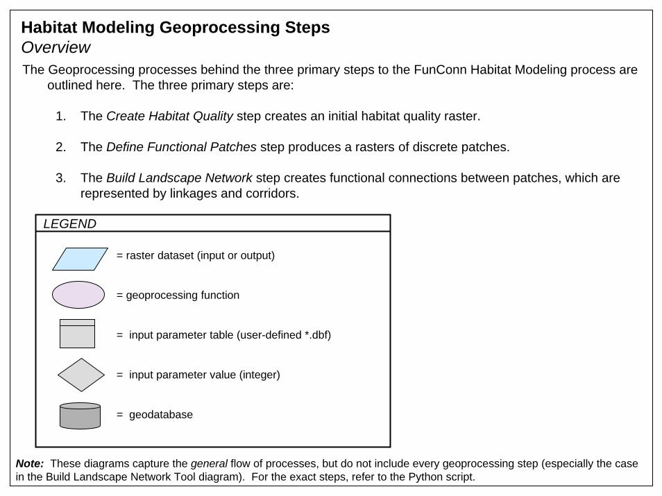
Habitat Modeling Geoprocessing StepsOverview The Geoprocessing processes behind the three primary steps to the FunConn Habitat Modeling process are

outlined here. The three primary steps are:

1. The Create Habitat Quality step creates an initial habitat quality raster.

2. The Define Functional Patches step produces a rasters of discrete patches.

3. The Build Landscape Network step creates functional connections between patches, which are represented by linkages and corridors.

= raster dataset (input or output)

= geoprocessing function

= input parameter table (user-defined *.dbf)

= input parameter value (integer)

= geodatabase

LEGEND

Note: These diagrams capture the general flow of processes, but do not include every geoprocessing step (especially the case in the Build Landscape Network Tool diagram). For the exact steps, refer to the Python script.

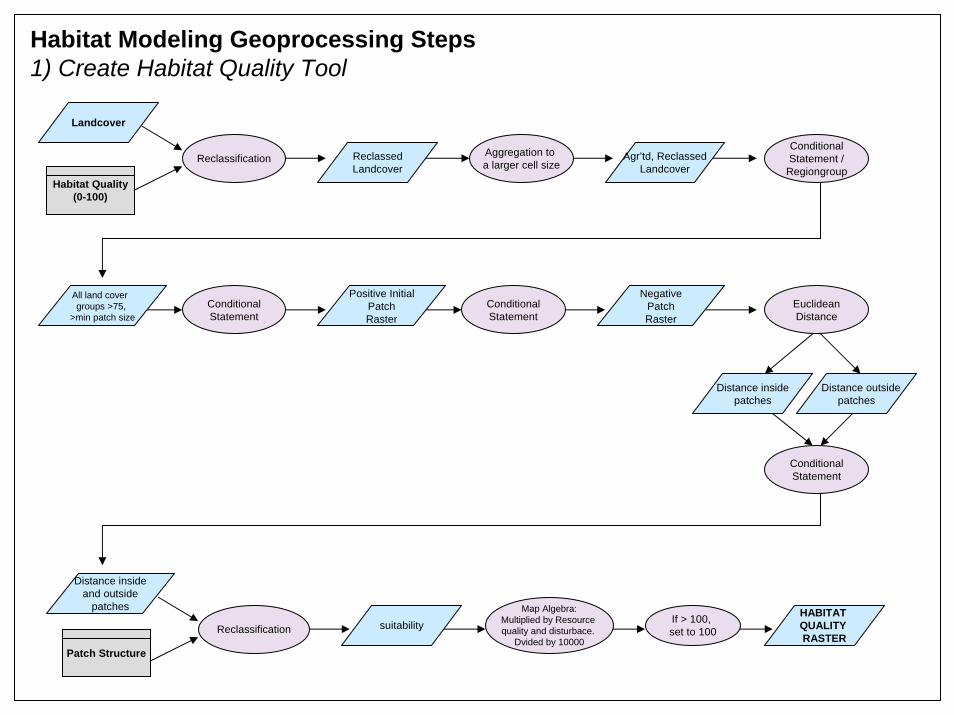
Habitat Modeling Geoprocessing Steps1) Create Habitat Quality Tool

Landcover

Reclassification

Habitat Quality(0-100)

ReclassedLandcover

Aggregation to a larger cell size

Agr’td, ReclassedLandcover

ConditionalStatement

Distance insidepatches

Reclassification suitability If > 100, set to 100

HABITAT QUALITY RASTER

Patch Structure

ConditionalStatement /

Regiongroup

All land cover groups >75,

>min patch size

Positive InitialPatchRaster


NegativePatchRaster

EuclideanDistance

Distance outsidepatches


Distance insideand outside

patches Map Algebra:Multiplied by Resource quality and disturbace.

Dvided by 10000

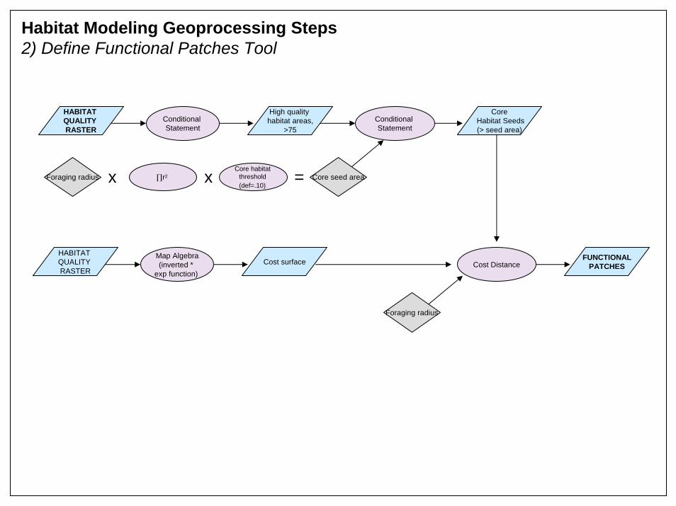
Habitat Modeling Geoprocessing Steps2) Define Functional Patches Tool

Conditional Statement

HABITAT QUALITY RASTER

∏r2Foraging radiusCore habitat

threshold (def=.10)

High quality habitat areas,

>75

Core seed area

Conditional Statement

CoreHabitat Seeds(> seed area)

x

Foraging radius

Cost DistanceHABITAT QUALITY RASTER

Map Algebra(inverted *

exp function)Cost surface FUNCTIONAL

PATCHES

x =

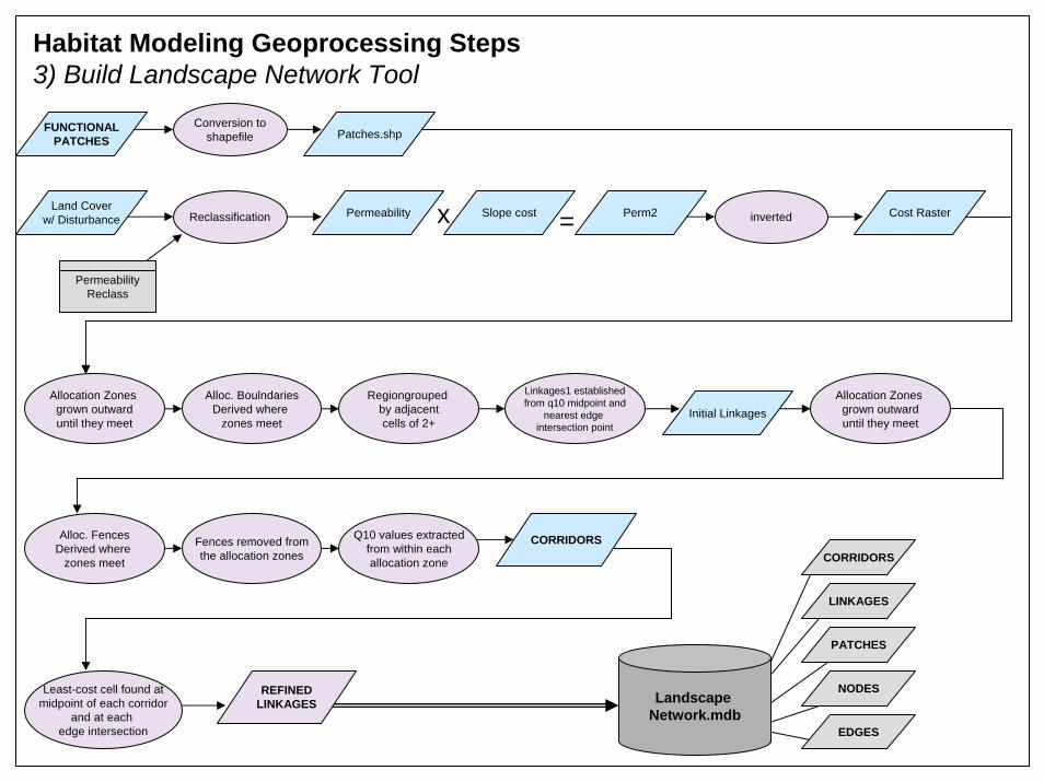
Habitat Modeling Geoprocessing Steps3) Build Landscape Network Tool

Conversion toshapefile

FUNCTIONALPATCHES Patches.shp

Reclassification

PermeabilityReclass

Permeability Slope costx invertedPerm2

Allocation Zones grown outwarduntil they meet

Alloc. BoulndariesDerived where

zones meet

Regiongrouped by adjacentcells of 2+

Linkages1 establishedfrom q10 midpoint and

nearest edge intersection point

= Cost RasterLand Coverw/ Disturbance

Initial LinkagesAllocation Zones

grown outwarduntil they meet

Alloc. FencesDerived where

zones meet

Fences removed fromthe allocation zones

Q10 values extractedfrom within eachallocation zone

CORRIDORS

Least-cost cell found atmidpoint of each corridor

and at each edge intersection

REFINEDLINKAGES Landscape

Network.mdb

CORRIDORS

LINKAGES

PATCHES

NODES

EDGES

Documents

FunConn v1 User’s Manual: ArcGIS tools for Functional ...nsu/starmap/learningmaterials/technical... · ArcGIS tools for Functional Connectivity Modeling ... FunConn v1 User’s