Embed Size (px)
Citation preview
Function Approximation
Wouter J. Den HaanLondon School of Economics
c© by Wouter J. Den Haan
Overview Polynomial approximations Splines Extra
Goal
Obtain an approximation for
f (x)
when
• f (x) is unknown, but we have some information, or• f (x) is known, but too complex to work with
Overview Polynomial approximations Splines Extra
Information available
• Either finite set of derivatives• usually at one point
• or finite set of function values• f1, · · · , fm at m nodes, x1, · · · , xm
Overview Polynomial approximations Splines Extra
Classes of approximating functions
1 polynomials
• this still gives lots of flexibility• examples of second-order polynomials
• a0 + a1x+ a2x2
• a0 + a1 ln(x) + a2 (ln (x))2
• exp(
a0 + a1 ln(x) + a2 (ln (x))2)
2 splines, e.g., linear interpolation
Overview Polynomial approximations Splines Extra
Classes of approximating functions
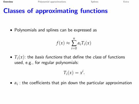
• Polynomials and splines can be expressed as
f (x) ≈n
∑i=0
αiTi(x)
• Ti(x): the basis functions that define the class of functionsused, e.g., for regular polynomials:
Ti(x) = xi.
• αi : the coeffi cients that pin down the particular approximation
Overview Polynomial approximations Splines Extra
Reducing the dimensionality
unknown f (x) : infinite dimensional object
∑ni=0 αiTi(x): n+ 1 elements
Overview Polynomial approximations Splines Extra
General procedure
• Fix the order of the approximation n• Find the coeffi cients α0, · · · , αn
• Evaluate the approximation• If necessary, increase n to get a better approximation
Overview Polynomial approximations Splines Extra
Weierstrass (sloppy definition but true)
Let f : [a, b] −→ R be any real-valued function. For large enough n,it is approximated arbitrarily well with the polynomial
n
∑i=0
αixi.
Thus, we can get an accurate approximation if
• f is not a polynomial• f is discontinuous
How can this be true?
Overview Polynomial approximations Splines Extra
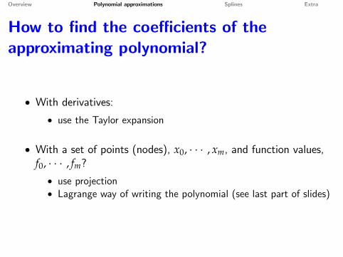
How to find the coeffi cients of theapproximating polynomial?
• With derivatives:• use the Taylor expansion
• With a set of points (nodes), x0, · · · , xm, and function values,f0, · · · , fm?• use projection• Lagrange way of writing the polynomial (see last part of slides)
Overview Polynomial approximations Splines Extra
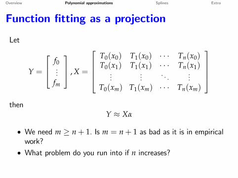
Function fitting as a projection
Let
Y =
f0...
fm
, X =
T0(x0) T1(x0) · · · Tn(x0)T0(x1) T1(x1) · · · Tn(x1)...
.... . .
...T0(xm) T1(xm) · · · Tn(xm)
then
Y ≈ Xα
• We need m ≥ n+ 1. Is m = n+ 1 as bad as it is in empiricalwork?
• What problem do you run into if n increases?
Overview Polynomial approximations Splines Extra
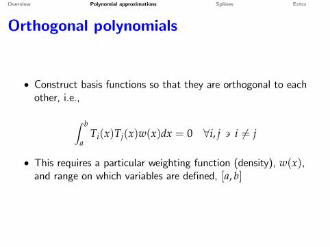
Orthogonal polynomials
• Construct basis functions so that they are orthogonal to eachother, i.e.,
∫ b
aTi(x)Tj(x)w(x)dx = 0 ∀i, j � i 6= j
• This requires a particular weighting function (density), w(x),and range on which variables are defined, [a, b]
Overview Polynomial approximations Splines Extra
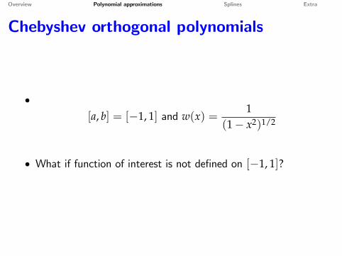
Chebyshev orthogonal polynomials
•[a, b] = [−1, 1] and w(x) =
1(1− x2)1/2
• What if function of interest is not defined on [−1, 1]?
Overview Polynomial approximations Splines Extra
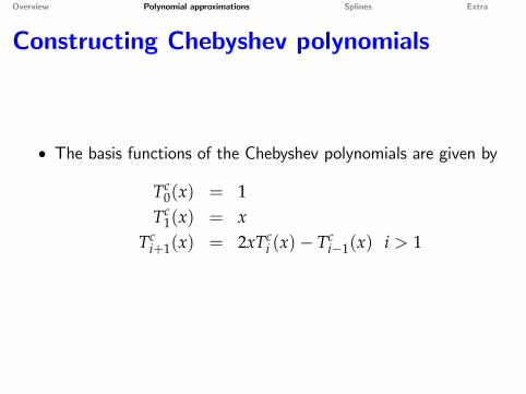
Constructing Chebyshev polynomials
• The basis functions of the Chebyshev polynomials are given by
Tc0(x) = 1
Tc1(x) = x
Tci+1(x) = 2xTc
i (x)− Tci−1(x) i > 1
Overview Polynomial approximations Splines Extra
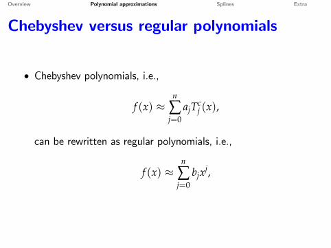
Chebyshev versus regular polynomials
• Chebyshev polynomials, i.e.,
f (x) ≈n
∑j=0
ajTcj (x),
can be rewritten as regular polynomials, i.e.,
f (x) ≈n
∑j=0
bjxj,
Overview Polynomial approximations Splines Extra
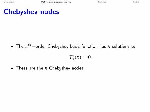
Chebyshev nodes
• The nth−order Chebyshev basis function has n solutions to
Tcn(x) = 0
• These are the n Chebyshev nodes
Overview Polynomial approximations Splines Extra
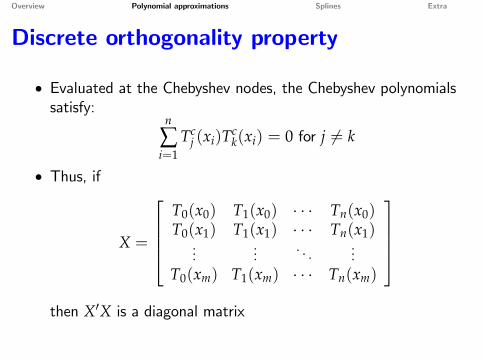
Discrete orthogonality property
• Evaluated at the Chebyshev nodes, the Chebyshev polynomialssatisfy:
n
∑i=1
Tcj (xi)Tc
k(xi) = 0 for j 6= k
• Thus, if
X =
T0(x0) T1(x0) · · · Tn(x0)T0(x1) T1(x1) · · · Tn(x1)...
.... . .
...T0(xm) T1(xm) · · · Tn(xm)
then X′X is a diagonal matrix
Overview Polynomial approximations Splines Extra
Uniform convergence
• Weierstrass =⇒ there is a good polynomial approximation
• Weierstrass ; f (x) = limn→∞ pn(x) for every sequence pn(x)
• If polynomials are fitted on Chebyshev nodes=⇒ even uniformconvergence is guaranteed
Overview Polynomial approximations Splines Extra
Splines
Inputs:
1 n+ 1 nodes, x0, · · · , xn
2 n+ 1 function values, f (x0) · · · , f (xn)
• nodes are fixed =⇒ the n+ 1 function values are thecoeffi cients of the spline
Overview Polynomial approximations Splines Extra
Piece-wise linear
• For x ∈ [xi, xi+1]
f (x) ≈(
1− x− xixi+1 − xi
)fi +
(x− xi
xi+1 − xi
)fi+1.
• That is, a separate linear function is fitted on the n intervals• Still it is easier/better to think of the coeffi cients of theapproximating function as the n+ 1 function values
Overview Polynomial approximations Splines Extra
Piece-wise linear versus polynomial
• Advantage: Shape preserving• in particular monotonicity & concavity (strict?)
• Disadvantage: not differentiable
Overview Polynomial approximations Splines Extra
Extra material
1 Lagrange interpolation
2 Higher dimensional polynomials
3 Higher-order splines
Overview Polynomial approximations Splines Extra
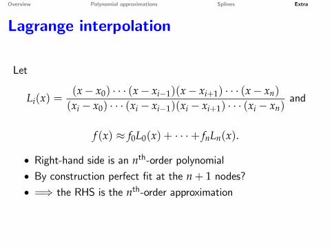
Lagrange interpolation
Let
Li(x) =(x− x0) · · · (x− xi−1)(x− xi+1) · · · (x− xn)
(xi − x0) · · · (xi − xi−1)(xi − xi+1) · · · (xi − xn)and
f (x) ≈ f0L0(x) + · · ·+ fnLn(x).
• Right-hand side is an nth-order polynomial• By construction perfect fit at the n+ 1 nodes?• =⇒ the RHS is the nth-order approximation
Overview Polynomial approximations Splines Extra
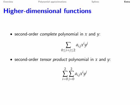
Higher-dimensional functions
• second-order complete polynomial in x and y:
∑0≤i+j≤2
ai,jxiyj
• second-order tensor product polynomial in x and y:
2
∑i=0
2
∑j=0
ai,jxiyj

Overview Polynomial approximations Splines Extra
Complete versus tensor product
• tensor product can make programming easier• simple double loop instead of condition on sum
• nth tensor has higher order term than (n+ 1)th complete• 2nd-order tensor has fourth-order power• at least locally, lower-order powers are more important=⇒ complete polynomial may be more effi cient
Overview Polynomial approximations Splines Extra
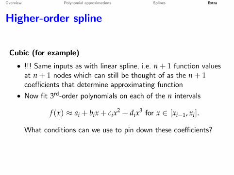
Higher-order spline
Cubic (for example)
• !!! Same inputs as with linear spline, i.e. n+ 1 function valuesat n+ 1 nodes which can still be thought of as the n+ 1coeffi cients that determine approximating function
• Now fit 3rd-order polynomials on each of the n intervals
f (x) ≈ ai + bix+ cix2 + dix3 for x ∈ [xi−1, xi].
What conditions can we use to pin down these coeffi cients?
Overview Polynomial approximations Splines Extra
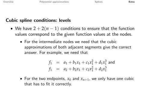
Cubic spline conditions: levels
• We have 2+ 2(n− 1) conditions to ensure that the functionvalues correspond to the given function values at the nodes.
• For the intermediate nodes we need that the cubicapproximations of both adjacent segments give the correctanswer. For example, we need that
f1 = a1 + b1x1 + c1x21 + d1x3
1 and
f1 = a2 + b2x1 + c2x21 + d2x3
1
• For the two endpoints, x0 and xn+1, we only have one cubicthat has to fit it correctly.
Overview Polynomial approximations Splines Extra
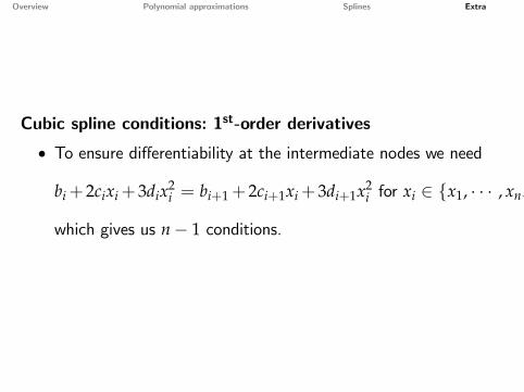
Cubic spline conditions: 1st-order derivatives
• To ensure differentiability at the intermediate nodes we need
bi+ 2cixi+ 3dix2i = bi+1+ 2ci+1xi+ 3di+1x2
i for xi ∈ {x1, · · · , xn−1},
which gives us n− 1 conditions.
Overview Polynomial approximations Splines Extra
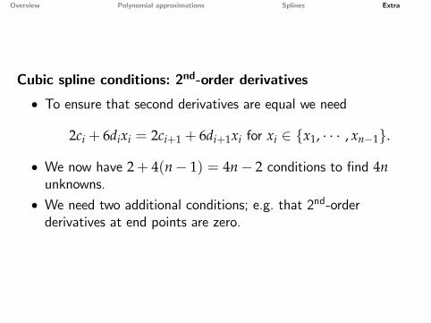
Cubic spline conditions: 2nd-order derivatives
• To ensure that second derivatives are equal we need
2ci + 6dixi = 2ci+1 + 6di+1xi for xi ∈ {x1, · · · , xn−1}.
• We now have 2+ 4(n− 1) = 4n− 2 conditions to find 4nunknowns.
• We need two additional conditions; e.g. that 2nd-orderderivatives at end points are zero.
Overview Polynomial approximations Splines Extra
Splines - additional issues
• (standard) higher-order splines do not preserve shape• higher-order diffi cult for multi-dimensional problems• first-order trivial for multi-dimensional problems
• if interval is small then nondifferentiability often doesn’t matter
Overview Polynomial approximations Splines Extra
References
• Den Haan, W.J., Numerical Integration, online lecture notes.• Heer, B., and A. Maussner, 2009, Dynamic General EquilibriumModeling.
• Judd, K. L., 1998, Numerical Methods in Economics.• Miranda, M.J, and P.L. Fackler, 2002, Applied ComputationalEconomics and Finance.