FUNCTIONAL INTEGRALS CONNECTED WITH OPERATOR EVOLUTION EQUATIONS

This article has been downloaded from IOPscience. Please scroll down to see the full text article.

1962 Russ. Math. Surv. 17 1

(http://iopscience.iop.org/0036-0279/17/5/R01)

Download details:

IP Address: 132.74.1.4

The article was downloaded on 20/08/2013 at 13:54

Please note that terms and conditions apply.

View the table of contents for this issue, or go to the journal homepage for more

Home Search Collections Journals About Contact us My IOPscience

FUNCTIONAL INTEGRALS CONNECTEDWITH OPERATOR EVOLUTION EQUATIONS

Yu.L. DALETSKII

Contents

Introduction 1

§1. The Discrete Case 4

§2. Quasi-measures and functional integrals 10

§3. Basic and generalized elements of Hubert space 24

§4. Evolution equations 39

§5. Abstract hyperbolic equations 56

§6. Fundamental solutions of evolution equations 69

§7. Functional integrals associated with abstract parabolic

equations 78

§8. The representation of generalized kernels as weak functional

integrals 98

References 105

Introduct ion

R. Feynman first used functional integrals - integrals in a functionspace - to represent solutions of differential equations. He shows in [l]that such a representation can be obtained for the solution of Schr6dinger' sequation. The method supposes that the solution ψ(*, t) of Schro'dinger'sequation

dib · ΤΓ ι /Γι Λ \

-TJ-=(WI)) (0.1)

describing the state at the point (x, t) of the phase-space is the sura ofcontributions from all "paths" along which the system could evolve fromthe initial state into the given state.

Although Feynraan' s arguments are not rigorous, they are importantheuristically. A mathematically rigorous solution on these lines was givenby M. Kac [2] in a simpler case - a classical diffusion problem.

The solution of the diffusion equation

gives the probability that the system reaches the point (x, t) from itsinitial state. The contributions of the separate paths to the solution of(0.1) are complex, whilst for (0.2) they are non-negative. Considering

1

2 Yu.L. Daletskii

them as the density of a measure on the space of paths we obtain a repre-

sentation of the solution as an integral with respect to this measure. It

turns out that the measures arising from equations with different potential

functions V(x, t) are absolutely continuous with respect to each other,

and so the solution of 0.2 can be represented as the integral of a certain

functional, defined in the space of paths, with respect to the measure

associated with the equation

the so-called Wiener measure.

This integral can be considered in two ways. We can think of it as a

Lebesgue integral with respect to the Wiener measure, or, alternatively,

as the limit of the finite sums obtained by replacing the path functions

by step-functions. As was shown by S.V. Pomin [з] for a wide class of

functionals, both approaches lead to the same result.

The equation (0.2) does not seem to be exceptional. Other second-order

equations of parabolic type have similar properties. The demonstration of

the corresponding results is the same as in the case of (0.2), and depends

on the positiveness of the fundamental solution of such equations [4].

We note that these results have an interpretation in the theory of

random processes, and the measures in the space of paths are the pro-

bability measures associated with certain Markov processes.

However, as appears from the papers of W. Feller [5] and Ε.Β. Dynkin

[б], where the structure of generating operators of Markov processes is

studied, the fundamental solutions are positive, roughly speaking, only

for second-order parabolic operators. Consequently we are not able to

construct measures similar to the Wiener measure for other evolution

equations.

There still remains the possibility of representing the solutions of

such equations as functional integrals understood as limits of finite

sums. In their survey article [7] I.M. Gel'fand and A.M. Yaglom conjec-

tured that in a certain sense functional integrals can be constructed

for a wide class of equations.

We generalize the formulation of the problem and examine the abstract

evolution equation

•§£=#(*) Ψ (0.3)

in the Hilbert space i§. We carry out an investigation in terms of the

theory of semigroups and make essential use of the properties of this

equation studied by E. Hille [в], Т. Kato [я], and Μ.A. Krasnosel' skil,

S.G. Krein, and P. Ε. Sobolevskii [io]-[l2]. It is found that (0.3) is the

abstract analogue of a parabolic equation.

In this case the fundamental solution of (0.3) is representable as a

functional integral. We introduce, at the same time, the concept of the

fundamental solution of an abstract evolution equation. In order to do

this we have to consider three spaces

where D and N are spaces of basic and generalized elements of £ [l3]-[l5],

Functional integrals connected with operator evolution equations 3

and to use the results of I.M. Gel'fand and A.G. Kostyuchenko [l5], [16]

concerning the decomposition with respect to the generalized eigen-elements

of a self-adjoint operator. These results are used in the form described

by Yu.M. Berezanskii [l7] and G.I. Kats [18].

The results obtained in this part yield a representation, as a func-

tional integral, of the solution of an equation, or of a system of equa-

tions, of parabolic type, either in the whole space or in some domain where

boundary conditions are imposed. We may then employ certain inequalities

obtained by O.A. Ladyzhenskaya [l9], [20], O.V. Guseva [2l], and

M. Schechter [22].

We consider, in particular, the case where the functional integral can

be understood as a Lebesgue integral and obtain some results concerning

the differentiation of one measure with respect to another, previously

obtained by Yu.V. Prokhorov [23] and A.V. Skorokhod [24] by the theory of

random processes. In some cases similar results are also obtained for

systems of equations.

The results described here were announced in [25]- [27].

We also consider abstract equations similar to Schr6dinger equations

and to hyperbolic systems of first order equations. The fundamental solu-

tions of such equations turn out to be generalized elements.

For abstract hyperbolic equations we are able to introduce a notion

analogous to that of characteristics. The fundamental solutions are here

representable as functional integrals understood in a generalized sense.

The contributions from separate paths are generalized functions, where

non-zero contributions arise only from paths that are everywhere

characteristic.

In the part concerning the Schr8dinger equation it was assumed that

we can associate with the equation

a measure in the functional space which, although not positive, is ofbounded variation, that we can construct a Lebesgue-Stieltjes integralwith respect to this measure, and then, passing to the limit, as ε -· 0,obtain the integral associated with the SchrOdinger equation. The factthat a similar measure is not of bounded variation was noted by theauthor [27] and R.H. Cameron [28].

Cameron demonstrated the existence of continuous integrals withrespect to the "measure" associated with Schredinger's equation

-~ = ί#ψ for analytic functionals satisfying certain conditions of growth.

He reduces the integrals to integrals with respect to the Wiener measure

by means of a change of variables and an analytic continuation.

An abstract equation

^ (0.4)

is examined - where Я is a self-adjoint operator - and is studied in twoways. In the first, [26], [27], the equation is transformed by the sub-stitution of i + ε for i, when the results for the parabolic case becomeapplicable, and we then let ε - 0 in the functional integrals so obtained.

4 Yu.L. Daletskii

In the second, [29], functional integrals can be constructed immediately

for (0.4), (as weak limits of finite sums of generalized functions).

Results similar to those valid for Schr6dinger's eauation - the simplest

case - are obtained for equations containing terms corresponding to

electro-magnetic forces, for example, Pauli's equation.

The paper begins with an examination of the discrete case motivated by

heuristic arguments. In §2 the notions of quasi-measure and functional

integral are introduced and their simplest properties are studied. In §3

the spaces of basic and generalized elements are described. In §§4,5,6

the properties of evolution equations and their fundamental solutions are

examined. The main results concerning the representation of fundamental

solutions of evolution equations of various types as functional integrals

are set out in §§7 and 8.

The equation (0.3) is first considered with Η independent of i, but

the argument is later modified to deal with the general case.

In a number of places it is necessary to make assumptions of smooth-

ness for the functions occurring. The author has everywhere preferred to

impose unnecessary requirements of smoothness in order not to distract

attention from the essential content of the argument, and such smoothness

is to be assumed if not explicitly imposed.

Prerequisites for the understanding of this paper are the theory of

operators in Hilbert space, in particular the spectral theory of self-

adjoint operators, the fundamentals of the theory of generalized functions,

the theory of measure, and the elements of the theory of Markov processes.

The author wishes to thank S.G. Krein, Yu.M. Berezanskii, and G.I. Kats

for some very helpful discussions during the preparation of this paper.

I. The discrete case

I. Systems of differential equations associated with a Markov process

with a finite number of states.

Consider the space M^ of functions x(t) defined on the interval

0 4 t 4 I and taking their values in a finite set of points

\ X%9 %2ш · · · f %p I ·

Suppose that the functions

sjh(x, t) (0<τ<ί</; /, k=\, ...,p),

satisfy the conditions

*,·*(*, ') = Д4> (

Т' θ)^(θ, t) (τ<θ<ί). (1.1)

If in addition the conditions

sjh(x, 0>0, (1.2)

f«it(U)=l, (1-3)

ft=l

are satisfied, then the functions s-k(r, t) can be interpreted as_ the

transition probabilities of a system 21 from the state x- at time r to the

Functional integrals connected with operator evolution equations 5

state xk at time t. In this way we obtain a Markov process with a finite

number of states xit...,x , having the functions x(t) as the trajectories

of the system.

A.N. Kolmogorov [зо] has shown that if the transition probabilities

Sjk(T, t) are continuous, differentiable for τ > ί, and

det || s-k(T, t) || 4 0, then the limits

ahh{t) = hm ,^ — , a jk(i) = lim r (/ Φ к), (1.4)

exist and satisfy the conditions

o h f e <0, ajk>0 (i Φ к), S a j t = 0 (1.5)

and the Sjk(T , t) satisfy the system of differential equations

dsih (X, t) Ρ

at = Γ Σ ^ ( θ 8 , τ ( τ , <)· (1.6)

It is easy to verify that (1.4) and (1.6) remain true even when the

conditions (1.2) and (1.3) are dropped, but then (1.5) no longer holds.

It can be shown, conversely, that if A(t) is an operator in the

finite-dimensional space Rp, and S(t, r ) is the solution of the differen-

tial equation

JSJ3 (t, x), (1.7)J

such t h a t S(r,r) = 1, t h e n

S(t, t) = S(t, Q)S(Q, τ) (τ<θ<ί· (1.8)

Taking in Rp the orthogonal base f

lt /

2 f

P and setting

sjk(x, t) = (S(t, τ)/,.(τ), /„(f))

1), (1-9)

we obtain a system of functions satisfying (1.1). As is shown in L30J,

(1.5) implies (1.2) and (1.3), so that the functions (1.9) can be consider-

ed a set of transition probabilities. _ _

We note that the base may be variable: fk = /fe(t), when we set

sjk(x, t) = {S(t, τ)/,.(τ), /

h(*))· (1-9')

The transition from (1.9) to (1.91) corresponds to the transition from the

operator S(t, r) to the operator S^(t, r) = U^WSU, r)U(r) where U(t)

is the unitary operator defined by fk(t) = i/(t)/fc(0). Equation (1.7) is

then replaced by

W * , τ)dt

t, τ), (1.7')

1 For consistency with the usual notation^ we shall take cjk = (Cfj· fk)

a s the

matrix of the operator С in the base \ fk\ · We then have cjk = Σ ajr b

rk if

С = ΒΑ. It will be convenient, in going from an operator to its matrix, totranspose the variables r and t.

Yu.L. Daletskii

where A(1) (t) = U~

1(t)A(t)U(t) - U-

1^)—^; such a transformation does

at

not increase_the_generality. A variant of this is possible when theajk

= № fi» /jt satisfy the conditions (1.5), although the a

k do not.

2. Functional integrals associated with a Markov process with a finitenumber of states.

If we are given a system of functions syjfe(T, t) (j,k = 1....,p) asdescribed above, or, what comes to the same thing, the differentialequation (1.7) and a base in the space R

p, then we can introduce a set of

functions in the space Mi in the following way.We denote by q(t

0, t

lt...,t

n, *

n+i) the subdivision

0 = t0 < *i < ··· < t

n < t

n + 1 = I of the interval (0,I), and by Γ the

ordered set (Υι, γ2,...,Y

n) each of whose elements is a set of points **.

We consider the transition probabilities Uijiq, Γ ) of the Markovprocess with the transitions determined by the trajectories x(t) where

x(0) = xv x(l) = x

jt x{t

m)£y

m (m = l, 2, ...,n). (1.10)

As follows from a well-known formula in probability,

(1.11)

We can consider \iij(q, Γ ) as a measure of the quasi-interval Qij(.qt Γ ) in

the space Mi, where Qij(q, Γ ) denotes the set determined by the conditions(1.10). It is easy to see that this measure has the usual properties andso can be extended to a measure μ^· on a countably-additive field of setscontaining quasi-intervals [3l].

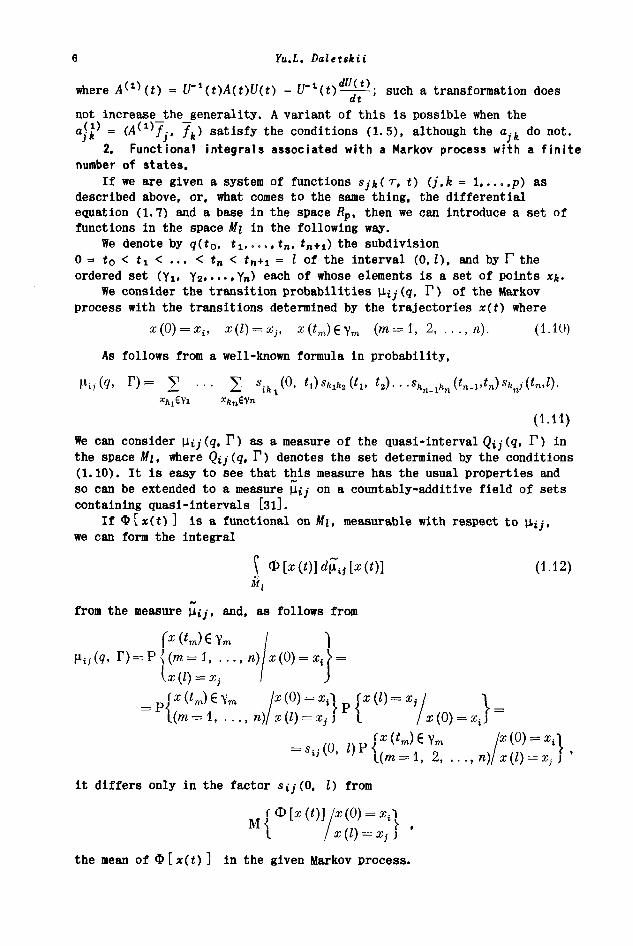
If Φ[χ(ί) ] is a functional on Mi, measurable with respect to μ^·,we can form the integral

ξ Φ[χ(ί)]άμί}[χ(ί)] (1.12)

м1

from the measure μ;,-, and, as follows from

it differs only in the factor siy(O, I) from

the mean of Φ [x(t) ] in the given Markov process.

Functional integrals connected with operator evolution equations

In order to evaluate the integral (1.12) when Φ is continuous we may-

employ a method that we describe here without demonstration, because it

will be established later in a more general case.

We consider the step-function

xo(t) = x(t

i) for i i < i < i

i + 1 (i = 0, ..., n-fl),

and let Qq[x(t)] = Φ[χ,(ΐ)] = Φ^*

1. *

2 *") be the value of Φ at x

q,

depending, of course, only on the variables xl = x(tj), (i = 1 n).

The integral of <&q[x(t)] in Mi reduces to a finite sum with respect to

the measure V-ij(q, Γ ) , induced by the measure μ^·, in the finite-

dimensional space of polygonal lines for fixed g, so that the averaging

has to be carried out only for those values of x(t) on which Q>q[ x(t) ]

depends. We see that the integral reduces to the sum

\ Фя \x (t)\ d j l . . = [ . . . \ ф а ( х \ ..., . r " ) μ ί ; ( ς , dx) =V

= Σ Σ Ф<г ( y ' ' 4 i · · · ' •*·;<„) 4 " π ι , ( 1 > , t l ) f ! k , k , ( t v t . ) . . .

• • • «/:п-11<п(^.-1' U ^ n J ^ n - I)· C1 - ' 3>

As we would expect, the mean of Φ [ * ( ΐ ) ] is obtained from that of thein the limit, as d(q) = max | tfc+i — tfe| —· 0:

i i3-= lim \ Φ 9 [x(t)] άμ^. (1.14)

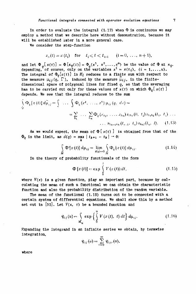
In the theory of probability functionals of the form

φ [ζ (ί)] = exp [ V(x(t))dt, (1.15)

оwhere V(x) is a given function, play an important part, because by cal-culating the mean of such a functional we can obtain the characteristicfunction and also the probability distribution of the random variable.

The mean of the functional (1.15) turns out to be connected with acertain system of differential equations. We shall show this by a methodset out in [32]. Let V(x, t) be a bounded function and

5м

и

Expanding the integrand in an infinite series we obtain, by termwiseintegration,

CO

ч>«(и)= Σ %>(«).7=0

w h e r e

Yu.L. Daletskii

Ф («) = тг ξ f \ v (·* С). О л J

), h) ... V(x(tr), ί,.)

The integral in square brackets is determined by a functional depending onthe values of x(t) at a finite number of points only, and may therefore becalculated as in (1.13):

V (r It \ t \ V (r It \ / W H —V \ 1 / > 1/ * * · \ \ г / ' г ' г i i ~~

Μ

whereF,; (0 r=V (j;,,t).

If we introduce the matrices ΨΓ = | | Ψ ΐ ; · Γ | | and V = || δ ί ; · Kj ||, we obtain

^'V<"· < r ) I 7 ( O 5 ( i r /,_,) . . . V(i,)5(i,. 0),5ο δ о .,*

from which it follows that

u

ΨΓ (и) = ξ 5 (и, t) V (t) Ψ

Γ.

Χ (ί) Λ (;• = 1,2,...).

ο00

Summing over r we obtain for the matrix Ψ = Σ ΨΓ the integral equation

r= 0и

Ψ (ц) = Ψο (и) 4- J 5 (и, t) V (t) ψ (ί) dt,

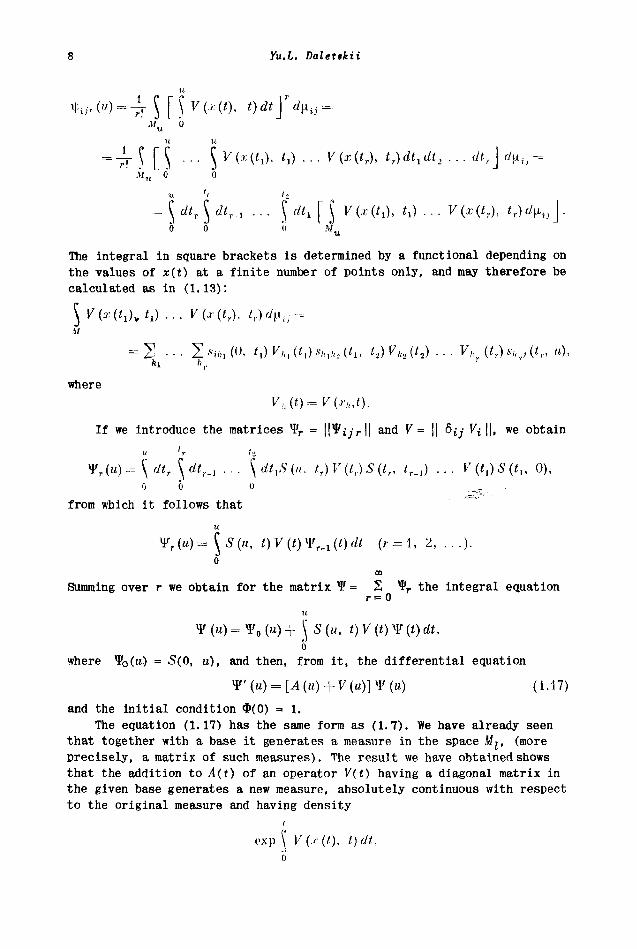
оwhere Ψ

ο(«) = 5(0, и), and then, from it, the differential equation

and the initial condition Φ(0) = 1.

The equation (1.17) has the same form as (1.7). We have already seen

that together with a base it generates a measure in the space Λ/j, (more

precisely, a matrix of such measures). The result we have obtained shows

that the addition to A(t) of an operator V(t) having a diagonal matrix in

the given base generates a new measure, absolutely continuous with respect

to the original measure and having density

ξ V(.r(t), t)dt,

Functional integrals connected with operator evolution equations 9

where V(x, t) = Vxx(t).

3. A system of differential equations not associated with a probability

scheme.

We now drop the conditions (1.5). Using (1.11) we can construct, as

before, the set-function \±ij(q, Γ ) on the quasi-intervals Qijiq, Γ ) .

However, it cannot, in general, be extended to the countably-additive field

generated by the quasi-intervals, and the integral (1.12) is not defined.

On the other hand, the construction (1.14) remains meaningful. If we apply

it to the functional (1.15) the limit exists and the matrix we obtain, as

in 2, satisfies (1.17). It is clear that the demonstration given above no

longer applies in the general case.

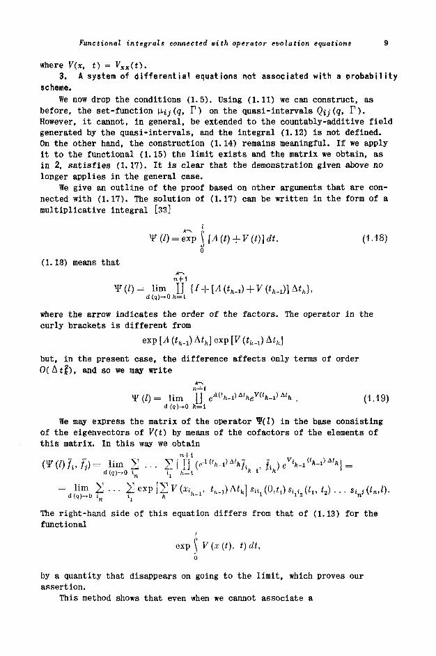
We give an outline of the proof based on other arguments that are con-

nected with (1.17). The solution of (1.17) can be written in the form of a

multiplicative integral [зз]

Y(l) = exv\[A(t) + V(t)]dt. (1.18)о

(1.18) means that

Ψ(Ζ)= Н ю "П {/ + [4(ffc_

1)+V(f

fc_

1)]Af

h},

d(g)-»0 fe=l

where the arrow indicates the order of the factors. The operator in thecurly brackets is different from

ехр[Л ( i ^

but, in the present case, the difference affects only terms of orderO(Atf), and so we may write

ψ (I) = lim "[I eA(ih-i»

Δ'*β

ν<'*-ι>

Atk . (1.19)

d (?)-»0 k=l

We may express the matrix of the operator Ψ(ί) in the base consisting

of the eigenvectors of V(t) by means of the cofactors of the elements of

this matrix. In this way we obtain

(Ψ(Ζ)/-,/-)= limd()

= l\mn Σ · • • Σ exp [ Σ V (Xi t^MJ *i4 (O.t^Siл (i l 5 ί2) . . . s t i(tn,l).

The right-hand side of this equation differs from that of (1.13) for thefunctional

exp V (x (t), t) dt,

о

by a quantity that disappears on going to the limit, which proves ourassertion.

This method shows that even when we cannot associate a

10 Yu.L. Daletskii

countably-additive measure with the differential equation (1.17) we can

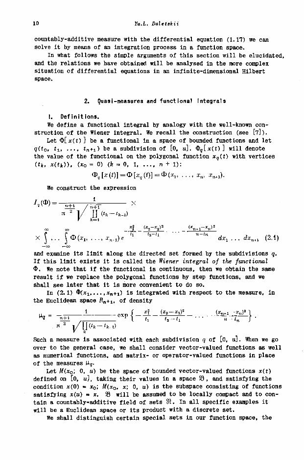
solve it by means of an integration process in a function space.

In what follows the simple arguments of this section will be elucidated,

and the relations we have obtained will be analysed in the more complex

situation of differential equations in an infinite-dimensional Hilbert

space.

2. Quasi-measures and functional integrals

I. Definitions.

We define a functional integral by analogy with the well-known con-

struction of the Wiener integral. We recall the construction (see [7]).

Let Φ[ x(t) ] be a functional in a space of bounded functions and let

q(t0, t

lt .... i

n+i) be a subdivision of [θ, u]. <&

q[x(t)] will denote

the value of the functional on the polygonal function xq(t) with vertices

(tk, x(tk)), (xo = 0 ) (k = 0, 1 η + 1):

We construct the expression

9 ч / Т"Т

я Ι/ Π («k-'fc-i)

oo oo 1_ _ 2 V _ _ n + 1 w'

VI \ ( Т ) С - Г Ύ \ P ' X '2 — ( 1 « — ί»1 , , , p . .A \ . . . X Vf ^Xj» . . . , *^n+l/ tZX^ . . . O-^-n+i \£*. l /

— OO —OO

and examine its limit along the directed set formed by the subdivisions q.

If this limit exists it is called the Wiener integral of the functional

Φ. We note that if the functional is continuous, then we obtain the same

result if we replace the polygonal functions by step functions, and we

shall see later that it is more convenient to do so.

In (2.1) Φ(*ι,...,*n+i) is integrated with respect to the measure, in

the Euclidean space i?n+i, of density

π l/lJ

Such a measure is associated with each subdivision q of [θ, u]. When we goover to the general case, we shall consider vector-valued functions as wellas numerical functions, and matrix- or operator-valued functions in placeof the measures U

9.

Let M(x0; 0, u) be the space of bounded vector-valued functions x(t)

defined on [θ, u], taking their values in a space 33 , and satisfying thecondition x(0) = x

0; M(x

0, x; 0, u) is the subspace consisting of functions

satisfying x(u) = x. S8 will be assumed to be locally compact and to con-tain a countably-additive field of sets 8Ϊ. In all specific examples itwill be a Euclidean space or its product with a discrete set.

We shall distinguish certain special sets in our function space, the

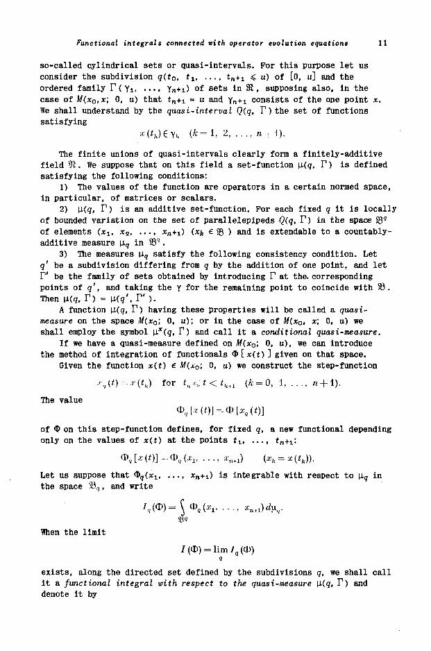
Functional integrals connected with operator evolution equations 11

so-called cylindrical sets or Quasi-intervals. For this purpose let us

consider the subdivision q(t0, *ι· ···• t

n+i - ") of [0, u] and the

ordered family Γ ( γ1( ..., γ

η+ι) of sets in Si, supposing also, in the

case of M(xo,x; 0, u) that t

n+i = u and γ

η+! consists of the one point x.

We shall understand by the quasi-interval Q(q, F)the set of functions

satisfying

Yfc (*=1. 2, ..., n+i).

The finite unions of quasi-intervals clearly form a finitely-additive

field -ft. We suppose that on this field a set-function μ(ς, Γ ) is defined

satisfying the following conditions:

1) The values of the function are operators in a certain normed space,

in particular, of matrices or scalars.

2) μ(ς, Γ ) is an additive set-function. For each fixed q it is locally

of bounded variation on the set of parallelepipeds Q(q, Γ ) in the space S39

of elements (xlt x

2 *n+i) (*fe

e 33 ) and is extendable to a countably-

additive measure \iq in S3

4.

3) The measures \iq satisfy the following consistency condition. Let

q' be a subdivision differing from q by the addition of one point, and let

Γ' be the family of sets obtained by introducing Γ at the. corresponding

points of q', and taking the γ for the remaining point to coincide with 33.

Then μ(<7, Γ ) = \x(q', Γ ).

A function \i(q, Γ ) having these properties will be called a quasi-

measure on the space M(x0; 0, u); or in the case of M(x

0, x; 0, u) we

shall employ the symbol \lx(q, Γ ) and call it a conditional quasi-measure.

If we have a quasi-measure defined on M(x0; 0, u), we can introduce

the method of integration of functionals Φ ix(t) ] given on that space.

Given the function x(t) e M(x0; 0, u) we construct the step-function

•'·.,(*)=-*·(«,.) for ih< / < i

k + 1 (* = 0, 1, ·.., n + i).

The value

of Φ on this step-function defines, for fixed q, a new functional depending

only on the values of x(t) at the points tif .... t

n+

x:

Φ,

Let us suppose that Φ,(χι *η+ι) is integrable with respect to μ7 in

the space si3

q, and write

When the limit

= Нт/,(Ф)

exists, along the directed set defined by the subdivisions q, we shall callit a functional integral with respect to the quasi-measure \J.(q, Г ) anddenote it by

12 Yu.L. Daletskii

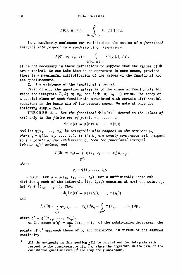
/(Φ; щ аго)= \ Ф[

3ί(χοΓθ. и)

In a completely analogous way we introduce the notion of a functionalintegral with respect to a conditional quasi-measure

/(Ф; и; x0, x)= J Φ[*(ί)]<*μ*·

ΑΓ(Χ0. '*; o, u)

It is not necessary in these definitions to suppose that the values of Φare numerical. We can take them to be operators in some space, providedthere is a meaningful multiplication of the values of the functional andthe quasi-measure.

2. The existence of the functional integral.

First of all, the question arises as to the class of functionals forwhich the integrals Ι(Φ; u; x

0) and Ι(Φ; и; x

0. x) exist. The study of

a special class of such functionals associated with certain differentialequations is the basic aim of the present paper. We note at once thefollowing simple fact.

T H E O R E M 2.1. Let the functional Φ[*(ί)] depend on the values ofx(t) only in the finite set of points τ

1 ( .... r

s:

and let φ(*ι. ..., xs) be integrable with respect to the measures \i

q,

where q = q(t0, tj. t

s). If the \l

q are weakly continuous with respect

to the points of the subdivision q, then the functional integral

Ι(Φ; и; XQ)1 exists, and

/(Ф; и; хо)= \ ф(л-

15 .(

2, . .

where

PROOF. Let q = q(t0, i i *n)· Рог a sufficiently dense sub-division q each of the intervals [tfe, tfe+i) contains at most one pointLet rk e [tik, t i f c+i). Then

and

\ ( * v · · · . з-i.) d\*q = Ι Φ (^ix. · · · . *аз4'

w h e r e q' = q'(tiv .... t i g ) .As the gauge d(q) = max | tfe+i — ijt | of the subdivision decreases, the

points of q' approach those of q, and therefore, in virtue of the assumedcontinuity,

All the arguments in this section will be carried out for integrals withrespect to the quasi-measure \i(q, Г ) , since the arguments in the case of theconditional quasi-measure μ* are completely analogous.

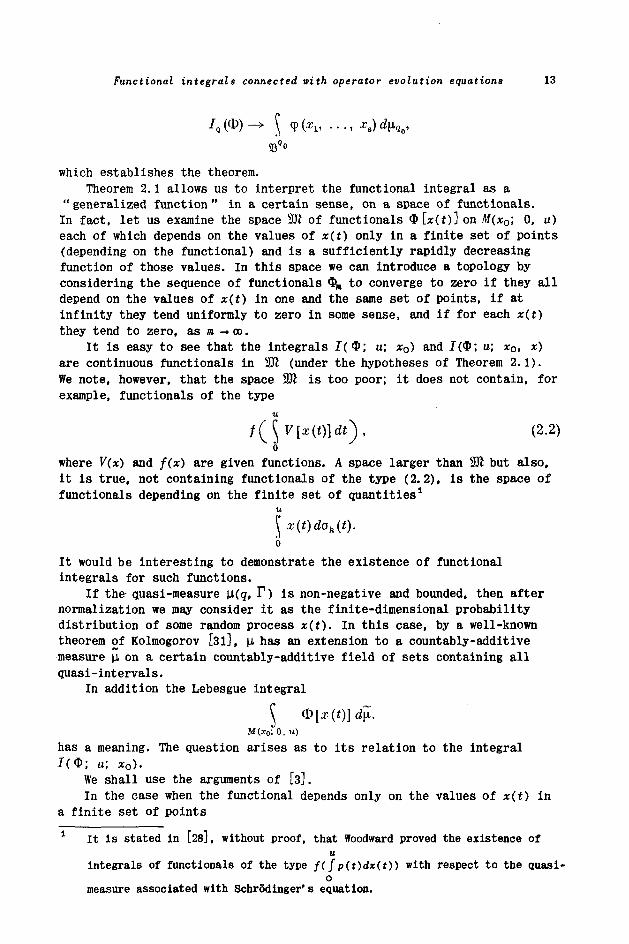
Functional integrals connected with operator evolution equations 13

which establishes the theorem.

Theorem 2.1 allows us to interpret the functional integral as a

"generalized function" in a certain sense, on a space of functionals.

In fact, let us examine the space Ш of functionals Φ[x(t)] on M(x0; 0, u)

each of which depends on the values of x(t) only in a finite set of points

(depending on the functional) and is a sufficiently rapidly decreasing

function of those values. In this space we can introduce a topology by

considering the sequence of functionals Фв to converge to zero if they all

depend on the values of x(t) in one and the same set of points, if at

infinity they tend uniformly to zero in some sense, and if for each x(t)

they tend to zero, as m — oo.

It is easy to see that the integrals Ι(Φ; и; x0) and Ι(Φ; и; x

Q, x)

are continuous functionals in ЗЛ (under the hypotheses of Theorem 2.1).

We note, however, that the space 30Ϊ is too poor; it does not contain, for

example, functionals of the type

$F[*(i)]df), (2.2)δ

where V(x) and f(x) are given functions. A space larger than 9K but also,

it is true, not containing functionals of the type (2.2), is the space of

functionals depending on the finite set of quantities1

x(t)dak(t).

о

It would be interesting to demonstrate the existence of functional

integrals for such functions.

If the quasi-measure μ(ς, Γ ) is non-negative and bounded, then after

normalization we may consider it as the finite-dimensional probability

distribution of some random process x(t). In this case, by a well-known

theorem of Kolmogorov [3l], μ has an extension to a countably-additive

measure μ on a certain countably-additive field of sets containing all

quasi-intervals.

In addition the Lebesgue integral

М(.хо;О, и)

has a meaning. The question arises as to its relation to the integral

Ι(Φ; u; x0).

We shall use the arguments of [з].

In the case when the functional depends only on the values of x(t) in

a finite set of points

1 It Is stated in [2δ], without proof, that Woodward proved the existence of

u

integrals of functionals of the type /(/p(t)dx(t)) with respect to the quasi-o

measure associated with Schrodinger's equation.

14 Yu.L. Daletskii

Φ[χ(ί)] = ψ(χ(Χι), ..., г (τ,))

and φ is integrable with respect to the corresponding measures,

; u, xo) =

follows from Theorem 2.1.

On the other hand, since in virtue of the consistency of the measures

[iq integration with respect to variables on which x(t) does not depend

leaves the Lebesgue integral with respect to μ unaltered, the latter

reduces to an integral in the space 33 ° , i.e.

M(xo;O,u) ^ д

0

Thus, for functionals of the form described above the integral

1(Ф, ц; х0) coincides with the Lebesgue integral.

In particular, for any functional Φ we have

*

Φ(Ι[χ(ί)]άμ = { Φ

4[χ(ί)]άμ. (2.3)

М(хо;0,и)

Let us assume now that for nearly all x(t), (in the sense of μ), the

relation

Ф, [ж (01·= Φ Κ (01-* Φ [«(01 f°r d(q)->0. (2.4)

is true. This is so, for instance, if μ is concentrated on the continuous

functions and Φ is continuous, but it is probably true in other cases as

well.

If some condition allowing us to pass to the limit in the Lebesgue

integral is satisfied, then the limit of the left-hand side of (2.3)

exists. Consequently, the limit of the right-hand side of that equation

also exists and coincides, by definition, with the functional integral,

also

Φ [I (i)ld?= $ Φ[χ(ί))άμ.М(х„;0,и)

In the case of certain measures associated with parabolic differential

equations we shall return to this question in §7.

3. Quasi-measures constructed from transition functions.

A probability measure connected with a Markov process is determined, in

a well-known way, by the transition probabilities of the process. We can

examine an analogous method for the construction of quasi-measures.

Let an operator-valued function

S (tlt t,; x

lt as,) (х

г, x

2 € S3; 0 < h < h< u)

(a transition function), and a measure σ(χ) be given in 93, satisfying

[ S (tt, i,; ж,, x

3) S (f

lf t

2; x

i, *„) da (x

2) = S (t

v i,;

Xl, x

3) (t, < t

2 < t

3). (2.5)

functional integrals connected vith operator evolution equations 15

We first construct a conditional quasi-measure, putting

μ| (ί> Π = 5 · · · \s Cn>

u; я».

х)

s (*п-1> *«; -υ

ж„) • · ·

... 5 (0, ίι; ж

0, а^) da (х

г) ...da (x

n).

We shall verify that the conditions of 1) are satisfied.Using the Schwarz-Bunyakovski inequality it is not difficult to

verify that in order to satisfy condition 2) it is sufficient that thefunction | S ( T , t; x, y) |

2 (τ < t) be Integrable, between finite limits,

with respect to each of the variables χ and y, and with respect to (x, y)for the corresponding measures d a(n) and d c(x) d c(y).

That 3) is satisfied follows from (2.5). In fact, if (g\ Γ ) differsfrom (q, Γ ) only by the point t', tk < t' < tfe+i, and the correspondingset γ' = 33 , then from

J s (*'> h.u »'. ; Ο 5 (i

fc. t'\ x

k, x') da (x

1) = S (t

h, t

h+1; a;

fcl x

hn)

S3

it follows easily that

Let us now set for Λ/(χ0; Ο, u)

. Π = ξ ξ ... ^ 5 (< η , ίη + 1; a;n> ж„+1) 5 (tn^, tn; x n _ v xn) . . .

. . . S (0, ij; z0> жО α?σ ( ^ . . . da(xn) da(xn^)

Here the condition 3) is verified as before if t' <In the case when t' > tn+u w

Xdo(x1)...da(xn.1)da{x')= J . .. ^ [ ξ 5 (ίη+1> f; xn+1, x')da(a:')] Xvn +i vx S3

X 5 ( ^ п . *п+ъ жп, жп+1) . . . 5 ( 0 , ^ ; ж0, о ; ! ) ^ ^ ) . . . da(a ; n t l )

and we have to postulate that

\s(t,t';x.x')da(x') = I (f < f; ζ£83). (2.6)

S3

Thus, if (2.5) and (2.6) are satisfied and \S(r, t; x, y) \2 is integrable,

the quasi-measures μ* and \is have the required properties. We note that

the functional integrals with respect to them, if they exist, are connect-

ed by a simple relation. In fact, comparing the expressions for μ5 and μ*,

we see that with tn+i = и the expression for μ«(ς, Γ ) differs from

μ*(<Ζ. Γ ) by the integration with respect to the variable x, so that

/ (Φ; a; x0) - ξ / (Φ; и; x0; χ) da (χ). (2.7)

16 Yu.L. Daletskii

We now examine the question of the extendability of the quasi-measure

\is to a countably-additive set-function.

Let us suppose first that S(r, t; x, y) is scalar-valued and, apart

from the conditions (2.5) and (2.6), also satisfies

S(x,t;x,y)>0. (2.8)

Then by the theorem of Kolmogorov quoted above, such an extension ispossible. Also, μ

8 describes the probability distribution of a certain

random process which is Markov in virtue of (2.5), in the present case,the expression of the well-known Smolukhovsky-Kolmogorov equation.

Subject to certain additional conditions, S(r, t; x, y) (theprobability density of the transition) satisfies a second-order parabolicdifferential equation, Kolmogorov's equation [зо]. More precisely, it isits fundamental solution.

A similar situation occurs if S(r, t; x, y) is not a scalar function,but a matrix one with non-negative elements. It is not difficult todetermine the probability scheme describing such a matrix function: thediffusion of a particle during which the parameter can change discretely atrandom instants of time - essentially a Markov process with two components,one discrete and one continuous. Kolmogorov's equation turns out in thiscase to be a parabolic system of equations.

In general, the fundamental solution of an arbitrary differentialequation or of a parabolic system, and also, as we shall see later, ofmore general operational differential equations, generates a functionS(r, t; x, y) satisfying (2.5), and consequently enables us to construct aquasi-measure.

It is well-known, however, that in the scalar case the fundamentalsolution of a parabolic equation of order other than two is not positive[5], [6].

The condition (2.8) is, however, not necessary for the extendabilityof μ

β. In fact, if μ

8 is real but not of constant sign, then the extension

is possible when μβ is the difference of two positive set-functions, i.e.

is of bounded variation. Extending each of the positive set-functions to acountably-additive measure we obtain the extension of μ

β. Let us examine

conditions under which this can be done.

T H E O R E M 2.2. Let the function S(r, t; x, y) be continuous withrespect to (x, y) for τ < t, and let it satisfy the conditions (2.5) and(2.6). Then a sufficient condition for the quasi-measure μ

ί in M(xo) 0, u)

to be of bounded variation is that

S Up-i-{C|5(t, t;x,y)\da(y)-i}< со (2.9)

A sufficient condition for it to be of unbounded variation is that

hm-±-\[\S(x,t;x,y)\da(y)-l\ = oo (2.10)

for each x, uniformly in τ e [θ, и ].

PROOF. 1) Let Qo be an arbitrary quasi-interval and Q

lf Q

2, .... Q

n

Functional integrals connected with operator evolution equations 17

be any family of non-intersecting quasi-intervals contained in Qo. As i sknown, u

Va^ s(£ 0) = sup2 μ8 (<?,.),3 = 1

where the upper bound is taken over all such families {Q,· I. Each of the

sets Qj 0 = 0, 1, .... n) is determined by a pair (qj.Fj). Supplementing

these pairs in a trivial manner without altering the Qj, we can arrange

for all the subdivisions to coincide. Also, all the Qj(j = 0, 1, .... n)

can be regarded as embedded in one and the same finite-dimensional space

Rq in which μs^ is dominated by the measure μι ι constructed from the

transition function |5(r, t; x, у) \ in the same way as U-s.qS( r, t; x, y). Since щ~\ is positive,

Hence i t follows thatV a r P s | 8 1 ΐ ,

The right-hand side of the last equation is, in general, increased by

augmenting the subdivision q, as |5(r, t; x, у) | does not satisfy (2.5)if (2.8) is violated. However, if (2.9) is satisfied, then for anyχ, τ, t and a certain с > 0 we have

| S (τ, t; x, y) \ da(г/)< 1 + с(t — τ ) < ec ν-

τ>,

58

which implies, in turn,

μ fs, ( & ) < J • · · J | S (t

n, t

n+l; x

n, x

M) \-\S (f

n_

lt t

n; x

n_lt x

n)\...

» 58

... | 5 (i0, t,- x

0, x

x) | da (i

x) da (x

2) ...da (x

n+1) < e

c (in.i-'n> ...

e

c ('i-V <

e™_

The first part of the theorem is thus established.

(2 From (2.10) there follows the existence of a compact set

δ(τ , t, x) such that for у е δ(τ, f; *)

5(т,<;а;,у)>0

and also

ξ S(T, f;a:, у)Лг(у)>1 + с(/-т), (2.11)6(t, <; x)

where for sufficiently small t - г, с can be made as large as desired.In fact, if S3* is the set where S(r, t\ x, y) > 0, and S3" its complement,then

^ S(T, t; x, y)da(y)- ^ S (τ, t; x, y)da{y)= ^ \S(x, t; x, y)\da(y),

S3* 58- 58

from which by (2.6) it follows that

S{x, t; x, y)da(y) = +^\ \S(x, t; x, y)\da(y).

18 Yu.L. Daletskii

This and (2.10) Imply (2.11) if we remember that we may replace S8+ by a

compact subset, decreasing the integral by an arbitrarily small amount.

We note that in the estimate (2.11) we can vary the point χ in a certain

neighbourhood V(x) without changing the set δ(τ, t; x), and also that

the quantity с may be considered independent of χ where the latter ranges

over a compact set.

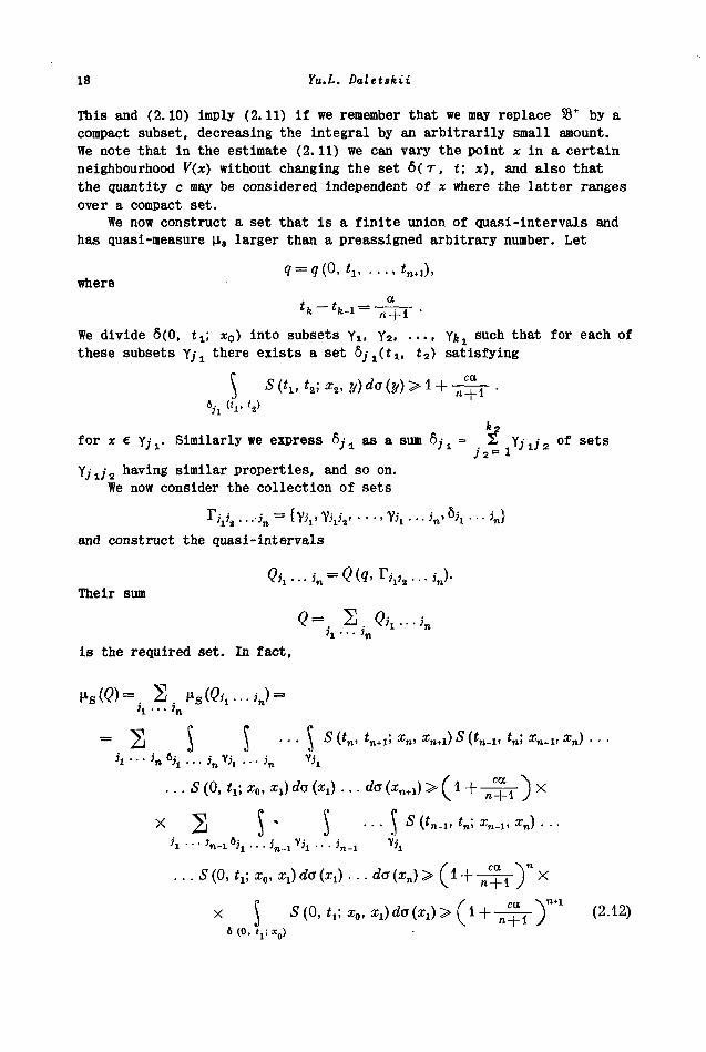
We now construct a set that is a finite union of quasi-intervals and

has quasi-measure μ5 larger than a preassigned arbitrary number. Let

where

We divide δ(0, t±; x0) into subsets Ylf γ2. . · · , Yfex such that for each ofthese subsets γ 7 ι there exists a set bj^tu t 2 ) satisfying

fe2

for χ e Yyr Similarly we express δ ; ι as a sum δ ; ι = Σ Y ; iy2 of setsη & ν

^η8 similar properties, and so on.

We now consider the collection of sets

.. ,ίη =

and construct the quasi-intervals

Their sum

is the required set. In fact,

>!···>«

. . . 5(0, ίι5 *0, daC^) . . . da(a;n+1)>(l + ^ f ) X

X 2 $ ' J · · · U 5 ('«-ι· '»"· ^n-x. *») · · ·>i •••»n-i e i 1... i n. 1vi 1... i n_ 1 \

... S (0, t i ; x0, xx) da (xO . . . da (xn) > ( l + - ^ p p ) " X

χ ξ 5(0, ίι;χ0, 1 )da(a : 1 )>( l+^ r ) " t l (2-12)β(ο. ί ^ ν

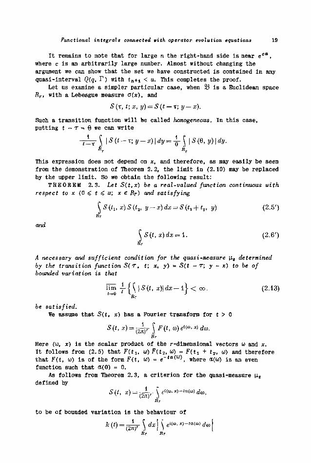
Functional integrals connected with operator evolution equations 19

It remains to note that for large η the right-hand side is near eca,

where с is an arbitrarily large number. Almost without changing theargument we can show that the set we have constructed is contained in anyquasi-interval Q(q, Г ) with t

n+i < u. This completes the proof.

Let us examine a simpler particular case, when 23 is a Euclidean spaceRr, with a Lebesgue measure σ(χ), and

S(x,t;x,y) = S(t-x;y-x).

Such a transition function will be called homogeneous. In this case,putting t - τ = θ we can write

Ar r

This expression does not depend on x, and therefore, as may easily be seen

from the demonstration of Theorem 2. 2, the limit in (2.10) may be replaced

by the upper limit. So we obtain the following result:

T H E O R E M 2.3. Let S(t,x) be a real-valued function continuous with

respect to χ (0 4 t 4 u; χ € Rr) and satisfying

S (tlt x) S (t2, y-x)dx = S(t1 + tt, y) (2.5')

Яг

and

[s(t,x)dz=l. (2.6')Rr

A necessary and sufficient condition for the quasi-measure μβ determined

by the transition function S(T, t; x, y) = S(t - т; у - χ) to be ofbounded variation is that

± { \ } a O . (2.13)

be satisfied.

We assume that S(t, x) has a Fourier transform for t > 0

Rr

Here (ω, χ) is the scalar product of the r-dimensional vectors ω and x.It follows from (2.5) that F(t

u ω) F(t

2, ω) = F(ti + t

2, ω) and therefore

that F(t, ω) is of the form F(t, ω) = <»~ί α ( ω )

, where α(ω) is an evenfunction such that <X(0) = 0.

As follows from Theorem 2.3, a criterion for the quasi-measure [is

defined by

S(t, х) = т^-уг \ ei<0)· *>-'

α<

ω> άω,

Rr

to be of bounded variation is the behaviour of

к (t) = — - \ dx \ β«ω· *)-«<*(<»> da

Rr Rr

20 Yu.L. Daletskii

near t = 0.

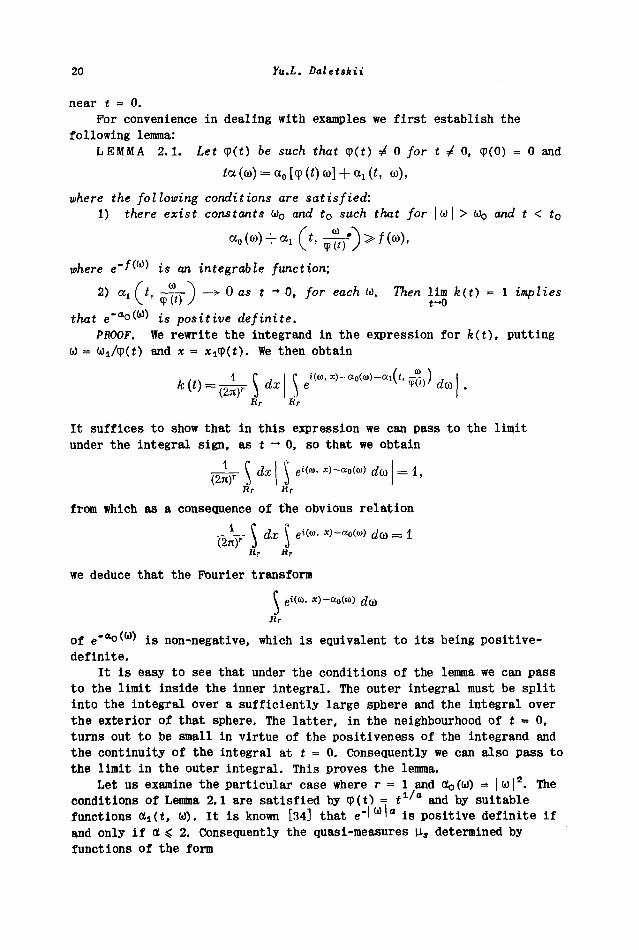
For convenience in dealing with examples we first establish the

following lemma:

L E M M A 2.1. Let cp(t) be such that cp(t) 4 0 for t 4 0, φ(0) = 0 and

] + α1(ί, ω),

where the following conditions are satisfied:

1) there exist constants ω0 ond t

0 such that for \ ω | > ω

0 and t < t

0

where e~>^ ' is an integrable function;

2) αι (*, -тггЛ - > О о! t - 0, for each ω. Then lim k(t) = 1 implies

ν Φ \ч / t-0

that β"α°^

ω' is positive definite.

PROOF. We rewrite the integrand in the expression for fe(t), putting

ω = (Oi/cpit) and χ = xiT(t). We then obtain

i(m>3C

)-a0(

ffl)-ai(t.-^)

\ \

It suffices to show that in this expression we can pass to the limit

under the integral sign, as t - 0, so that we obtain

,t(ra, χ)—αο(ω) d($ = \^

Rr

from which as a consequence of the obvious relation

1 { dx

Rr fir

we deduce that the Fourier transform

V gi(to. χ)—αο(ω) ^ω

Rr

of β"

α° ^

ω^ is non-negative, which is equivalent to its being positive-

definite.

It is easy to see that under the conditions of the lemma we can pass

to the limit inside the inner integral. The outer integral must be split

into the integral over a sufficiently large sphere and the integral over

the exterior of that sphere. The latter, in the neighbourhood of t = 0,

turns out to be small in virtue of the positiveness of the integrand and

the continuity of the integral at t = 0. Consequently we can also pass to

the limit in the outer integral. This proves the lemma.

Let us examine the particular case where r = 1 and οίο(ω) = |ω|2. The

conditions of Lemma 2.1 are satisfied by (p(t) = t1^" and by suitable

functions OLi.(t, ω). It is known [34] that β-1

ωι

α i

S positive definite if

and only if ot < 2. Consequently the quasi-measures \is determined by

functions of the form

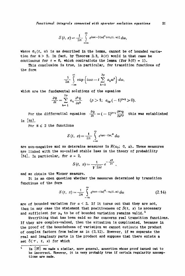
Functional integrals connected with operator evolution equations 21

where a^t, ω) is as described in the lemma, cannot be of bounded varia-

tion for α > 2. In fact, by Theorem 2.3, k(t) would in that case be

continuous for t = 0, which contradicts the lemma (for k(0) = 1).

This conclusion is true, in particular, for transition functions of

the form

oo 2p

~2— \ exp < ΐωχ — t 2 аъ.®

к \

ω>

-оэ ft=0

which are the fundamental solutions of the equation

ft= 1

For the differential equation -^- = (— l ) p + 1 this was established

in [35].For a 4 2 the functions

are non-negative and so determine measures in M(x0; 0, u). These measuresare linked with the so-called stable laws in the theory of probability[34]. In particular, for α = 2,

and we obtain the Wiener measure.It i s an open question whether the measures determined by transit ion

functions of the form

S (t, x) — -l— С βιω*-ί|ω|α-αι(ί. ω) ω (2.14)—οο

are of bounded variation for a < 2. If it turns out that they are not,

then in any case the statement that positiveness of S(t, x) is necessary

and sufficient for μβ to be of bounded variation remains valid.

1

Everything that has been said so far concerns real transition functions.

If they are complex-valued, then the situation is complicated, because in

the proof of the boundedness of variation we cannot estimate the product

of complex factors from below as in (2.12). However, if we separate the

real and imaginary parts in the product and suppose that there exists a

set δ ( τ , t, x) for which

In [27] we made a similar, more general, assertion whose proof turned out tobe incorrect. However, i t is very probably true if certain regularity assump-tions are made.

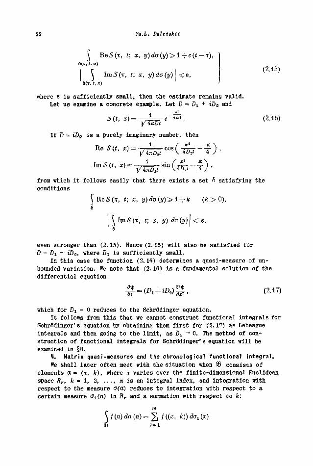
22 Yu.L. Daletskii

«(τ, f.χ)

, t; x, y)da(y)>\

Ιπι5(τ, ί; χ, у) da (у)

β(τ, ί,

(2.15)

where ε is sufficiently small, then the estimate remains valid.

Let us examine a concrete example. Let D = Dt + iD

2 and

S(t, x) = .1 4£>t (2.16)

If D = iD2 is a purely imaginary number, then

from which it follows easily that there exists a set δ satisfying the

conditions

, t; x, y)da(y)>i (Λ > 0),

, t; x, y) da{y)< ε,

even stronger than (2.15). Hence (2.15) will also be satisfied for

D = Di + iD2. where Di is sufficiently small.

In this case the function (2.16) determines a quasi-measure of un-

bounded variation. We note that (2.16) is a fundamental solution of the

differential equation

(2.17)

which for Dt = 0 reduces to the Schr6dinger equation.

It follows from this that we cannot construct functional integrals for

Rchr6dinger' s equation by obtaining them first for (2.17) as Lebesgue

integrals and then going to the limit, as Di -* 0. The method of con-

struction of functional integrals for Schrodinger's equation will be

examined in §Я.

4. Matrix quasi-measures and the chronological functional integral.

We shall later often meet with the situation when 85 consists of

elements ot = (x, k), where χ varies over the finite-dimensional Euclidean

space Rr, k = 1, 2 m is an integral index, and integration with

respect to the measure σ(α) reduces to integration with respect to a

certain measure σ^η) in Rr and a summation with respect to k:

m

/(a) da (a) = 2 /((*, tydo^x).

Functional integrals connected vith operator evolution equations 23

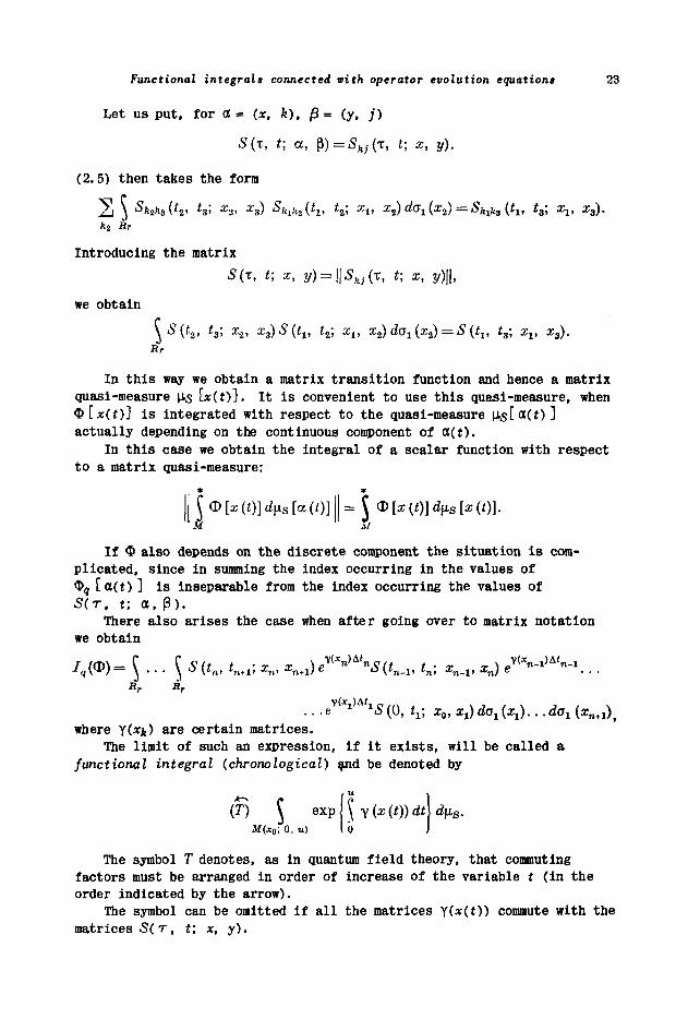
Let us put, for ot = (x. k), /3= (y, j)

S(x, t; α, β) = 5Μ,(τ, ί; χ, у).

(2. 5) then takes the form

2 3 ' W s (*г< *з> X2> хз) shih2(tv h\ xv хг)dcfi(x2) = Shlhs (flT t3; xx, x3).

k R3

k2 Rr

Introducing the matrix

S(x, t; x, y) = \\Skj(x, t; x, y)\\,

we obtain

\S(t2, t

3; х

г, x

s)S{t

v i

2; х

г, х

2) da

1(x

2) = S (t

17 t

3; x

v x

3).

Rr

In this way we obtain a matrix transition function and hence a matrix

quasi-measure Us ix(t)]. It is convenient to use this quasi-measure, when

Φ[*(£)] is integrated with respect to the quasi-measure Us[<X(t)]

actually depending on the continuous component of ot(t).

In this case we obtain the integral of a scalar function with respect

to a matrix quasi-measure:

II f Φ [χ (t)] άμ8 [α (t)] \\=\Φ[Χ (ί)] άμ

8 [χ (ί)]·

If Φ also depends on the discrete component the situation is com-

plicated, since in summing the index occurring in the values of

Фд [d(t) ] is inseparable from the index occurring the values of

S(r, t; α, β ) .

There also arises the case when after going over to matrix notation

we obtain

= ξ . . . \ S(tn, t n + 1; xn, xn+1)ey{Xn)AtnS(tn_u tn; xn_v xn) e

v C

R R

<*η-ΐ>Δίη-ι

...eyXl *S (0, tx; x0, xx) dat (arj ...da1 (а;п + 1) ?

where Y(xk) are certain matrices.The limit of such an expression, if i t exists, will be called a

functional integral (chronological) and be denoted by

(Τ)Μ(χ0. ο, «)

The symbol T denotes, as in quantum field theory, that commuting

factors must be arranged in order of increase of the variable t (in the

order indicated by the arrow).

The symbol can be omitted if all the matrices Y(x(t)) commute with the

matrices S(r, t; x, y).

24 Yu.L. Daletskii

3. Basic and generalized elements of Hubert space

I. Spaces of basic and generalized elements.

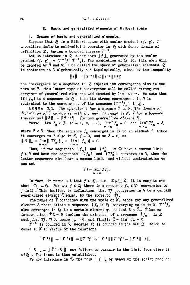
Suppose that $ is a Hilbert space with scalar product (/, g), Τ

a positive definite self-adjoint operator in ig with dense domain of

definition φ , having a bounded inverse Γ"1.

Let us introduce in a new norm ||/||. generated by the scalar

product (/, g) . = (T"1/. T~

1g). The completion of £> for this norm will

be denoted by N and will be called the space of generalized elements.

is contained in N algebraically and topologically, since by the inequality

the convergence of a sequence in ig implies its convergence also in the

norm of N. This latter type of convergence will be called strong con-

vergence of generalized elements and denoted by lim" or -*. We note that

if {/„ \ is a sequence in Jg , then its strong convergence in N is

equivalent to the convergence of the sequence {T~1f

n ! in φ .

L E M M A 3.1. The operator Τ has a closure f in N. The domain of

definition of Τ coincides with $£•, and its range is Ν. Τ has a bounded

inverse and ||£||_ = Hf"1^!! f

or апУ generalized element £.

PROOF. Let fn e φ (η = 1, 2. . . . ) , lim" f

n = 0, and lim" Tf

n = £,

η -* со η -. со

where £ e N. Then the sequence fn converges in i§ to an element /. Sinceit converges to / also in N, f = 0, and so £ = 0, as||S ||. = lim||r/n||.= lim || /„ || = 0.

П — CD П -» CO

Thus, if two sequences {/ ! and \ f'n\ in Φ have a common limit

f e N and both the sequences ( Tfn ! and { Tfn \ converge in N, then the

latter sequences also have a common limit, and without contradiction we

can set

In fact, it turns out that f e φ , i.e. ® ^ Я. &· It is easy to see

that φ,« = φ . For any / e !Q there is a sequence /n« S converging to

/ in φ . This implies, by definition, that Tfn converges in iV to a certain

generalized element £ equal, by the above,to Tf.

The range of f" coincides with the whole of N, since for any generalized

element £ there exists a sequence {/„} С Q converging to it in N. T" 1fn

also converges in to a certain element φ, so that £ = Tip. Τ has an

inverse since f S, = 0 implies the existence of a sequence {fn ! in Φ

such that Tfn 0, hence /„ - 0, and finally £ = lim" f

n = 0.

f1"

1 is bounded in N, because it is bounded in the set ί§ , which is

dense in N in virtue of the relations

II 5 II- = II TN"

1£ II

n o w follows by passage to the limit from elements

of^ . The lemma is thus established.

We now introduce in Φ the norm || / ||+ by means of the scalar product

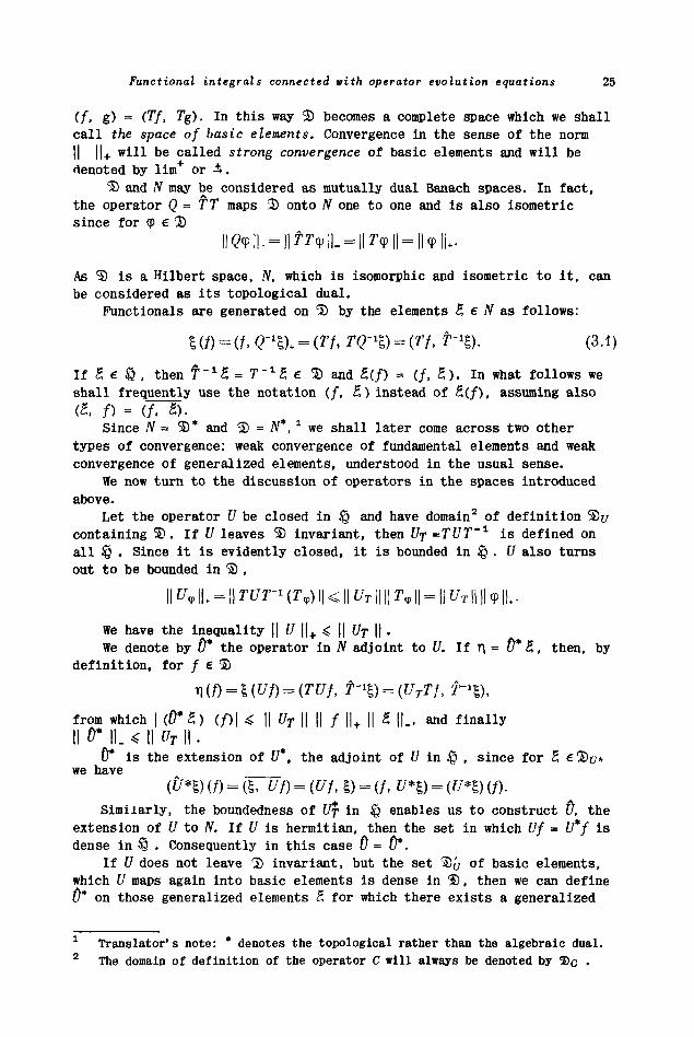
Functional integrals connected with operator evolution equations 25

(f> g) = (Tf· Tg). In this way Φ becomes a complete space which we shall

call the space of basic elements. Convergence in the sense of the norm

|| ||+ will be called strong convergence of basic elements and will be

denoted by lim+ or -i.

Φ and N may be considered as mutually dual Banach spaces. In fact,

the operator Q=TT maps ® onto N one to one and is also isometric

since for φ e Φ

As Φ is a Hilbert space, N, which is isomorphic and isometric to i t , canbe considered as i t s topological dual.

Punctionals are generated on Φ by the elements £ e N as follows:

I (/) - (/. <ГЧ)* = (77, TQ-4) = (Г/, т-Ъ). (3.1)

If Ζ € & , then f " 1 5 = 7 T - 1 5 e ® a n d £(/) = (/,£). In what follows weshall frequently use the notation (/, £) instead of £(/), assuming also(£, f) = (/, S).

Since iV = Φ * and Φ = Ν*, * we shall later come across two othertypes of convergence: weak convergence of fundamental elements and weak

convergence of generalized elements, understood in the usual sense.

We now turn to the discussion of operators in the spaces introduced

above.

Let the operator U be closed in i§ and have domain2 of definition Ф у

containing Φ . If U leaves Φ invariant, then UT =TUT

mi is defined on

all £? . Since it is evidently closed, it is bounded in ф . U also turns

out to be bounded in Φ ,

|| U91 = II TUT'

1 (Τ

φ) ||< II U

TII || Τ

φИ = II U

TII || Φ ||

+.

We have the inequality || U ||+ < || U

T ||.

We denote by 0* the operator in N adjoint to U. If η = 0* Β , then, by

definition, for / e Φ

from which \ (0* £) (f)\ 4 \\ UT \\ \\ f ||

+ || I || , and finally

II 0" ||. < || UT || .

ϋ* is the extension of U*, the adjoint of U in $ , since for 5we have

ФФ ч ) (/) = (I, ut) = (c//, i) = (/, U*D = (t/

Similarly, the boundedness of Uj· in enables us to construct 0, the

extension of U to iV. If U is hermitian, then the set in which Uf = iff is

dense in Й . Consequently in this case ϋ = 0*.

If if does not leave Φ invariant, but the set Фу of basic elements,

which U maps again into basic elements is dense in Φ , then we can define

0* on those generalized elements £ for which there exists a generalized

1 Translator's note: * denotes the topological rather than the algebraic dual.

2 The domain of definition of the operator С will always be denoted by © c ·

26 Yu.L. Daletskii

element r\ such that

ξ (СЛр) = η (φ)

for all φ e Φ ύ . r\ = б* £ is uniQuely defined. The operator 0* may in this

case be unbounded in N.

Later we shall frequently meet operators U satisfying

\\TUT\\<ao. (3.2)

The following result holds for them:L E M M A 3.2. If the operator U satisfies (3.2), then 0 and U* map N

into © , and A

ί/ / (ξ,ηζΛΟ. (3.3)

PROOF. 0 and и are defined and bounded in N, because by the condi-

tions of the lemma ϋγ and Щ are bounded in 6 · Let £ e N, £* e ©

(fe = 1. 2, ...) and linf£fc = 5. This means that Τ " * £

fc - f "

1 £ , and

к -.со

since ΤUΤ and ί/ Τ are bounded, then

C/ξ, = (UT) (T-^h) -^ UT (f-4) = Ul,

TUlh = (Γί/Γ) (Γ"1!,,) -> Γί/Γ (Τ"1!).

From the fact that Τ is closed it now follows that 0 £ e Φ and

TUT (Γ"1!) = 2'C>|.

In this manner we can also prove that и £ e Ъ . Lastly

? f ), 7Г1Л) = (^, TU*T (Γ^η)) =

REMARK. It follows from

II f/1 | | t = II TUt II = II TUT ( 7 4 ) || < || TUT || || ξ | | .

that under the conditions of the lemma U maps a strongly convergentsequence of generalized elements into a strongly convergent sequence ofbasic elements.

2. Complete systems of generalized elements.

Let £x be a set of generalized elements depending on the parameter χ

varying in a space 5B in which a measure a(x) is defined.With each basic element φ we associate a function on 85 :

<p(z) = U<P) = (<P,!*). (3.4)

We suppose that the following conditions are satisfied:

1) for any φ e Φ

со.

2) for any ψ, φ e

(φ, ψ) = ^ φ (χ) ψ(χ) άσ (χ) = ^ (φ, ξχ) (ξ

χ, ψ) da (x). (3.5)

The family £* will then be called a complete system of generalized

Functional integrals connected with operator evolution equations 27

elements.

(3. 5) means that any basic element φ may be represented In the form

φ = \ (φ, lix)l-

xda(x), where the integral converges weakly in N.

93

(3.4) and the condition (3.5) establish a one-to-one and isometric

mapping between Ъ , with the i§ metric, and a certain space ®σ of functions

on 58 with the metric induced by the scalar product

\ φ (ζ) ψ {x) da {x).

93

Extending this mapping by continuity we obtain a similar mapping

between ig and a certain function space ί§σ which is a subspace of 82,0.

the space of functions on Ъ square-integrable with respect to the measureO(x). Let us now suppose that !Q

O coincides with 2

2>cr. This will be true,

for example, if 2)σ contains all sufficiently smooth functions or any

other family of functions dense in 22,σ· Рог the element of ί§σ corres-

ponding to / e <g we have

Finally let us extend the correspondence to the generalized elements,by associating with each generalized element η the generalized functionr\(x), (which we shall also denote by the symbols 5* (η) and (η, £*)),defined by

93

also expressable in the form

= (ii,q>) (φζΦ). (3.6)

93

The space of functions η(χ) will be denoted by Νσ.

We shall examine ®o and N<r with the topologies induced by the

topologies of 2) and N, respectively. We shall call ®σ the space of basic

functions and No- the space of generalized functions.

We shall always suppose that a certain class К of functions on Ж existswith the property that multiplication by them is continuous in Фо . In otherwords, if a(x) e К and A is the operator in ® defined by

Αφ — \ α (χ) φ (χ) \

χ da (x)

23for the element

93

then A is bounded in Ъ .The class К can consist, for example, of bounded functions having a

certain degree of smoothness and satisfying certain boundary conditions.

28 Yu.L. Daletskii

Let us examine the form of an operator in Sg after transition to $Qa .

Let В be an operator in for which Βγ = Τ ВТ'1 is bounded. Then

the generalized element r\x = B*£

x is meaningful and so also the generalized

function

Similarly if Βγ is bounded, we can define the generalized function

y(x) = e {x, y) = (lx, Bl

y) Щ Г п

The generalized functions b(x, y) and c(x, y) will be called generalizedkernels corresponding to the operator B.

If φ e © and ψ e ® , then the expressions

$ 6 (x, y) φ (у) da (у) = J (£*ξ*, |y) (Е„, φ) da (у) = (B*l

x, φ) = (ξ,, Я

Ф). (3.7)

SB SB

ψ (*) [ J Ь (*, 2/) Ф Й da (у) ] ώσ (χ) = ξ (ψ, У (ξχ, Β

φ) da (χ) = (ψ, Β

φ) (3.8)

8 S3 93

are meaningful and so are

c(x, y)*(z)da(x)=^W, ξχ)(ξ

χ, Л|

у)йа(х) = (г);, £ξ

Β) = (β*ψ, ξ

υ), (3.9)

S3

$ [ J с (χ, y)*(x)Ar(a!)] ψ (у) da (у) = J (β·ψ, ξΒ)(ξ

Β, φ) da (у) = (β·ψ, φ).

(3.10)The right-hand sides of (3.8) and (3.10) are equal but we cannot concludethat the kernels b(x, y) and c(x, y) coincide, because, generally speaking,we may not change the order of integration in the left-hand sides of theequations.

We now examine certain operations that we can carry out on generalizedkernels.

1) Let a(x) be a function in the class К and let A be the boundedoperator in ® corresponding to it. If c(x, y) is the generalized kernelcorresponding to B, then

ca(

x> y) = a(x)c(x, y)

is the generalized kernel corresponding to A*B (it is easy to see that A*is the operator of multiplication by the function a(x)).

In fact, putting Ψι = Αψ, we have for any ψ e Φ

[ ψ (χ) ca (χ, у) da (χ) = ξ ψ! (χ) с (χ, y) da (χ) = (5*ψ

χ, ξ.) =

« 83

= ( 5 Μ ψ , ξ.) = \ (ξ,, A*Bta) ψ (χ) da (χ).

2) Let Ci,(x, у) = (&х, В

гВ.

у) and c

2(x, у) = (5*, Вг^у) be two

generalized kernels. We examine their convolution

c(x, z)= [c^x, y)c2(y, z)da(y).

Functional integrals connected with operator evolution equations 29

where the integral is understood in the weak sense. It is also ageneralized kernel, corresponding to the operator В^В

2:

In fact, for φ e Ъ we have

\* φ (χ) с (χ, ζ) da (χ) = jj [ jj φ (χ) сг (χ, у) da (χ) j с2 (у, ζ) da (у) =SB SB

= (φ, fiAU= ξ ff(x)(lx,B

1B

tlz)da(x).

58

3) Let α^χ), ..., αη(χ) be functions in if, and let c^{x, у)

··•. cn(x, у) be generalized kernels. If we apply in turn the operations

examined above, we find that

К (Xo, x) = [ • • • \ C

x (ж

0.

(3.11)

where the integrals are understood in the weak sense and are taken in theorder indicated by the differentials, is also a generalized kernel. Thiskernel, as is not difficult to verify, corresponds to the operatorBtAtB^l ... A*

n.xBn.

So far we have talked of generalized kernels. However, under certainconditions which we shall now examine, they are ordinary functions.

Let TBT be bounded. Then in accordance with Lemma 3.2

and so the kernel

c(x, y) = UI t ΒΙ

is a basic function in χ and also in y.

Let us recall that the quantity

is called the absolute norm of the operator B, where fk (fe = 1, . · . , n,is an orthonormal base in i§. As is well-known, || В ||

ff does not depend on

the choice of the base. Operators having a finite absolute norm areusually called Hilbert-Schmidt operators.

L E M M A 3.3. If В is a Hilbert-Schmidt operator and || TBT || < oo,then

\\В\\И= [ \\Ь{х, у) |

2 da (χ) da (у). (3.12)

PROOF. Let φ e 'ЗЗ and Βφ = /. Then

30 Yu.L. Daletskii

= J (φ, 1у)(1у, B*tx)do(y)=\ (Bly, у (φ, ξ,) da (г/).58 58

In this way, instead of an abstract operational equation, we obtain anintegral equation in 22.a-

/(ж)= b(x, у) ψ (у) da {у).

58

Since the mapping φ - <p(y) is an isometric representation of £> on

S2, σ> the operator В is unitarily equivalent to the integral operator

with kernel b(x, y). We thus obtain (3.12), since that relation is true

for Hilbert-Schmidt operators.

We shall later meet with the case when the operators Β(ε), depending

on ε, are such that for ε > 0 ΤΒ(ε)Τ'1 is bounded and, as ε -· 0,

β (ε) —> В (0)

in the sense of strong convergence in 2), and Β(ε) satisfies the condi-

tions of Lemma 3. 3 for ε > 0.

By virtue of that lemma all the integrals in the formulae (3.7)-(3.10)

converge absolutely for ε > 0. Because of this we may change the order of

integration in them and so the kernels of the form b(x, y, ε) and

с(х, у, ε) coincide.

The generalized kernels b(x, y, 0), c(x, y, 0) in this case are weak

limits of the corresponding kernels b(x, y, ε), с(х, у, ε), as ε -* 0. Prom

this follows that in the given case b(x, y, 0) and c(x, y, 0) also coin-

cide.

We note that the generalized kernel K(x0, x, 0) (see (3.11)) deter-

mined by the operators Β^(ε) (k = 1, 2 n) of the type described

above is also the weak limit of the corresponding kernels K(x0, χ, ε) in

which all the integrals converge absolutely.

Let us agree on the following notation for use later. In the case when

the ct = (x, k) are elements of the space 33, as described in §2.4, we

shall consider the function

φ(α) = (φ, ξα) = (φ, l

xh) = <p

ft (ж) (Л=1, ..., г)

as vector-valued, and write

Equation (3.5) in this case is written in the form

(φ, ψ) = \ (φ (ж), ψ (χ)) do1 (x),

Κwhere the sign ( ) denotes the scalar product in Д

г.

Similarly we shall consider the kernel

as a matrix, and use the notation

Functional integrals connected vith operator evolution equations 31

b i x , y) = \ \ b k j { x > y)\\-

3. Generalized eigen-elements of self-adjoint operators.Let В be a self-adjoint operator in a space £> and E( Δ) be the

corresponding spectral set. Let us recall what this means [Зб], [37].£ ( Δ ) is an additive operator-valued function of the interval Δ

satisfying the following conditions:1) the Ε(Δ) are projectors, i .e.

2) the Ε(Δ) commute with В and form a complete orthogonal set in thesense

£(Δ1)£(Δ

2) = £ ( Δ

1Π Δ

2) , Ε ((-co, oo)) = 1.

3) the following representation holds for functions of В as an

abstract Stieltjes integralCO

/(Β)ψ = \ 1(x)dEx^ (3.13)— CO

for ψ e Φ/(Β;· Alsooo

\ , 4>) (3.14)

and Ф/(в) consists of the ψ for which (3.14) converges.If f(x) is bounded on the spectrum Λ

β of B, then the operator f(B) is

bounded and

||/(B) || = sup |/(ΐ)|.лв

We say that В has a simple spectrum if there exists an element u(generating element) such that the vector subspace generated by the setof elements E(A)u is dense in £.

In this way we define, for the characteristic functions of intervals,

a correspondence

f(x)-»f(B)u

between the functions and elements of the Hilbert space & . Extending this

correspondence by continuity we obtain by virtue of (3.14) an isomorphic

and isometric correspondenceoo

^ f(x)dExu = f(B)u (3.15)

between the space of functions square-integrable with respect to the

measure σ(Δ) = (Ε(Δ)ιζ, u) and the space Jg.

The application of an operator of the form φ(Β) to an element of Sg

reduces after transition to йг.о to multiplication by the function φ(*).We note that σ(χ) is called the spectral function (measure) of the

operator B.

If no element u having the property described above exists, then,

32 Yu.L. Daletskii

taking an element ux and considering the closure of the vector spacegenerated by the elements £(Д)и

1( we do not obtain the whole spaced ,

but only a subspace Jgj . Choosing u2 e£) Q ^ and proceeding as before we

obtain ig2 , and so on.Let us assume that there is a set of elements ult u2, ..., un for

which the above process breaks off, i. e.

where m is a minimal number of vectors for which such a decomposition ispossible. In this case we say that the multiplicity of the spectrum of Вis m.

For any / e Sg , if В has spectrum of multiplicity m, we have the

expansion

m m

where P^ is the projector onto the subspace

& ( A = l , . . . , /ra), u = u1+...+um, uk = Phu.

The operators Pk (k ~ 1, .. ·, m) commute with B.

In this way we obtain a correspondence between φ and the space β ™σ

of vector-valued functions (fx(x), .... f

n(x)) with the norm

II /II1 = Σ I \fk(*)\'da

k(x),

ft=l - G O

where ak(A) = (E(H)u

k, щ) = (E(b)P

ku, a).

Each of the measures σ^(Δ) is concentrated on a certain set 50ift. It

turns out that the generating elements can be chosen so that the measures

Ok are the projections on the ЗКЙ of one and the same measure σ.

Рог suppose that o(x) = o±(x) + ... + о

я(х), say. Then each of the

measures Ok(x) (k = 1, .... m) is absolutely continuous with respect to

o(x), i.e. is representable in the form

= Jwhere Δ is any set measurable with respect to o(x), and μ^ is a summable

function. On the other hand, as is well-known, there exists a measure pj,

concentrated on a set 9ϊΑ of zero σ* -measure and such that

σ (Δ) = V λ, (χ) doh (χ) -I-

Qk (Δ Π%),

Δ

where λ*(*) is summable with respect to Ok(x). It is not difficult to see

that outside the set 3lk[j3lk, where -J is the set at points in which

\ik(x) = 0, which also has zero σ*-measure, we have \fe(at) = ΐ/μ*(*). It

follows from this that the function

Functional integrals connected with operator evolution equations 33

vft(x)=

I 0, when

is summable with respect to the measure Ok(x).Let us now take as new generating elements

"ft = 5 V v h ( ж ) d E x u h (A = 1, 2, . . . . m ) .—m

QO

Any vector of the form fk = fh(B)uk= [ }u(x)dExuk is now written—oo

/ь = \ 4h{x)dE

xu'

k, where the function cp

h(a-) = f

k(x)J/ μ,,(:ε) is square-

summable with respect to the measure da'h(x) = а(Е

хщ, u'

k) = v

k(x)da

h(x).

On the set 33ife = M

h — 9l

fe — iJU the measures σ^ and σ coincide.

Thus Sg can be mapped onto the space of vector-valued functions

where /jfe(x) is square-summable with respect to σ(*) and equal to zero

outside 3J?h. This representation gives the formula

ft=l

moreover

со

||/||2= \ ((f(x)))

2da(x),

-co

where

ft=1

Let us suppose now that В has the following property:(III.l) Рог any finite interval Δ, Γ "

1^ ) is a Hilbert-Schmidt

operator.

Then, as is shown in [is], there exists inJVa set of elements

(-oo < χ < oo; k = 1, 2, ..., m) such that, for the basic elements φ, the

mapping of !g onto £2,0 described above is given by the formula

Ф И * ) = (Φ. Sfe*)· Also it is clear that

from which it follows that the generalized elements { Zkx \ form a complete

set in the sense of 2. Let us agree to consider B,kx = 0 if x£Wh . Then

we may regard the integrals in (3.16) as extended to the whole axis

-00 < χ < 00. Here the space 93 consists of the points (x, k), where

34 Yu.L. Daletskii

X € Π1 ( k = 1, ···, IB.

The Ekx &re generalized eigen-elements of В In the following sense.Let g(*) be a function for which there exists in Φ a dense set Ъ'

д mapped

by g(B) into basic elements

Then

(g(B)4,lx) = g{x)to,tx) (Ф6ЭД- (3.17)

(3.17) means that £x is in the domain of definition of g(B)* and

Let us formulate certain conditions which we shall assume to besatisfied in the following exposition.

(III.2) There exists a class F of functions g(x) having the propertythat for each of them © contains a dense subset %'g of ig such that

F contains at least the characteristic function of intervals.(111.3) F contains a subset Flf also dense in Sg , having the property

фр = ф , i.e. g(B) φ с φ for all g б ίΊ· The subset Flt may consist, for

example, of functions having a certain degree of smoothness.(111.4) The generating elements can be chosen so that they belong to

Φ. Also ^ Ф С Ф -If the generating elements satisfy (III.3) and (III. 4), they also

satisfy the conditions

(uh,l

jx) = \j (k,j = l,...,m). (3.18)

It is sufficient to show this in the case when the spectrum of В is simple.

For any interval Δ and any function f(x) e F± vanishing outside Δ we have

CO CO

I!» = $ \(f(B)u,U\2da(x)= ξ \(и,Г{В)*1

х)\*аа(х) =

A

On the o t h e r hand, || f(B)u\\2= f \f(x)\2 d a ( x ) . Comparing t h e s e twoΔ

expressions the required relation follows.In the definition of a generating element we do not use the element

itself, but the elements of the form E(A)u. We can therefore consider ageneralization of the concept, the so-called improper generating elements[38]. We give the relevant definitions.

We shall call the set of elements {\|/д} an improper element of thespace Jg associated with the operator B, where Δ is an arbitrary finiteinterval, if it has the properties:

1) £(Δ)ψΔ.= ψ

Δ;

2) for Δ Π Δ' = 0, ψΔ + ψ

Δ» = ψ

Δ υ Δ/

We write ψΔ = Ε(Δ)ψ and call ψ

Δ the projection of the improper element

Functional integrals connected with operator evolution equations 35

ψ onto the subspace ίρΔ = #(Δ) Jg.

Let Λ be an operator for which \)/д e Φ Α . Let us suppose that the

limit

φΔ= lim £(Д)Л\|>д<,

Δ'—>ϋχ

exists, where flt = (-00, ω ) , and also that <рд = Ε(Δ)Αψ. The elements фд

clearly define a new improper element φ, which we write φ = Λψ.The expression фд, as is easy to see, has a meaning if A satisfies

the conditionΕ (Α) Α = Ε (Δ) ΑΕ {&') (3.19)

for each interval Δ, with a certain Δ' depending on Δ. In particular, this

condition is satisfied if the operator commutes with the spectral set

£(Δ), for example if it is a function of B.

Let us assume that В has a simple spectrum. If ψ is an improperelement, then for each Δ the function ψ^Οκ) exists,

The set of functions Щ(х) is consistent in the sense that on the commonpart of the intervals Δ and Δ' the functions ψ^ί*) and \|/д< (χ) coincidealmost everywhere in the sense of the measure o(x). We introduce a

function ψ(χ), square-summable with respect to a(x) in each finite

interval and coinciding with each of the Щ(х) in its domain of definition,and we write

. (3.20)

It is easy to see that when ψ(χ) e 2г,о» the element ψ is a properelement.

Thus, the space S of improper elements is an extension of $Q, and in

the mapping on & onto £2,σ goes into a space of functions locally square-

summable with respect to o(x).

The sequence ψη e 15 (n = 1, 2, ...) will be called convergent if for

each Δ, {ψη. ! converges strongly in £>. We note that if 33 is dense in ig ,

then we can always construct a sequence ψη еЗЗ, converging strongly to the

improper element ψ.

Let us now generalize the definition so as to give meaning to Λψ when

ΨΛ с ΦΑ.We shall say that the improper element ψ belongs to the extended domain

of definition Ί>Α of A if there exists a sequence ψη e Ъ

А (η = 1, 2, ...)

convergent to it and such that the sequence Ε(Δ)Αψη has a limit Фд е

for all Δ. This definition is consistent if £(Δ)Α has a closure, and (3.19)holds for those elements for which the right-hand side is defined.

We shall call the improper element u a generating element for В if theclosed vector subspace generated by its projections Я(Л)ц coincides withSQ. It is not difficult to see that all the concepts mentioned above inconnection with ordinary generating elements extend also to this case,with the exception of the fact that the spectral measure o(x) will nowonly be locally of bounded variation. The expression (u, £„) can in this

36 Yu.L. Daletskii

case be defined by

where f(x) is in the class Flt does not vanish at x

0, and is chosen so

that f(B)u e ®. It is not difficult to verify that the result does not

depend on the choice of function.

The construction described in this section admits the following

generalization. Instead of one operator we can consider a set

Βλ, B

2, .. ., B

n

of commuting self-adjoint operators with the spectral sets Ει(Δ),£2(Δ) £η(Δ). If Δ ( η ) i s an η-dimensional interval with " s i d e s "Δι, Δ

2, ..., Δ

η, then putting

£(Δ<ω) = ^ ( Δ

χ) . . . Ε(Α

η),

we introduce an operator-valued measure in the space Rn. If we integrate

with respect to it a function f(x) given in Rn we shall obtain operators

which are functions of Blt B

2 B

n:

f ( B l t . . . , B n ) = J fix,, x t , ..., xn)dE™.

We can also examine a more general case when we are given directly a

certain operator-valued function of sets Ε(Δ") in Rn having properties

analogous to those of a spectral set described at the beginning of this

section. Then the operators of the form

5 f(x)dE (3.21)

form a commutative ring that is not, in general, generated by operators

Bit .... B

n. We shall call these operators functions of the spectral set

Ε(Δη).The concepts examined above, generating elements and multiplicity, are

related, as is easy to see, to properties of the spectral set, and so go

over to this new situation. The space $ in this case maps onto a space

of functions given in Rn or into some domain (3C R

n.

It turns out that all the results of [18] go over to this case without

modification, and so there exists a sets of generalized elements

S,kx (x e Rn> k = 1, 2, ...) that are generalized eigen-elements of the

operators of the form (3.21) in the same sense as in the one-dimensional

case.

Ц. Examples.

1) Let Q be the space %•> of functions square-summable on the realaxis with respect to the Lebesgue measure. As operator Τ we choose the

closure of the differential operator (-1) -r-^ + 1 considered on twice

continuously differentiable finite functions. The space 5) of basic

elements coincides with the space W% (-00,00) of functions square-

integrable together with their derivatives of order up to 2k inclusive.

The space N consists of generalized functions, in the sense of S.L. Sobolev,

Functional integrals connected with operator evolution equations 37

of order 2k.

If В is the operator of multiplication by the independent variable x:

Bf(x) = xf(x),

then the delta-functions £Xo = δ(χ - x

Q) are its generalized eigen-

functions, where

(/. l.xo)= f(x)6(x-x

o)dx = f(x

o).

The condition (III.1) is satisfied for k = 1, 2, .... as the operator

T'1 has a continuous kernel square summable with respect to each of the

variables, (Carleman kernel).

2) Similarly we can consider the case $ = £2(a, b), where (a, b) is а

finite or infinite interval. As operator Τ we can take the operatorgenerated by a differential expression with any self-adjoint boundary

conditions. In the case of a finite interval (a, b), T'1 has also a

finite absolute norm, in the case of an infinite interval the situation is

as above. The delta-functions δ(χ - x0) for x

0 £ (a. b) form a complete

set of generalized eigen-elements for the operator of multiplication by *.

The class F± in the first and second examples consists of the functions

differentiable a sufficient number of times and bounded, together with

their derivatives, (we shall call such functions sufficiently smooth).

3) Now let Jg = S2 (R

n) and let Τ be the closure, on the set of

sufficiently smooth finite functions, of the operator

where Δ is the Laplacian.

Let us examine the commuting set of operators Blt B

2, .... B

n of

multiplication by the variables xit *

2 x

n> respectively. The n-n

dimensional delta functions tx> = δ(χ - χ') = Π δ(XJ - χ}) form a

; = 1complete system of generalized eigen-functions of these operators.

For sufficiently large k, k > π/4, 7 "1 is an integral operator with

a Carleman kernel, and so condition (III.1) is satisfied.It is clear that instead of R

n we may consider any domain in the

space and in it the operator Γ with any self-adjoint boundary conditions.Instead of the functions of B

t B

n we shall have to examine the

commutative ring of operators of multiplication by the functions/(*!, .... X

n).

For k > η/4, Τ'1 has a Carleman kernel.

4) In each of these examples we can consider, instead of the space

of scalar functions, the space of vector-valued functions with values in

Rn. The generalized functions of the form

Sta- = (0, .... b(x-x'), 0, ..., 0),

where there is a non-zero component in the fe-th position, form a completeset of generalized eigen-elements.

5) Let us examine, in the space 8™ [ a. b] of vector-valued functionsf(x) with values in Д", the operator

38 Yu.L. Daletskii

(Af)(x) = a(x)f(x)

of multiplication by a self-adjoint matrix function a(x). We shall deter-

mine its generalized eigen-elements.

Let \kW and /fe(x) be the eigenvalues and eigenvectors of the matrix

a(x). Let us suppose that [a, b] can be divided into a finite set of sub-

intervals Mk. Ml Jl/£ifc) (fe = 1. 2, .... m) in each of which X

k(x)

varies monotonically and has a non-vanishing derivative. Then in each of

the MJ (j = 1, ..., ik', k = 1, .... m) the function Xfc(jc) has an inverse

*jkO§ defined on a certain set Affc.

Now we set

ξ<Γ> (χ) = δ (λ, (χ) - μ) fh (χ) Δ,·, (χ), (3.22)

where

The £$J*^ form a complete set of generalized eigen-elements of A. In

fact

A$h) (x) = A

i h (ж) δ (λ, (я) - μ) α (χ) f

k (χ) =

= Aj h (χ) X

h (χ) δ (λ, (χ) - μ)/, (χ) = μξ«

Μ {.τ),

and, as is easy to see, for fixed j, k there are no other generalizedeigen-elements corresponding to μ, since λ^(χ) is monotone in the intervalwhere hjk(x) 4 0.

We now verify that the set is complete. The scalar product of thevector functions

/ (x) = Σ «F, (x) h (x), g И - Σ %ft ft

can be written in the form

ь\ fk (χ) Μ ^ Σ

ft о ft j nf j

h

Let us change the variable in each of the integrals on the right, puttingχ = xjk(b) and Fj

k(K) = φ*(*/*(λ)), Gj

fc(\) = ψ

Λ(χ

;·^(λ)). Then we obtain

(/, g) = 2 \ Fik (λ) G

ift (λ) | x-

h (λ) | <ίλ. (3.23)

i. ft A .f t

On the other hand,

ж) μ) Ajh(/, Εμ) = j φ,, (ж) δ (λ, (ж) - μ) A

jh (χ) dx =

= 5

δ (λ ~μ)

( Ь («ih (μ)) νΊ*5*(μ)Ι. _ if μ 6 \jk,

I 0, if μζΛ^,

Functional integrals connected with operator evolution equations 39

and therefore, by (3.23), there follows the required relation:

The situation is rather more complicated when the functions inquestion depend on a vector argument χ e R

n.

We shall suppose that in each domain Mjk the invertible change ofvariables

is possible, also

k)h = Xh (s = l, .. ., n; / = 1, . . ., ih; к = 1, . . ., m).

When we take in hjk(x) instead of the derivative the Jacobian

, λ ,..., л,")w e c a n г е р е а ^ ^ n e arguments developed above. However, we

D (x1, x

2, ..., x

n)

do not obtain a complete set of generalized eigen-elements automatically.In order to obtain such a set we select in the variety Л(„) containing allthe Ajb (j = 1, ..., ijt; k = 1, ..., n) the set of functions У (λ

1, ..., λ

η) ,

orthonormalized with respect to the variables λ2, ..., λ

η, for each fixed

λ1, and put

l\l' k'r) = Y)k (x) УЬ^ЩЬ (λ, (χ) - μ) fh (x),

where

It is not difficult to verify that the system so obtained is complete.

Ц. Evolution equations

I. The resolvent operator.

In §2 it was noted that in the construction of a quasi-measure we can

make use of the fundamental solutions of differential equations of para-

bolic type. We shall see that we can associate a similar construction with

a general equation in a Hilbert spaceig

where ψ e Й and H(t) is a closed operator in .In this section we shall examine those properties of the equation (4.1)

needed for such a construction.Our arguments will be based on certain conditions which we now

formulate, and in the following sections we shall elucidate the cases inwhich they are satisfied.

Firstly it will always be assumed that the following condition issatisfied:

(IV.1) For 0 4 τ 4 t 4 и there exists a bounded operator U(t, τ),strongly continuous with respect to t and satisfying U( r, τ) = I.

If ψ0 e ®Η(τ) then ψ(ί) = U(t, τ) ψ

0 e ® н « ) for t > т. The vector

40 Yu.L. Daletskii

ψ(ί) is strongly differentiable for t > r, satisfies (4.1), and is theonly solution of that equation having such properties.

The operator U(t, τ) satisfying (IV.1) will be called the resolventoperator of the equation (4.1).

Prom the uniqueness of the solution it follows at once that it hasthe property

U(t, x) = U(t, s)U(s, x) (r<s<i). (4.2)

In certain cases it will also be assumed that the following condition

is satisfied:

(IV. 2) The operator Я™ is defined, and for ψ0 e Ф

ят (τ)

If ff"(i) is closed, and H~m(r) is bounded, then this condition is

equivalent to the boundedness of

Hm(t)U(t, x)H-

m(x).

The last of the conditions of this type is the strongest.(IV. 3) For t > τ the operators TU(t, τ) and U(t, τ)Τ, where Τ is the

operator used to construct the spaces of basic and generalized elements,are bounded.

It follows from (IV.3) and (4.2) that for t > r.TU(t, τ)Τ = TU(t, s)U(s, τ)Τ is bounded.

Hence by Lemma 3.2 we can conclude that 0(t, τ) and U*(t, τ) exist andoperate continuously from N to Ъ .

If in (4.1) Я does not depend on t, then for the existence of theresolvent operator, which we shall in this case denote by

U(t, τ) = 6Η('-

τ>.

it is sufficient for Я to satisfy the well-known Hille-Yosida conditions[β]. We do not formulate these conditions as we shall examine a smallerclass of operators whose properties we shall have to study in moredetail.

In any case they are automatically satisfied if Я is normal and itsspectrum lies to the left of a certain vertical line. e

Ht can be con-

structed using the formula

eBi = [ e

u άΕ

λ, (4.3)

л

where Εχ is the spectral set of Я and Λ its spectrum. If Λ lies to theleft of some vertical line then for t > 0 the function β

λ ί is bounded on

Λ and hence efft is bounded. Since it commutes with H, it is clear that

(IV. 1) and (IV. 2) are satisfied.This is true, in particular, if Я = гН

1г where H

± is self-adjoint.

If Η is self-adjoint and non-positive then, on its spectrum, λΓβ * is

bounded for any r - 0. Hence for any r > 0 and г > 0

< со. (4.4)

Furthermore, if Я satisfies the condition:

Functional integrals connected with operator evolution equations 41

(IV.4) || ГЯ"Г|| < oo for any r > 0, then it follows from (4.4) that

the condition (IV. 3) is satisfied.

For (4.1) with variable H(t) having constant domain Ί)Η, the condi-

tions for the existence of the resolvent operator are to be found in [9].

Without formulating these conditions we note that they are satisfied if,

for any t, H(t) is normal, its spectrum lies to the left of some vertical

line, and for ψ e ® н the vector H(t)y is strongly continuously differen-tiable with respect to t.

In particular we may consider the case when H(t) = i#i(f), where#i(f) is self-adjoint, or when H(t) is self-adjoint and non-positive. Ineach of these cases (IV.1) is satisfied. Sufficient conditions for (IV. 2)and (IV.3) to be satisfied will be described below.

We note that in fe] U(t, τ) is constructed with the help of the formula

U(t, т) = ПтПеЯ ('*-

1 ) Л'\ (4.5)

q * = 1

where q(t0, t

lt .... t

n) is a subdivision of [τ, t], and the limit is

understood in the strong sense under the condition that the gauge d(q) of

the subdivision q tends to zero.

2. The equation with an additional term of lower order.

Below we examine basically operators of the form

H(t)=—A(t) + B(t), (4.6)

assuming that A(t) satisfies one of the conditions described in the

previous section, and B(t) is strongly continuous and is either bounded or

of fractional order with respect to A(t), which in that case is supposed

positive definite.

We say that В is of fractional order with respect to the positivedefinite operator A [ll], if for any γ < 1,

||Λ4-Ί|<οο. (4.7)

The equation (4.1) for operators of the form (4.6), satisfying (4.7)

(abstract elliptic operators) is studied in [ll]. Since the. properties of

the resolvent operator of such an equation are used below in an essential

way, and there are, among them, some which are not formulated explicitly

in [ll], we indicate their demonstration, the more so since in [ll] the

proofs are only outlined. This is relative to certain results from [ίο].

Firstly we shall prove the following:

L E M M A 4.1. Let A and С be setf-adjoint positive definiteoperators and В an arbitrary operator such that

IIяU< oo, ιμ^-ι|Ι<«.

Then for 0 < ν < 1 the operator AVBC~V is bounded, and

PROOF. We use the following result of Heinz [39]. If Л and С are self-adjoint operators and Q is a linear operator satisfying

IIρ/IKIIc/II for||<?*Л1<1М/И for

42 Yu.L. Daletskii

then

Let us put, in th i s inequality. C / = u, f e %c and A1"1^ = v. g e ®A-Then u e © c i_v and u € ΦΑν· Prom the equality

Ι (ρ/, 4V-Io)|<!icv/||.||B||it follows that the left-hand side is continuous with respect to v, and

so Q/ е ФА, _

( and 1 (A

V~1QC~

Vu, v) \ ζ \\ и \\ \\ υ \\. which implies

H^-^C^Il^l. (4.8)

To prove the desired result we take, in this inequality,

Q = 1 AB,where/c = max {|| В ||; || ABC'1 \\}.

We then obtain

|| A"'1 ABC" ||< к.

REMARK. Using arguments similar to those of [40] we can show that if

А, В, С depend on t in such a way that B(t) and Аа)Ва)С"ха) are

bounded and strongly continuous, and if in addition the domains of

certain fractional powers of A(t) and C(t) are constant, then

Av(t)B(t)C-

v(t) (0 < V < 1) is strongly continuous.

We can now prove the following theorem:

T H E O R E M 4.1. Let A(t) be a positive definite operator, B(t) an

operator satisfying, for a certain m and ye [ 0, l ] , the conditions

|| В (t) A~y (i) || < C, || A

n (<) В (t) A (i)~

n"

v ||< C, η = max (m - 1,1) (4.9)

and suppose the operators occurring in these inequalities are strongly

continuous.

Let U(t, τ) be the resolvent operator of the equation

(4.10)

Then if the condition

\\Ar+a{t)U(t, ΐ)Λ'

Γ(τ)||<'Μ|ί-τΓ

α (4.11)

is satisfied for 0< α < 1 - γ and 0 ^ г < в - 1, the resolvent operatorV(t, τ) of the equation

i£ H, (4.10')

exists and we have the inequality

| | Ar (t) V it, x) A-* {x)\\<M1 \t-x |-<r->

for all 0 -$ s < r < m - γ. V(t, r) and Ar(t)V(t, т)А"

в(т) are strongly

continuous with respect to t for t > т.

PROOF. We note firstly that by the remark after Lemma 4.1 there

follows from (4.9) the boundedness and strong continuity of the

operators

Functional integrals connected with operator evolution equations 43

Αμ (t) В (t) Α~μ~ν (t) (0<μ<Λ).

Equation (4.10*) is equivalent to the integral equation

t

V (t, x) = U(t,x) + U (t, s) В (s) V (.9, τ) ds.χ

Let us consider the integral equation

t

Υ(ί, τ) = Ar (t)U(t, τ) A'

r (τ) + ^A

r(t) U(t, s) A~

(r-

y)(sr)Я

А(*) У (s, x)ds, (4.12)

where Bx(s) = A

r~

7(s)B(s)A~

r(s) is bounded for 0 4 r 4 m - -1. Prom the

estimate|| A

T(t) U (f, s) A~

(r-y) (s) \\<M(t-s)~

y

it follows that this latter integral equation has a summable kernel and so

its solution is bounded, strongly continuous, and can be obtained by the

method of successive approximations. It is easy to verify that

Now from (4.12) we obtain

Ar+e (t) V (t, x) A~

r (τ) = A

r+e (0 U (t, χ) Α'

τ (τ) +

t

[Ar+e (f) U (t, s) A~

(r-y) (s)] B

x (s) Υ (s, x) ds,

x

which, for ε < 1 - γ, gives, in virtue of

|| Ar+S (t) U (t, x) A-

r (τ) || < Μ \t - χ \~\

|| Ατ+ε (t) U(t, s) A~

{r-y) (s)\\<M\t-s Γ

( ε + ν )

the estimate

\\Ar+e(t)V(t, T)A-

r(x)\\<M

1\t-T\-*

Now choose η so that ε = —-— < 1 - γ. Then we have forη

s 4 r < m - у, tk = t - k *—^-, the relationП

Ar(t)V{t, x)A-

s(x) =

= [AT(t)V(t, i ^ - ^ y i r ' W f i i . ί

2)^-

Γ+2ε(ί

2)]...

. . . [ ^ i + e («„.,) F («„.!, x)A-(x)],

from which there follows the estimate

|| AT (t) V (t, x) A-s (τ) || < M?nrs 11 - τ |-0-·>.

This completes the proof.REMARK 1. If we suppose that A(t) is an arbitrary operator for which

(4.10) has a resolvent, then the theorem, with <X = Υ = 0 and r = s, remainstrue.

REMARK 2. If B*(t) satisfies the condition (4.9) then we can, by

44 Yu.l. Daletskii

similar arguments, obtain the estimate

|| A-s (t) V(t,x) Ατ (τ) || < Μ, j t - 1 1 - <'->.

REMARK 3. The boundedness of A(t)B(t)A~1~'

y (t) for m = 1 is necessary

in order that B(t)i4"r(t) shall leave Φ Α ( Ο invariant. The integral

equation we examine is equivalent to (4.10'). We may weaken the condition,requiring only that B(t)A'

y(t) be bounded, but we then have to assume, in

addition, that it is smooth with respect to t, for example, that itsatisfies a Lipschitz condition (see [12]).

C O R O L L A R Y 1. If for a certain r < m - γ the condition \\ ΓΛ"Γ||< οο

is satisfied, and if В and В* satisfy (4.9), then V(t,r) satisfies thecondition (IV.3).

In fact we have

TV it, x) = TA-T(t)[A

r(t)V(t, τ)], V (t, x)T = [V(t, τ) Α* (τ)] A'

T (τ) Τ,

and thus the operators we consider are bounded.C O R O L L A R Y 2. If the equation (4.10) has a resolvent operator

satisfying the conditions (IV.1, 2), and if B(t) satisfies (4.9) forγ = 0, then the equation (4.10') satisfies (IV. 1, 2).

Here we do not assume that A(t) is positive definite.Making use of the hypotheses we note at once that the operator

where A is a self-adjoint operator, and В satisfies (4.9) for γ = 0,satisfies the conditions (IV.1, 2), replacing fl* by Λ". If Л and В satisfythe conditions of Corollary 1 then

g(-A+B)f

satisfies the condition (IV. 3).These assertions remain valid in the case when A is a constant

operator and В = B(t) depends on t.We now turn to an examination of the conditions under which the

resolvent operator of (4.1), with variable A(t), has the properties(IV.2,3). We shall consider only the case where the domain Φ Α of A(t)does not depend on t.

We first obtain an estimate generalizing (4.4).L E M M A 4.2. Let A(t) be positive-de finite and have domain Φ

Α not

depending on t, and suppose A'(t)A'1(t) is bounded, and strongly continuous.

Then we have the estimate

\\A«(t)U(t, χ)Α->{τ)\\< [-^L]-*^'-»2? (4.13)

PROOF. We first examine

. ( ) D8=1

t — τwhere tk = т + k , and estimate the bound of the operator

Functional integrals connected with operator evolution equations 45

Aa(t)Un(t, τ)Α-*{χ) (0<β<α<1).

Рог this we represent i t as a product

A*(l)U,(t. »)-4" fW-

s = l

and estimate the factors. Prom (4.4) it follows that

α—Β i—x α-β

Рог the bound of the second factor we note that from the evident

relation ts

< S - 1

there follows the estimateN

(t J 4-i (f,.0 | |< 1 + *=? tf < e»

where ]V = max | | A'(u)A"1(t) Ц . In [39] the inequality is established,

" ' * || A» (ts) A"» (t^) |j< [|| A (i.) -i (ί,.0 | | f (0 < μ < 1),

Finally we obtain

8 = 1

"lot—β N(t —τ) // л /

Г77—ϊγ e 2

· <4·

14·

It remains to show that the estimate holds also for U(t, τ). By the

conditions of the Lemma A(t)U(t, Ό Α "1^ ) is bounded. Using Lemma 4.1 we

can conclude that Aa(t)U(t, r)A'

a(r) are also bounded. We now examine the

sequence of vectors

yn - A* it) U

n (f, τ) A~

a (t) χ {χ € β).

I t is bounded by (4.14), snd so we can extract a weakly convergentsubsequence ynk. Since for ν e Φ Α α ( ί )

(Упк, v) = (Un(t, x)A-«(x)x, Aa(t)v)->(U(t,x)A~a(t)x,Aa(t)v) =

= {Aa(t)U(t, x)A~a(x)x, v),

we havel i m y n = y = Aa(i)U (t, χ) Α~α(τ)χ.ft->oo ft

Finally, for л; е φ ρ_α we obtain the inequality

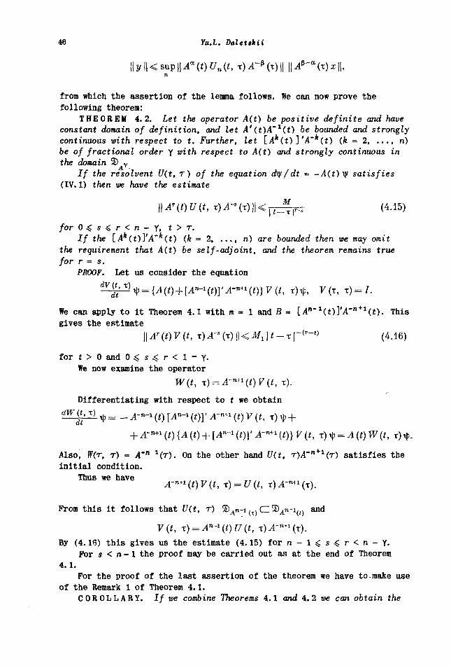
46 Yu.L. Daletskii

|| у | | < sup || Aa(t) Un(t, τ) A~* (τ) || || Α*~α(τ)χ ||,η

from which the assertion of the lemma follows. We can now prove the

following theorem:

T H E O R E M 4.2. Let the operator A(t) be positive definite and have

constant domain of definition, and let A'(t)A"i(t) be bounded and strongly

continuous with respect to t. Further, let lAk(t)]'A"

k(t) (k = 2 n)

be of fractional order γ with respect to A(t) and strongly continuous in

the domain © Y

If the resolvent U(t, r ) of the equation dy / dt = -A(t) ψ satisfies

(IV. 1) then we have the estimate

\\Ar(t)U(t, т)Л-(т)|Кр^7]гТ (4-15)

for 04s4r<n-V, t > r .If the [i4*(t)]'A"*(t) (fe = 2 n) are bounded then we may omit

the requirement that A(t) be self-adjoint, and the theorem remains truefor r = s.

PROOF. Let us consider the equation

(t, ΐ)ψ, V(T, τ) = /.

We can apply to it Theorem 4.1 with m = 1 and В = [An*

1(t)]'A"

n+1(t). This

gives the estimate

\\Ar(t)V(t, x)A-

t(x)\\<M

1\t-x\-<

r-

l> (4.16)

for t > 0 and O^:s.$r<l-Y.

We now examine the operator

W(t, x) = A~™(t)V(t, τ).

Differentiating with respect to t we obtaindW£*) tf τ)ψ +

t, τ)ψ.

Also, W(r, r) = Д"п 1(т). On the other hand U(t, т)Л-"

+1(г) satisfies the

initial condition.

Thus we have ^ (<) F (/> т ) β

^ (/> т )

-n+1 ( τ )

Prom this i t follows that U(t, τ) ΦΑη-ι ( t ) CZ ®An-i ( ( ) and

7(i, x) = An~l(t)U(t, x)A-™(r).

By (4.16) this gives us the estimate (4.15) for n-14s4r<n-Y.

For s < n-1 the proof may be carried out as at the end of Theorem

4.1.

For the proof of the last assertion of the theorem we have to make use

of the Remark 1 of Theorem 4.1.

COROLLARY. If we combine Theorems 4.1 and 4.2 me can obtain the

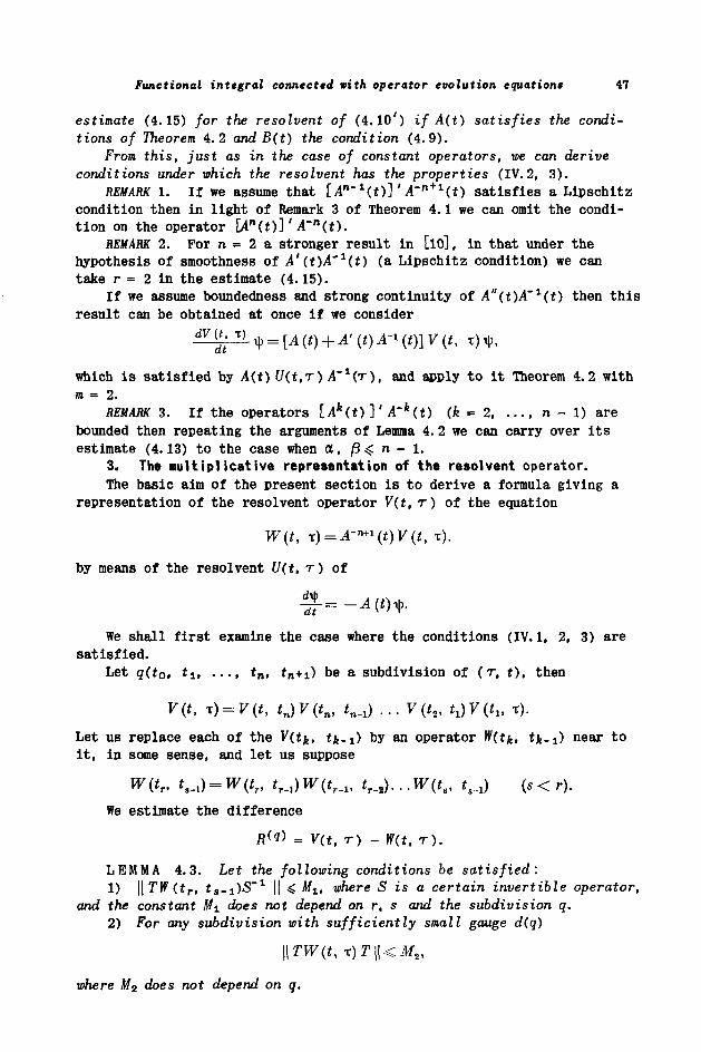
Functional integral connected with operator evolution equations 47

estimate (4.15) for the resolvent of (4.10') if A(t) satisfies the condi-

tions of Theorem 4.2 and B(t) the condition (4.9).

From this, just as in the case of constant operators, we can derive

conditions under which the resolvent has the properties (IV. 2, 3).

REMARK 1. If we assume that [An'

1(t>]' A"

n + 1(t) satisfies a Lipschitz

condition then in light of Remark 3 of Theorem 4.1 we can omit the condi-

tion on the operator [An(t)]' A'

n(t).

REMARK 2. Рог η = 2 a stronger result in [ίο], in that under the

hypothesis of smoothness of A'(t)A~x(t) (a Lipschitz condition) we can

take г = 2 in the estimate (4.15).

If we assume boundedness and strong continuity of A"(t)A'1(t) then this

result can be obtained at once if we consider

which is satisfied by A(t) U(t,r) A~1(r), and apply to it Theorem 4.2 with

m = 2.

REMARK 3. If the operators [Ak(t) ]' A~

k(t) (k = 2, ..., η - 1) are

bounded then repeating the arguments of Lemma 4. 2 we can carry over its

estimate (4.13) to the case when α , β 4 η - 1.

3. The multiplicative representation of the resolvent operator.

The basic aim of the present section is to derive a formula giving a

representation of the resolvent operator V(t, r ) of the equation

W(t, x) = A-»"(t)V(t,x).

by means of the resolvent U(t, r ) of

We shall first examine the case where the conditions (IV.1, 2, 3) aresatisfied.

Let q(t0, fit · · · . *n» *n+i) be a subdivision of (τ , t ) , then

V(t, x) = V(t, tn)V(tn, t^) ... V(tt, tJV(tlt x).

Let us replace each of the V(tk, tk-i) by an operator W(tfc, tfe-i) near to

it, in some sense, and let us suppose

W(tr. t,_J = W(t

r, t^Wit^, t

r_

2)...W(t

s, t^) (s<r).

We estimate the difference

Я<»> = V(t,r) - W(t.r).

LEMMA 4.3. Let the following conditions be satisfied :1) | |T№(t r , i j . i ) ^ 1 | | ^ Mlt where S is a certain invertible operator,

and the constant M± does not depend on r, s and the subdivision q.2) For any subdivision with sufficiently small gauge d(q)

\\TW(t,x)T\\<Mit

where M2 does not depend on q.

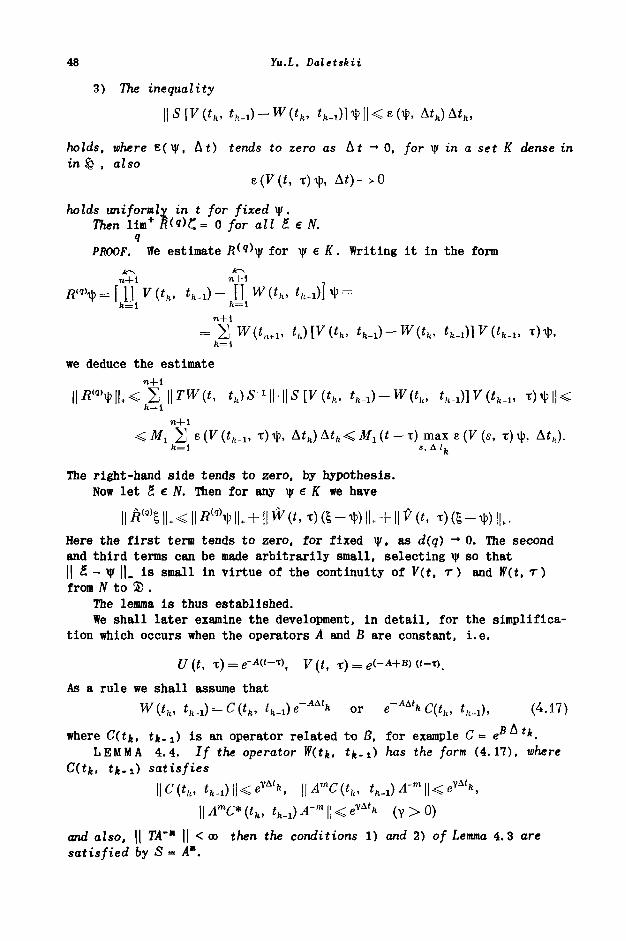
48 Yu.L. Daletskii

3) The inequality

\\S[V(tk, th^)-W{tk, ί ^ ΐ Ψ ί Κ ε ί ψ , Atk)Ath,

holds, where ε(ψ, Δι) tends to zero as At -· 0, for ψ in α set К dense inin £) , aZso

i, τ) ψ, Δί)-^0

holds uniformly in t for fixed ψ.77ien lim

+ fi(9)£ = 0 for all I e N.

яPBOOF. We estimate fl

(9)\|/ for ψ e К. Writing it in the form

n+l n+l

η+1, th)[V(th, tk^)

we deduce the estimaten+l

| |Λ ( 9 >Φ|Ι+< Σ \\TW(t, th)S-i\\.\\S[V(th, t^-W^, «„.О] V («„.ρ τft=l

n+l

< ^ ι Σ e(V(i fe.i, τ) ψ, Aift) Aih < ϋ/χ (< - τ) max ε (V (s, τ) ψ,ft=l s, Δ / f t

The right-hand side tends to zero, by hypothesis.Now let Ζ e N. Then for any ψ e К we have

Here the first term tends to zero, for fixed ψ, as d(q) — 0. The secondand third terms can be made arbitrarily small, selecting ψ so thatII £ - Ψ IL is small in virtue of the continuity of V(t, τ) and Y/(t, r )from N to 2) .

The lemma is thus established.We shall later examine the development, in detail, for the simplifica-

tion which occurs when the operators A and В are constant, i.e.

U(t, х) = е~А«-

х\ V(t, x) =

e<.-

As a rule we shall assume that

W(th,t

k_

1) = C(t

k,t

h_

1)e-

AAtb or e-

AAtkC(t

h, i^j, (4.17)

where C(ife, tk-i) i s an operator related to B, for example C= eB tk.LEMMA 4.4. If the operator W(tk, tfe-i) has the form (4.17), where

C(tfei tfc-i) satisfies

\\C(th, ί,,ΛΙΚβ '*, |ИтС(^, i ^ ^ I K e ^ ,MmC*('fe. i ^ ^ - I K e ^ (γ>0)

and aZso, || TA~* \\ < oo then the conditions 1) and 2) of Lemma 4.3 aresatisfied by S = A".

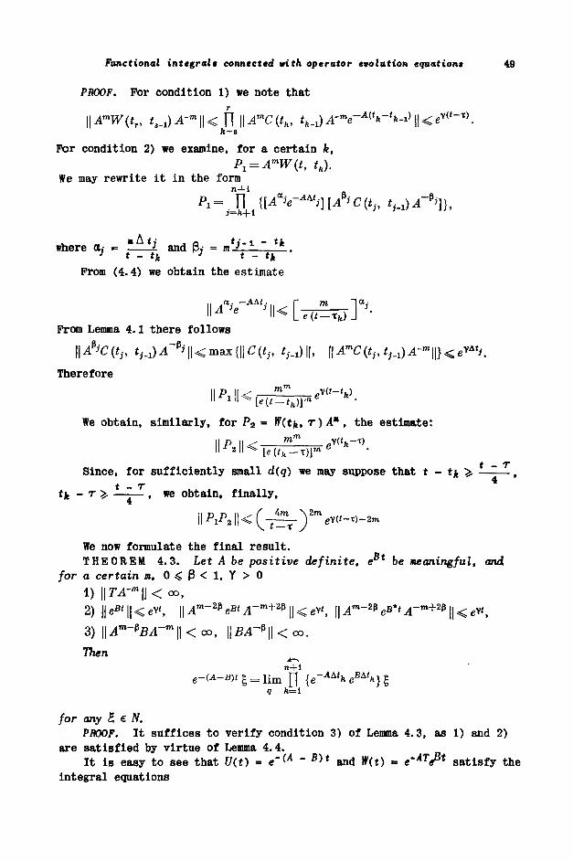
functional integral* connected with operator evolution equation» 49

PROOF. For condition 1) we note that

\\AmW(tT, д А - ц < Р | | Я ( 1 к 1 i f e _ 1 M A ( i ' > v ( ' - o

Рог condition 2) we examine, for a certain k,

P1 = A

mW(t, t

h).

We may rewrite it in the formn+l

Л= .=П %

where a,- = ϊ*±1 and β,· = « 'J ' 1 ~ '*J * - tk

H} t - tk

Prom (4.4) we obtain the estimate

From Lemma 4.1 there follows

\\A*iC(t}, <

м)^-^||<тах

Therefore

I I P I

We obtain, similarly, for P2 = ^(**. т)Д", the estimate:

t 7"Since, for sufficiently small d(q) we may suppose that t - tk Ъ- .

t -τ 4

- τ . , we obtain, finally,

We now formulate the final result.THEOREM 4.3. Let A be positive definite, e be meaningful, and

for a certain m, 0 < ( 3 < 1 , Υ > 01) \\TA-m\\<a>,

2) | | e * ' | | < e v i , H m ~ 2 f J e B i ^ - m + 2 P | | < ev*, | μ " - 2 Ρ β Β * ' Л " т + 2 р | | < ev«,

3) \\Ат-*ВА~т\\ < oo, \\BA-+\\ < oo.

Then

е-<А-в>< ξ = lim Π {e-A"heBAtk}lq k=i

for any S, € N.PROOF. It suffices to verify condition 3) of Lemma 4.3, as 1) and 2)

are satisfied by virtue of Lemma 4.4.It is easy to see that U(t) = e'<A ~ B)t and W(t) = e'^e8* satisfy the

integral equations

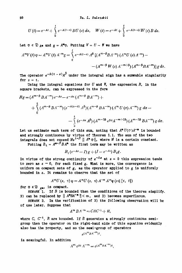
50 Yu. L. Daletskii

t t

U (t) = e~At + \ e-W-V BU (s) ds, W (t) = e~At + J e~A(t~s) w (s) В ds.ο о

Let φ e 3) д« and g = Λ"φ. Putting К = U - № we havet

AmV (t) φ = AmV (<) ""g = \ e-Mt-s) A* [{Am~^BA'm) {AmU (s) A~m) -о

- (Ат~* W (s) Л~

т + Р) (4

т"

р£Л-т)] g ds.

The operator e"'4^* ~

S^A^ under the integral sign has a summable singularity

for s = t.

Using the integral equations for U and W, the expression R, in thesquare brackets, can be expressed in the form

I

Rg = (Л т ~ р BA~m) e~A° - e~As (Am^ BA~m) +

Л т ~ р BA~m) (e~Ms-c) A^) (А т~р Б ^ ~ т ) ( Л т С/ (σ) A~m) g da -

- \ (e-Ό

Let us estimate each term of this sum, noting that A"U(a )A~* is boundedand strongly continuous by virtue of Theorem 1.1. The sum of the twointegrals does not exceed Ms

1'^ \\ Α"φ||, where Μ is a certain constant.

Putting Bi = AM~PBA* the first term may be written as

_ β-A.) Blg.

In virtue of the strong continuity of е"л* at s = 0 this expression tends

to zero as s -» 0, for each fixed g. What is more, the convergence isuniform on compact sets of g, as the operator applied to g is uniformlybounded in s. It remains to observe that the set of

AmU(s, x)<( = A

mU(s, τ) A'

m A

my (s 6 [t, i])

for φ еЗ) Ал, is compact.

REMARK 1. If В is bounded then the conditions of the theorem simplify.3) can be replaced by || А*ВА~

Л \\ < со, and 2) becomes superfluous.

REMARK 2. In the verification of 2) the following observation will beof use later. Suppose that

where С, СГ1, R are bounded. If В generates a strongly continuous semi-

group then the operator on the right-hand side of this equation evidently

also has the property, and so the semi-group of operators

e(A

mBA-

m)t_

is meaningful. In addition

Am e

Bt A~

m =

е

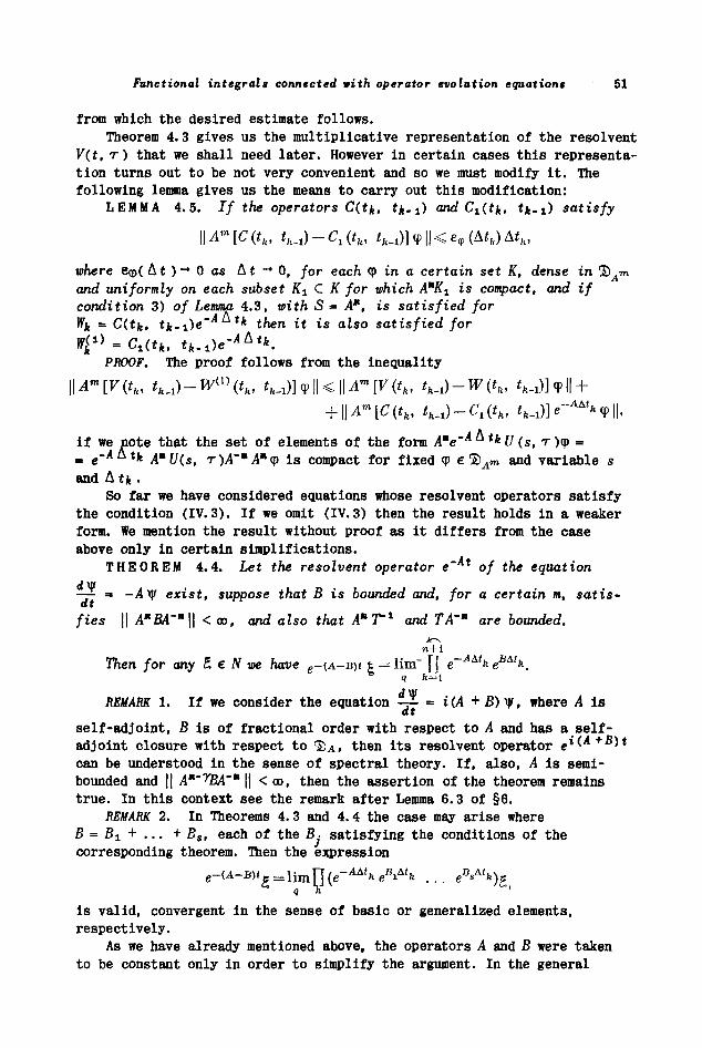
Functional integrals connected vith operator evolution equations 51

from which the desired estimate follows.

Theorem 4.3 gives us the multiplicative representation of the resolvent

V(t, τ ) that we shall need later. However in certain cases this representa-

tion turns out to be not very convenient and so we must modify it. The

following lemma gives us the means to carry out this modification:

L E M M A 4.5. If the operators C(tk. i*-i) and Ci(tk, tjfc-i) satisfy

Um[C(t

k, hJ-C^, ί^ΜφΙΚβ,,ίΔίΛΔ^,

where 8φ(Δί ) -* 0 as At -* 0, for each φ in a certain set K, dense in ®Am

and uniformly on each subset Kj. С К for which АлК

г is compact, and if

condition 3) of Lemma 4.3, with S = A*, is satisfied for

Wfc = C(tk. tk-i)e~A *

k then it is also satisfied forA

PROOF. The proof follows from the inequality

II/4"* ΓF4i t ) W^ (t t )] w II < II Am \V(t t ) Wit t

+ \\Am[C(t

k, hJ-C^, «„_!>] e-^^'* φ ||,

i f we note that the set of elements of the form A*e~ tkU (s, τ ) φ == e-A Δ tk χ» U(s> т )Д-* д * φ i s compact for fixed φ e %Am and var iable s

and Δ tk .So far we have considered equations whose resolvent operators satisfy

the condition (IV.3). If we omit (IV.3) then the result holds in a weaker

form. We mention the result without proof as it differs from the case

above only in certain simplifications.

T H E O R E M 4.4. Let the resolvent operator e" * of the equation

—ϋ- = -.4 ψ exist, suppose that В is bounded and, for a certain m, sat is-dt

fies || АлВА

т*\\ < oo, and also that A^T

1 and ТА'* are bounded.

n+l

Then for any I e N we have e-(A-B)t t = Km" [j e~AAtk e

BAth.q ft=*l

REMARK 1. If we consider the equation ~ = i(A + Β) ψ, where A isdt

self-adjoint, В is of fractional order with respect to A and has a self-

adjoint closure with respect to фА, then its resolvent operator

can be understood in the sense of spectral theory. If, also, A is semi-

bounded and || ΑΛ~

ΎΒΑ~* \\ < со, then the assertion of the theorem remains

true. In this context see the remark after Lemma 6.3 of §6.

REMARK 2. In Theorems 4.3 and 4.4 the case may arise where

В = βχ + ... + B

s, each of the В • satisfying the conditions of the

corresponding theorem. Then the expression

is valid, convergent in the sense of basic or generalized elements,

respectively.

As we have already mentioned above, the operators A and В were taken

to be constant only in order to simplify the argument. In the general

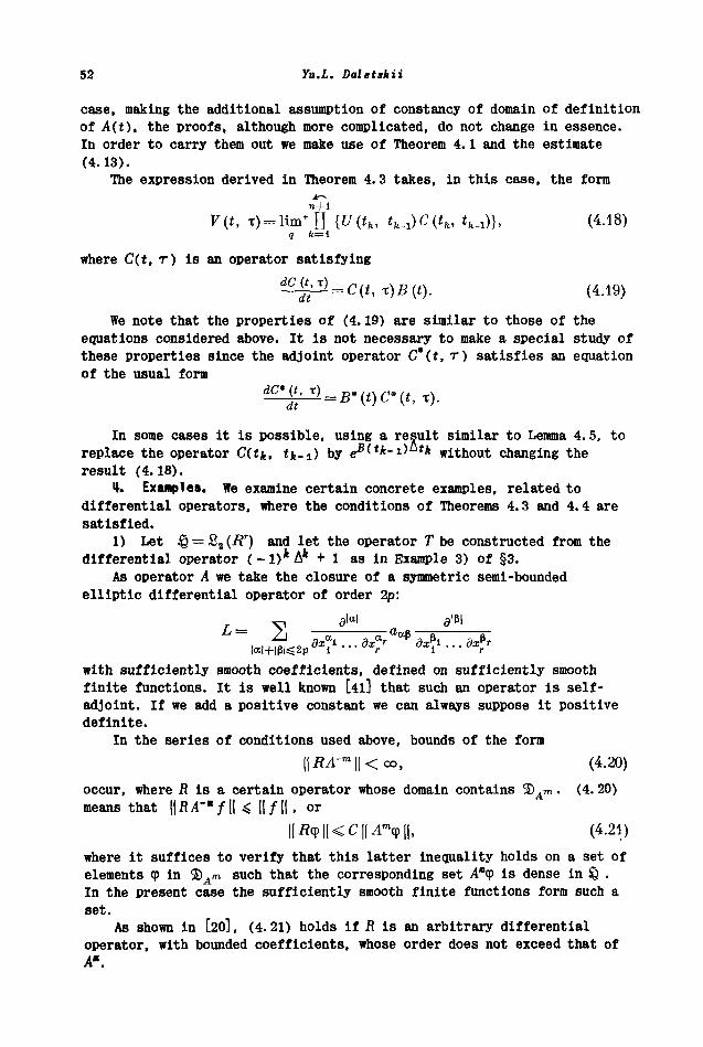
52 Yu.L. Daletskii

case, making the additional assumption of constancy of domain of definitionof A(t), the proofs, although more complicated, do not change in essence.In order to carry them out we make use of Theorem 4.1 and the estimate(4.13).

The expression derived in Theorem 4.3 takes, in this case, the form

n+1

V(t, T) = lim+ Π {U(t

h, t

h^)C(t

k, i

fc_i)}, (4-18)

g fe=l

where C(t, τ ) is an operator satisfying

^fU = C(t,x)B(t). (4.19)

We note that the properties of (4.19) are similar to those of theequations considered above. It is not necessary to make a special study ofthese properties since the adjoint operator C*(t, r ) satisfies an equationof the usual form

^£l^Jl = B*{t)C*(t, τ).

In some cases it is possible, using a result similar to Lemma 4.5, toreplace the operator C(tk, tk-i) by «>*(**-ι>

Δί* without changing the

result (4.18).4. Examples. We examine certain concrete examples, related to

differential operators, where the conditions of Theorems 4.3 and 4.4 aresatisfied.

1) Let i§ = Sa (R

r) and let the operator Τ be constructed from the

differential operator (-1)*Δ* + 1 as in Example 3) of §3.As operator A we take the closure of a symmetric semi-bounded

elliptic differential operator of order 2p:

,

with sufficiently smooth coefficients, defined on sufficiently smoothfinite functions. It is well known [4l] that such an operator is self-adjoint. If we add a positive constant we can always suppose it positivedefinite.

In the series of conditions used above, bounds of the form

||ЛЛ-"Ч|<со, (4.20)

occur, where R is a certain operator whose domain contains ©Λ™ . (4.20)

means that ||ЯЛ""/|| 4 II/II . or|| Дер ||< С || Л > ||, (4.21)

where it suffices to verify that this latter inequality holds on a set ofelements φ in Ъ

Ат such that the corresponding set Α"φ is dense in & .

In the present case the sufficiently smooth finite functions form such aset.

As shown in [20], (4.21) holds if Л is an arbitrary differentialoperator, with bounded coefficients, whose order does not exceed that ofA".

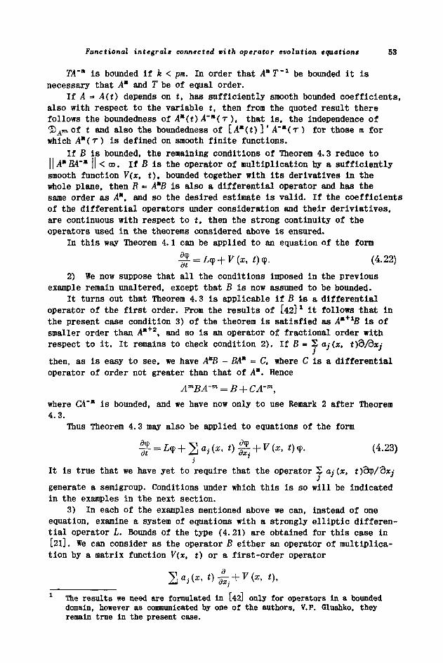
Functional integrals connected vith operator evolution equations 53

TA~m is bounded if k < pm. In order that A T "

1 be bounded it is

necessary that A* and Τ be of equal order.If A = A(t) depends on t, has sufficiently smooth bounded coefficients,

also with respect to the variable t, then from the quoted result therefollows the boundedness of A

M(t) А~

л(т), that is. the independence of

®Am of t and also the boundedness of iA

m(t) ] ' А~

л(т) for those m for

which Α*(τ) is defined on smooth finite functions.

If В is bounded, the remaining conditions of Theorem 4.3 reduce to||Λ"β4"" || < oo. if В is the operator of multiplication by a sufficientlysmooth function V(x, t), bounded together with its derivatives in thewhole plane, then R = A

mB is also a differential operator and has the

same order as Am, and so the desired estimate is valid. If the coefficients

of the differential operators under consideration and their deriviatives,are continuous with respect to t, then the strong continuity of theoperators used in the theorems considered above is ensured.

In this way Theorem 4.1 can be applied to an equation of the form

^- = L<? + V{x, ί)φ. (4.22)

2) We now suppose that all the conditions imposed in the previousexample remain unaltered, except that В is now assumed to be bounded.

It turns out that Theorem 4.3 is applicable if β is a differentialoperator of the first order. Prom the results of [42]* it follows that inthe present case condition 3) of the theorem is satisfied as A

M+iB is of

smaller order than A"+ 2, and so is an operator of fractional order with

respect to it. It remains to check condition 2). If Β = Σ aj(x, t)"d/dxj

then, as is easy to see, we have ΑΛΒ - ВА

Л = С, where С is a differential

operator of order not greater than that of A*. Hence

where G4"" is bounded, and we have now only to use Remark 2 after Theorem4.3.

Thus Theorem 4.3 may also be applied to equations of the form

,{χ, t)^+V(x, ί)φ· (4.23)

It is true that we have yet to require that the operator Σ α,· (χ, ί)9φ/3χ,-J J J

generate a semigroup. Conditions under which this is so will be indicatedin the examples in the next section.

3) In each of the examples mentioned above we can, instead of oneequation, examine a system of equations with a strongly elliptic differen-tial operator L. Bounds of the type (4. 21) are obtained for this case in[2l]. We can consider as the operator В either an operator of multiplica-tion by a matrix function V(x, t) or a first-order operator

The results we need are formulated in [42J only for operators in a boundeddomain, however as communicated by one of the authors, V.P. Glushko, theyremain true in the present case.

54 Yu.L. Daletskii

where ay, V are matrix functions.

We note that we can also examine more general systems of equations,not assuming that L is self-adjoint. The general theory set out above isinapplicable, but we can carry out the development by making use of thebounds of the solutions of such systems obtained in [43].

4) Let us pass now to the case when £> = £., (G) where G is a certainbounded domain of the space R

r. We must now associate certain boundary con-

ditions with each of the differential operators.In order that ||ΤΑ"* || < 00 be satisfied it is necessary that Τ be

independent of the boundary conditions entering into the definition of A".We note however that for m > 1 the boundary conditions associated with thislatter operator depend essentially on A.

In this context we shall examine two cases. Firstly the case m = 1.We may take as Τ the operator (-1)*Δ* + 1 with any self-adjoint boundaryconditions, and as A any symmetric elliptic operator of order not less than2k, with self-adjoint boundary conditions stronger than those defining T.We are able to discuss only operators of order not less than 2k,

On the other hand we can take A" for T, and then it will not benecessary to impose any restriction on the order of A, but the normaliza-tion of the generalized eigen-elements ζ

χ will depend on A.

We must choose the boundary conditions in such a way that the in-equalities required by the conditions of the form (4. 20) are satisfied.Such inequalities are derived in [19], [21], [22].

The condition of the form || Α*ΒΑ~Λι \\ < 00 now imposes certain restric-

tions on В as it must leave invariant the domain of definition of A"1 and

this means, generally speaking, for an operator of the form

2M *)3

that its coefficients must satisfy the given boundary conditions. It

suffices, for example, for the coefficients and their derivatives of

sufficiently high order to vanish on the boundary of G. We note that for

such an operator В the vanishing of the ay(x, t) on the boundary is

necessary in order that В be the generator of a semigroup in G. We shall

discuss this further in the examples examined in the next section. We note

finally that if m = 1, A is considered with zero boundary conditions, and

В reduces to multiplication by the sufficiently smooth function V(x, t),

then it suffices that this function^ be continuous, together with its

derivatives, in the closed domain G, as multiplication by such a function

does not violate the zero boundary conditions.

If A(t) depends on the time we can, by means of Theorem 4.2, examine

the case m = 1, or, if we use Remark 2 after this theorem, the case m = 2.

For щ > 2 the conditions of Theorem 4.2 impose special requirements on

A(t), its coefficients must satisfy certain boundary conditions.

If we take account of these requirements we can apply Theorem 4. 3 to a

mixed boundary value problem for an equation

where L is an elliptic operator. We can also examine systems of a similar

Functional integrals connected vith operator evolution equations 55

type with a strongly elliptic operator L.

In all the examples examined above the resolvent operator of thedifferential equation satisfied the condition (IV. 3). This allowed us toapply Theorem 4.3 and to obtain the multiplicative expression of thegenerating order in the sense of convergence of basic elements.

We now pass to examples where conditions (IV.1, 2), only are satisfied.In this case Theorem 4.4 allows us to obtain the corresponding expansionin the sense of convergence of generalized elements.

5) Let ig=S2(/?

r) We consider an equation of the form

g a} (z, t)^ + V (x, t) ψ, (4.24)

i

where the notation is as in the examples considered above. The functions

aj, V are supposed real. Also the operator on the right-hand side differs

only by a bounded term from an operator of the form iAlt where A

x is self-

adjoint. A similar expansion will also be valid when instead of one equa-

tion we consider a system of equations with symmetric matrices.

In this case we can apply Theorem 4. 4 and the following remark. We

recall that for its application the domains of Τ and A* must coincide.

This means that they must be of the same order.

It will be necessary together with (4.24) to examine an equation

ЩFor e > 0 the properties do not differ from those of the equations

examined in the first examples since the resolvent operator of such anequation satisfies the condition (IV.3).

If we apply Theorems 4.3 and 4.4 we obtain the expansion for theresolvent V(t, τ , ε), convergent, for ε > 0, in the sense of convergenceof basic functions, and for ε = 0 in the sense of convergence of generalizedfunctions.

The special cases of (4.24) are:a) SchrSdinger's equation (with bounded smooth potential)

b) Schrudinger's equation in the presence of electromagnetic forces

•3—•i**+£c) A system of equations of the form

2 V*) Ψ,к =1

where ait σ

2, σ

3 are Pauli spin matrices.

We can also examine an equation of the form (4.24) in a domain С С йг,

taking into account all the requirements imposed in example 3).

56 Yu.L. Daletskii

8) Let us examine in £ 2 (flj.) a hyperbolic system of equations

(4.25)

where a(x) and b(x) are certain bounded, sufficiently smooth matrixfunctions, a(x) being hermitian.

The operator iA on the right-hand side has the property: A differs froma self-adjoint operator by a bounded term. In fact

A* = [-ia(x) — ]*= -i — a(x)= - ia(x) ~-ia'(x) = A-ia'(x),

and so

Im A = —тт.— = a' (x).Δι

Thus the resolvent of (4.25) exists and satisfies the conditions(IV. 1. 2).

For a sufficiently large constant k the operator Ai = A + ki has a

bounded inverse. Since the operator

A\ = - α2 (χ) Λ. -

[a (χ) a' (x) + 2a (x)] ±- - *»

32

has the same domain of definition as -5-1 + 1 we can apply Theorem 4.4

to equation (4.25).Examples of this type will be studied in the next section.

§5. Abstract hyperbolic equations

I. Characteristics of the abstract evolution equation.In this section we shall examine, in an abstract form, a class of

evolution equations whose properties are similar to those of hyperbolicsystems of first order differential equations.

We shall consider, in UQ , a strongly continuous group of operatorse (-00 < t < 00) generating the closed unbounded operator A. This group,as follows from Theorem 4.1, exists if we have the representation

A = AO + A

V (5.1)

where Ao is self-adjoint and A

x is bounded. We shall usually suppose that

such a representation holds.Let us assume also that there is given, in i§, a self-adjoint operator

В with a simple spectrum and spectral set Ε(Δ).We shall later assume that certain additional conditions similar to

(III. 2, 3, 4) are satisfied.(V.1) For each function f(x) in a certain class F there exists a set

®/CZ®/(B) Π ® Α dense in ig, and such that

/ (B) ©/ С Φχ, A% m ®/ ( B )

.

The class F contains at least the piece-wise differentiable functions.(V. 2) If f(x) is continuously differentiable then for Φ e ®л П ®/(В)

Functional integrals connected with operator evolution equations 57

we have f(B)q> e % A .

(V. 3) В has a generating element и (ordinary or improper) belongingto Φ Α . Every element Аи can be represented in the form Аи = g(B)u, whereg(x) is a bounded continuously differentiable function.

We now introduce the following definition.Let the function S(t, x) be given on a certain subset Ш of the real

axis and mapping Ш one-one onto itself for each t. We assume that S(t, x)is continuous in χ for each t, and for each χ has a derivative S'

t(t, x),

which is uniformly bounded in χ for t = 0.

If for each interval Δ

ешЕ (Δ) = Ε (S (t, Δ)) е

ш (5.2)

is true, where Δ4 = S(t, Δ ) is the interval into which S(t, x) maps Δ, then

we shall call the group eiAt hyperbolic with respect to B, and S(t, x) a

characteristic of the group.

Prom equation (5.2) there follows, for any t, r, and Δ,

E(S(t + x, A))e

iA«+V = eiAW>E(A)^eiA*E(S(t, A))eiAt =

= E(S(t, S(x,

from which

S(t + T, A) = S(t, S(x, Δ)) (5.3)to within sets of spectral measure zero.

In particular 5(0, Δ) = Δ and the inverse function of S(t, x) isS(-t, x).

We now examine some consequences of the definition of hyperbolicity.LEMMA 5.1. If ψ e Φ / ( Β ) and eiAt ψ e ®/ ( S(-t, в»' where f(x) is

measurable with respect to the spectral measure, then

eiAtf{B)ty = j(S(-t, B))eiAt^. (5.4)

PROOF. Firstly let f(x) be a bounded continuous function. Prom (5.2)there follows

eiAt Σ f(x

h)E{A

h)$= 2 f(x

h)E(S(t, Δ

Λ))β"'ψ =

fe=l J t = l

= f 1(S(-t, ук))Е(Ь

и)е"*Ъ

where Дд. (k = 1, ..., p) is a finite subdivision of the axis, xk e Δ*. andy

k = S(t, x

k). If we pass to the limit with respect to the various sub-

divisions of the axis we obtain (5.4).

If now f{x) is an arbitrary measurable function for which the integrals

\f{x)\*d(Ex% ψ), J \f(S(-t, χ))\*ά(Ε

χ^

Α%

β"'ψ), (5.5)

—oo —oo

exist, then, considering a sequence of bounded functions fn(x) convergent

to f(x) almost everywhere with respect to the spectral measure, and passing

to the limit in

58 Yu.L. Daletskii

which is permissible by the boundedness of the integrals (5.5) and the

inequality | fn(x) \ <• \ f(x) |, we obtain the desired equation.

Let us substitute the generating element u for ψ in (5.4). Since the

vector function <p(t) = elAtf(B)u, for <p

0 = f(B)u e Ъ

А , satisfies

g-Uq, (5.6)

with the initial value cp0. then knowing the solution of the Cauchy problem

for (5.6) for the condition φ0 = u we obtain the solution of this problem

for a dense set of initial vectors.

If also Аи - 0, then it can be shown that elAtu = u, and for the

solution of the Cauchy problem it then suffices to know the characteristic

S(t. x):q>(O = /(S(-i, B))u. (5.7)

We note that if f(x) vanishes outside the interval Δ, that is, if φ0

belongs to the subspace $3& = Ε (Δ) ig then the vector φ(ί) belongs to the

subspace ^S(-(,A) (displaced subspace). These considerations justify the

definitions we have adopted.

EXAMPLE 1. Let g = £2 (RJ, В be the operator of multiplication by the

variable x, и = 1 being an improper generating element.

We consider the operator

First let h(x) & 0. For the solution of the Cauchy problem for

§Г = *(*)£*. Ψ(0, *) = /(*), (5.8)we must, as is well-known, find the characteristics of the equation (5.8)

fromdx . .

with the condition *(0) = x0. Let us suppose that a set χ = 3(t, x

0) of

these curves exists on a certain interval 0 t ζ Τ, and that the inverse

function x0 - y(t, x) also exists on this interval.

The solution of the problem (5.8) is given by the formula

We note that in the present case Аи = О. Comparing the expression we have

obtained with (5.7) we see that γ(ί, χ) = S(-t, χ), i.e. β(ί, χ) = S(t, χ).

Thus the S(t, x) in the present case coincide with the characteristics

of (5.8).

In order that a set of curves P(t, x) satisfying the conditions formu-

lated above shall exist, it is sufficient, as may easily be deduced from

general theorems on differential equations, that the functions g(x). g' (x)

be uniformly bounded on the real axis. This also follows from example 5)

of the previous chapter.

From the existence of characteristics in (0, T) there follows their

extensibility to an unbounded interval of t since the problem is homogeneous

in t.

Functional integrals connected with operator evolution equations 59

We turn now to the case when h(x) 4 0. Let us assume for simplicity

that g(x) and h(x) are continuous, and g(x) does not vanish. Introducing

the new unknown functionx

•ipj (x, t) = ψ (χ, t) exp \ — p | eta,

we reduce the problem to the previous case, with the condition

Hence

V С *)V С )The function exp \ '-—dx here represents e

i'*

tu, and so the expression

X

we have obtained for the solution corresponds to

eiAl f(B)u = f(S( — t, В)) е

ш и.

EXAMPLE 2. Let us assume that in the equation

g(x) vanishes at the ends of (a, b): g(a) = g(6) = 0, and is different

from zero inside the interval.

The characteristics passing through α and 6 have, in this case, the

equations χ = α, χ = b. Since the characteristics issuing from different

points do not intersect, the values of χ = β(ί, x0) for x

0 e (a, b) also

belong to this interval.

We can therefore examine the given equation in £ 2(a, 6).

The following lemma gives a condition for the group to be hyperbolic.

L E M M A 5.2. Let the condition (V.I) be satisfied and let f(x) belong

to F and have a derivative summable on finite intervals.

Then if φ £©/' (в)П®/> there follows from (5.4) the equation

Ai{B)q-f{B)A4 = iS'(0,B)f{B)4. (5.9)

PROOF. Let f(x) be a bounded function in F with a bounded derivative,and let φ e ©/. Differentiating

eiAt f (Β) φ = / (S ( - 1 , B)) eiAt φwith respect to t we obtain

ieiAt Af {Β) φ = - / ' (S ( - 1 , B))S't(-t, B)eiAt q> + if{S(-t, B)) eiAt Αφ.

If we put t = 0 and recall that 5(0, B) = В then we obtain (5.9).

60 Yu.L. Daletskii

Let us now turn to an arbitrary function f(x) satisfying the conditions

of the lemma and construct a sequence of bounded functions fn(x), with

bounded derivatives, approximating f(x) and its derivative, from below,

almost everywhere. Then (5.9) holds for /„(*) and passing to the limit we

obtain the desired result.

REMARK. If f(x) is bounded and smooth and (V.2) is satisfied, then

(5.9) holds for φ еЪА-

Prom the result just proved we can draw certain conclusions concerning

the structure of the operator A generating the hyperbolic group.

Let us define on the set of elements of the form / = f(B)u, where f(x)

is a smooth finite function, an operator D by means of

Df = iS't(Q,B)f(B)u.

If ψ = ЩВ)и is an element of the same form, then

= iS' (0, B) [f (Β) ψ (В) + / (Β) ψ' (Β)] и-if (В) S' (0, В) ψ' (В) и == iS'iO

Prom this and (5.9) it follows that

and so A - D is a function of В :

Under the isomorphism of £) onto 2 2,σ. Β is transformed into the

operator of multiplication by x, and the operator A, by the last formula,

goes into the operator defined on smooth finite functions by

<t(x)± + h(x) (q>(z) = S('(0, x)),

i.e. a first order differential operator.

Fundamental to the definition of hyperbolicity is (5.2) or its

equivalent (5.4). It is not difficult to see that the same consequences

result from the more general relation

eiAt

f (β) ψ = / (5 (_ i, B)) e ^ + R (/, t) ψ, (5.10)

where it is assumed that P(f, ί)ψ has a derivative which tends to zero as

t -* 0, for smooth functions /(*). In fact after differentiating (5.10) at

t = 0 we again obtain (5.9).

We note that (5.10) does not give any essential generalization by

comparison with (5.4). In fact, using

n+l n+1

" (2 ( Σ Λ )we obtain the formula

- Δ ί1, 5(-Δί,, ..., ά·(-Αί

η.,. Л). ...

£ Ч Ч > . (5.11)

where

Functional integrals connected with operator evolution equations 61

-At1, S(-Attt . . . , S(-Mh_1, B), . . . ))), Ath]eiAtk.

Each of the terms of this sum is, under the given conditions, of orderί^). Let us assume that the quantities

tend uniformly to zero. Then the second term in (5.11) tends to zero as

d(q) - 0, and we obtain (5.4) with (generally speaking) a new function

J(-t, x)= lim 5(-Δίΐ 5 5(-Δί,, ..., 5(-Δί

η + 1, χ), ...)).

d(.q\->0

2. The sufficiency of the conditions of hyperbolicity.

In the previous section it was shown that from the hyperbolicity of the

group β * relative to the operator В it followed that the commutators

Af(B) - f(B)A commute with the functions of B.

Here we consider how far this condition suffices for the hyperbolicity

of the group. We note first that, as will now be shown, this condition can

be weakened to the assumption that only AB - BA commutes with B. As the

latter operator has a simple spectrum we obtain1

AB-BA = i<f(B). (5.12)

If A is self-adjoint then φ(χ), as is easily seen turns out to be real. Weshall always assume that i t is real although A may not be self-adjoint; forexample i t may be the sum of a self-adjoint operator and a function of B.

LEMMA 5.3. Let f(x) have a locally summable derivative. If theconditions (V.I, 2) ore satisfied, then from (5.12) there follows

[Af (B) -f (Β) Α) ψ = if (Β) φ {Β) ψ (5.13)where

Ψ6Φ/'(Β)Φ(Β)Γ)Φ/(Β).

PROOF. Let ψ e ΦΒΦ(Β)· Then

(AB2 - B2A) ψ = (AB - Β Α) Βψ + В (АВ - ΒΑ) ψ = i • 25q> (Β) ψ.

Equation (5.13) is established similarly for the case when f(x) is a poly-

nomial in x, and ψ e Φ/'(Β)Φ(Β)· In particular, in any such domain there are

elements of the form ψ = y(B)u, where ψ is a finite function. Let /(*) also

be a finite function and let fn(x) be a sequence of polynomials approxi-

mating it, and its derivative, uniformly in the interval Δ, outside which

f{x) and ψ(*) vanish. Consider the equation

Ε (Δ) Afn (Β) ψ - Ε (Δ) /

η (В) АЦ = iE (Δ) f

n(B) φ (Β) ψ.

In the second and third terms we may pass to the limit, as η -.со. Conse-quently the f irst term also has a limit. Going to the limit, next, asΔ -. (~oo,oo), we obtain (5.13) for the finite functions fix), ψ(*). Further,i t i s easy to drop the condition of finiteness on ψ(*), by approximatingthis function ψ(*), at any element ψ= y(B)u in ©/ЧВ)Ф(В) from below by asequence of smooth finite functions converging almost everywhere.1 Remark added in proof. In the special case Ф(х) = 1 this equation has been

extensively studied (cf. [47]. [4β], [49]).

62 Yu.L. Daletskii

Finally let /(*) be any function as described in the conditions of the

lemma, and let ψ e ф/'(в)Ф(в>- Let us approximate it, together with its

derivative, from below by a sequence of finite smooth functionsfnM (n = 1, 2, ...) convergent almost everywhere. Then ψ e Φ/'<Β)φ(Β)and so

[Afn (B) - f

n(B) Α] ψ = if

n (Β) φ (Β) ψ.

Suppose, also, that ψ e Фдв)· Then we may pass to the limit in the secondand third terms of this equation. Consequently we may also pass to thelimit in the first term. This establishes the lemma.

In the development of the possibilities of the condition (V. 3) it isuseful not to be restricted to the usual generating elements but to usethe improper ones. Let us verify in this context that we can define A onsuch elements. As shown in §3.4 it suffices to prove the followingassertion.

L E M M A 5.4. Let A be a self-adjoint operator satisfying the condi-tion (5.13). If (V. 2) is satisfied then for any pair of intervals Δ С A

lt

and φ € © л . we have

PROOF. Let Уд (дс) be a continuous differentiable function equal to onefor ж e Δ and to zero for χ e Δι. (5.13) implies

4 ψΔ (Β) - ψ

Δ (Β) Α = ίψ

Δ (Β) ψ (Β).

Multiplying this on the left, tennwise, by £(Δ), and noting that for

x e Δ, \|/д (χ) = 1 and ψ д (χ) = 0, we obtain

Ε (A) A^ (В) = Ε (Α) Α.

Now let / e фА and g e ΦΑΕ(Δ>. We also have Щ(B)f е ф л and so

(ΨΔ(£)/, AE(A)g) = (E(A)AyA(B)f, g) = (E(A)Af, g).

Passing to the limit, so that \уд(х) tends from below to the character-

istic function хд (x) of Δ1 ( we obtain

(AE(A)g,E(A1)f)^(g,E(A)Af),

from which follows, for / e фл:

Ф and Ε (A) A: E(A)AE(A1).

REMARK. It is easy to see that the lemma remains true if A is of the

form (5.1).

Now let us examine how to reconstruct the group of operators eiAt,

hyperbolic with respect to β. Comparing (5.9) and (5.13) we see that if

such a group exists then

<p(x) = S't(0, x).

Thus we must first construct the function S(t, x) satisfying the

conditions

1) 5(0, x) = x,

2) S't(0, ζ) = φ(ζ),

3) S(t + T, X) = S(T, S(t, x)).

Functional integrals connected vith operator evolution equation* 63

If we differentiate the last relation with respect to τ and put τ = 0

we obtain for S(t, x) the differential equation

, χ)). (5.14)

On the other hand, if for each χ in a certain set 9Л, containing the

spectrum of β, there exists in the interval 0 4. t 4 t0, not depending on

x, a unique solution of this equation satisfying the condition 1) then it

also satisfies 2) and 3).

We examine only the case when 5Щ coincides with the whole axis. Prom

general theorems of the theory of differential equations it is not diffi-

cult to conclude that a solution of (5.14), having the properties we

require, exists, at all events, if φ(χ) and its derivative are uniformly

bounded on the axis. Since (5.14) is invariant with respect to time the

solution will exist for all t.

When S(t, x) is found, the group elAt is easily recovered if a

generating element ц (usual or improper), such that Ли = 0, exists.

In fact we also have eiAtu = u, and so

-t, B))u.

It is natural, therefore, to examine the set of operators Tt defined by

Ttf = f{S(-t,B))u for f = f(B)u.

If f{x) is continuously differentiable then the vector-valued function

ψ(ΐ) = Ttf is differentiable with respect to t; moreover from Аи = О and

(5.13) there follows

dTtf

dt ί=0- i , B))S'

t(-t,

(5.15)

Further, by the property 3) we have

Tt+tf = f{S(-t-x, B))u = f(S{-t, S(-x, B)))u = T

xf(S(-t, B)) = T

xT

tf.

Differentiating with respect to τ and putting τ = 0 we obtain, using (5.15),

. (5.16)

(V. 4) Let us assume that the closure of A on the set of elements of

the form ψ(β)ίΐ, where ψ(*) is continuously differentiable, coincides with

A. Then if we know in advance that the group elAt exists,

_^ в)) и. (5.17)

Prom the construction itself it is clear that the group satisfies the

condition (5.4).

Let us now turn to the case wh«n Аи 4 0 but (V.3) is satisfied, that is

xAn = g(B)u, where g(*) is a bounded continuously differentiable function.

In this case

where Axu = 0.

64 Yu.L. Daletskii

As in the demonstration of Theorem 4.3 we can show that

eiAt

= eg(B) t

eiA

lt + /?(£), (5.18)

moreover the operator R(t) is subject to the estimate \\R(t)f || > teAt),

where ε At) -* 0, when / e®A . uniformly on a set of elements / for which

the set [Af } is compact.

It follows from (5.17) and (5.18) that

eiAtf (Β) -ψ = eeWeUitf (B)^ + R (t) f (Β) ψ =

= f(S(-t,

There results a situation similar to that encountered in (5.10). Besides,

in the present case we know in advance that the function S(t, x) has the

property S(t + r, x) = S(t, S(r, x)).

Therefore

f(S(-Atlt S(-At

t, . .., S(-M

h,x), ...))) = f(S(-t

k, x)).

The set of elements of the form Af(S(-tk. β))ψ= <P(ife) for fixed

ψ б Ф А and /(*), and t* varying in [θ, t], is compact, as for a continuous-ly differentiable function f(x) the element φ(ί) is differentiable and hence

also continuous in t. Therefore we can obtain a uniform estimate for the

remainder /^(Οψ reducing, as was shown at the end of the previous section,

to

eiAtf (B)\p = f(S(-t, B)) e

iAi ψ.

Let us formulate the result we have obtained as a theorem.

T H E O R E M 5.1. Let the operator A, of the form (5.1), and the

operator В satisfy the conditions (V.I, 2). Then for the group e to behyperbolic relative to В it is necessary, and if (V.3, 4) are satisfied,sufficient that (5.12) hold, where φ(χ), together with its derivative, isuniformly bounded for χ e (-00,00).

REMARK 1. It is not difficult to deduce from (5.18) that

еш = e^

B· <yV

;.

t

where #, (x, t)= \ g (S (— τ, χ)) dr. Thus in the present case we have

5

eiAtf (В) и = egi(ii· °/ (S ( - t, В)) и. (5.19)

REMARK 2. We could examine the case when the set 9Ji does not coincidewith the whole axis. It is then necessary that the spectrum of В lie in Ю?and, in addition, that for each t, S(t, x) leave Щ invariant. As shown inexample 2 of the previous section, S(t, x) leaves (a, b) invariant ifφ(α) = φ(6) = 0. Thus if the spectrum of В lies in [a, 6] all the resultsstated above remain valid.

REMARK 3. If above we do not assume the existence of the group elAt

then we may try to recover it by using the formulae (5.17) and (5.18).There first arises the question whether the expression

Functional integrals connected with operator evolution equations 65

defines a linear operator. Sinceoo oo

\\Tty(B)u\\*= J \y(S(-t,x))\*da(x)= $ |ψ(*)|«Λτ(5(ί, χ))—CO — OO

and

J—oo

we must have an inequality of the form

Such an inequality holds if, for example, the measure o(S(t, x)) isabsolutely continuous with respect to σ(χ) for sufficiently small t and

da (S (t, x))

dx

If a(x) is the Lebesgue measure then the condition described is satisfiedwhen q>(*) and φ'(*) are uniformly bounded.

In this context we have the interesting question under what circum-stances the spectral function of the operator В is absolutely continuouswith respect to the Lebesgue measure. It is possible that this followsfrom (5.12) under certain additional assumptions (for example, if we sup-pose φ(χ) > 0).

3. A hyperbolic group with a number of characteristics greater thanone.

We now turn to an examination of the case when the operator В has amultiple spectrum. In this case there exist orthogonal projectorsPi, .... Р

л which commute with B:

rn

P,Pk = b

ikPi, Р<В = ВР: (i, A=l, ...m), У,Рь = 1.

We shall say that the group e*^* is hyperbolic if there exist functionsSk(t, x) (k = 1, ..., m) having the properties possessed by the functionS(t, x) of Section 2, and for which

e^f (Β) Λ Ψ = / [Sh (-1, B)] e"'i>

hib + R

h (/, *) ψ, (5.20).

where the quantity Rk(f, *)Ψ tends to zero as t — 0 if ψ e 5)A and f(x) iscontinuously differentiable. We assume also that Ρ*ψ e Φ Α if ψ e Φ

Λ·

We shall call the functions S*(*· x) (k = I m) characteristics.As simple examples show, the equations (5.20), do not imply similar

equations with i?*(/, *) = °. in contrast to the case m = 1.Differentiating (5.20) and putting t = 0 we obtain

(Ar=l, ...,m), (5.21).

where Фь(я) = S'b (0, x) is a necessary condition for hyperbolicity.

" t

ββ Yu.L. Daletskii

We shall show below that, as in the case m = 1, with additional hypo-theses this condition is found to be sufficient for e to be hyperbolic.

We first consider an example.

Let a(x), g(x) be matrix functions, and let a(x) be symmetric. Considerthe system of first order differential equations

Let pi(x), pz(x). .... Pm(x) be matrices with project onto the eigen-vectors of the matrix a(x), so that

where λ*(χ) (feel, .... m) are eigenvalues of a(x). We suppose that thematrix functions Pk(x) are differentiable with respect to x. This is so if,for example, a(x) is differentiable and the multiplicities of its eigen-values do not vary with x. We shall denote by Pk the operator ofmultiplication by the matrix pk(x) and we verify that for the operators

iA = a(x)g- + g(x) and Pfc the conditions (5.21) are satisfied.

In fact, if f(x) is a scalar function

iAPkf(x) = a(x)~-*-'- + g{a

= f(x)a (χ) - ^ \- f {x) a (x) P)l (x) +• g (/) ph (x) j (u)

and on the other hand

if {x) APh = f(x)a (x) ^ + / (x) g (x) Ph (x),

from which i t follows that

APkf (B)~ f (B) APk = if (B)lk(B) Pk ( f t = l , . . . , m).

Let us now consider the sufficiency of the conditions (5.21). Weexamine first a special case, and suppose that A commutes with theP

k (k = 1 m):

Condition (5.21) can be written in the form

AJ (Bh) - / {B

h) A

k = icp

fe (B

k) f (B

h),

where Afe = PfeA, Bfe = Рф are operators in the subspace ^к = Р^. In this

subspace B^ has a simple spectrum and so we may apply the arguments of

Sections 1 and 2.

Consequently, under the hypotheses adopted in those sections, the

group elAftt

satisfies the condition (5.13), which can also be written

Moreover the group β is completely defined by the functions * ( ) ,the operator B, and the values of e

%At on a system of generating elements.

We now turn to the case when A is an arbitrary operator satisfying(5.21). Prom this condition it follows that

Functional integrals connected with operator evolution equations 67

Thus iA can be represented as the sum of two operators

the first of which, iAx = ιSP^APfc commutes with each Pk (k = 1, ..., m)

and the second, Ci = i Σ Pi AP^ commutes with B.

Let us suppose that C± is bounded. Then in virtue of (5.21) we may

deduce from the formula

analogous to (5.18), which also holds in the present case, the following

equation, for a continuously differentiable function f(x),

e^f (B) Pk4> - e^e^itf (Β) i>fc<p + R1=*f [Sk (t, B)]

= f [Sk (t, B)} e^'Ph<p - / [Sh (t, B)} tfa + Rv

which means that the group β is hyperbolic, and has characteristics

coinciding with those of the group eiAlt.

Finally we note that the group elAt can be recovered from the group

e ** already constructed, by means of the formula

n+1

eiAi = lim Π (e

c*%

tAiA'k), (5.22)

q ft=l

which follows from Theorem 4.4 with Τ = I and m = 0.

Thus we have

T H E O R E M 5.2. Under the conditions of Theorem 5.1, for the group

β to be hyperbolic relative to the operator B, with spectrum of

multiplicity m, it is necessary that the conditions (5.21) be satisfied.

If the operators PiAPk (i 4 k) are bounded, and (V.3, 4) are satisfied,

then those conditions are sufficient.

We can show, similarly to the case when В has a simple spectrum, that

if the conditions (5.21) are satisfied, the equation θψ/θί = ΐΛψ does not

differ, up to an isomorphism, from the equation referred to in the example

considered above in the space 2™,a·

The theory may be extended, without alteration, to the case when in-

stead of functions of one operator В we consider functions of the

commuting set of operators Blt .... B

r. The characteristics will in this

case be functions in the space Лг.

As an example we can take a system of the form

with commuting matrices α^(χ), in particular one equation of this form.

4. The triangular case.

We examine in detail a special case where the formula (5.22) takes a

more transparent form.

Let us suppose that the condition

68 Yu.L. Daletskii

PjAP^O (j>k). (5.23)

is satisfied. Then we shall say that A is triangular with respect to B.

It is not difficult to verify that in this case

In fact, let φ e %A then for η > k we have

*Ζέ£ΐ* φ = iPne™Pk<f = i Σ РпЛР,-ешР^ = iPnAPnPn

з

The vector φ(ί) = PnelAtP№ satisfying this equation vanishes for t = 0

and so, by the uniqueness theorem, vanishes identically. Similarly we mayprove that P

n-ie

iAtPk4> = 0. and so on.

Let us now turn to the representation (5.22) and write it in the form

eiAt _ u m 2 2 · · · 2 Pje

Q j j ΐ ^ Κ ~ Α * S - 2

. . . Pjec^4iAiMiPj . (5.24)

It is clear that the indices must here satisfy the condition

/ s < / s - l < · • · < / < > .

since

and for jk > jkwl PjkeC Pjk-i· w h l c n l s Proved as for the operator e l A t .We note now that

i-P,- (5-25)

In fact

since PjCPk = 0 for j > k and Pke

CtPj for j < k.

It follows from (5.25) that if, in any term in (5.24), we meet a groupof factors of the form

Ρ e

C A ' f t e i A i A i 'JU " β — ι "R—a τ — χ

with equal suffixes jk = j f e _ ± = . . . = j r . 1 , then it reduces to the

operator Pj,heiAl (tk — tT^).

Prom this it follows that we can write (5.24) in the form

* " · = . Σ . h Σ Η Ρ

where the suffixes form a strictly decreasing sequence.

Finally we note that by the equation

•±PfP,№+...

functional integrals connected with operator evolution equations 69

and the strong continuity of e*'*1* at zero, we have the relation

P.eCMeiA^tps = PfPsAt + о (At).

Passing to the limit in (5.24) as d(q) — 0 we can omit the term ο(Δΐ),the sums over the suffixes fej become integrals, and we obtain the repre-sentation

еш = 2 2 \ d t A dtn-i · • • \ dhe^-tn) РьСРь^ Xn = 0 in, • • · . 30 0 0 °

x 6ίΑλ(ΐη-ΐη-ι)ρ.ηι0Ρ^2. . .PhCPkeiAih. (5.26)

As an example let us examine the one-dimensional wave equation

We may write it as a system

dt dx "·" "a»

~dT~ ~~dx ·

Here

I1 °lll ^ - I |

O 1I ! Ρ -II

1 °ll » no оoo · ** о

t-t)j •

The formula (5.26) takes the formt

fiiAt —— g i A j i _i

II о

which is equivalent, as is easy to see, to the well-known formula of

D' Alembert.

6. Fundamental solutions of evolution equations

I. Abstract parabolic equations.

Let us examine the differential equation

= [A(t) + B(t)]y (6.1)

in Й . assuming that its resolvent operator U(t, r) has the properties(IV.1, 2). We suppose also that, for a certain m 1, the operatorsTA'

m(t), A

m(t)U(t, τ), U(t, τ)Α*(τ), (t > τ) are bounded.

Then the condition (IV.3) is satisfied. As follows from Lemma 3.3there exist operators 0(t, τ), 0*(t, r) mapping N continuously into ® .

Consider the vector-valued function

Рог t > τ i t s values are basic elements. Since for t > s > τ

70 Yu.L. DaletMkii

where ψ, = U(s, τ)ψ0 e Ф

А™

(,) С ®

Α(β) , and on elements of Φ

Α(») . U(t, s)

is strongly differentiable and satisfies

then ψ(ί) is the solution of (6.1) for t > r, and its values belong t o ®Am

We now examine the behaviour of this function as t ->τ. For φ € © wehave

(ψ (t), φ) = φ (t. χ) Ι, φ) = (ξ, U* (t, χ) φ).

If φ e ©Am

( i ) then this last expression tends to (£, φ). In fact for £ e Q

this is so since U(t, r)£ -· S as t -»τ, in the sense of convergence in & .Since & is dense in N it remains to show that the vectors U*(t, τ)φ areuniformly bounded in Φ . But this is so since

\\U*(t,x)if\i=\\TU*(t,x)cf\\<\\TA-m(r)\\.\\A

m(r)U*(t,x)A-

m(t)\\-\\A

m(t)<p\\.

Thus, in ΦΑ»*

(ί) which in general is contained in Φ , we have

lim(i|>(i), φ) = (|, φ),ί-*τ

implying the convergence of ψ(ί) to the initial element 5 in a weakersense, it is true, than weak convergence in N.

If A*(t)T~i is bounded then %.т„. = ф and we have weak convergence

in ЛГ.These arguments show that it is natural to consider

as the solution of (6.1) with the generalized initial element S.Now let 1 5* i (x € 83 ) be a complete set of generalized elements in N.

We recall that this means that any basic element Φ can be represented asan integral

φ-$(φ, U i , da(x). (6.2)58

weakly convergent in N.

The set of vector-valued functions

*x(*) = U(t,x)l

x (*6 93) (6.3)

will be called the set of fundamental solutions of (6.1) corresponding tothe given complete set {5

Ж! of generalized elements.

Let us show that any solution of (6.1) having a basic element Φ asinitial value can be expressed as an integral of fundamental solutions.

In fact since U(t, τ) is continuous from N to Φ if we apply it term byterm to (6.2) we obtain

U(t,x) = U(t,s)U(s,x).

where for t > т the integral converges in the sense of weak convergenceof basic elements.

Functional integrals connected with operator evolution equations 71

EXAMPLE. The resolvent operator ofm

§ = Ш+% ah (x, t) ·#- + V (*, t) ψ, (6.4)ft=l

as discussed in the examples of §4, where L is a self-adjoint ellipticoperator considered on the whole space R

m or in a certain domain.

Prom the arguments above there follows the existence of fundamentalsolutions of (6.4), reducing to the delta-function 6(x - x

0) for t = 0. It

is found, also, that for t > 0 these solutions are basic elements, i.e.they belong to a certain space of the type if|. In the case of a boundeddomain G the fundamental solutions we have obtained are found to be smoothin the closed domain G, for t > 0, and to satisfy the boundary conditionsassociated with A", as their values belong to the domain ®

Am.

In the case of equations in the whole space Rm the existence of

fundamental solutions was shown by S.D. Eidel'man for much more generalequations than (6.4) [43].

Instead of one equation (6.4) we can examine a system of equations witha strongly elliptic operator L.

We remark that we imposed the requirement of self-adjointness on L inorder to simplify the discussion. We could, using the results of [β], [ll],[12], weaken this condition and so obtain the existence of fundamentalsolutions for a wider class of equations. It would be of interest to in-vestigate how far the usual results can be obtained in this way, and to tryto study the properties of fundamental solutions by abstract methods.

For the mapping of $& into S2, a studied in §3, the function

4>* (0 -* (Ψ* С). У = {U (t, τ) lx, l

v) = S (x, t; x, y)

which is the kernel corresponding to the operator U(t, τ), corresponds tothe fundamental solution of the equation (β.1).

L E M M A 6.1. If \&x\ is a complete system of generalized eigen-

elements of a spectral set of operators Ε(Δ) (Δ С Rr) and satisfies the

conditions (III.1, 2), and the equation (6.1) satisfies the conditions(IV.1, 2, 3), then its fundamental solution generates the kernel(fundamental kernel)

which we can take as transition function for the construction of a condi-tional quasi-measure [i*.

PROOF. For t > s > τ we have

U(t,x) = U(t,8)U(s,x).

As was shown in §3, operators are multiplied by convolution of theirkernels and so equation (2.5):

S (t, t; x, y)-= \S (τ, s; x, z) S (x, t; z, y) da (z)

holds.The kernel S(r, t; x, y), as a function of the argument x, and also y,

belongs to Й2, a for t > τ.

72 Yu.L. Daletskii

If T "1 is a Hilbert-Schmidt operator then S has summable square with

respect to the pair (x. y). In fact in this case the operator

U(t, τ) = T~lrIV(t, τ) is also a Hilbert-Schmidt operator, and it suffices

to use Lemma 3.3.

If Γ "1 is not a Hilbert-Schmidt operator but Τ~

1Ε(Δ) is, for any

finite Δ, and also the set of basic elements Ф л which Ε(Δ) maps into

basic elements is dense in !& , then the assertion of Lemma 3.3 remains true

for U(t, r)E(h), and so the kernel corresponding to it is square-integrable

with respect to (x, y). This means that S(T. t; x, y) (r < t) is square-

integrable in a domain in which one of the variables varies between finite

limits, and the other between infinite limits.

This establishes the lemma.

Рог the construction of the quasi-measure μ8 it is still necessary to

satisfy the condition (2.6). we mention certain conditions under which

this is so. Рог simplicity we formulate the result for the case A = const.,

В = const.

L E M M A 6.2. Let there exist a sequence φη € © such that

Лр„ = ( -A + Β)φη e Φ , the sequences of functions Ф

п(ж) = (Φη·δ*) and

Ψη(*) = № m £χ) are uniformly bounded, and ψ

η(χ) -* 1, Ψ

η(χ) -· 0 oZmost

everywhere with respect to o(x), as η -»οο. 77ien if

{ | S (t, t; x, y) | da (y) < oo for t > τ we have

33

^ S(τ, t; x, y)da{y) = \.

•ё

PROOF. Since

t

б φη

= = ψ

η ~\" \ с H(D

n ds

t

о

we may write, for t > 0,t

= (φη> 1я) +б

As η -»со the second term tends to zero. In fact (Щ>п, £

у) - 0 and the

function {lv, [e

Hs]* l

x) is summable. This means that

Also, since Щп е ф , it follows that this expression is uniformly bounded

with respect to s, and therefore the outer integral tends to zero.

Thus, for η -oo, (ея*Фп» £

ж) - 1. On the other hand

(6Η'φ

η) ξ

χ) = (φ

η, [^']*S«)= Ι (Φη. l

v){e

Httv,

and we may pass to the limit under the integral sign on the right-hand side,

Functional integrals connected with operator evolution equations 73

and obtain the expression above. This establishes the lemma.

REMARK. An elliptic differential operator L containing no undifferenti-

ated terms satisfies the conditions of the lemma. Hence the integral over

the whole space of the fundamental solution of the parabolic equation

Э w-57 = Ζ,ψ, with such an operator, is equal to one.

Let us examine again equation (6.1) and the equation

Theorem 4.3 enables us to express the resolvent operator of the first ofthem by means of the resolvent of the second. Prom the representation (4.18)we obtained there, using the rule of composition for the product of opera-tors, we obtain a formula for the representation of the kernel correspond-ing to the fundamental solution of equation (6.1):

(U (t, τ) lx, Ιυ) = Hm [ ... \G (τ, 1ц χ, at,) G (tv t2; хл, хг) ...

•G (tn, t; xn, y) da (xj ...da (xn), (6.6)

where

G(x,t;x,y) = (V(t,T)C(t,T)lx,ly). (6.7)

We note that, along with (6.6), an equation differing only in the

order of the operators V and С in (6.7) is also true. The proof does not

differ from the derivation of (6.6).

In the following section we shall derive from those relations the

formulae expressing the fundamental solution of (6.1) by a functional

integral with respect to the conditional quasi-measure μ£ associated withequation (6.5).

2. Generalized fundamental solutions.

We now examine equation (6.1), assuming that its resolvent operatorsatisfies the conditions (IV.1, 2), but does not satisfy (IV.3).

If we suppose that ТА* and A'mT are bounded, then from (IV. 2) we

deduce the boundedness of the operator

747(i, x)T~\

In view of Lemma 3.2 there exists in N the operator 0*(t, τ).In this way we see that TU*(t, τ)Τ~

ι is bounded, and so 0(t, τ) exists,

acting in N.The generalized element

will be called, by analogy with the case examined earlier, a fundamentalsolution of (6.1).

It follows from

<P= \ (Φ- ξ.)!* da (χ)&

that the solution of this equation, with the basic initial element φ, is

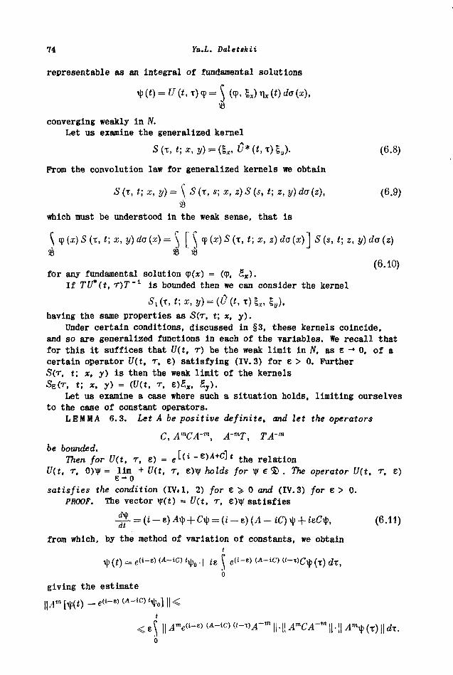
74 Yu.L. Daletskii

representable as an integral of fundamental solutions

ψ (ί) = U (ί, τ) φ = ξ (φ, ξχ) η

χ (ί) dff (χ),

S3

converging weakly in Ν.Let us examine the generalized kernel

S{T,t;x,y) = (tx,C*(t,x)l

y). (6.8)

Prom the convolution law for generalized kernels we obtain

S (τ, f; χ, y)=[s (τ, β; χ, ζ) S (s, ί; ζ, y) da (z), (6.9)

83which must be understood in the weak sense, that is

\<?{x)S ( τ , t; x , y)da{x)=\> [ ^ φ (χ) S(x,t; χ , ζ) da ( * ) ] 5 ( ί , t; ζ, у) da {z)

S3 S3 S3

(6.10)for any fundamental solution φ(χ) = (φ, Ζχ).

If TU*(t, r)Tml is bounded then we can consider the kernel

5, (τ, f;x, y) = (U (t, χ) ξχ, |

y) ,

having the same properties as S(T, t; я, у).Under certain conditions, discussed in §3, these kernels coincide,

and so are generalized functions in each of the variables. We recall that

for this it suffices that U(t, τ) be the weak limit in N, as ε - 0, of acertain operator i/(t, т, е) satisfying (IV.3) for ε > 0. FurtherS(T, t; x, y) is then the weak limit of the kernelsS

E( T , t; x, y) = (i/(t, τ, z)Z

x, £

y).

Let us examine a case where such a situation holds, limiting ourselvesto the case of constant operators.

L E M M A 6.3. Let A be positive definite, and let the operators

C, AmCA-m, A~mT,be bounded. r

Then for U{t, τ, ε) = e L ( i - e M + c J * the r e l a t i o n

U(t, τ, 0)ψ = lim + U(t, τ, ε)ψ holds for ψ € Φ . The operator U(t, τ, ε)ε - ο

satisfies the condition (IV·1, 2) for ε > 0 and (IV.3) for ε > 0.PROOF. The vector \)/(t) = U(t, τ, ε)ψ satisf ies

- ^ = (i - β) 4ψ + CI|J = (i - ε) (4 - iC) ψ + ieCiJ), (6.11)

from which, by the method of variation of constants, we obtain

t

ψ (t) =•• е^-^ <A-

ic> 'ψ

0 -f it \ e^-

8) <

A-

iC> C-^CIJJ (τ) dx,

bgiving the estimate

t

Ό

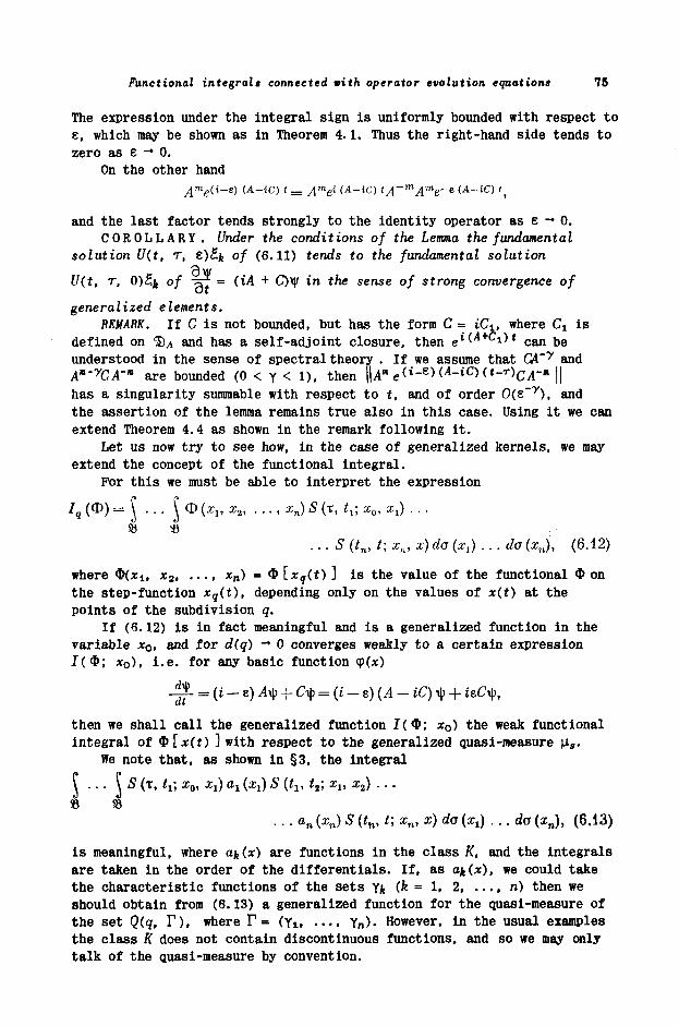
Functional integrals connected with operator evolution equation» 75

The expression under the integral sign is uniformly bounded with respect to

ε, which may be shown as in Theorem 4.1. Thus the right-hand side tends to

zero as ε -* 0.

On the other hand

and the last factor tends strongly to the identity operator as ε -* 0.C O R O L L A R Y . Under the conditions of the Lemma the fundamental

solution U(t, τ, 8)£fc of (6.11) tends to the fundamental solution

U(t, τ, 0)5fc of "o~ = (ίΑ + φ ψ in the sense of strong convergence of

generalized elements.

REMARK. If С is not bounded, but has the form С = iCit where Ci is

defined on ЪА and has a self-adjoint closure, then

e

i^A+Cl^t can be

understood in the sense of spectral theory . If we assume that CA'y and

A*-y

CA-» are bounded (0 < γ < 1), then \\A*

β<*-

ε)Μ-*Ο (t-r)

CA-m ||

has a singularity summable with respect to t, and of order O(e~r), and

the assertion of the lemma remains true also in this case. Using it we can

extend Theorem 4.4 as shown in the remark following it.

Let us now try to see how, in the case of generalized kernels, we may

extend the concept of the functional integral.

For this we must be able to interpret the expression

Iq (Φ) == J ... J Φ (x

v x

tl ..., x

n) S (τ, i

i; x

0, Xl) . . .

Ь SB

... S (tn, t; x

n, x) da (x,) ...da (x

n), (6.12)

where Ф(хи x

2 x

n) = Φ [x

q(t) ] is the value of the functional Φ on

the step-function xq(t), depending only on the values of x(t) at the

points of the subdivision q.

It (6.12) is in fact meaningful and is a generalized function in the

variable x0, and for d(q) -* 0 converges weakly to a certain expression

ί(Φ; *o). i-e. for any basic function

-i$- = (i - ε) Aty + С-ф = (ί - ε) (Α - iC) ψ + ieC\p,i

then we shall call the generalized function Ι(Φ; χ0) the weak functional

integral of Φ[*(ί) ] with respect to the generalized quasi-measure μβ.

We note that, as shown in §3, the integral

S (τ, V. x0, Xy) a

t (xj) S (t

lt t

2; x

lt x

2) ...

... an {x

n) S (i

n, t; x

n, x) da (xj ...da (x

n), (6.13)

is meaningful, where а^(х) are functions in the class K, and the integralsare taken in the order of the differentials. If, as α*(χ), we could takethe characteristic functions of the sets γ^ (k = 1, 2, ..., n) then weshould obtain from (6.13) a generalized function for the quasi-measure of

the set Q(q, Γ ) , where Γ = (Yt γ

η) . However, in the usual examples

the class К does not contain discontinuous functions, and so we may onlytalk of the quasi-measure by convention.

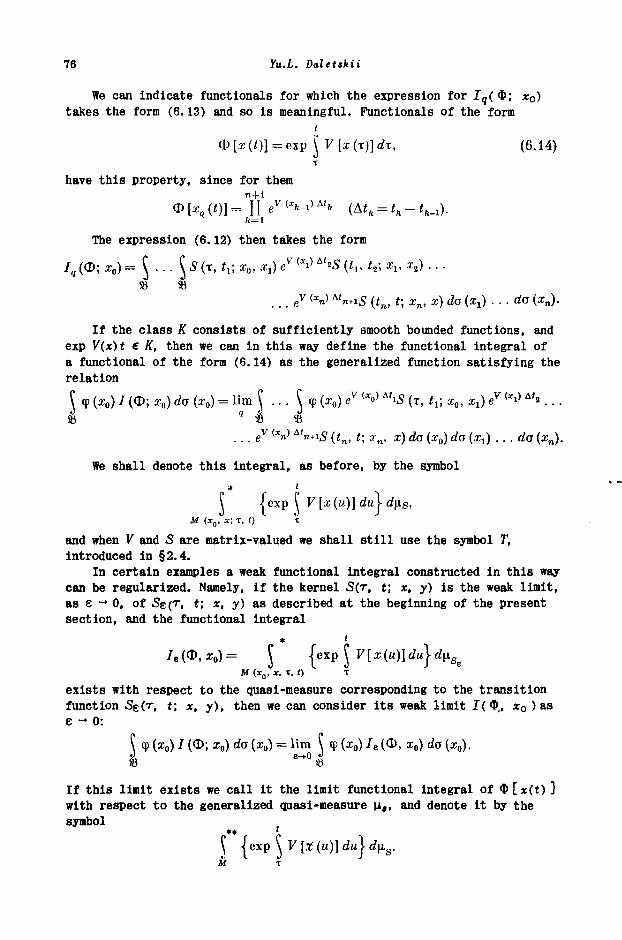
76 Yu.L. Daletskii

We can indicate functionals for which the expression for 1д( Ф ; х

0)

takes the form (6.13) and so is meaningful. Functionals of the form

t

Φ [χ (t)] = exp jj V [χ (τ)] dx, (6.14)τ

have this property, since for themn+i

Φ Κ (0] = Д eV ('*-ι>

Δ'* (At

h = t

h- t^).

The expression (6.12) then takes the form

Iq (Φ; x

0) = \ . . . \ S (τ, t

x; x

0, Xj) e

v (Xl) &'2S (i

l5 t

2; x

v x

2) . . .

SB Я. ..

e

v <*n>

Δ ί»

+ι5 (f

n, ί; x

n, χ) da (х

г) . - . da (x

n).

If the class К consists of sufficiently smooth bounded functions, and

exp V(x)t e K, then we can in this way define the functional integral of

a functional of the form (6.14) as the generalized function satisfying the

relation

\ φ {x0) Ι (Φ; x

0) da (x

0) = U m \ ... \ψ (x

0) e

v (lo>

&liS (τ, t

x; x

0, х

г) e

v ^

ΔΙ» . . .

« Q

S3 аз

. . . e

y (3Cn'

Δίη+ι5' (t

n, t; x

n, x) da (x

0) da (х

г) .. . da (x

n).

We shall denote this integral, as before, by the symbol

-{exp \ V[x(u)]du\ άμβ,L .) J

τand when V and θ are matrix-valued we shall still use the symbol T,introduced in §2.4.

In certain examples a weak functional integral constructed in this waycan be regularized. Namely, if the kernel S(r, t; x, y) is the weak limit,as ε - Ό , of Se(T, t; x, y) as described at the beginning of the presentsection, and the functional integral

/е(Ф, x

o) = \ -{exp \ F [ X ( H ) ] C

Μ (χ0> χ, t. 0 X

exists with respect to the quasi-measure corresponding to the transitionfunction 5g(T, t; x, y), then we can consider its weak limit Ι(Φ,, χ

0 ) as

ε - 0:

\ ψ (x0) / (Φ; x

0) da (x

0) = lira \ φ (x

0) /

ε (Φ, x

0) da (x

0).

If this limit exists we call it the limit functional integral of Φ [ * ( Ο ]with respect to the generalized quasi-measure μ,, and denote it by thesymbol

Μ

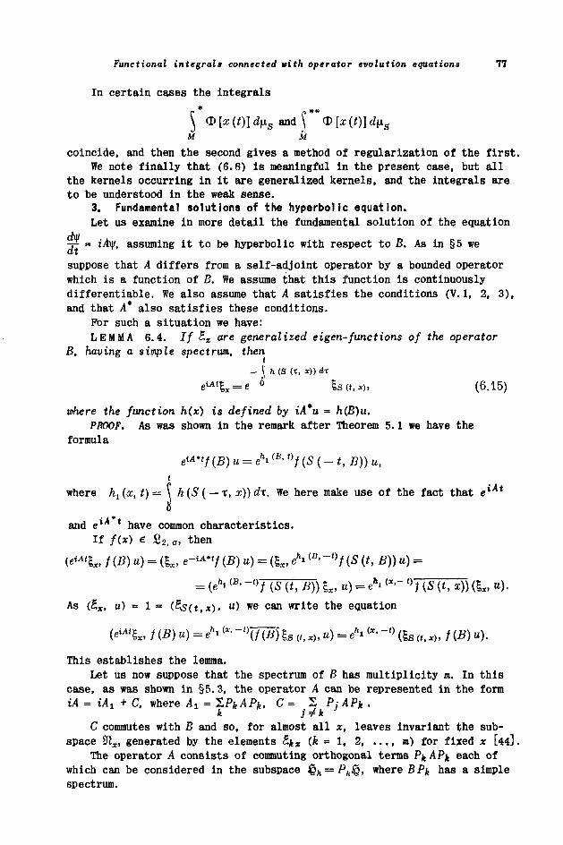
Functional integrals connected with operator evolution equations 77

In certain cases the integrals

5 ^Μ Μ

coincide, and then the second gives a method of regularization of the first.We note finally that (6.6) is meaningful in the present case, but all

the kernels occurring in it are generalized kernels, and the integrals areto be understood in the weak sense.

3. Fundamental solutions of the hyperbolic equation.Let us examine in more detail the fundamental solution of the equation

τ-*- = ιΑψ, assuming it to be hyperbolic with respect to B. As in §5 we

suppose that A differs from a self-adjoint operator by a bounded operatorwhich is a function of B. We assume that this function is continuouslydifferentiable. We also assume that A satisfies the conditions (V.I, 2, 3),and that A* also satisfies these conditions.

For such a situation we have:LEMMA 6.4. If Ζχ are generalized ei gen-fund ions of the operator

B, having a simple spectrum, then

- J h(S (t, *)) dx

eiA% = e ° tsu.x), (6.15)

where the function h(x) is defined by iA*u = h(B)u.PROOF. As was shown in the remark after Theorem 5.1 we have the

formula

eiA''f {В) и = Л

( B > f)/ (S (- t, В)) и,

t

where hx (x, t) — \ k(S( — T, x))dx. We here make use of the fact that e

lAt

and eiA * have common characteristics.

If f{x) e S2 ; σ, then

(e^lx, f (B) u) = (l

x, tr"4f (B) u) = (l

x, eh

(B> ~'>/ (5 (t, В)) и) =

= (e"!(B· -'>/ (S (t, B)) l

x, u) = e*i <*•-

l)i(S(t,x)) β

χ, и).

As (£ж, и) = 1 = (&S(t,x)· ") we can write the equation

(e"%, f (B) u) = Л <*' -ЧЩЩ ξ8 „, „, и) = eh <*· "<> fo

(t> x), f (B) u).

This establishes the lemma.

Let us now suppose that the spectrum of В has multiplicity m. In this

case, as was shown in §5.3, the operator A can be represented in the formiA = iAi + C, where A{ = SPjfe/lPjfe, С = Σ Pj APk .

Λ J к

С commutes with В and so, for almost all x, leaves invariant the sub-

space %lx, generated by the elements £** (k = 1, 2 m) for fixed χ [44].

The operator A consists of commuting orthogonal terms P* ДР* each ofwhich can be considered in the subspace ^

h — P

h^, where BPk has a simple

spectrum.

78 Yu.L. Daletskii

Let us suppose t h a t the elements ть 0 = 1 , . . . . m) forming a base in3ix. are chosen so t h a t

Л-Чк* =* bih4h*- (6.16)Then

m

ft—1 J

where

and the function hyix) is defined by iPj A*PJU = hj(B)u.

Suppose now that the generalized eigen-elements S,jx of the operator В

do not satisfy the condition (6.16). We shall suppose that they are

related to the f\kx by the formulae

η,χ = 2 »ki (*) lkx> tjx = Σ v»kj (*) Лих.h ft

where the matrices v(x) and w = v"1 are continuously differentiable with

respect to x. Prom (6.17) we then obtain the relation

= 2 2 whj (x) β"** <'•*> u r b ( 5 h (i, *)) ξ, (Sk (t, x)). (6.18)

We shall, later, need the value of this expression when we discard

terms of order o(t).Putting φ*(χ) = Sk(O, x) we write the equations

i

hlh(i, x) = \ К(S

h(t, x))dx = h

k(x)t + o(t),

Ό

Vkr (Sh (t, X)) = V

hr (x) + V'

kr (X) ф

Ь (X)t + O (t).

Replacing Лц5./

4 жч by Ή ^ + φ , / ^ , and, in the term containing the factor

t, by the element r\kx, we obtain

1X г, ь '

r h

+ 1 2 u>hj (x) е~1Нъ (JC) ФЙ (*) v'rk (x) Irx + ω . (6.19)r, ft

where the expression ω is irrelevant for the calculations connected with

(β.β), in certain cases, as we shall see in the next chapter.

7. Functional integrals associated with abstract parabolic equations

I. Functional integrals with a scalar quasi-measure.

After the preparatory work of the previous chapters we can now obtain

Yu.L. Daletikii 79

the theorems on the representation of solutions of differential equationsof various types in the form of functional integrals.

In this section we shall examine equations of the form

d±=-A(t)$ + Bm, (7.1)

whose resolvent operator V(t, τ) satisfies the conditions (IV. 1, 2, 3). Inconcrete applications there correspond to these equations differentialequations, or systems of parabolic type, and in this context we employ thename: abstract parabolic equations.

Let us assume that the coefficients in (7.1) satisfy the conditions ofTheorem 4.3, so that the kernel corresponding to its fundamental solutionis representable in the form

n+l

W{x, t;x,y) = (V(t,x)lx,l

v) = l i m { . . . U l [

p

(7.2)where

G (tk.u t

h; x

h.

lf x

h) = (U (t

k.lt t

h) С (<

h.lf t

h) k

fc_

if Ц ) . (7.3)

We examine first the case when the operators are constant, i.e.

U(t, τ) = «-•*<«-*>, C{t, t) = «»<«-*>, V(t, τ) = e<-*+« <«-τ>.

We shall, for the time being, suppose that В is bounded. Let us assume

that it can be represented in the form

(x)dEx, (7.4)

where £(Δ) is a certain simple spectral set of operators satisfying (III.1)(Δ С R

m). There exists in N a complete system {£

x \ (x e R

m) for which

only if there exists in φ a dense subset φ' such that

Taking in (7.3) this complete system of generalized elements we obtain

G (t, t; x, y) = ef W <'-0 (e~^ <«-Ό lx, l

y). (7.5)

Let us write 5(r, t; x, у) = (е-

А<*-

г)£х, S

y) and substitute (7.5) in

(7.2). We obtain the representation

e-(A-B)iE t )

=

SJCI Чу) —

n+l n+l

4 Rm Rm "ft=O " / i = l

+

f (Ч-ι) At h\ Ц S (i

ft_lt t

h; x

h_

v x

k) da (χ^.,.άσ (χ

η)=

9 R?

n+l

, dx), (7.6)

where \is(4· ^) ^ s t h e quasi-measure generated by the transition function

80 Yu.L. Daletskii

S(T. f, x, y).

Now let us consider in the space M(x, y; 0, t) the functional

t

Φ[ζ(τ)] = βχρ f(x(x))dx. (7.7)

6

The corresponding functional Фд ίχ(τ) ] has the formi

Фд [χ (ί)] = Ф[х, (t)} = exp \ f (xq (τ)) dx =ό

n+l 'ft n+1

= e x p ^ \ j (xq (τ)) dt = exp ^ 1(хк.х)Мк,h = l i h j fe=l

as *g(i) = x(tfe.i) = xfe.j. for tfc-i < t < tfc.This expression coincides with the integrand in (7.6), and so

{e-(A-B) t

Ιχι l y ) ([

Q

Prom this there follows at once

T H E O R E M 7.1. Let the operator A and the bounded operator В satisfy

the conditions of Theorem 4.3, and let B= \ f(x)dEx, where

RmE(L·) (Δ С fl

M) is a simple spectral set satisfying (III.l).

Then the fundamental solution of -τ-- = -Λψ + βψ, constructed with

respect to the system {&x\ of generalized eigen-elements of the given

spectral set, can be represented as the functional integral

5 { \ ) (7.6')Μ (χ,'ν; 0, ί) Ь

with respect to the quasi-measure [is, generated by the fundamental solutions

solutions of -£ = -Λψ.

REMARK 1. It is not difficult to verify that, assuming

G(x,t;x,y) = (C(t,x)U(t,x)tx,%

l),

we obtain in the finite integral in (7.6) the expression

( Σ /(fc+i) („•!

fe=0

This expression can be regarded as the value Φ[*9(ί)] of the functional

(7.7) if in the definition of xq(t) we change the normalization at the

points of discontinuity and take it to be continuous on the left and noton the right, as we have done so far. We see thus that such a change ofnormalization in the definition of the functional integral turns out tobe unnecessary for functionals of the form (7.7).

We shall see later that this is not always so.Let us turn now to the case when the operators

Functional integrals connected with operator evolution equations 81

A(t), £(*)=$ i(t,x)dEx

depend on t. We assume, as is clear from the notation, that all theoperators B(t) are functions of one and the same spectral set E

x having a

complete system of generalized eigen-elements B,x.

The arguments in this case differ only slightly from those describedabove. In the expression (7.2) we now have U(t, τ) as the resolventoperator of

and C(t, τ) satisfies the equation

Since all the operators f(t, B) commute it is clear that

С {t, т) = ехр \ f(u, B)du

X

and consequentlyt

G(x, t; x, y) = exp j \ f{u, x)du\ S (τ, t; x, y).τ

The formula (7.6) now takes the form

η 'ft + l

(v (<. τ) L· ly) = l i m \ Θ Χ Ρ | Σ ^ i{u,xk)du\\Lv

s{q,dx).' «S, - * = 0 'ft

It is clear in this case that the right-hand side represents a functionalintegral of the form

Μ (χ, у; τ, <)

(η,χ(ιι))άιι}άμΙ. (7.8)

The operators B(t) were assumed to commute in order to simplify theargument. If we abandon that hypothesis and suppose that in

B(t)= J }(t,x)dEx(t)

Rm

the spectral set also depends on t then it will be necessary to considera system £

xXt) depending on t.

Рог the transition function we shall take the definition

The other kernels we consider are changed similarly. We can show that after

these changes the formula (7.8) still remains true.

EXAMPLE 1. The conditions of the theorem are satisfied, as is shown

in the examples of §4, by the equation

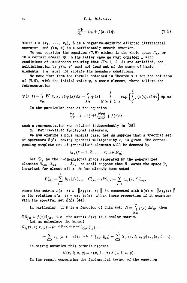
82 Yu.L. Daletskii

|£ = Z4+ /(*,*) ψ, (7.9)

where χ = (л^ хя), L is a negative-definite elliptic differential

operator, and f(x, t) is a sufficiently smooth function.We can consider the equation (7.9) either in the whole space R

a, or

in a certain domain ($. In the latter case we must consider L withconditions of smoothness ensuring that (IV.1, 2, 3) are satisfied, andmultiplication by f(x, t) must not lead out of the space of basicelements, i.e. must not violate the boundary conditions.

We note that from the formula obtained in Theorem 7.1 for the solutionof (7.9), with the initial value φ, a basic element, there follows therepresentation

(x,t)= ξ W(t,x, y)y{x)dx= ^ ^Rm Hm Μ (χ, у, О, О

In the particular case of the equation

such a representation was obtained independently in [35].2. Matrix-valued functional integrals.We now examine a more general case. Let us suppose that a spectral set

of operators £(Δ), having spectral multiplicity r, is given. The corres-ponding complete set of generalized elements will be denoted by

Let Шх be the r-dimensional space generated by the generalized

elements ζίχ, S,

ix, ..., £

г ж. We shall suppose that В leaves the space %l

x

invariant for almost all x. As has already been noted

r r

B IJ X= 2 Κ (

χ) t**>

ch * =

e B%

x= Σ %• <*. *) ,

fe=i k=l

where the matrix c(x, t) = \\cjk(x. t) II is connected with b(x) = ||bjk(x)

by the relation c(x, i) = exp tb(x). В has these properties if it commuteswith the spectral set Ε(Δ) [44].

In particular, if β is a function of this set: B= \ f(x)dEx, then

Rm

В £j x = f(x)B,jx, i .e . the matrix b(x) is a scalar matrix.Let us calculate the kernel

GW(T, t; X, y) = (C- Α(ί-τ,βΒ(ί-τ)ξ.Λΐ ξ.^ =

= Σ ckj (χ, t - τ) (e-A C-T) lhx, | 1 И ) = Σ Slk (τ, t; χ, у) chj (χ, t - τ).

In matrix notation this formula becomes

G (τ, t; x,y) = c (x, t — x)S (τ, t; x, y).

In the result concerning the fundamental kernel of the equation

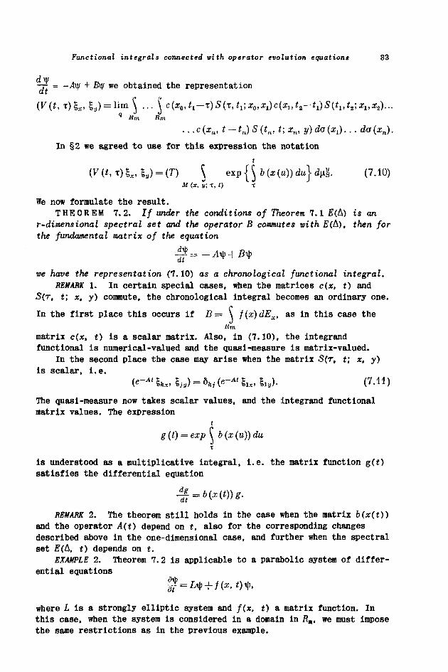
Functional integrals connected with operator evolution equations 83

•— = -Λψ + βψ we obtained the representation

, x)tx, gy) = li

. . . с (аг„, t-tn)S(tn,t;xn, у) da ( x t ) . . . da (х„).

In §2 we agreed to use for this expression the notation

i

(V(ttx)lx,lu) = (T) [ exp{$ δ (*(»)) du}^g. (7.10)Μ (χ, у; τ, Ο τ

We now formulate the result.T H E O R E M 7.2. J/ under the conditions of Theorem 7.1 Ε(Δ) is an

r-dimensional spectral set and the operator В commutes with £(Δ), then forthe fundamental matrix of the equation

we have the representation (7.10) as a chronological functional integral.REMARK 1. In certain special cases, when the matrices c(x, t) and

S(T, t; x, y) commute, the chronological integral becomes an ordinary one.

In the first place this occurs if B= \ f(x)dEx, as in this case the

Яти

matrix c(x, t) is a scalar matrix. Also, in (7.10), the integrandfunctional is numerical-valued and the quasi-measure is matrix-valued.

In the second place the case may arise when the matrix S(r, t; x, y)is scalar, i.e.

(e-*4kx, l

jv) = i>

kj(e-^l

lx, l

lu). (7.11)

The quasi-measure now takes scalar values, and the integrand functionalmatrix values. The expression

g (<) = exp \b(x (u)) du

is understood as a multiplicative integral, i.e. the matrix function g(t)

satisfies the differential equation

REMARK 2. The theorem still holds in the case when the matrix b(x(t))and the operator A(t) depend on t, also for the corresponding changesdescribed above in the one-dimensional case, and further when the spectralset 2?(Δ, t) depends on t.

EXAMPLE 2. Theorem 7.2 is applicable to a parabolic system of differ-ential equations

where L is a strongly elliptic system and f(x, t) a matrix function. Inthis case, when the system is considered in a domain in R

m, we must impose

the same restrictions as in the previous example.

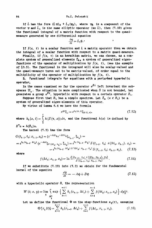
84 Yu.L. Daletskii

If L has the form (ί,ψ)* + Z-i(Wjfe). where ψ* is a component of thevector ψ and L

x is the same elliptic operator (as L). then (7.10) gives

the functional integral of a matrix function with respect to the quasi-measure generated by one differential equation

If f(x, t) is a scalar function and L a matrix operator then we obtainthe integral of a scalar function with respect to a matrix quasi-measure.

Finally, if f(x, t) is an hermitian matrix, we can choose, as a com-plete system of generalized elements Zkx a system of generalized eigen-functions of the operator of multiplication by f(x, t), (see the exampleof §3.5). The functional in the integrand will also be scalar-valued andthe quasi-measure turns out to be matrix-valued, of order equal to themultiplicity of the operator of multiplication by f(x, t).

3. Functional integrals for equations with a perturbed hyperbolicoperator.

In the cases examined so far the operator eBt left invariant the sub-

spaces 9ία. The situation is more complicated when В is not bounded, but

generates a group eBt, hyperbolic with respect to a certain operator B

±.

Suppose first that Bj. has a simple spectrum. Let £x (x e R

x) be a

system of generalized eigen-elements of this operator.By virtue of Lemma 6.4 we have the formula

£S ( l i i e )

, (7.12)t

where ^(x, t) = \ h(S(τ, x))dx, and the functional h(x) is defined byо

B*uо

The kernel (7.3) has the form

_ ehi (хк_ г мк) (е~АА%8 ( A ( f e > Xk)t lXk) = e

h l (xh-v Ath1 S (tk_lf tk; s (Ath, xh_x), xh) =

where

/ (A<h; sk_ l f xft) = I n ^ ^ ΰ , , ΐ ! , ! ^ ' . ^ ) ' ^ · (7·14>

If we substitute (7.13) into (7.2) we obtain for the fundamentalkernel of the equation

(7.15)

with a hyperbolic operator β, the representationn+1 n+1

W (t; χ, у) = lim \ exp •! ^ j " i \xk-^ Ath) + 2J f ( ft' хь-1' xk) f

1

Let us define the functional Φ on the step-functions xq(t), assumingn+i , n+1

Φ Κ (01= Σ M**-i. Δ ί * ) + Σ f(btk,xk_ltxk). (7.16)

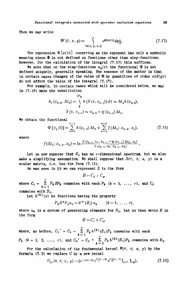
Functional integrals connected vith operator evolution equations 85

Then we may write

W(t;x,y) = ^ ефМ'>]фУ. (7.17)

М(х,"у: O.i)

The expression Φ [x(t)J occurring as the exponent has only a symbolicmeaning since Φ is not defined on functions other than step-functions.However, for the calculation of the integral (7.17) this suffices.

We note that on the step-functions xq(t) the functional Φ is not

defined uniquely, generally speaking. The essence of the matter is thatin certain cases changes of the value of Φ by quantities of order o(d(q))do not affect the value of the integral (7.17).

For example, in certain cases which will be considered below, we mayin (7.16) make the substitution

Ath

ht (ж

й_!, Δί^) = \ h(S (X, aVi)) dx =% At

kk {x

h^,

о

We obtain the functionaln+l л+1

[x (t)\ — 2_ п \хк-\,

fe=l

where

Let us now suppose that Bx has an г-dimensional spectrum, but we also

make a simplifying assumption. We shall suppose that S(r, t; x, y) is ascalar matrix, i.e. has the form (7.11).

As was seen in §5 we can represent В in the form

гwhere C^ = Σ PkBPk commutes with each Pk (k = 1 r), and C

2

commutes with Β χ.

Let h^ (χ) be functions having the property

where щ is a system of generating elements for Bj,. Let us then write В inthe form

where, as before, ( V = CV - Σ P^h^ (Bi)Pfc commutes with each

Pk (k = 1, 2 r). and C

2' = C

2 + Σ P

kh^

k)(BjPk commutes with B

t.

For the calculation of the fundamental kernel W(r, t; x, y) by the

formula (7.2) we replace G by a new kernel

Gn{x,t- x, y) = (e-M'-Ve

cilt-*e

ci(l-x)tjt, l

lV), (7.19)

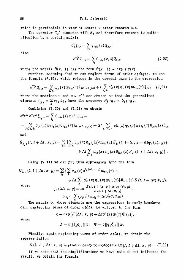
86 Yu.L. Daletskii

which is permissible in view of Remark 2 after Theorem 4.4.

The operator C2' commutes with Βχ and therefore reduces to multi-

plication by a certain matrix

^aEii* = 2- Укк \

x) %>hx''

h

also

e^'S^^W*, t)ihx, (7.20)

where the matrix θ(χ, t) has the form θ(χ, t) = exp ίγ(χ).

Further, assuming that we can neglect terms of order o(d(q)), we use

the formula (6.19), which reduces in the present case to the expression

ec'i

l l

hx = Σ Щи (

x) whh i

x) li*+t<p

k(x) +1 Σ vk (x) <?

h (x) w

hh (x) l

ix, (7.21)

where the matrices ν and w = v'1 are chosen so that the generalized

elements η. = Συ^· Zkx have the property Pj r\k

x = 6j

Combining (7.20) and (7.21) we obtain

gCyAt gC^At £ _ ;;_- \ ft - - (χ*\ pC\Al £ . -—-bj χ ^ . 323l \ / Ь32-)с

— ΔΛ vik \X) wh]2 \ ι "3231 \Χ) bix+ At<(h(x) "Τ L*1 Zj vih \χ) фй \χ) ^йзг У > "nil \х) •32. »·

and

G , (ί, ί + Δί; ж, у) = 2 ( 2 fift (x) 9j23i ( x) «зг (x) Su (t, t+At; χ + At<ph (x),1 32 i. ft

At 2. Vik(x) φ^ (X) Ojan ( ) ύί (

(ί, ί + Δί; a;, y)j .

i, fe

Using (7.11) we can put this expression into the form

Gu , (t, t + Δί; χ, у) = 2 {2 v

lh (χ) e

f^'-·

χ· » w

hk (χ) +

h ft

+ Δί 2 v'sk (χ) φ,, (χ) оду, («)}Λ

ίώ (χ) 5 (ί, ί + Δί; χ, у),

/h (Δί, ж, у) - in sit,t + bt;x,y) ·

The matrix p, whose elements are the expressions in curly brackets,

can, neglecting terms of order ο(Δί), be written in the form

t; x, y) + Atv'(x)w{x)O(x)},

where^ = »||/

ke

ifc||a;, Φ = ν \\<f

h6

jh || w.

Finally, again neglecting terms of order o(At), we obtain the

representation

G(t, t + At; x, y) eFw,

x. v)+At[v'(x)w(x)<i>(x)+y(x)l s (t, t + At; x, y). (7.22)

If we note that the simplifications we have made do not influence the

result, we obtain the formula

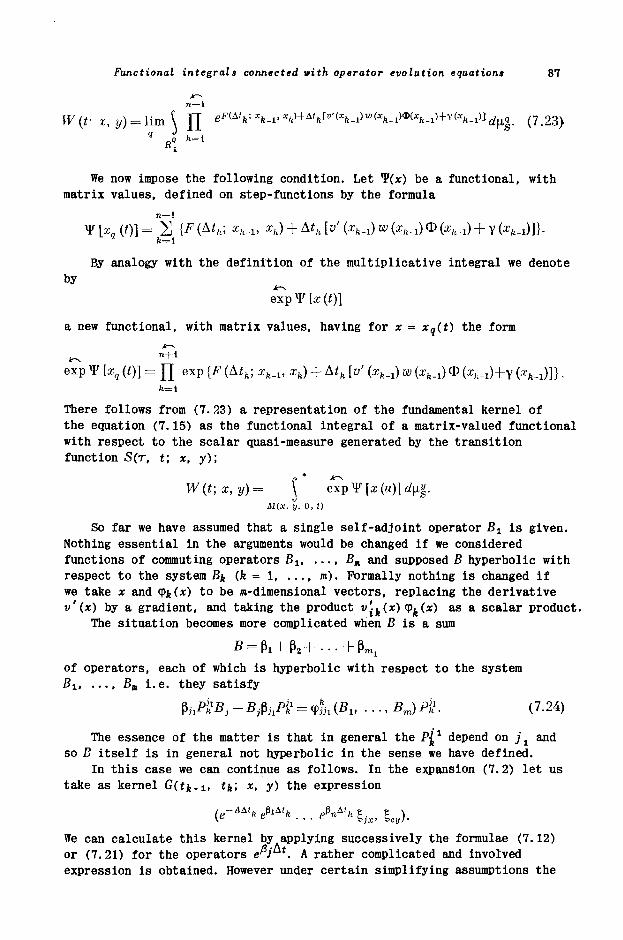
Functional integrals connected with operator evolution equations 87

>->n+1

W{f x, y) = lim\ Π ^ V ' k . i . ^ + i ' k l ' V i ) · ' ^ . ^ - ^ ^ ^ . (7.23)

JWe now impose the following condition. Let Ψ(χ) be a functional, with

matrix values, defined on step-functions by the formula

n+i

Ψ[χ,(ί)]= Σ {F(&h; *k-i. Xk) + tohW(xk-i)u>{Xk-i)<S>(x

k-i) + y(Xk-J]}-

ft=l

By analogy with the definition of the multiplicative integral we denote

by ^

exp Ψ [χ (f)]

a new functional, with matrix values, having for χ = xq(t) the form

exp Ψ [xq (f)] = Π exp {/· (Δί

Λ; x

fe_x, x

h) + At

h [υ' (x^) w (x^) Φ (x

k.t)+y (х

к.г)]}.

There follows from (7.23) a representation of the fundamental kernel ofthe equation (7.15) as the functional integral of a matrix-valued functionalwith respect to the scalar quasi-measure generated by the transitionfunction S(r, t; x, y);

W(t;x,y)= \ е"хр Ψ [χ (α)} άμν.

М(х. у. 0,0

So far we have assumed that a single self-adjoint operator Вг is given.

Nothing essential in the arguments would be changed if we consideredfunctions of commuting operators B

x B

m and supposed В hyperbolic with

respect to the system Bk (k - 1, .... m). Formally nothing is changed ifwe take χ and <Pfe(x) to be m-dimensional vectors, replacing the derivativev'(x) by a gradient, and taking the product v'

ik(x) q>

k(x) as a scalar product.

The situation becomes more complicated when В is a sum

of operators, each of which is hyperbolic with respect to the systemBlt .... B

m i.e. they satisfy

ϊήΡΪΒ,-Β^Ρί^ΨΗΛΒν ...,Вт)Р{К (7.24)

The essence of the matter is that in general the Pj^1 depend on j

ί and

so В itself is in general not hyperbolic in the sense we have defined.In this case we can continue as follows. In the expansion (7.2) let us

take as kernel G(tk-i, tk', x, y) the expression

We can calculate this kernel by applying successively the formulae (7.12)or (7.21) for the operators ew . A rather complicated and involvedexpression is obtained. However under certain simplifying assumptions the

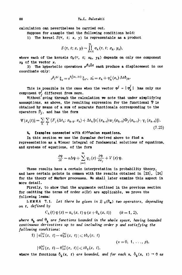
88 Yu.L. Daletskii

calculation can nevertheless be carried out.Suppose for example that the following conditions hold:1) The kernel S(r, t; x, y) is representable as a product

m

S(x, t;x, y)= Π ah(x, t; x

h,y

h),

ft=l

where each of the kernels Ok(τ, t; xk, у к) depends on only one componentхь of the vector x.

2) The hyperbolic operators eP l each produce a displacement in one

coordinate only:

ΛΔ ί l

x = e

hl{x·Δί) , xk = x

h + Ψί Ы Δίδίν

This is .possible in the case when the vector φ^ = {<Pj[ ! has only onecomponent φ

1, different from zero.

Without going through the calculation we note that under simplifyingassumptions, as above, the resulting expression for the functional Ψ isobtained by means of a sum of separate functionals corresponding to theoperators $j, and has the form

[ , ( ) ] Σ Σ ^ * i 4 ) J

4 jJ

к j

(7.25)Ц. Examples connected with diffusion equations.In this section we use the formulae derived above to find a

representation as a Wiener integral of fundamental solutions of equations,and systems of equations, of the form

d

3 = 1

These results have a certain interpretation in probability theory,and have certain points in common with the results obtained in [23], [24]for the theory of Markov processes. We shall later examine this aspect inmore detail.

Firstly, to show that the arguments outlined in the previous sectionfor omitting the terms of order ο(Δί) are applicable, we prove thefollowing lemma:

L E M M A 7.1. Let there be given in 2 2( 1») two operators, dependingon t, defined by

Ch(t)<p(x) = a

k(x,t)<

f(z + e

ll(x,t)) (Λ = 1, 2),

where &k and Q

k are functions bounded in the whole space, having bounded

continuous derivatives up to and including order ρ and satisfying thefollowing conditions:

1) \a№(x, «)-(i(2VJ(x, ί)Ι<*δι(*. Ο

(v = 0, 1, ..., p),

|9(Й(ж, t)-B%(x, t)\

<t6,(x, t),

where the functions 6fe(x, t) are bounded, and for each χ, δ^(χ, t) — 0 as

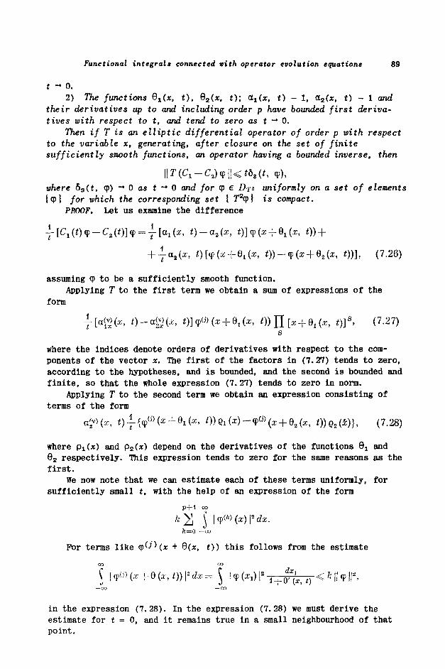
Functional integrals connected with operator evolution equations 89

t - 0.

2) The functions θ^χ, t), Qs(x, t); а

г(х, t) - 1. 0L

2(x, t) - 1 and

their derivatives up to and including order ρ have bounded first deriva-tives with respect to t, and tend to zero as t — 0.

Then if Τ is an elliptic differential operator of order ρ with respect

to the variable x, generating, after closure on the set of finite

sufficiently smooth functions, an operator having a bounded inverse, then

— C.) φ || < ίβ, (ί, φ),where 6 3 (t , φ) ~* 0 as t ~* 0 and for φ 6 D-rz uniformly on a set of elements{cpi for which the corresponding set { 7^φ I is compact.

PROOF. Let us examine the difference

(7.26)

assuming φ to be a sufficiently smooth function.

Applying Τ to the first term we obtain a sum of expressions of the

form

у [<>(*, t)-a%>(z, m ^ i x + Q^z, t))J[[x + e

i{z,

t)f, (7.27)

s

where the indices denote orders of derivatives with respect to the com-ponents of the vector x. The first of the factors in (7.27) tends to zero,according to the hypotheses, and is bounded, and the second is bounded andfinite, so that the whole expression (7.27) tends to zero in norm.

Applying Τ to the second term we obtain an expression consisting ofterms of the form

<v)(x, Q-l-iqPiz + e^z, t))Qi(x)-^(

x + e

a(z, f))Q«(*)b (7.28)

where Pi(x) and P2(*) depend on the derivatives of the functions Bj and

θ2 respectively. This expression tends to zero for the same reasons as the

first.We now note that we can estimate each of these terms uniformly, for

sufficiently small t, with the help of an expression of the form

P+l oo

/с 2 \ \<fw(x)\*dz.

fe=0 —со

For terms like φθ')(* + 9(*, t)) this follows from the estimate

CO CO

\ \<pa(z + e(z,t))\*dz=: J Ιφ(*ι)1

in the expression (7.28). In the expression (7.28) we must derive theestimate for t = 0, and it remains true in a small neighbourhood of thatpoint.

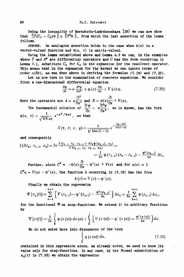
90 Yu.L. Daletskii

Using the inequality of Bernstein-Ladyzhenskaya [20] we can now show

that ||r<d. - С2)Ф \\κ \\Τ*φ ||, from which the last assertion of the lemma

follows.

REMARK. An analogous assertion holds in the case when φ(χ) is avector-valued function

1 and Λ(χ, t) is matrix-valued.

Using the lemma established above and Lemma 4.5 we can, in the exampleswhere Τ and A" are differential operators and С has the form occurring inLemma 7.1, substitute C

x for C

2 in the expansion for the resolvent operator.

This means that in the expansion for the kernel we can ignore terms of

order ο(Δί), as was done above in deriving the formulae (7.18) and (7.23).Let us now turn to the examination of concrete equations. We consider

first a one-dimensional differential equation

& = «-3- + ф(*>-2-+Г(*>*. (7-29)

92 Э

Here the operators are A = o j l and Β = φ(χ)?τ~ + V(x).OX — —ο ΟΧ

σ ψ σ ψThe fundamental solution of — — = α—-5-, as is known, has the form

ot οχy(

Xt t) = e " *

2 / 4 a t, so that

/ 4 К t/ 4 К at

S (τ, t; x, y)=

and consequently

\_in .i), x

h) __

= i Ψ (fc-i) (% - 4-1) -

Further, since C* = - Ф * * ) ^ - Ч>'(*) + ν(χ) and for u(x)

C*u = V{x) - φ'(χ), the function h occurring in (7.18) has the form

Finally we obtain the expression

n+l n+1

fe=l

for the functional Ψ on step-functions. We extend it to arbitrary functions

by

5 | $b 0

We do not enter here into discussion of the termr

J φ (χ (и)) du, (7.30)0

contained in this expression since, as already noted, we need to know its

value only for step-functions. In any case, by the formal substitution of

Xq(t) in (7.30) we obtain the expression

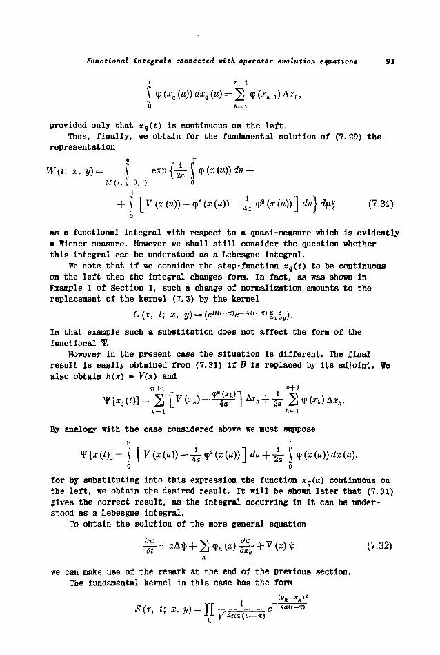
Functional integral» connected with operator evolution equation» 91

< n-j-i

J φ К (м)) «Цг (в) = 2 Φ fo-i)

Δ^>

Ό ft=i

provided only that #g(f) is continuous on the left.

Thus, finally, we obtain for the fundamental solution of (7.29) the

representation

* +

W(t;x,y)= J exp {— J φ {χ (и)Μ (χ, у; 0, ί) О

+

+ J [ F (χ (в)) - φ' (х (и)) - ± φ2 (χ (и)) ] duj άμν (7.31)

о

as a functional integral with respect to a quasi-measure which is evidently

a Wiener measure. However we shall still consider the question whether

this integral can be understood as a Lebesgue integral.

We note that if we consider the step-function Xq(t) to be continuous

on the left then the integral changes form. In fact, as was shown in

Example 1 of Section 1, such a change of normalization amounts to the

replacement of the kernel (7.3) by the kernel

In that example such a substitution does not affect the form of the

functional Ψ.

However in the present case the situation is different. The final

result is easily obtained from (7.31) if β is replaced by its adjoint. We

also obtain h(x) = V(x) and

«+i _ _.,.. ,„ , n+i

Ψ iX (t)] = ^

By analogy with the case considered above we must suppose

+ ι

Ψ [χ (t)] =l[V{x (в)) - ± φ2 (χ (и)) ] da + ± J φ (χ (и)) dx (в),

5 о

for by substituting into this expression the function xq(u) continuous on

the left, we obtain the desired result. It will be shown later that (7.31)

gives the correct result, as the integral occurring in it can be under-

stood as a Lebesgue integral.

To obtain the solution of the more general equation

ψ (7.32)

.ν

we can make use of the remark at the end of the previous section.

The fundamental kernel in this case has the form

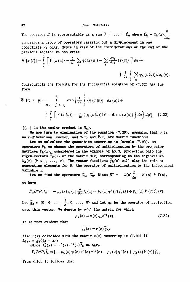
92 Yu.L. Daletskii

The operator В is representable as a sum 3i + ... + β* where β^ φ ( W

generates a group of operators carrying out a displacement in one

coordinate xk only. Hence in view of the considerations at the end of the

previous section we can write

0 ft

Consequently the formula for the fundamental solution of (7.32) has the

form

* t

W(t; x, y)= ξ expj-^-J (φ(ζ(Β)), dx(u)) +Μ (*

ν ~j; o, t) о

t

4-j [7(χ(α))-^-((φ(χ(Μ))))2_(1ίνφ(ζ(

Μ))]ώ}ώμν. (7.33)

о

({, ) is the scalar product in Rm).

We now turn to examination of the equation (7.29), assuming that ψ isan г-dimensional vector, and φ(χ) and V(x) are matrix functions.

Let us calculate the quantities occurring in formula (7.23). Asoperators P* we choose the operators of multiplication by the projectormatrices Pfc(x) _ considered in the example of §5.3, projecting onto theeigen-vectors fk(x) of the matrix cp(x) corresponding to the eigenvalues

Xfe(x) (k = 1 r). The vector functions /*(*) will play the role of

generating elements for B, the operator of multiplication by the independentvariable χ. ~

Let us find the operators C'u C'

2. Since Β* = - φ ( χ ) — - φ'(χ) + V(x),

ox

we have

ox

Let gk - (0, 0 —, 0, .... 0) and let qk be the operator of projection

onto this vector. We denote by v(x) the matrix for which

Ph \х) —

v \

x) 4k

v \

ΧΙ· \' ·°^)

It is then evident that

Also v(x) coincides with the matrix v(x) occurring in (7.23) if

fexo 1

Since fk(x) = v'(x)v~1(x)fk we have

PhB*P

hfh = [-p

h{x)<¥ {x) V (x) v'

1 {x) -

Pk (χ) ψ' (x) +

Ph (x) V (x)] f

k,

from which it follows that

ч ч(*"чх) ,ώ [Г - «Jу Г"*) Л [^ + ч* V ί1""*

-у - {Χ'4χ ~4χ) {Χ~4χ) ώ έ f+ bv (ι'4χ) г<ь £ -у - {Χ'4χ ~4χ) {Χ~4χ) ώ έ f"= [(ί) δ

nuoj aqq. звц ^ xeuoT^ounj эщ ээво ^irasajd щ% щ 'snqi

ЭАВЦ эм '(^ε'Λ) - q 'ΧΤ-ΙΪΒΠΙ хвиоЗвтр в sf II ifq ίχ || = V

'(χ) г_п (χ) γ (χ) α = (ж) ώ

звц

jo λ Х|Д вш эц^ SB sjBaddB эртз ривц-^чЭтд ац^ uo Х|д^вш•(χ) ώ (χ) χ_η (χ) ,α + (χ) ,ώ - (г) Л = ί3

) т .я (г) ,α (χ) ώ + (χ) ώ (χ) T_f2 (χ) μ — (χ) ,ώ =

== {(χ) т,д (χ) ,β (χ) V (г) ώ + (χ) 4 (χ) Τ.β (χ) ,α (χ) V (χ) ώ -

(χ) ώ (χ) 4 {χ) χ_α (χ) ,α (χ) V + (χ) ώ (χ) 4 (χ) т_я (χ) ,α - ,[(χ) ώ (χ) V]} £

= {(χ) ?</ (χ) V (χ) ώ - (χ) ώ (χ) 4 (χ) у - Д(х) Ч (χ) * (χ) 4]} £ =

з{двшэл эм J T pauuojsuBJ^ц

aq UBO uoissajtdxa ^SBI aqx -Q = (χ)4ά(χ)τ_α(χ)ia(x)4d ^ '(frS'L) jCq 'aoujs

'(x) V (x) ,ώ (χ) 4 £ - (χ) t. f l (χ) / β (χ) ώ + (χ) Л = (χ) 4 (χ) ,ώ (χ) ч £ -ц уфС

- (χ) 4 (χ) ,_я (χ) ,α (χ) V (χ) ώ £ - (χ) V (χ) τ_α (χ) / β (χ) V (χ) ώ ζ + (χ) Л =

•JCXXBUTJ рив

(x) V (x) Л (χ) frf + (χ) 4 (χ) t.o (x) ,β (χ) ώ (χ) сйГ -

= (*) V (χ) л (х) fd + (x) у (χ) ώ (χ) cc/ = VffCс/ЭЛВЦ ЭМ OS

'(χ) τ_β (χ) /β(χ) V - ( χ ) 4 (χ) Τ.β (χ) ,β = (χ) У

SMOXXOJ aaaq^ (^g'L) moaj asnBoaq '

•(x) 4 (χ) τ,β (χ) ,β (χ) ώ (χ) 4 —

- (χ) ч (χ) л (χ) ч + (χ) ад (χ) ,ώ (χ) ад - = ν Cff) (,,vV

£6 suotjoni» uoijnjons Jo}Djsdo 4}in рэ}ээииоэ

94 Yu.L. Daletskii

and so the fundamental matrix of the system (7.29) is representable as afunctional integral

W(t;x,y)= ^ eiTpji j φ (a, (u)) &c (u) +Μ (ж, у; о, о χ

t

+ \[V(x (и)) - φ' (χ (и)) - ф 2 ( | а

( ц ) ) + 2ι>' (х) о"! (х) φ (а; (и)) ] duj άμ».χ

We can pass in th i s way to the system

| £ = α Δ ψ + 2 φ α * ) ^ - + Γ(*)Μ> (7.35)ft

with matrix functions фд(эс), ^(*) Just as in the case of a single equation.We thus have

T H E O R E M 7.3. The fundamental matrix of the system (7.35), where

<Pfe(*). V(x) are sufficiently smooth, bounded matrix functions, and the

(Pfe(x) are symmetric, is representable as a functional integral with res-

pect to the Wiener measure:

ξ { ^ *<*g

( l t ) ) , dx(u))

M(x, y;

I [4

^ ] .о

(7.36)where i>fe(x) is a matrix reducing cpfc(x) to diagonal form.

REMARK. We could also examine the case when the coefficients dependon t. The final formula (7.36) does not change.

5. The relation of functional integrals generated by diffusionequations with Lebesgue integrals with respect to the Wiener measure.

In the examples examined in the previous section the quasi-measurewas non-negative and arose in a way not unlike the Wiener measure consider-ed on quasi-intervals. The question therefore arises naturally: arefunctional integrals Lebesgue integrals with respect to the Wiener measure?

A similar question was considered in §2 where it was stated that, forfunctionals depending only on the values of the function at a finitenumber of points, the answer to this question is in the affirmative. Inparticular for any functional Φ[χ(ί)] the equation (2.3) holds:

$ \ , (7.37)Μ Μ

In order to pass to functionals Φ which depend on all the values ofx(t) we must, in (7.37), be able to go to the limit as d(q) - 0.

For this the following conditions must be satisfied:1) Φ[*(ί)] must be continuous for some topology in which

x(t) = lim xq(.t), so that Φ [x(t) ] = lim Φ ix

q(t) ] for each function x(t)

q я

in a set of full Wiener measure.

2) A condition allowing us to pass to the limit under the integral

Functional integrals connected with operator evolution equations 95

sign in (7.23) must be satisfied.Consider the first condition. Since the Wiener measure is concentrated

on the continuous functions, and for such functions the sequence xq(t)

converges uniformly to x(t) as d(q) — 0, the first condition is satisfiedif the functional is continuous in the uniform topology.

In particular, functionals of the formt

exp С V [χ {и)] du, (7.38)ό

where V(x) is continuous, have this property.

However in (7.33) and (7.36) we meet functionals of the formt

5 f(x(u))dx(u), (7.39)о

which do not have this continuity. Incidentally, since x(u) is not, as arule, of bounded variation it is still necessary to say in what sense theintegral (7.39) is to be understood.

Such integrals are considered in the theory of random processes, wherethey are called stochastic integrals. It turns out that they exist in thefollowing sense [45]:

t n+l

\f{x (и)) dx (u) = lim 2 / (Ч-ι) Axk,

о « h=i

where the convergence is understood as mean-square convergence withrespect to the Wiener measure, i.e.

t n+i

$[$/(* («)) dx (и) - 2 f (x^) Axk 1 άμ _> 0.

Μ ' 0 h=i

From a sequence convergent in mean we can always extract a subsequenceconvergent almost everywhere.

In this way, if Ф(дс) has the form

Φ (χ (и)) = βψ <* (")), (7.40)

where Ψ(*) contains integrals of the type (7.39), and ordinary integrals,

then there always exists a sequence of subdivisions gn for which, on a

certain set of functions x(t) having full measure,

*V[x(u) ] = lim Ψ[*,η(ΐί) ] , and hence

η — a>

Φ[ΐ(«)]=1ύηΦ[ϊ («)]. (7.41)п-юэ

We now turn to discussion of the second condition. The boundednessof the functional Ф(х) is the simplest condition allowing us to go to thelimit. Under this condition the sequence of functionals <t>

q(x) will be

uniformly bounded, and if it also converges to Ф(*) then we can pass tothe limit in (7.37).

We obtain the following result, a particular case of a more generaltheorem proved in [з].

THEOREM 7.4. If Φ ix(u) ] is a bounded functional, and

96 Yu.L. Daletskii

ПшФ[хд(и)]=Ф[х(и)}

Q

for almost all v(x), in the sense of the Wiener measure, then*J Φ [x (it)] άμ = J Φ [x {u)} άμ.

Μ Μ

C O R O L L A R Y . The integral in (7.6'), which gives, in particular,for A = Δ, the solution of the differential equation

coincides with the Lebesgue integral. We obtain in this way a theorem ofM. Kac [2], at least for the case of a bounded smooth function V(x, t).

The result remains correct if instead of the Laplacian we take anyother self-adjoint, non-positive elliptic operator of the second order. Wecan also consider the problem not in the whole space but in a domain if wetake the operators with certain boundary conditions.

The quantityt

\ exp 1 \ V (x (u)) dui άμΜ О

ί

is none other than the mean value of the functional exp \ V(x(u))du

Όin the random process with probability distribution given by the Wiener

measure, i.e. in the so-called Brownian movement. It follows from Theorem

7.4 that

t

^ exp [ V (x (u)) du } άμ = lim \ exp [ У(хк_г) At

k ] άμ*. (7.42)

м г " т

The integral on the right-hand side of this equation is the mean in a cer-

tain random process, but with a discrete time, i.e. in a certain Markov

chain.

Considering instead of V the functional zV we obtain for each of these

processes the characteristic function of the random variablet

\ V (x (u)) du. In this way (7.42) shows that the characteristic function

ό t

of the functional \ V(x(u))du in the Brownian movement is the limit of

bthe characteristic functions of the functional considered on certainprocesses with discrete time. In other words the equation represents acertain limit theorem in the theory of random processes.

As the functional (7.40) examined above contains stochastic integralsit does not satisfy the conditions of Theorem 7.4, for, although (7.41) issatisfied for a certain sequence of subdivisions, the functional is notbounded.

Functional integrals connected with operator evolution equations 97

The problem, it is true, is simplified in that the existence of the

functional integral in the case connected with the differential equation

(7.32) is known a priori, i .e. it is known that the sequence of integrals

e^V"» άμ (7.43)

converges. If we choose some other differential equation of the form (7.32):

for which the corresponding functional 1Ί has the form

Ψχ = 2Ψ,

we can show the convergence and hence the boundedness of the sequence of

integrals

С e2W[*

a(u)]

d~

Μ

In th i s way the sequence of functionals Φ(χ) = e ^ has the properties:1) Φ [χ (и)] — Φ[x(u) ] almost everywhere with respect to the

inWiener measure;

2) С Φ 2 [xqn (и)] άμ<0 for all п.м

In accordance with a well-known theorem of the theory of functions i tfollows from these conditions that

lim \ Φ K n («)] άμ=[φ[χ (и)] άμ.9 м Μ

In this way we proveTHEOREM 7.5. The fundamental solution of the differential equation

(7.32) with sufficiently smooth coefficients is representable as an integral

W(f,x,y)= ξΜ(χ, ν, Ο,ί)

with respect to the Wiener measure, where

~ J (φ (χ (α)), dx(u)) +о

ί

+ 5 [v(x(u))-±-{(<f(x(u))))*-div<p]du}. (7.44)

This integral is also a functional integral in our sense, i.e. is the limit

of a sequence of finite-sum integrals

ΦΙ*β(Β)]<*μ&. (7.45)

The formula (7.44) means that the measure generated by the fundamental

98 Yu.L. Daletskii

solutions of (7.32) is absolutely continuous with respect to the Wienermeasure, and the expression under the integral sign is the density of thismeasure with respect to the Wiener measure.

A result of this type was first obtained for the one-dimensionaldiffusion equation in [23]. The formula (7.44) was derived by heuristicarguments in [7]. This formula also follows from the results obtained in[24].

The formula (7.45) admits of a probabilistic interpretation as acertain limit theorem analogous to that noted above, after Theorem 7.4.

The results considered in the present section can be extended to thecase of a system of equations instead of a single equation. Theorem 7.4goes over completely, and Theorem 7.5 under the further assumption thatthe matrices <p& are diagonal, and the matrix V satisfies the conditions

vjh>o и Φ щ.

Under these conditions the matrix

w — К*

е Sjn Suy)

has non-negative elements. In this case we can give a probabilistic inter-pretation to the system of equations (7.35), as has already been remarkedin §2.

§8. The representation of generalized kernels as weakfunctional integrals

I. Functional integrals corresponding to generalized solutions.

Let us examine an equation of the form

- ^ = ψ+£ψ, (8.1)

where A is a self-adjoint operator. For simplicity we shall consider onlyequations with constant coefficients, although certain results remaintrue also for equations with variable coefficients, and we shall indicatethis in the appropriate places.

We shall suppose that the conditions of Theorem 4.4 are satisfied, sothat we have the representation

e(tA+B) «ξ _ ;

ч k=i

for the resolvent.The fundamental solutions and kernels, unlike the case considered in

the previous section, are here generalized elements, and the expansion

n+l

W(t; x, y) = (β<ίΑ+

Β)

ίξ

χ,ξ

ν) = lim \ Π (e

lAU'

he

BA'

hix. , ξχ ) da (xj ...da(x

n)

" S3? h=i

(8.2)

must be understood as convergent in the weak sense, as described in §6.2.

Functional integrals connected with operator evolution equations 99

Prom a formal point of view the calculations in the present case donot differ from those of §§7.1 and .2.

Let us suppose that В operates on generalized eigen-elements S,jx of

the spectral set Ε(Δ), which satisfies the condition ( Ш . 1 ) , by the

formula

Ь}х — ZJ ujk У·*') Чкх·

Also, as before,

G { Τ f ' Τ 7/^ V ί Τ / τΛ S ίX t' Ύ ll\V l1 "·! χ ) У) — Υ V^i *· l j " ^ 1 | ι ) ·*-» У}ι

where the matrix γ i s of the form γ = exp tb(x).In t h i s way i t follows from (8.2) t h a t

W (t; x, y) = lim ^ у (x0, Δ^) S (0, i x; x0, xx) у (xx, Δί2) . . .

. . . γ (χη, Δί η + 1 ) S ( ί η , ί; a;n,y) da (Ж1) ...da (xn), (8.3)

and by the definition given in §6.2 we obtain the following result:T H E O R E M 8.1. The fundamental matrix of the equation (8.1), (which

satisfies the conditions of Theorem 4.4), corresponding to the system£jχ 0 = 1 · ····

m>

x e ^ Г ) of generalized eigen-elements of the spectral

set Ε(Δ), (which satisfies the condition (III.l)), is, on the assumptionthat В commutes with the set Ε(Δ), representable as a weak functionalintegral

* t

W(t\ x, y) = (T) \ exp j \ b {x(u)) du\ άμ8 [χ (и)]. (8.4)

M(x,'y;0,t) 0

The analogous result is true when the operators depend on t.Let us now suppose, in addition, that A is non-positive. As follows

from Lemma 6.3, the fundamental solutions of

-^- = (i — ε) Aty + Cib (8.5)'ot

tend, as ε -· 0, to the fundamental solutions of (8.1), in the sense of

strong convergence of generalized elements.

The fundamental kernel of (8.5) can be represented in the form

M(x, y; 0, i)

where the functional integral is understood in the ordinary sense, as the

equation (8.4) satisfies the conditions of Theorem 4.3 for ε > 0.

Since we have the relation W(t; x, y) = lim WP(t; x, y) in the sense

ε - ο ε

of weak convergence of generalized functions of x, we obtain the followingresult :

THEOREM 8.2. If, under the conditions of Theorem 8.1, the operatorA is semi-bounded, then the generalized fundamental kernel W(f, x, y) of

100 Yu.L. Daletskii

equation (8.1) is representable as a limiting functional integral

* * t

W{t; x, y) = Τ \ exp [ \b (x(u)) duΊ άμ8 [χ{и)]. (8.6)Μ 0

REMARK. If we take into account the remarks after Theorem 4.4 andLemma 6.3 then we can also examine the case when В is unbounded andgenerates a hyperbolic group. We do not set out the results, as the formalcalculations do not differ from those of §7. 3 and the nature of the con-vergence is the same as in Theorems 8.1 and 8.2.

The sign (T) in the formulae (8.4) and (8.6) can, as usual, be removedif either the transition function S(T, t; x, y) or the functionalί

\ b (x(u))dutskes scalar values.о

EXAMPLE. Let us examine the differential equation

where L is an elliptic operator. In the examples of §4.5 it was shown thatunder given conditions of smoothness on the coefficients in the equation,Theorem 4.4 applies. Consequently we can also apply Theorem 8.1 and, if Lis semi-bounded, Theorem 8. 2.

In this way the fundamental kernel of the equation is representable asa weak functional integral

t

* fv(x(u), u) duW(t;x,y) = ξ

eo άμ

Β[χ(α)] (8.7)

M(x, y. 0, ί)

with respect to the generalized quasi-measure μ$ generated by the

fundamental kernel of the equation "5^= ϋ ψ · It follows from (8.7) that

if ψ(χ, t) is the solution of the equation corresponding to an initialvalue which is a basic function, then

CO

Ψ (У, 0 = 5 Ψ (*. 0) W(t; χ, у) da (χ) =—oo

n+1

ψ (x0, 0) eh=l Д S ( f k . l t i f c, я , , . ! , ж) Лг (а:0) . . . d a (ж„).ft

(8.8)

5

Rq

The integral in this formula is to be understood as in §R.2. it must becalculated in the order which corresponds to the order of the differentials.

On the other hand if L is semi-bounded the integral can be understoodas a limiting integral, i.e.

* t

ψ (у, t) = lim [ ψ (x, 0) \ exp Я V (x (и)) du} άμ^,ε"*° Βχ M(0,t;x,y) 0

Functional integrals connected vith operator evolution equations 101

where μ^ is the quasi-measure generated by the fundamental kernel of theequation

•£ = («-e)L*.

and for ε > 0 the functional integral can be understood in the ordinarysense.

In particular, for ί,ψ = α Δ ψ we obtain a foundation for the integralsrelated to Schredinger's equation introduced by Feynman. The transitionfunction for these integrals is given by the formula

S (τ, t; x,y) = -7

(1/-*)'

ί (ί — τ)

and so is a kernel which is smooth but not square-summable. The quasi-measure in this example is an ordinary function, and so the finite sumintegrals

n+l n+l

ψ (x0, 0) exp 1 2 V (x

k_j) Ai

fc j- Д S (х

к.1г x

h; At

h) da (x

0) ...da (x

n)

yx y

n fe=i fe=i

between finite limits of integration, can be understood in the usual sense,however, when the limits become infinite, the integrals must be understoodas generalized functions which have regularizations in the sense

n+i

{lim V( X

• • · da(xn).

n+l

ν TT я it t · τX Д o

E{i

h_

v i

h, x

ft.x, ,

ft=l

We observe that all these equations can be considered not only in thewhole space, but also in a part of the space, with given boundary condi-tions. This was discussed in more detail in §4.5.

Further, instead of one equation we can examine systems. For example,for a system of the form

ft=l

where

cr, =01

10 , σ 2 _

0

i

— i

0 ' °3~10

0j

are the so-called Pauli matrices examined in [46], the fundamental matrixhas the form

м

exp | \ [a^! (и) + σ2χ2 (и) + a

sx3(и)] daY άμ

8,

о

where μ5 is the same Feynman quasi-measure as in the case of the Schredinger

equation, and the matrix

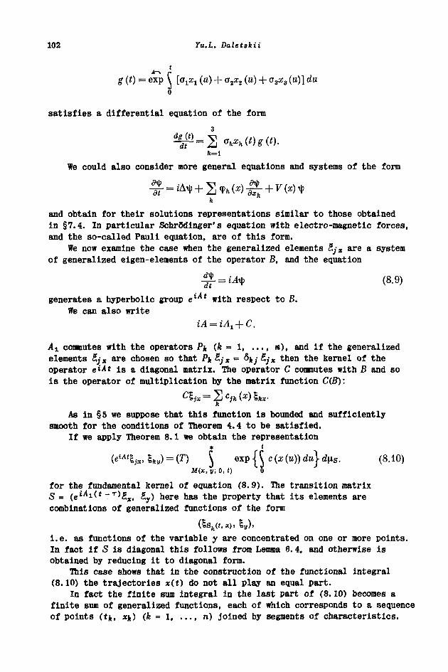
102 Ya.L. Daletskii

t

g (t) = exp [ σ ^ (и) + агх

г (и) + σ

3χ

3 (и)] du

о

satisfies a differential equation of the form

3

We could also consider more general equations and systems of the form

k

and obtain for their solutions representations similar to those obtained

in §7.4. In particular Schrodinger's equation with electro-magnetic forces,

and the so-called Paul! equation, are of this form.

We now examine the case when the generalized elements £jx are a system

of generalized eigen-elements of the operator B. and the equation

^ = iAy (8.9)

generates a hyperbolic group elAt with respect to β.

We can also write

Αχ commutes with the operators Pfc (k = 1 in), and if the generalized

elements £jx are chosen so that Pk £/* = &kj £jx then the kernel of the

operator eiA* is a diagonal matrix. The operator С commutes with В and so

is the operator of multiplication by the matrix function C(B):

h

As in §5 we suppose that this function is bounded and sufficiently

smooth for the conditions of Theorem 4.4 to be satisfied.

If we apply Theorem 8.1 we obtain the representation

\ { $ } (8.10)M(.x,y;0,t)

for the fundamental kernel of equation (8.9). The transition matrixS = (elAi(·* ~r^tx, 5y) here has the property that i ts elements arecombinations of generalized functions of the form

(isft(<, ж). E

y) ,

i.e. as functions of the variable у are concentrated on one or more points.

In fact if S is diagonal this follows from Lemma 6. 4, and otherwise is

obtained by reducing it to diagonal form.

This case shows that in the construction of the functional integral

(8.10) the trajectories x(t) do not all play an equal part.

In fact the finite sum integral in the last part of (8.10) becomes a

finite sum of generalized functions, each of which corresponds to a sequence

of points (tfc, xk) (fe = 1, ..., n) joined by segments of characteristics.

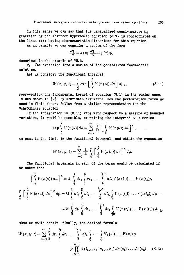
Functional integrals connected with operator evolution equations 103

In this sense we can say that the generalized auasi-measure \i$generated by the abstract hyperbolic equation (8.9) is concentrated onthe lines x(t) having characteristic directions for this equation.

As an example we can consider a system of the form

described in the example of §5.3.2. The expansion into a series of the generalized fundamental

solution.Let us consider the functional integral

* i

W (x, y, t) = ξ exp [ $ F (x (u)) du ] άμ8, (8.11)

Μ О

representing the fundamental kernel of equation (8.1) in the scalar case.It was shown in [7], by heuristic arguments, how the perturbation formulaeused in field theory follow from a similar representation for theSchr6dinger equation.

If the integration in (8.11) were with respect to a measure of boundedvariation, it would be possible, by writing the integrand as a series

i 00 t

exp J V (x (в)) du = 2 χρ [ [ V (x (u)) du] k ,

0 fc=0 ' 0

to pass to the limit in the functional integral, and obtain the expansion

00 t

k=0 4 0

The functional integrals in each of the terms could be calculated ifwe noted that

[ ]v(x(u)) du] = k\ J dt, J dt, . .. ξ dtkVixita) ... V(x(th)),

ο ό Ό ο

МО О О О Μ

589

Thus we could obtain, finally, the desired formula

« t h (k-i

\ 1С/' / J^J · v» | . w IJ • f · . Д 1

fc=0 0 0 0 S3

n+1

χ Д S(th_v tk; xk_v xk) daixj . . . da(xn). (8.12)

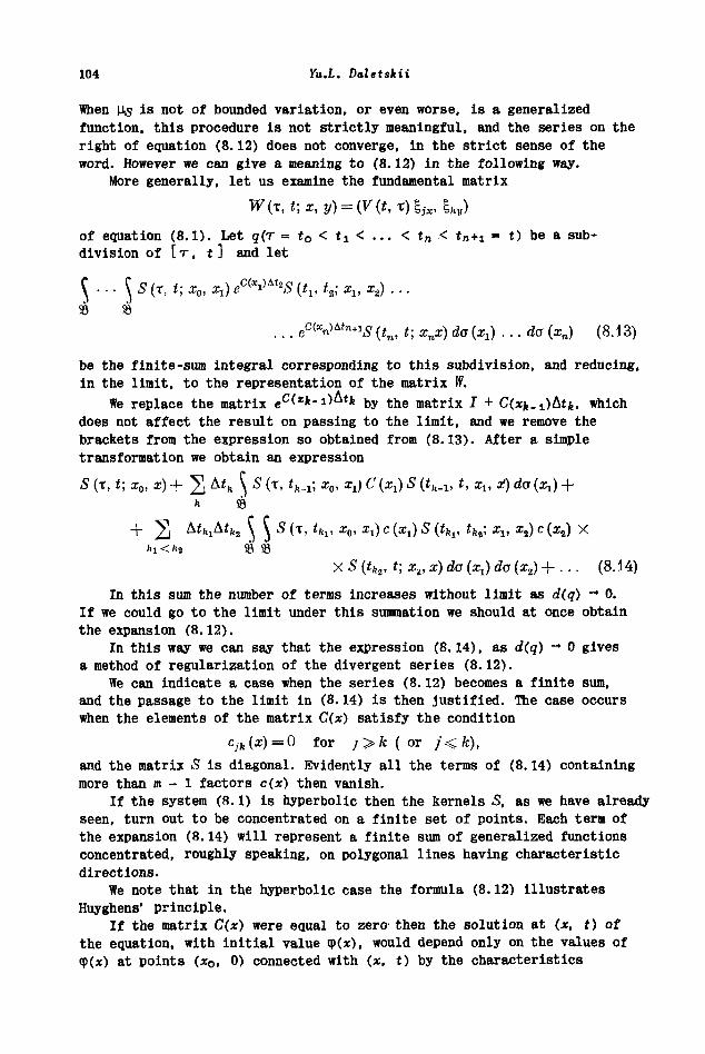
104 Yu.L. Daletskii

When \is is not of bounded variation, or even worse, is a generalizedfunction, this procedure is not strictly meaningful, and the series on theright of equation (8.12) does not converge, in the strict sense of theword. However we can give a meaning to (8.12) in the following way.

More generally, let us examine the fundamental matrix

of equation (8.1). Let q(r = t0 < tj. < ... < t

n < tn+i = t) be a sub-

division of [ τ , t ] and let

^ S (t, t; x0, x

x) e

c{xJ^S (t

v t

a; x,, z

2

93 58

be the finite-sum integral corresponding to this subdivision, and reducing,in the limit, to the representation of the matrix W.

We replace the matrix e

c(

xk-i)^k by the matrix I + C(xjfe.

1)Atfe. which

does not affect the result on passing to the limit, and we remove thebrackets from the expression so obtained from (8.13). After a simpletransformation we obtain an expression

S (t, t; x0, x) + 2 Ai

h ^ S (τ, t

k_

i; x

0,

Xl) С (x

x) S (i

h.x, t,

Xl, af) da (х

г) +

\ 5bi<k

2 SB 93

X 5 (th2, t; x.., x) da {xj da (x

2) + . .. (8.14)

In this sum the number of terms increases without limit as d(q) — 0.If we could go to the limit under this summation we should at once obtainthe expansion (8.12).

In this way we can say that the expression (8.14), as d(q) - 0 givesa method of regularization of the divergent series (8.12).

We can indicate a case when the series (8.12) becomes a finite sum,and the passage to the limit in (8.14) is then justified. The case occurswhen the elements of the matrix C(x) satisfy the condition

cjh i

x) — 0

f o r / > Λ ( ОГ / < к),

and the matrix S is diagonal. Evidently all the terms of (8.14) containingmore than m - 1 factors c(x) then vanish.

If the system (8.1) is hyperbolic then the kernels S, as we have alreadyseen, turn out to be concentrated on a finite set of points. Each term ofthe expansion (8.14) will represent a finite sum of generalized functionsconcentrated, roughly speaking, on polygonal lines having characteristicdirections.

We note that in the hyperbolic case the formula (8.12) illustratesHuyghens* principle.

If the matrix C(x) were equal to zero then the solution at (x, t) ofthe equation, with initial value cp(x), would depend only on the values ofφ(χ) at points (x

0, 0) connected with (x, t) by the characteristics

Functional integrals connected vith operator evolution equations 105

Sk(t, x).

If we consider that each characteristic describes the distribution, in

the phase space, of a wave of a certain type, then in this simplest case

the waves do not interact with each other.

If C(x) 4 0 then such an interaction does take place, and is describedby the further terms of the series (8.12).

Received by the editors, 8th March, 1962.

Bibliography

[l] R.P. Feynman, фасе-time approach to non-relativistic quantum mechanics,Rev. Mod. Phys. 20, 2 (1948), 367-387. (Russ. Transl., IL, 1955).

[2J M. Kac, On distributions of certain Wiener functionals, Trans. Amer. Math.Soc. 65. 1 (1949), 1-13.

[3] S. V. Fomin, On the inclusion of the Wiener integral in a general theory ofthe Lebesgue integral, Nauchn. Dokl. Vyssh. Shk., Fyz.-Matem. Nauki, 2 (1958).

[4] L.N. Slobodetskii, On the fundamental solution of the Cauchy problem for aparabolic system, Matem. Sb. 46 (88): 2 (1958).

L5J W. Feller, Diffusion processes in one dimension, Trans. Amer. Math. Soc.77(1954), 1-31. (Russ. Transl., Matematika 2 (1958), 119-146).

[б] Ε.Β. Dynkin, Infinitesimal operators in Markov processes, Teoriya Veroyatn.i ее Prim. 1 (1956), 38-60.

Ы I.M. Gelfand and A.M. Yaglom, Integration in functional spaces, UMN 11, Pt.1 (67) (1956). 77-114.

[δ] Ε. Hille,- Functional analysis and semigroups, New York, 1948. (Russ. Transl.Funktsional' nyi analiz i polugruppy, Moscow, IL, 1957.)

[9] T. Kato, Integration of the equation of evolution in a Banach space, Journ.Math. Soc. Japan, 5 (1953). (Russ. Transl., Matematika, 2:4 (1958)).

[io] M.A. Krasnosel'skii, S.G. Krein and P.E. Sobolevskii, On differentialequations with unbounded operators in Hilbert space, Dokl. Akad. Nauk., 112,No. 6 (1957).

[ll] S.G. Krein and P.E. Sobolevskii, Differential equations with an abstractelliptic operator in a Hilbert space, Dokl. Akad. Nauk., 118, No. 2 (1958),233-236.

[12] P.E. Sobolevskii, On equations of parabolic type in a Banach space, TrudyMosk. Matem. Obshch. (10) (1961), 297-350.

tl3] P. D. Lax, On Cauchy's problem for hyperbolic equations and the differenti-ability of solutions of elliptic equations, Comm. Pure Appl. Math., 8 (1955).(Russ. Transl., Matematika, 1: 1 (1957)).

[14] G. I. Kats, Generalized elements of a Hilbert space, Ukr. Matem. Zhurn.,12, 1 (1960), 13-24.

[15] I.M. Gelfand and G.%. Shilov, Certain questions in the theory of differen-tial equations, Moscow, FMzmatgiz, 1958.I.M. Gelfand and A.G. Kostyuchenko, On expansions in eigen-functions fordifferential and other operators, Dokl. Akad. Nauk., 103, No. 3 (1955),349-352.

[17] Yu.M. Berezanskii, On expansions in eigen-functions of general self-adjointdifferential operators, Dokl. Akad. Nauk., 108, No. 3 (1956), 379-382.

[ΐδ] G. I. Kats, On expansions in eigen-functions of self-adjoint operators, Dokl.Akad. Nauk., 119, No. 1 (1958), 19-22.

[19] 0. A. Ladyzhenskaya, A simple proof of the solvability of fundamentalboundary-value problems and problems concerning the eigen-values of linearel l iptic equations, Vestn. Leningrad Univ. 11 (1955), 23-30.

106 Yu.L. Daletskii

[20] 0. A. Ladyzhenskaya, On integral estimates, convergence of approximationmethods, and solutions of linear elliptic equations, Vestn. Leningrad Univ.7 (1958), 60-69.

[21] 0.V. Guseva, On boundary-value problems for strongly elliptic systems, Dokl.Akad. Nauk., 102, No. 6 (1955), 1069-1072.

[22] M. Schechter, Integral inequalities for partial differential operators andfunctions satisfying general boundary conditions, Comm. Pure Appl. Math.,12 (1959).

[23] Yu.V. Prokhorov, The convergence of random processes and limit theorems ofthe theory of probability, Teoriya Veroyatn. i ее Prim. 1 (1956), 177-238.

[24] A.V. Skorokhod, On the differentiability of measures corresponding torandom processes, II, Teoriya Veroyatn. i ее Prim. 5, No. 1 (1960).

[25] Yu.L. Daletskii, On the representability of solutions of operator equationsas functional integrals, Dokl. Akad. Nauk, 134, No. 5 (1960) 1013-1016.(Translation: Soviet Math. Doklady 1 (1960) 1163-6).

[2б] Yu.L. Daletskii, Fundamental solutions of operator equations and functionalintegrals, Isv. Vyssh. Zav., Matem. 3 (22) (1961), 27-48.

[27] Yu.L. Daletskii, Functional integrals connected with certain differentialequations and systems, Dokl. Akad. Nauk. 137, No. 2 (1961), 268-271.(Translation: Soviet Math. Doklady 2 (1961) 259-263).

[2δ] R.H. Cameron, A family of integrals serving to connect the Wiener andFeynman integrals, Journ. of Math, and Phys. 39, No. 2 (1960).

[29] Yu.L. Daletskii, Functional integrals and characteristics connected with agroup of operators, Dokl. Akad. Nauk, 141, No. 6 (1961) 1290-1293.(Translation: Soviet Math. Doklady 2 (1961) 1634-1637).

[30] A.N. Kolmogorov, On analytical methods in the theory of probability, Uspehi.Mat. Nauk. V (1938), 5-41.

[31] A.N. Kolmogorov, Basic concepts of the theory of probability, (Osnovyeponyatiya teorii veroyatnostei) Moscow Leningrad, ONTI, 1936.

[32] M. Kac, On some connections between probability theory and integralequations, Proc. 2nd Berkeley Sympos. Math. Stat. and Probab., Berkeley(1951), 189-215 (Russ. Transl. Matematika 1: 2 (1957), 95-124).

[33] F.R. Gantmakher, Teoriya Matrits, Moscow, Gostekhizdat, 1953. (Translated as:Theory of matrices, Chelsea 1960).

[34] B.V. Gnedenko and A.N. Kolmogorov, Limiting distributions for sums ofindependent random variables, (Predel'nye raspredeleniya dlya summnezavisimykh sluchainykh velichin) Moscow-Leningrad, Gostekhizdat, 1949.

[35] V.Yu. Krylov, On certain properties of distributions connected with the

equation |^=(_ΐ)β + 1

^ Dokl. Akad. Nauk., 132. No. 6 (1960) 1254-1257.

(Translation: Soviet Math. Doklady 1 (I960) 760-763.[зб] N.I. Akhiezer and I.M. Glasman, The theory of linear operators in Hilbert

space, Moscow-Leningrad, (Teoriya linelnykh operatorov ν gilbertovom prost-vanstve), Gostekhizdet, 1950. (German translation: Theorie der linearenOperatoren im Hilbertschen Raum, Ak. Verlag 1954).

[37] A.N. Plesner and V.A. Rokhlin, Spectral theory of linear operators, II,Uspehi. Mat. Nauk, Pt. 1 (11) (1946), 71-191.

[38] M.A. Naimark, Linear differential operators (Linelnye differentsial'nyeoperator!), Moscow, Gostekhizdat, 1954. (German Translation: LineareDifferentialoperatoren, Ak. Verlag 1960).

[39] F. Heinz, Beitrage zur Storungstheorie der Spektralzerlegungen, Math. Ann.123 (1951), 415-438.

[40] Yu.L. Daletskii, On a problem on fractional powers of self-adjoint operators,Trudy Semin. Funkts. Analizu 6 (1958).

[41] A. G. Kostyuchenko, On certain spectral properties of elliptic operators,Dokl. Akad. Nauk., 115, No. 1 (1957). 34-37.

L42J V.L. Glushko and S. G. Krein, Inequalities for norms of derivatives inweighted L

p-spaces, Sib. Matem. Zhurn., 1, 3 (1960), 343-382.

Functional integrals connected with operator evolution equations 107

[43] S. D. Eider man, Estimates for solutions of parabolic systems and certainapplications, Matem. Sb., 33 (75) 3 (1953), 359-382.

[44] G.I. Kats, Generalized functions on a locally compact group and an expansionof a regular representation, Dokl. Akad. Nauk, 125, No. 1 (1959), 27-30.

[45] J.L. Doob, Stochastic processes, New York, 1953. (Russ. Transl.Veroyatnostnye protsessy, Moscow, IL, 1956).

[4б] I.M. Gelfand, R.A. Minlos, A.M. Yaglom, Functional integrals, Trudy IIIVsesoyuzn. Matem. S' ezda, 3 (1958).

[47] J. von Neumann, Die Eindeutigkeit der Schrodingerschen Operatoren, Math.Ann., 104 (1931), 570-578.

[4δ] F. Rellich, Der Eindeutigkeitssatz fur die Losungen der quantenmechanischenVertauschungsrelationen, Gottinger Nachrichten, (1946), 107-116.

[49] C. Foias, L. Geher and B. Sz. -Nagy, On the permutability condition of quantummechanics, Acta Sci. Math., 21, No. 1-2 (1960), 78-89.