Embed Size (px)
Citation preview
2236 IEEE TRANSACTIONS ON COMPUTER-AIDED DESIGN OF INTEGRATED CIRCUITS AND SYSTEMS, VOL. 27, NO. 12, DECEMBER 2008
Functionally Linear Decomposition and Synthesisof Logic Circuits for FPGAs
Tomasz S. Czajkowski, Member, IEEE, and Stephen D. Brown, Member, IEEE
Abstract—This paper presents a novel XOR-based logic syn-thesis approach called Functionally Linear Decomposition andSynthesis (FLDS). This approach decomposes a logic function toexpose an XOR relationship by using Gaussian Elimination. It isfundamentally different from the traditional approaches to thisproblem, which are based on the work of Ashenhurst and Curtis.FLDS utilizes Binary Decision Diagrams to efficiently representlogic functions, making it fast and scalable. This technique wastested on a set of 99 MCNC benchmarks, mapping each designinto a network of four input lookup tables. On the 25 of thebenchmarks, which have been classified by previous researchers asXOR-based logic circuits, our approach provides significant areasavings. In comparison to the leading logic synthesis tools, ABCand BDS-PGA 2.0, FLDS produces XOR-based circuits with 25.3%and 18.8% smaller area, respectively. The logic circuit depth is alsoimproved by 7.7% and 14.5%, respectively.
Index Terms—Circuit synthesis, field-programmable gatearrays (FPGAs).
I. INTRODUCTION
THE problem of logic synthesis has been approached fromvarious angles over the last 50 years. For practical pur-
poses, it is usually addressed by focusing on either AND/OR,multiplexor, or XOR-based logic functions. Each of the afore-mentioned types of logic functions exhibits different properties,and usually a synthesis method that addresses one of these typesvery well does not work well for others.
The XOR-based logic functions are an important type of func-tions as they are heavily used in arithmetic, error correcting,and telecommunication circuits. It is challenging to synthesizethem efficiently as there are seven different classes of XOR
logic functions [4], each of which has distinct approaches thatwork well to implement logic functions of a given class. In thispaper, we focus on XOR-based logic functions and show thatthey exhibit a property that can be exploited in an area-drivencomputer-aided design (CAD) flow.
A wealth of research on XOR logic decomposition andsynthesis exists. Some of the early work was geared towardspectral decomposition [5], in which transforms are applied to
Manuscript received April 1, 2008; revised June 27, 2008. Current versionpublished November 19, 2008. This work was supported in part by Altera Cor-poration and in part by the University of Toronto. This paper was recommendedby Associate Editor S. Nowick.
T. S. Czajkowski is with the University of Toronto, Toronto, ON M5S 1A1,Canada (e-mail: [email protected]).
S. D. Brown is with the University of Toronto, Toronto, ON M5S 1A1,Canada, and also with Altera Toronto Technology Centre, Toronto, ON M5S1S4, Canada.
Color versions of one or more of the figures in this paper are available onlineat http://ieeexplore.ieee.org.
Digital Object Identifier 10.1109/TCAD.2008.2006144
a logic function to change it into a different domain, whereanalysis could be easier. It is analogous to how real timesignals are analyzed in the frequency domain using tools likethe Fourier transform. While at the time, the methods wereexceedingly time consuming, the advent of Binary DecisionDiagrams (BDDs) accelerated the computation process andshowed practical gains for using spectral methods [6].
In the late 1970s, Karpovsky [7] presented an approachcalled linear decomposition, which decomposed a logic func-tion into two types of blocks: linear and nonlinear. A linearblock was a function consisting purely of exclusive OR (XOR)gates, while a nonlinear block represented functions that requireother gates to be completely described (AND, OR, NOT). Thisapproach was found to be effective for arithmetic, error correct-ing, and symmetric functions.
More recently, XOR-based decompositions were addressedusing Davio expansions [8], and with the help of BDDs [9],[10]. With Davio Expansions, Reed–Muller logic equation thatutilizes XOR gates can be generated for a function. On theother hand, the idea behind using BDDs was to look forx-dominators in a BDD that would indicate a presence of anXOR gate, and could be used to reduce the area taken by alogic function. Moreover, tabular methods based on the workof Ashenhurst and Curtis [1]–[3] have been used to performXOR-based decomposition [11].
This paper addresses two limitations of the aforementionedmethods. First, Davio expansions perform decomposition onevariable at a time, so an XOR relationship between non-XOR
functions may not necessarily be found. Second, BDD-basedmethods either use x-dominators to perform a nondisjointdecomposition or rely on BDD partitioning, which clings tothe idea of column multiplicity introduced by Ashenhurst andCurtis [1]–[3]. The latter is inadequate for XOR-based logicsynthesis as column multiplicity does not address the XOR
relationship between the columns of a truth table.In this paper, we introduce a novel approach that is based on
the property of linearity. Rather than looking at linear blocksas in [7], x-dominators, or partitioning a BDD, this approachexploits a linear relationship between logic subfunctions. Thus,we define functional linearity to describe a decomposition of aBoolean function into the following form:
f(X) =∑
i
Gi(Y )Hi(X − Y ) (1)
where X and Y are sets of variables such that Y ⊆ X , whilethe summation represents an XOR gate. In this representation,the function f is a weighted sum of functions Gi, where theweighting factors are defined by functions Hi. This approach
0278-0070/$25.00 © 2008 IEEE
Authorized licensed use limited to: Univ of Calif Berkeley. Downloaded on February 26, 2009 at 22:57 from IEEE Xplore. Restrictions apply.
CZAJKOWSKI AND BROWN: FLDS OF LOGIC CIRCUITS FOR FPGAs 2237
retains both the ability to synthesize XOR logic functions usingDavio and Shannon’s expansions [4], as well as the ability of aBDD to find relationships between logic functions, but does notrely on the idea of column multiplicity.
Our logic synthesis method utilizes Gauss–Jordan Elimina-tion to decompose a logic function into sets of functions andsynthesizes the original function by a linear combination ofthese functions, as in (1). Results show that, on average, ourapproach produces better results for XOR-based logic circuitsin comparison to the state-of-the-art synthesis tools.
An abbreviated version of this paper appeared in [19]. Inaddition to the work presented in [19], this paper containsadditional algorithms, discussion of performance and FPGAconsiderations, an in-depth discussion of related works, andmore detailed results on a wider set of benchmark circuits.
In this paper, we give a comprehensive description of thework as follows: Section II contains the background informa-tion for our synthesis approach. Section III details the approachfor single output logic synthesis and Section IV presents thevariable partitioning algorithm used in our technique. Section Vdiscusses an algorithm to further reduce the area of a logicnetwork. In Section VI, we extend the approach to multiout-put logic synthesis, while Section VII discusses the nuancesof the proposed logic synthesis approach and highlights keypoints required for reducing synthesis time. In Section VIII, weaddress some FPGA specific synthesis considerations, and inSection IX, we discuss prior publications related to this paper.In Section X, we present the results obtained using our methodand compare them to ABC [18] as well as BDS-PGA 2.0 [10].We conclude this paper and discuss the topics of future work inSection XI.
II. BACKGROUND
In this section, we focus on the description of basic conceptsof logic synthesis and linear algebra used in this paper.
A. Logic Synthesis
In the last 50 years, numerous approaches to logic synthesisemerged, which generally fall into one of the following threecategories:
1) tabular methods;2) algebraic methods;3) BDD-based methods.
The tabular methods are based on the work of Ashenhurst andCurtis [1]–[3] in which a logic function is represented as a truthtable, where both rows and columns of the table are associatedwith a particular valuation of input variables. Ashenhurst andCurtis chose to represent a logic function in a tabular form toexploit the idea of column multiplicity. This concept is shownon an example in Fig. 1.
In this example, the truth table consists of eight columns.The columns are indexed by variables abc, called the free set,and the rows are indexed by variables de, called the bound set.A closer look at the table reveals that there are four uniquecolumns, each of which is used multiple times (2) in the table;hence, the term column multiplicity. An easy way to realize
Fig. 1. Column multiplicity example.
this function is to synthesize each unique column, and AND
it with a function to specify in which columns it is used. Forexample, columns 000 and 010 are identical and implementfunction h1 = de. The function to describe in which columnit is used is g1 = a · c. If we process every unique column inthis way, producing functions hi and gi, we can synthesize theoriginal function as
4⋃i=1
higi.
Clearly, the fewer the number of distinct columns, the easier itis to synthesize a logic function. Examples of such methods areshown in [3] and [11].
Algebraic methods extract a subfunction of a logic expres-sion by processing a logic equation for a given function. Thebasic idea is to apply tools such as the Shannon’s expansion,the DeMorgan’s Theorem, or the Davio expansions to reducethe complexity of a logic expression. By applying these andother logic reduction techniques, an equation can be simplifiedand, thus, implemented using fewer gates. Representative sam-ples of such approaches are discussed in [3], [8], [12], and [23].
Finally, BDD-based methods use a BDD [13] to representa logic function and manipulate it to reduce the area a logicfunction occupies. As the size of the BDD and the area occupiedby a logic function are related to one another [24], this approachcan be effective in reducing area of logic functions. In thecontext of XOR synthesis BDD-based approaches utilize theconcept of x-dominators to determine if XOR gates are presentin the logic function. An x-dominator in a BDD is a node towhich a regular and a complemented edge point to. Intuitively,an x-dominator points to a node such that the function it im-plements can be either zero or one for the same input valuationand depends on the state of the variables above it. Thus, an XOR
relationship is exposed. Examples of BDD-based approachesare discussed in [3], [9], [10], [14], and [15].
Many of the aforementioned methods have been imple-mented in synthesis tools readily available to researchers. Suchtools include SiS [21], ABC [18], and BDS-PGA 2.0 [10].
B. Linear Algebra
The topic of this section concerns fields, vector spaces, andGauss–Jordan Elimination. We review these topics in detail.
In mathematics, a field F is defined as a collection of symbolsS as well as summation (+) and multiplication (∗) operatorsand constants 0 and 1 that satisfy the following axioms;
1) + and ∗ are associative and commutative;2) Multiplication distributes over addition;
Authorized licensed use limited to: Univ of Calif Berkeley. Downloaded on February 26, 2009 at 22:57 from IEEE Xplore. Restrictions apply.
2238 IEEE TRANSACTIONS ON COMPUTER-AIDED DESIGN OF INTEGRATED CIRCUITS AND SYSTEMS, VOL. 27, NO. 12, DECEMBER 2008
3) 0 is an additive identity, 1 is a multiplicative identity(0 �= 1);
4) Additive and multiplicative inverses exist.It is also important to note that the result of any operation onelements of F must produce an element that is also in F. Byusing elements of a field F as entries in an n-tuple, we can formvectors that satisfy the properties of vector spaces. Namely, wecan scale and add vectors together, and the resulting vector willalso have entries that belong to the field F. A collection of suchvectors is then be said to form a vector space.
A very important property of a vector space is that it isspanned by a subset of the vectors it contains. We illustrate thison an example. Consider the following five vectors:
⎡⎣ 1
00
⎤⎦
⎡⎣ 0
10
⎤⎦
⎡⎣ 2
30
⎤⎦
⎡⎣ 6
50
⎤⎦
⎡⎣ 2
20
⎤⎦ .
Notice that the third entry is 0 for each vector. Further inspec-tion reveals that each vector in the set is a weighted sum ofthe two leftmost vectors. We therefore say that the two leftmostvectors are a basis for the vector space consisting of the givenset of vectors. This is a very powerful idea as, among otherapplications, it clearly identifies basic components that form avector space.
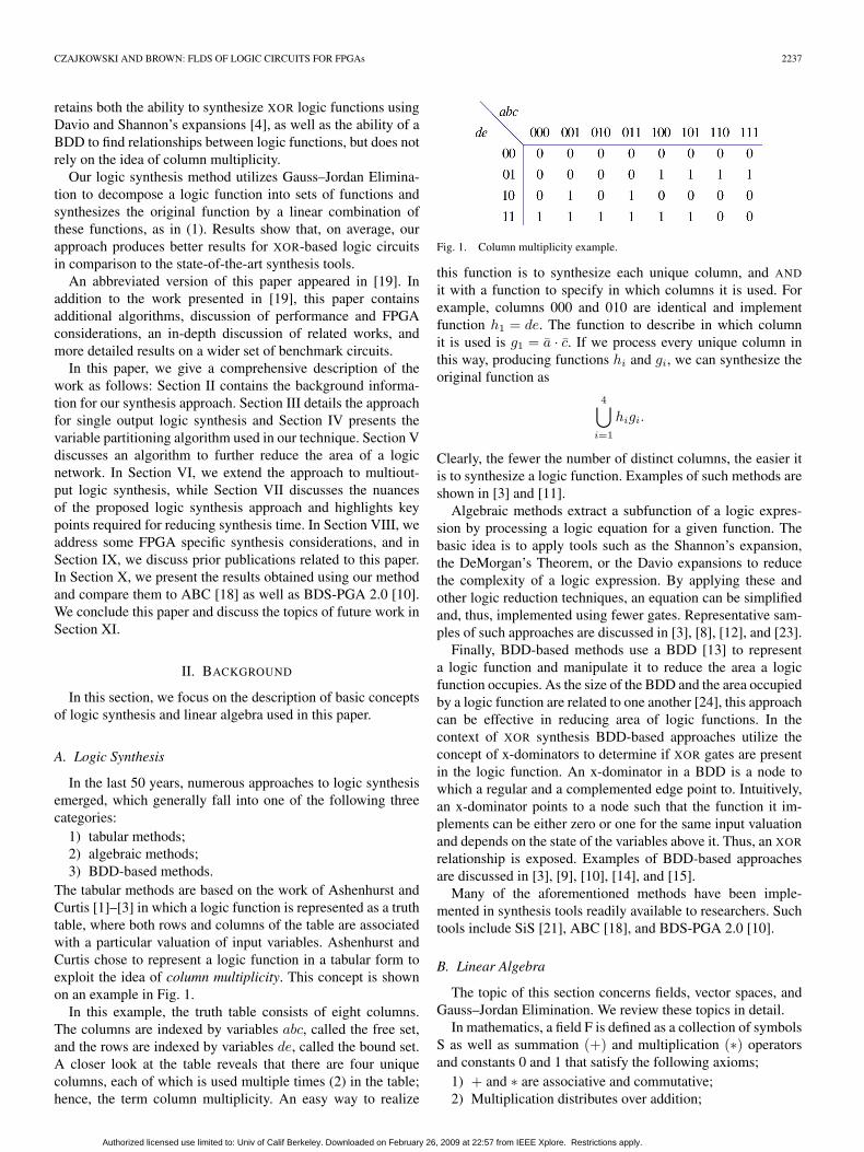
While the set of basis vectors was easy to find in theaforementioned example, a general procedure to find a basisfor any vector space exists. Suppose that we take six vectorsand represent each vector as a column of a matrix [16]
⎡⎢⎣
1 −3 4 −2 5 42 −6 9 −1 8 22 −6 9 −1 9 7−1 3 −4 2 −5 −4
⎤⎥⎦ .
To find a basis for the columns of the matrix, we first applyGaussian Elimination to the matrix.
Gaussian Elimination is a process of applying elementaryrow operations (addition, subtraction and scalar multiplication)to the rows of the matrix to reduce the matrix to an uppertriangular matrix with leftmost elements set to 1. To do this, wefirst pick a row with the nonzero entry in the leftmost column.In this example, let us pick the top row. We then look through allother rows that have a nonzero entry in the same column and tryto make their entries in the same column a zero. To do that, wesubtract a scalar multiple of the top row from a scalar multipleof the other rows. For example, the entry in the first column ofthe second row can be changed to a zero by subtracting twicethe first row from the second. By following this procedure, wereduce the matrix to a row-echelon form [16]:
⎡⎢⎣
1 −3 4 −2 5 40 0 1 3 −2 −60 0 0 0 1 50 0 0 0 0 0
⎤⎥⎦ .
To obtain the basis for the column vectors, we now look at eachnonzero row of the resulting matrix. For each of those rows,the column with the leading 1 corresponds to the column inthe original matrix that is a basis vector for the space spanned
by the column vectors [16]. In this case, these are columns one,three, and five, and therefore, the following are the basis vectorsfor the column vector space:
⎡⎢⎣
122−1
⎤⎥⎦
⎡⎢⎣
499−4
⎤⎥⎦
⎡⎢⎣
589−5
⎤⎥⎦ .
Notice that each column in the original matrix can be repre-sented as a weighted sum of the aforementioned basis vectors.
Gaussian Elimination is sometimes carried out one stepfurther. That is, in addition to reducing the matrix to a row-echelon form, we further reduce the matrix so that the leadingone of each row is the only nonzero entry in the correspondingcolumn. When the procedure is carried out to this point, it isreferred to as Gauss–Jordan Elimination [16], and the resultingmatrix is said to be in the reduced row-echelon form. This isuseful for solving a system of linear equations.
For the purpose of logic synthesis of digital circuits, themathematical operations performed here are in a modulus field,also called a Galois Field. A Galois Field with modulus m isdenoted as GF(m). In particular, we are interested in GF(2),because it facilitates operations on Boolean logic functions. Inthis field, the additive operator is the XOR operation, while alogical AND is equivalent to multiplication.
C. Notations
In the previous sections, we introduced background informa-tion, however, some notation and terms used in logic synthesismay appear to conflict with the well-established norms in linearalgebra. Thus, we explicitly state the notation used throughoutthe remainder of this paper.
In this paper, matrix notation is used with the assumptionthat all operations are performed in GF(2). Thus, summation isequivalent to an XOR operation, and multiplication is equivalentto a logical AND operation. We use ⊕ to represent a sumand a + to represent a logical OR operation. In addition, wewill use ↑ to represent a NAND operation and � to denotean XNOR.
A matrix is denoted by a capital letter, while a columnvector is identified by a lower case bold letter. For example,Ax = b indicates an equation where a matrix A is multipliedby a column vector x, and the result is a column vector b.To distinguish regular column vectors from basis vectors, wedenote basis vectors with bold capital letters. To distinguishinput variables of a logic function from matrices and vectors,input variables of a logic function, as well as the functionoutput, are italicized (e.g., f = abcd).
In this paper, linear algebra is used in the context of logicsynthesis, hence we often represent columns/rows of a matrixas a logic function, rather than as column vectors of 0s and 1s.For example, if a column has four rows, indexed by variablesa and b, then we index the rows from top to bottom as 00, 01,10, and 11. Thus, a statement X = a indicates that the basisvector X is [0011]T, whereas Y = b indicates a basis vector[0101]T.
Authorized licensed use limited to: Univ of Calif Berkeley. Downloaded on February 26, 2009 at 22:57 from IEEE Xplore. Restrictions apply.

CZAJKOWSKI AND BROWN: FLDS OF LOGIC CIRCUITS FOR FPGAs 2239
Fig. 2. Truth Table for Example 1.
Fig. 3. Gaussian Elimination applied to Example 1.
III. BASIC APPROACH
Functionally Linear Decomposition and Synthesis (FLDS) isan approach that exploits an XOR relationship between logicfunctions. It gets its name from the way an XOR relationship isderived, by using the basis of the column space of a truth tableto decompose a function into a set of subfunctions.
The basic idea behind this method is to find subfunctions thatcan be reused in a logic expression and, thus, reduce the sizeof a logic function implementation. It is analogous to Booleanand algebraic division, or kernel extraction. In these methods,we first derive a divisor, or a kernel, and then decompose alogic function with respect to it. In FLDS, we seek to achievea similar effect, however, we take advantage of linear algebrato do it. In our approach, a basis vector is analogous to a“divisor,” and a selector function to specify where a basisvector is used is analogous to a “quotient” from algebraicdivision. The key advantages of our method are the following:a) We can compute basis and selector functions simultaneously;b) the initial synthesis result can easily be optimized using lin-ear algebra; and c) the method is computationally inexpensiveeven for large functions. In this section, we explain the basics ofour approach, and then present methods to refine the synthesisresults in subsequent sections.
Consider a logic function represented by a truth table inFig. 2. The figure shows a truth table for logic function f =ad ⊕ bc, with variables ab at the top and variables cd on theleft-hand side. We will first decompose this function and thensynthesize it.
The first step is to find the basis vectors for the truth tableshown in Fig. 2. To do this, we will apply Gaussian Eliminationto the aforementioned truth table, as though the truth table wasa matrix in GF(2). The procedure, as it is applied to this truthtable, is shown in Fig. 3.
We begin with the initial matrix that directly represents thetruth table and swap the rows, such that the rows are orderedfrom top to bottom based on the column index of their respec-tive leading one entries. The next step is to perform elementaryrow operations to reduce the matrix to the row-echelon form[16]. Thus, we replace row 1 with the sum [XOR in GF(2)] ofrows 0 and 1. This causes row 0 to be the only row with a 1 inthe second column. Finally, we replace row 2 with the sum ofrows 1 and 2, making row 2 consist of all zeros.
In the resulting matrix, the first two rows have leading onesin the middle two columns. From linear algebra [16], we knowthis to indicate that the middle two columns in the original truthtable, or equivalently columns ab = 01 and ab = 10, are thebasis vectors for this function. Therefore, this function has twobasis vectors, G1 = c and G2 = d.
The next step is to express the entire truth table as a linearcombination of these two vectors, which means expressingeach column Ci as h1iG1 ⊕ h2iG2, where h1i and h2i areconstants. To find h1i and h2i, we solve a linear equationAx = b, where A is a matrix formed by basis vectors G1 andG2, x = [h1i h2i]T, and b is the column, we wish to express asa linear combination of basis vectors G1 and G2. For example,to express column C3, we solve the following equation:
⎡⎢⎣
0 00 11 01 1
⎤⎥⎦
[h1i
h2i
]=
⎡⎢⎣
0110
⎤⎥⎦ . (2)
By inspection, the solution to this equation is h1i = 1 andh2i = 1.
We now need to form selector functions that will identifythe columns in which a given basis vector appears. To create aselector function for basis vector G1, we look at the columnsfor which h1 was found to be 1. These columns are ab = 01and ab = 11. Thus, the selector function H1 = b. Similarly, theselector function for G2 is found to be H2 = a. Finally, wecan use (1) to synthesize the function f as H1G1 ⊕ H2G2,producing logic expression f = bc ⊕ ad.
IV. HEURISTIC VARIABLE PARTITIONING
The success of a logic synthesis approach depends heavily onhow variables are chosen during logic decomposition. In fact,by varying the assignment of variables to rows and columnsof a truth table, we can create a table with varying number ofbasis vectors, costs of basis, and selector functions, or both. Theproblem then becomes, as with most synthesis approaches, howto order, or in our case partition, variables. The problem can bedemonstrated on the following example.
Consider the function f = (a � c)(b � d), with variables aand b indexing the columns and c and d indexing the rows,as shown in Fig. 4. By following the procedure outlined inSection III, we find four basis vectors and synthesize it asthe XOR of four minterms. To synthesize the function usingXOR gates efficiently, we need to rearrange variables in thetruth table such that rows, or columns, of the truth table areindexed by variables a and c. Rearranging the variables this
Authorized licensed use limited to: Univ of Calif Berkeley. Downloaded on February 26, 2009 at 22:57 from IEEE Xplore. Restrictions apply.
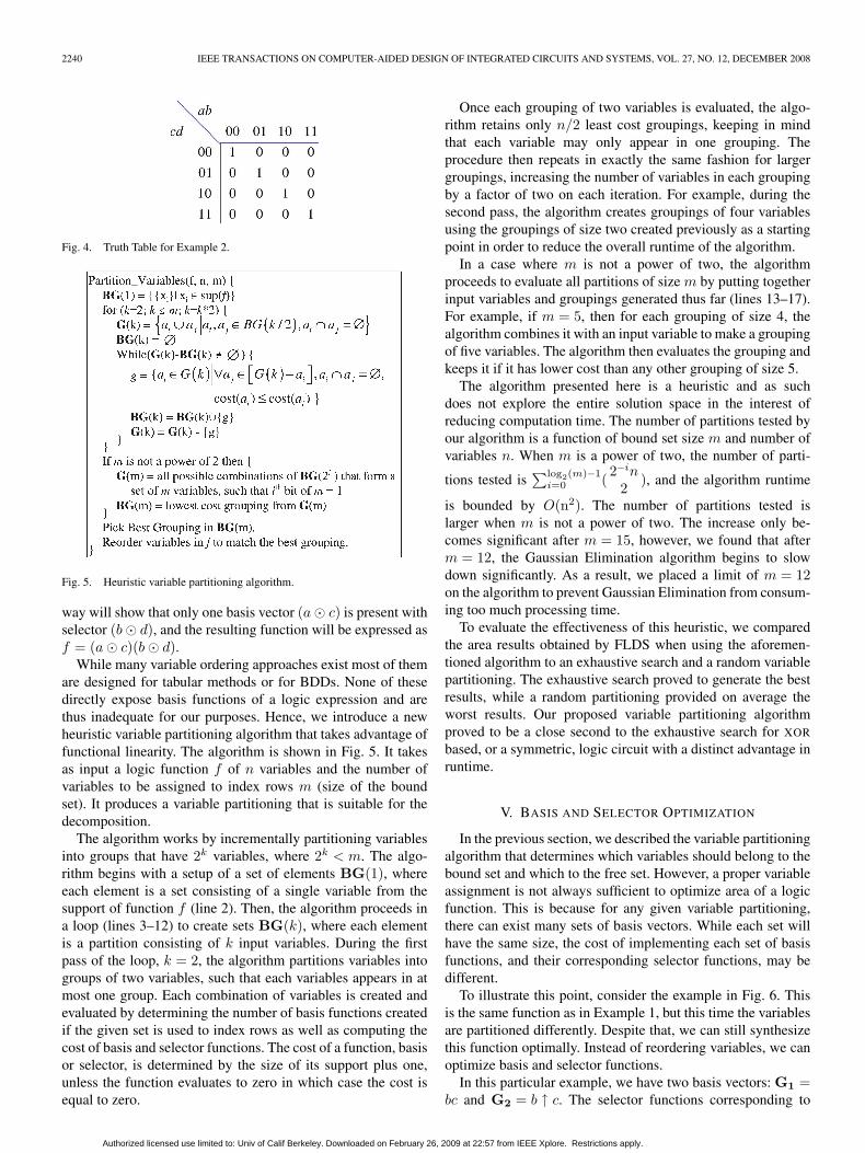
2240 IEEE TRANSACTIONS ON COMPUTER-AIDED DESIGN OF INTEGRATED CIRCUITS AND SYSTEMS, VOL. 27, NO. 12, DECEMBER 2008
Fig. 4. Truth Table for Example 2.
Fig. 5. Heuristic variable partitioning algorithm.
way will show that only one basis vector (a � c) is present withselector (b � d), and the resulting function will be expressed asf = (a � c)(b � d).
While many variable ordering approaches exist most of themare designed for tabular methods or for BDDs. None of thesedirectly expose basis functions of a logic expression and arethus inadequate for our purposes. Hence, we introduce a newheuristic variable partitioning algorithm that takes advantage offunctional linearity. The algorithm is shown in Fig. 5. It takesas input a logic function f of n variables and the number ofvariables to be assigned to index rows m (size of the boundset). It produces a variable partitioning that is suitable for thedecomposition.
The algorithm works by incrementally partitioning variablesinto groups that have 2k variables, where 2k < m. The algo-rithm begins with a setup of a set of elements BG(1), whereeach element is a set consisting of a single variable from thesupport of function f (line 2). Then, the algorithm proceeds ina loop (lines 3–12) to create sets BG(k), where each elementis a partition consisting of k input variables. During the firstpass of the loop, k = 2, the algorithm partitions variables intogroups of two variables, such that each variables appears in atmost one group. Each combination of variables is created andevaluated by determining the number of basis functions createdif the given set is used to index rows as well as computing thecost of basis and selector functions. The cost of a function, basisor selector, is determined by the size of its support plus one,unless the function evaluates to zero in which case the cost isequal to zero.
Once each grouping of two variables is evaluated, the algo-rithm retains only n/2 least cost groupings, keeping in mindthat each variable may only appear in one grouping. Theprocedure then repeats in exactly the same fashion for largergroupings, increasing the number of variables in each groupingby a factor of two on each iteration. For example, during thesecond pass, the algorithm creates groupings of four variablesusing the groupings of size two created previously as a startingpoint in order to reduce the overall runtime of the algorithm.
In a case where m is not a power of two, the algorithmproceeds to evaluate all partitions of size m by putting togetherinput variables and groupings generated thus far (lines 13–17).For example, if m = 5, then for each grouping of size 4, thealgorithm combines it with an input variable to make a groupingof five variables. The algorithm then evaluates the grouping andkeeps it if it has lower cost than any other grouping of size 5.
The algorithm presented here is a heuristic and as suchdoes not explore the entire solution space in the interest ofreducing computation time. The number of partitions tested byour algorithm is a function of bound set size m and number ofvariables n. When m is a power of two, the number of parti-
tions tested is∑log2(m)−1
i=0 ( 2−in2 ), and the algorithm runtime
is bounded by O(n2). The number of partitions tested islarger when m is not a power of two. The increase only be-comes significant after m = 15, however, we found that afterm = 12, the Gaussian Elimination algorithm begins to slowdown significantly. As a result, we placed a limit of m = 12on the algorithm to prevent Gaussian Elimination from consum-ing too much processing time.
To evaluate the effectiveness of this heuristic, we comparedthe area results obtained by FLDS when using the aforemen-tioned algorithm to an exhaustive search and a random variablepartitioning. The exhaustive search proved to generate the bestresults, while a random partitioning provided on average theworst results. Our proposed variable partitioning algorithmproved to be a close second to the exhaustive search for XOR
based, or a symmetric, logic circuit with a distinct advantage inruntime.
V. BASIS AND SELECTOR OPTIMIZATION
In the previous section, we described the variable partitioningalgorithm that determines which variables should belong to thebound set and which to the free set. However, a proper variableassignment is not always sufficient to optimize area of a logicfunction. This is because for any given variable partitioning,there can exist many sets of basis vectors. While each set willhave the same size, the cost of implementing each set of basisfunctions, and their corresponding selector functions, may bedifferent.
To illustrate this point, consider the example in Fig. 6. Thisis the same function as in Example 1, but this time the variablesare partitioned differently. Despite that, we can still synthesizethis function optimally. Instead of reordering variables, we canoptimize basis and selector functions.
In this particular example, we have two basis vectors: G1 =bc and G2 = b ↑ c. The selector functions corresponding to
Authorized licensed use limited to: Univ of Calif Berkeley. Downloaded on February 26, 2009 at 22:57 from IEEE Xplore. Restrictions apply.

CZAJKOWSKI AND BROWN: FLDS OF LOGIC CIRCUITS FOR FPGAs 2241
Fig. 6. Truth Table for Example 3.
Fig. 7. Basis-selector optimization algorithm.
these basis functions are H1 = a ↑ d and H2 = ad. It is pos-sible to replace one of the basis functions with G1 ⊕ G2 andstill have a valid basis function. Notice that G1 ⊕ G2 = 1 and,thus, has a smaller cost than G2 itself. It is therefore better touse G1 ⊕ G2 and G1 to represent the function in Fig. 6. Byinspection, the function f now has basis functions G′
2 = G1 ⊕G2 = 1 and G1 = bc. The corresponding selector functionsare now H ′
2 = ad and H1 = 1. This is because the fourth col-umn of the truth table can now be represented as 1 ⊕ G1 =G2.We can now synthesize function f as f = (H1G1) ⊕(G′
2H ′2) = (bc(1)) ⊕ (ad(1)) = ad ⊕ bc. We obtain the same
result as in Section III.The basis replacement idea is to keep the set of basis func-
tions linearly independent of one another, while reducing thecost of basis and selector functions in the process. Clearly,the basis function pairs {G1,G2}, {G1,G′
2}, {G′2,G2} are
all valid sets of basis functions, as neither element can berepresented as a linear combination of the others. Moreover,each set is capable of expressing each column in the originalmatrix. The only consideration left is how the basis replacementaffects the corresponding selector functions.
A careful analysis reveals that a basis function G2 can bereplaced by G1 ⊕ G2, but it requires the selector function forbasis G1 to be replaced with H1 ⊕ H2. This is because wemust now use basis function G1 wherever G2 was originallyby itself. In addition, wherever G1 and G2 were both used,now only the new basis function G′
2 = G1 ⊕ G2 is used andhence basis function G1 should not be used.
Based on the aforementioned analysis, Fig. 7 shows thebasis–selector optimization algorithm. The algorithm takes asinput the set of basis functions and their corresponding selector
functions and returns a modified set of basis and selectorfunctions. The algorithm works as follows.
First, the algorithm computes the cost of each basis andselector function (line 2). The cost is determined by the supportset size of each function, plus 1, with the exception of afunction equal to zero, for which the cost is zero. The algorithmthen proceeds to evaluate possible improvements to basis andselector functions. This is done by putting together a pair ofbasis–selector function pairs (lines 3–17) to determine if theresulting basis and selector function can replace one of theexisting ones and reduce the basis/selector cost. If replacingan existing basis with a new one does not increase the overallcost of implementing a logic function (lines 9–15), then thealgorithm replaces one of the basis and selector functions.Otherwise, the algorithm attempts to combine a different setof basis and selector functions.
The algorithm iterates until the last three iterations pro-duce the same basis–selector cost, which indicates that fur-ther improvement is unlikely. Note that the algorithm allowsfor basis–selector replacement even if the cost is unchanged,because it may sometimes be necessary to go through a fewintermediate steps before a lower cost basis–selector pair isfound.
When this algorithm is applied to the truth table in Fig. 6, itfinds that using basis function G1 ⊕ G2 = 1, in place of G1 orG2 is preferable. An important point to notice in this exampleis that an all 1s column used does not appear in the truth table inFig. 6. It shows one of the key distinctions between this methodand the classical approach of Ashenhurst and Curtis [1]–[3].
VI. MULTIOUTPUT SYNTHESIS WITH FLDS
The decomposition and synthesis procedure outlined inSection III addresses the issue of synthesizing a single outputlogic function. While it illustrates how the approach generatesa two-level logic network, it is important to extend a synthesistechnique to generate multilevel networks as well as the synthe-sis of logic functions with multiple outputs.
In this section, we discuss two aspects of multilevel andmultioutput function synthesis with FLDS. First, we show howthe function decomposition of a single output function mayresult in a multiple output logic function synthesis. We thenshow how different approaches to multiple output functiondecomposition work in the context of FLDS. Finally, we presenta multioutput synthesis algorithm implement in FLDS.
A. Multilevel Decomposition
A multilevel decomposition of a logic function is neededwhen the final logic expression requires more than two gateson the longest input to output path. In the context of FPGAs,the depth metric is the number of lookup tables (LUTs) on thelongest input to output path. When a logic function has morethan k inputs, it may be necessary for more than 2 k-LUTs tobe created on an input to output path to correctly synthesize afunction.
With FLDS, there are two ways in which this situation canarise. One case is when the number of basis and selector
Authorized licensed use limited to: Univ of Calif Berkeley. Downloaded on February 26, 2009 at 22:57 from IEEE Xplore. Restrictions apply.
2242 IEEE TRANSACTIONS ON COMPUTER-AIDED DESIGN OF INTEGRATED CIRCUITS AND SYSTEMS, VOL. 27, NO. 12, DECEMBER 2008
Fig. 8. Multioutput synthesis example.
functions exceeds k/2, in which case AND/XOR logic createdto combine them will require more than one level of LUTs toimplement. This is not an issue, because the synthesis techniquehas already addressed this by creating the AND/XOR logic, anda function will be synthesized correctly.
The second case is more interesting, and that is when eitherthe basis or the selector function have more than k inputs.Such a case requires further decomposition. It is important tonotice though that in such a case, the variables for the basisfunctions come from a shared set (the selector functions alsoshare variables), which presents an opportunity for further areareduction by extracting their common subfunctions.
B. Multioutput Synthesis
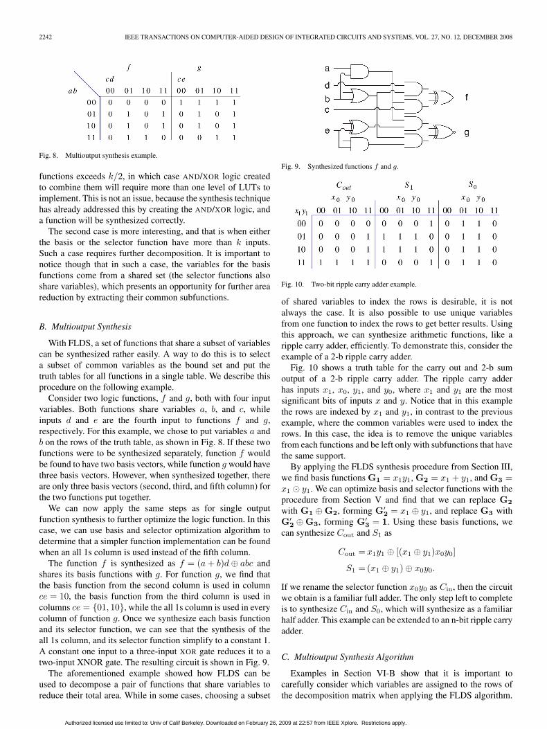
With FLDS, a set of functions that share a subset of variablescan be synthesized rather easily. A way to do this is to selecta subset of common variables as the bound set and put thetruth tables for all functions in a single table. We describe thisprocedure on the following example.
Consider two logic functions, f and g, both with four inputvariables. Both functions share variables a, b, and c, whileinputs d and e are the fourth input to functions f and g,respectively. For this example, we chose to put variables a andb on the rows of the truth table, as shown in Fig. 8. If these twofunctions were to be synthesized separately, function f wouldbe found to have two basis vectors, while function g would havethree basis vectors. However, when synthesized together, thereare only three basis vectors (second, third, and fifth column) forthe two functions put together.
We can now apply the same steps as for single outputfunction synthesis to further optimize the logic function. In thiscase, we can use basis and selector optimization algorithm todetermine that a simpler function implementation can be foundwhen an all 1s column is used instead of the fifth column.
The function f is synthesized as f = (a + b)d ⊕ abc andshares its basis functions with g. For function g, we find thatthe basis function from the second column is used in columnce = 10, the basis function from the third column is used incolumns ce = {01, 10}, while the all 1s column is used in everycolumn of function g. Once we synthesize each basis functionand its selector function, we can see that the synthesis of theall 1s column, and its selector function simplify to a constant 1.A constant one input to a three-input XOR gate reduces it to atwo-input XNOR gate. The resulting circuit is shown in Fig. 9.
The aforementioned example showed how FLDS can beused to decompose a pair of functions that share variables toreduce their total area. While in some cases, choosing a subset
Fig. 9. Synthesized functions f and g.
Fig. 10. Two-bit ripple carry adder example.
of shared variables to index the rows is desirable, it is notalways the case. It is also possible to use unique variablesfrom one function to index the rows to get better results. Usingthis approach, we can synthesize arithmetic functions, like aripple carry adder, efficiently. To demonstrate this, consider theexample of a 2-b ripple carry adder.
Fig. 10 shows a truth table for the carry out and 2-b sumoutput of a 2-b ripple carry adder. The ripple carry adderhas inputs x1, x0, y1, and y0, where x1 and y1 are the mostsignificant bits of inputs x and y. Notice that in this examplethe rows are indexed by x1 and y1, in contrast to the previousexample, where the common variables were used to index therows. In this case, the idea is to remove the unique variablesfrom each functions and be left only with subfunctions that havethe same support.
By applying the FLDS synthesis procedure from Section III,we find basis functions G1 = x1y1, G2 = x1 + y1, and G3 =x1 � y1. We can optimize basis and selector functions with theprocedure from Section V and find that we can replace G2
with G1 ⊕ G2, forming G′2 = x1 ⊕ y1, and replace G3 with
G′2 ⊕ G3, forming G′
3 = 1. Using these basis functions, wecan synthesize Cout and S1 as
Cout = x1y1 ⊕ [(x1 ⊕ y1)x0y0]
S1 = (x1 ⊕ y1) ⊕ x0y0.
If we rename the selector function x0y0 as Cin, then the circuitwe obtain is a familiar full adder. The only step left to completeis to synthesize Cin and S0, which will synthesize as a familiarhalf adder. This example can be extended to an n-bit ripple carryadder.
C. Multioutput Synthesis Algorithm
Examples in Section VI-B show that it is important tocarefully consider which variables are assigned to the rows ofthe decomposition matrix when applying the FLDS algorithm.
Authorized licensed use limited to: Univ of Calif Berkeley. Downloaded on February 26, 2009 at 22:57 from IEEE Xplore. Restrictions apply.
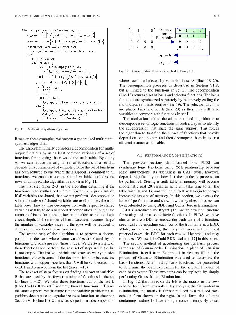
CZAJKOWSKI AND BROWN: FLDS OF LOGIC CIRCUITS FOR FPGAs 2243
Fig. 11. Multioutput synthesis algorithm.
Based on these examples, we present a generalized multioutputsynthesis algorithm.
The algorithm initially considers a decomposition for multi-output functions by using least common variables of a set offunctions for indexing the rows of the truth table. By doingso, we can reduce the original set of functions to a set thatdepends on a common set of variables. Once the set of functionshas been reduced to one where their support is common to allfunctions, we can then use the shared variables to index therows of a matrix. The algorithm is shown in Fig. 11.
The first step (lines 2–3) in the algorithm determine if thefunctions to be synthesized share all variables, or just a subset.If all variables are shared, then we can perform a decompositionwhere the subset of shared variables are used to index the truthtable rows (line 5). The decomposition with respect to sharedvariables will try to do a balanced decomposition so long as thenumber of basis functions is low in an effort to reduce logiccircuit depth. If the number of basis functions becomes large,the number of variables indexing the rows will be reduced todecrease the number of basis functions.
The second step of the algorithm is to perform a decom-position in the case where some variables are shared by allfunctions and some are not (lines 7–22). We create a list L ofthese functions and perform the next set of steps while the listis not empty. The list will shrink and grow as we synthesizefunctions, either because of the decomposition, or because thefunctions with support size less than k will be synthesized intok-LUT and removed from the list (lines 9–10).
The next set of steps focuses on finding a subset of variablesS that are used by the fewest number of functions in the setL (lines 11–12). We take these functions out of the set L(lines 13–14). If the set L is empty, then all functions in F havethe same support. We therefore run the variable partitioning al-gorithm, decompose and synthesize these functions as shown inSection VI-B (line 16). Otherwise, we perform a decomposition
Fig. 12. Gauss–Jordan Elimination applied to Example 1.
where rows are indexed by variables in set S (lines 18–20).The decomposition proceeds as described in Section VI-B,but is limited to the functions in set F. The decomposition(line 18) returns a set of basis and selector functions. The basisfunctions are synthesized separately by recursively calling themultioutput synthesis routine (line 19). The selector functionsare placed back into set L (line 20) as they may still havevariables in common with functions in set L.
The motivation behind the aforementioned algorithm is todecompose a set of logic functions in such a way as to identifythe subexpression that share the same support. This forcesthe algorithm to first find the subset of functions that heavilydepend on one another, and then decompose them in as areaefficient manner as it is able.
VII. PERFORMANCE CONSIDERATIONS
The previous sections demonstrated how FLDS cansynthesize logic functions using XOR relationship betweenlogic subfunctions. Its usefulness in CAD tools, however,depends significantly on how fast the synthesis process canbe performed. Storing a truth table in memory will becomeproblematic past 20 variables as it will take time to fill thetable with 0s and 1s, and the table itself will begin to occupyincreasing amount of memory. In this section, we discuss theissue of performance and show how the synthesis process canbe accelerated by using BDDs and Gauss–Jordan Elimination.
BDDs introduced by Bryant [13] are an efficient structurefor storing and processing logic functions. In FLDS, we havechosen to use BDDs to encode the truth table of a function,specifically by encoding each row of the truth table as a BDD.While, in extreme cases, this may not work well, in mostpractical cases, the BDD for each row will be small and easyto process. We used the Cudd BDD package [17] in this paper.
The second method of accelerating the synthesis processis the use of Gauss–Jordan Elimination in place of GaussianElimination. Recall from Example 1 in Section III that theprocess of Gaussian Elimination was used to determine thebasis functions. After finding basis functions, we proceededto determine the logic expression for the selector function ofeach basis vector. These two steps can be replaced by simplyperforming Gauss–Jordan Elimination.
In Fig. 12, the matrix on the left is the matrix in the row-echelon form from Example 1. By applying the Gauss–JordanElimination, the matrix is further reduced to a reduced row-echelon form shown on the right. In this form, the columnscontaining leading 1s have a single nonzero entry. By closer
Authorized licensed use limited to: Univ of Calif Berkeley. Downloaded on February 26, 2009 at 22:57 from IEEE Xplore. Restrictions apply.

2244 IEEE TRANSACTIONS ON COMPUTER-AIDED DESIGN OF INTEGRATED CIRCUITS AND SYSTEMS, VOL. 27, NO. 12, DECEMBER 2008
inspection, we can see that the first row in the reduced row-echelon form matrix corresponds to the truth table of theselector function for the first basis vector. Similarly, the secondrow of this matrix corresponds to the selector function for thesecond basis vector.
Notice that in Section III, we found the equations for H1
and H2 by solving linear equations for each column of thetruth table. Gauss–Jordan Elimination solves this problem forus. This is a property of the Gauss–Jordan Elimination [16],and while it is useful in solving linear equation, it is shownhere that it is also important in the context of logic synthesisas the columns of the matrix are related by variables used toindex them. Hence, the selector functions can be computedrapidly.
VIII. FPGA CONSIDERATIONS
In the previous sections, synthesis and processing time issueswere addressed by using algebraic manipulation. The aboveneed to be augmented by considering the target platform forsynthesis, which in our case are FPGAs.
In particular, a key parameter is the size of a LUT, k, usedby an FPGA. The idea here is that the decomposition processshould take into consideration the amount of space basis andselector functions will take. In our implementation, any func-tion of k or fewer variables is synthesized into a single LUT.This presents an opportunity for area recovery as it is possiblefor the same function to be synthesized multiple times. Thiscan either happen by synthesizing two functions in tandem, orone after another. As such, it is important to recognize repeatedfunctionality and reuse it. For this purpose, we use a hashtable of logic functions of k and fewer inputs. Every time aLUT is synthesized, it is put in a hash table, using the set ofinput variables key entries. If another LUT is to be created, wefirst check if the LUT function, or its complement, has alreadybeen synthesized. If so, rather than creating a new LUT, a wireor an inverter connection is added to the logic graph therebysaving area.
Another consideration is that modern FPGAs contain morecomplex logic than simple LUTs and FFs. In fact, both Alteraand Xilinx FPGAs contain carry chains to implement fast ripplecarry adders. Because these adders contain XOR gates outsideof the LUT network, it is possible to utilize these XOR gates tofurther reduce the area taken by a logic function. This, however,is a topic for future work.
IX. RELATED WORK
FLDS resembles tabular methods based on the work ofAshenhurst and Curtis [1]–[3]. However, there are key differ-ences between these methods and FLDS.
The tabular method looks for column multiplicity in a truthtable, hoping to exploit it in an effort to reduce circuit area. Inthe example in Fig. 1, we found four distinct columns usingthe tabular method, but by inspection, we can see that FLDSfinds three basis functions for this truth table. A second differ-ence between the tabular method and FLDS was illustrated inExample 3 in Section IV. Specifically, we showed that during
Fig. 13. XOR gate replacement example.
Fig. 14. Example of XOR gate replacement.
the synthesis, FLDS can utilize columns that do not actuallyappear in the truth table to reduce circuit area.
In a special case, FLDS simplifies to the tabular method. Anexample of such a case is the synthesis of a wide AND gate (e.g.,f = abcde). In this particular case, we find that the number ofdistinct columns and the number of basis vectors are the same.In more general terms, FLDS reduces to the tabular method ifone of the following is true:
1) The product of all pairs of selector functions is zero.2) The product of all pairs of basis functions is zero.
The aforementioned relationship between FLDS and thetabular method can be exploited in non-FPGA context, whereit may be advantageous to replace XOR gates with OR gates. InFLDS, it is easy to determine if an XOR gate can be replaced byan OR gate. If a product of a pair of basis functions, or theirrespective selector functions, is equal to zero, then the XOR
gate used to sum the basis–selector products for this pair ofsubfunctions can be replaced by an OR gate. An example isgiven below.
Fig. 13 shows a logic function with three basis functions.They are G1 = c, G2 = d, and G3 = 1. We can see that G1
is used in columns ab = 00 and 10, G2 is used in columnsab = 01 and 11, while G3 is used in columns ab = 10 and 11.Using only two-input gates, this function can be realized, asshown in Fig. 14(a). Notice however that the selector functionsfor G1 and G2 are complements of one another, and thus, theirproduct is equal to zero. It is therefore unnecessary to sum thesetwo subfunctions using an XOR gate. An OR gate can be usedinstead to implement the same logic expression. This is shownin Fig. 14(b).
Positive and negative Davio expansions, useful for XOR
decomposition, are also a special case of FLDS. To derive themusing FLDS, assign a single variable x to the bound set. Thiswill result in two basis and selector functions, and the functionf can be synthesized as follows:
f = xfx ⊕ xfx. (3)
Authorized licensed use limited to: Univ of Calif Berkeley. Downloaded on February 26, 2009 at 22:57 from IEEE Xplore. Restrictions apply.

CZAJKOWSKI AND BROWN: FLDS OF LOGIC CIRCUITS FOR FPGAs 2245
By replacing one of the basis functions with x ⊕ x = 1, weproduce one of the following equations:
f = fx ⊕ x(fx ⊕ fx) (4)
f = (fx ⊕ fx)x ⊕ fx. (5)
Equations (4) and (5) are the negative and the positive DavioExpansions, respectively.
The consequence of the ability to decompose a logic functionusing (3)–(5) using a cost function is the ability to synthesizeexclusive OR sum of products expressions of various classes. Inparticular, if FLDS is set up to decompose a logic function onevariable at a time, it will generate either a Pseudo Kroneckerexpression or Generalized Reed–Muller expression for a logicfunction [4]. The choice of the expression generated dependson the cost of implementing the basis and selector functions.If during the decomposition (3)–(5) are used, then a PseudoKronecker expression will be formed. However, if the expan-sion is carried out using only (4) and (5), then the resultingexpression will be in a Generalized Reed–Muller form. Thechoice between the two forms depends on which option pro-duces basis and selector functions of lower cost.
Another work closely related to FLDS is called Factor [20].Factor is an approach to logic decomposition based on SingleValue Decomposition (SVD). FLDS differs from factor inseveral ways.
The first difference between the two approaches is the useof basis and selector optimization algorithm in FLDS. Thisalgorithm, as shown in Section V, provides the means to furtherreduce the cost of logic implementation, even if the initial set ofbasis functions is minimal. This is not the case with factor. Infact, Factor requires not only a good variable partitioning, butalso a good variable ordering within each partition to achieve agood result, because it does not use an algorithm similar to thebasis and selector optimization.
The second difference is that the work in [20] can onlyperform a balanced decomposition. As we have shown earlier,FLDS is not limited to performing a balanced decomposition.In that respect, this paper generalizes the approach in [20] tocover both balanced and unbalanced decompositions.
The third difference is that the decomposition in [20] uses analgorithm of the same runtime as Gaussian Elimination severaltimes to perform the decomposition of a single function. Thegoal there is to find logic expressions for each subfunction.In FLDS, we use Gauss–Jordan Elimination to achieve thesame goal faster. The advantage here is that Gauss–JordanElimination requires the use of row operations only. This factis used to set up data structures in an efficient manner, allowingfor a fast processing time.
The fourth difference is in how FLDS and [20] handlemultioutput logic functions. In [20], the decomposition canresult in a linear dependence of logic subfunctions, because thealgorithm picks a variable partition that minimizes the rank ofeach individual logic function, but it does not remove the lineardependencies between the generated logic subfunctions. Thus,a subset of functions generated by the decomposition in [20] fortwo functions f and g may be such that the subfunctions of fare linearly dependent on subfunctions of g.
Fig. 15. Example of the differences between FLDS and Factor.
This is not the case with FLDS. FLDS addresses bothlinear dependence and subfunction minimization of multipleoutput functions. First, we generate linearly independent set ofsubfunctions for all selected functions. Any linear dependen-cies between the subfunctions are removed by using GaussianElimination. Second, a basis and selector function optimizationalgorithm, which runs in O(n2) for n basis vectors, does agood job at finding lower cost subfunctions. As demonstratedin Section V, this helps us reduce logic area. To illustrate thesedifferences, consider the following example.
Fig. 15 shows two functions f and g as they are representedby FLDS and factor [20]. During synthesis, the algorithm pre-sented by Hwang et al. [20] uses the setup shown on the right-hand side of Fig. 15 to decompose the logic functions f and ginto subfunctions G1 = a and G2 = b for f and G3 = a ⊕ band G1 = a for g. However, the algorithm does not exploitthe relationship G3 = G1 ⊕ G2 to reduce logic area and, as aconsequence, synthesizes functions f and g using a total of sixtwo-input gates. In contrast, FLDS optimizes G3 away becauseof a linear dependence on G1 and G2. FLDS decomposes bothf and g with respect to G1 and G2, synthesizing the circuitusing only four two-input gates.
Finally, our approach uses a fast variable partitioning ap-proach, whereas the work in [20] does not. A follow up workin [22] uses cubical notation to perform analysis of a logicfunction to better choose variable partitioning for the algorithmin [20]. However, the number of cubes can be quite large andthe approach is only viable for small logic functions.
X. EXPERIMENTAL RESULTS
In this section, we present area, depth, and compilationtime results and compare them to previously published works.The following sections contain the experimental methodology,summary of results, and discussion.
A. Methodology
In this paper, the area results obtained from FLDS were com-pared to two academic synthesis systems: ABC [18] optimizes acircuit using structural transformations, and BDS-PGA 2.0 [10]performs Boolean optimization by utilizing BDDs.
To obtain results using ABC, each circuit was first convertedto an AND-Inverter Graph (AIG) using the strash command.The circuit was then optimized using the resyn2 script thatoperates on AIGs to reduce the circuit size, and the resulting
Authorized licensed use limited to: Univ of Calif Berkeley. Downloaded on February 26, 2009 at 22:57 from IEEE Xplore. Restrictions apply.
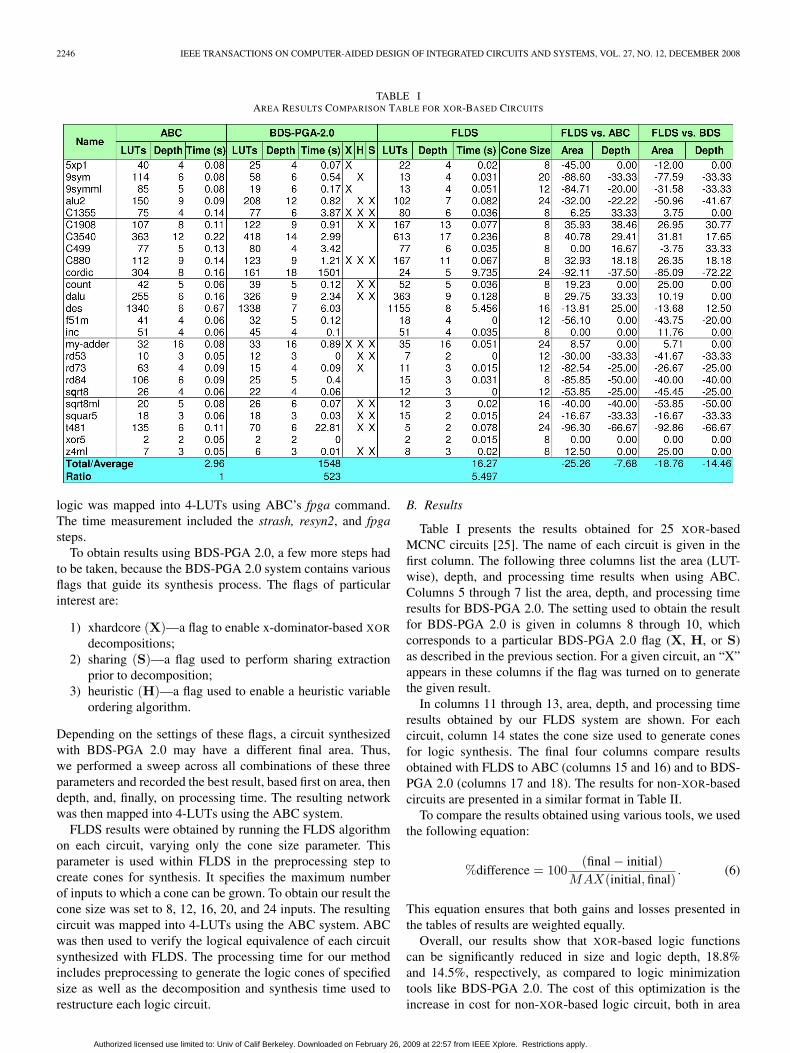
2246 IEEE TRANSACTIONS ON COMPUTER-AIDED DESIGN OF INTEGRATED CIRCUITS AND SYSTEMS, VOL. 27, NO. 12, DECEMBER 2008
TABLE IAREA RESULTS COMPARISON TABLE FOR XOR-BASED CIRCUITS
logic was mapped into 4-LUTs using ABC’s fpga command.The time measurement included the strash, resyn2, and fpgasteps.
To obtain results using BDS-PGA 2.0, a few more steps hadto be taken, because the BDS-PGA 2.0 system contains variousflags that guide its synthesis process. The flags of particularinterest are:
1) xhardcore (X)—a flag to enable x-dominator-based XOR
decompositions;2) sharing (S)—a flag used to perform sharing extraction
prior to decomposition;3) heuristic (H)—a flag used to enable a heuristic variable
ordering algorithm.
Depending on the settings of these flags, a circuit synthesizedwith BDS-PGA 2.0 may have a different final area. Thus,we performed a sweep across all combinations of these threeparameters and recorded the best result, based first on area, thendepth, and, finally, on processing time. The resulting networkwas then mapped into 4-LUTs using the ABC system.
FLDS results were obtained by running the FLDS algorithmon each circuit, varying only the cone size parameter. Thisparameter is used within FLDS in the preprocessing step tocreate cones for synthesis. It specifies the maximum numberof inputs to which a cone can be grown. To obtain our result thecone size was set to 8, 12, 16, 20, and 24 inputs. The resultingcircuit was mapped into 4-LUTs using the ABC system. ABCwas then used to verify the logical equivalence of each circuitsynthesized with FLDS. The processing time for our methodincludes preprocessing to generate the logic cones of specifiedsize as well as the decomposition and synthesis time used torestructure each logic circuit.
B. Results
Table I presents the results obtained for 25 XOR-basedMCNC circuits [25]. The name of each circuit is given in thefirst column. The following three columns list the area (LUT-wise), depth, and processing time results when using ABC.Columns 5 through 7 list the area, depth, and processing timeresults for BDS-PGA 2.0. The setting used to obtain the resultfor BDS-PGA 2.0 is given in columns 8 through 10, whichcorresponds to a particular BDS-PGA 2.0 flag (X, H, or S)as described in the previous section. For a given circuit, an “X”appears in these columns if the flag was turned on to generatethe given result.
In columns 11 through 13, area, depth, and processing timeresults obtained by our FLDS system are shown. For eachcircuit, column 14 states the cone size used to generate conesfor logic synthesis. The final four columns compare resultsobtained with FLDS to ABC (columns 15 and 16) and to BDS-PGA 2.0 (columns 17 and 18). The results for non-XOR-basedcircuits are presented in a similar format in Table II.
To compare the results obtained using various tools, we usedthe following equation:
%difference = 100(final − initial)
MAX(initial, final). (6)
This equation ensures that both gains and losses presented inthe tables of results are weighted equally.
Overall, our results show that XOR-based logic functionscan be significantly reduced in size and logic depth, 18.8%and 14.5%, respectively, as compared to logic minimizationtools like BDS-PGA 2.0. The cost of this optimization is theincrease in cost for non-XOR-based logic circuit, both in area
Authorized licensed use limited to: Univ of Calif Berkeley. Downloaded on February 26, 2009 at 22:57 from IEEE Xplore. Restrictions apply.

CZAJKOWSKI AND BROWN: FLDS OF LOGIC CIRCUITS FOR FPGAs 2247
TABLE IIAREA RESULTS FOR NON-XOR-BASED LOGIC CIRCUITS
Authorized licensed use limited to: Univ of Calif Berkeley. Downloaded on February 26, 2009 at 22:57 from IEEE Xplore. Restrictions apply.

2248 IEEE TRANSACTIONS ON COMPUTER-AIDED DESIGN OF INTEGRATED CIRCUITS AND SYSTEMS, VOL. 27, NO. 12, DECEMBER 2008
and in depth by 4.8% and 6.2%, respectively. As compared tostructural optimization techniques, such as those used in ABC,FLDS synthesizes XOR-based circuits using 25.3% less areaand reduces logic depth by 7.7%. For non-XOR-based logiccircuits, ABC produces circuits with 6.2% lower area resultsand 16.5% lower depth on average than FLDS.
C. Discussion of Individual Circuits
As shown in Table I, significant area savings are found usingFLDS. The largest area savings for XOR-based circuits wereobserved for 9sym, cordic, sqrt8ml, and t481.
9sym is a circuit with a single nine input logic function.The circuit itself consists of a number of XOR gates. Inter-estingly enough, 9symml represents the same function, exceptwith a different initial representation, was synthesized muchbetter than 9sym. In 9sym, BDS-PGA 2.0 found the circuit toconsist of nine logic functions and hence was unable to finda compact implementation for it, although it faired 30% betterthan ABC. However, for 9symml, BDS-PGA found it to be asingle output nine-input function and created a single BDD forit. Despite finding a single cone of logic for 9symml, BDS-PGAproduced a 30% worse result than FLDS. This example showsthat functionally linear decomposition and x-dominator-baseddecompositions are quite different. While both strive to utilizeXOR gates, searching for an x-dominator in a BDD clearly doesnot guarantee finding a better decomposition.
Another interesting circuit is cordic. It consists of two func-tions sharing 23 inputs. In this particular case, the results weobtained come from two sources: the ability to synthesizelarge functions and synthesizing multioutput functions. FLDSfound the functions to be reasonably easy to synthesize using abalanced decomposition.
In contrast, neither ABC nor BDS-PGA found there to beonly two cones of logic. Instead, many cones were createdto represent this circuit. In the case of BDS-PGA, 32 logicfunctions were created. While in Table I, the synthesis flags forthis circuit do not include x-dominator decompositions usage,the results with the same flag turned on were identical, exceptfor the longer processing time.
Sqrt8ml is an arithmetic circuit that computes a square rootof a binary number. It consists of four logic functions, with two,four, six, and eight inputs. The two functions that fit in a singleLUT were synthesized separately, but the six and eight inputfunctions were synthesized in tandem. The algorithm found fivebasis vectors shared by these two functions. In the worst casescenario, this would cause 15 LUTs to be created to implementthese two functions, but due to our basis and selector functionoptimization routine, this was not the case. Specifically, thebasis and selector function optimization led to the realizationof the basis and selector functions using fewer variables. Thus,the mapping stage of the CAD flow could successfully mapboth functions into a total of ten LUTs. The result we obtainedwas nearly half the size of the one produced by ABC, and lessthan half of the area taken by the same circuit synthesized withBDS-PGA.
The t481 circuit is a 16-input single-output logic func-tion, which has a compact representation in the Fixed-Polarity
Fig. 16. Distribution of area savings compared to ABC.
Reed–Muller form. When synthesized correctly, it takes onlyfive four-LUTs, which is the minimum for this circuit. In FLDS,the function was synthesized in 0.125 s, finding only two basisfunctions during balanced decomposition. In this particularcase, the variable partitioning algorithm was successful infinding the correct assignment of variables to the bound andthe free set, which allowed for minimum area synthesis of thelogic function.
The success of our method is not limited to XOR-basedlogic functions. Table II shows the results for non-XOR-basedlogic circuits from the MCNC benchmark set. The columns inTable II have the same meaning as in Table I. As shown inthe table, numerous logic circuits that are considered not tobe XOR-based have benefited significantly as well. Examplesof such circuits are ex5p, pdc, sao2, and ex1010.1 In thesecircuits, pdc and ex1010 in particular, the success is attributedto synthesis of multioutput functions, rather than synthesizingeach cone of logic separately. The pdc circuit did take FLDS2.5 times longer to synthesize than when using BDS-PGA 2.0,but the achieved result is nearly six times smaller and with a30% lower logic depth.
The results produced by FLDS can be further improved byapplying existing logic synthesis techniques on top of FLDS.In this paper, we investigated the effect of applying the resyn2script of ABC on top of FLDS results to determine if it canfurther reduce logic area. We found that if ABC is used ontop of FLDS and the results compared to those obtained usingABC alone for the same set of circuits, then we obtain a 24.2%smaller area and a 16.2% lower depth for XOR-based circuits.For non-XOR-based circuits area was 4.25% smaller with onlya 1% depth increase. Averaged over both XOR-based and non-XOR-based circuits, FLDS together with ABC can reduce anaverage circuit size by 9.3% and reduce the depth by 3.3%, ascompared to what ABC can do alone. The distribution of resultsis shown in Fig. 16.
XI. CONCLUSION
The FLDS technique was found to be very effective inreducing area taken by logic functions heavily dependent onXOR gates. It achieved a 25% reduction in area as compared
1This circuit failed to synthesize with BDS-PGA 2.0 and, hence, is excludedfrom average/total computation. FLDS produced a result in 13.94 s, resulting in1063 LUTs and a depth of seven. In contrast, ABC produced a result in 1.52 scontaining 4094 LUTs with depth eight.
Authorized licensed use limited to: Univ of Calif Berkeley. Downloaded on February 26, 2009 at 22:57 from IEEE Xplore. Restrictions apply.
CZAJKOWSKI AND BROWN: FLDS OF LOGIC CIRCUITS FOR FPGAs 2249
to ABC [18], as well as an 18.8% reduction in comparison toBDD-based approaches used in BDS-PGA 2.0 [10]. We alsoshowed that FLDS provides a depth reduction of 7.7% and14.48%, respectively, compared to these approaches. For non-XOR intensive logic circuits, the technique suffers only a minorarea and depth penalty. For both of these groups of functions,FLDS performed synthesis rapidly.
The technique presented here can be further improved. In theshort term, the most promising is the extension of this techniqueto cover nondisjoint decompositions. A challenge here willbe to modify the variable partitioning technique to select thecorrect variables to overlap between the bound and the free sets.
Another extension to consider is to apply the proposedapproach to multivalued logic decompositions. Since this ap-proach is quite generic in terms of the underlying mathematicalfield used, it will be valid for any valid GF(m). However, theaddition, subtraction, and multiplication operations may provemore complex for m > 2, mostly because the final implemen-tation is in terms of Boolean logic.
ACKNOWLEDGMENT
The authors would like to thank Dr. D. Singh andDr. V. Manohararajah from Altera Corporation for suggestionsduring the course of this paper. The authors would also like tothank Prof. Z. G. Vranesic and Prof. J. Zhu from the Universityof Toronto for their feedback throughout the course of thispaper.
REFERENCES
[1] R. L. Ashenhurst, “The decomposition of switching functions,” in Proc.Int. Symp. Theory Switching, Apr. 2–5, 1957, pp. 74–116.
[2] H. A. Curtis, A New Approach to the Design of Switching Circuits.Princeton, NJ: Van Nostrand, 1962.
[3] M. Perkowski and S. Grygiel, “A survey of literature on function de-composition,” in “A Final Report for Summer Faculty Research Program,Wright Laboratory,” Air Force Office Sci. Res., Bolling Air Force Base,Wright Lab., Washington, DC, Sep. 1994.
[4] T. Sasao, Switching Theory for Logic Synthesis. Norwell, MA: Kluwer,1999.
[5] S. L. Hurst, D. M. Miller, and J. C. Muzio, Spectral Techniques in DigitalLogic. London, U.K.: Academic, 1985.
[6] E. M. Clarke, K. McMillan, X. Zhao, M. Fujita, and J. Yang, “Spectraltransforms for large Boolean functions with applications to technologymapping,” in Proc. 30th DAC, Jun. 1993, pp. 54–60.
[7] M. G. Karpovsky, “Harmonic analysis over finite commutative groupsin linearization problems for systems of logical functions,” Inf. Control,vol. 33, no. 2, pp. 142–165, Feb. 1977.
[8] C. Tsai and M. Marek-Sadowska, “Multilevel logic synthesis forarithmetic functions,” in Proc. 33rd DAC, Jun. 1996, pp. 242–247.
[9] C. Yang, M. Ciesielski, and V. Singhal, “BDS: A BDD-based logicoptimization system,” in Proc. 37th ICCAD, 2000, pp. 92–97.
[10] N. Vemuri, P. Kalla, and R. Tessier, “BDD-based logic synthesis forLUT-based FPGAs,” ACM Trans. Des. Autom. Electron. Devices, vol. 7,no. 4, pp. 501–525, Oct. 2002.
[11] W. Wan and M. A. Perkowski, “A new approach to the decompositionof incompletely specified multi-output functions based on graph coloringand local transformations and its application to FPGA mapping,” in Proc.Eur. Des. Autom. Conf., 1992, pp. 230–235.
[12] T. Sasao and J. T. Butler, “A design method for look-up table type FPGAby pseudo-Kronecker expansion,” in Proc. 24th Int. Symp. Multi-ValuedLogic, 1994, pp. 97–106.
[13] R. E. Bryant, “Graph-based algorithms for Boolean function manipula-tion,” IEEE Trans. Comput., vol. C-35, no. 8, pp. 677–691, Aug. 1986.
[14] Y. T. Lai, M. Pedram, and S. Sastry, “BDD based decomposition of logicfunctions with application to FPGA synthesis,” in Proc. 30th Des. Autom.Conf., 1993, pp. 642–647.
[15] C. Yang, V. Singhal, and M. Ciesielski, “BDD decomposition for efficientlogic synthesis,” in Proc. Int. Conf. Comput. Des., 1999, pp. 626–631.
[16] H. Anton and C. Rorres, Elementary Linear Algebra, ApplicationsVersion, 7th ed. Hoboken, NJ: Wiley, 1994.
[17] F. Somenzi, CUDD: CU Decision Diagram Package, Release 2.4.1.[Online]. Available: http://vlsi.colorado.edu/~fabio/CUDD
[18] Berkeley Logic Synthesis Group, ABC: A System for Sequential Syn-thesis and Verification, Dec. 2005. [Online]. Available: http://www.eecs.berkeley.edu/~alanmi/abc
[19] T. S. Czajkowski and S. D. Brown, “Functionally linear decompositionand synthesis of logic circuits for FPGAs,” in Proc. IEEE 45th DAC,Jun. 2008, pp. 18–23.
[20] T. T Hwang, R. M. Owens, and M. J. Irwin, “Exploiting communicationcomplexity for multilevel logic synthesis,” IEEE Trans. Comput.-AidedDesign Integr. Circuits Syst., vol. 9, no. 10, pp. 1017–1027, Oct. 1990.
[21] E. M. Sentovich, K. J. Singh, L. Lavagno, C. Moon, R. Murgai,A. Saldanha, H. Savoj, P. R. Stephan, R. K. Brayton, and A. Sangiovanni-Vincentelli, SIS: A System for Sequential Circuit Synthesis. Berkeley,CA: Dept. EECS, Univ. California, 1992.
[22] T. T Hwang, R. M. Owens, and M. J. Irwin, “Efficiently computingcommunication complexity for multilevel logic synthesis,” IEEE Trans.Comput.-Aided Design Integr. Circuits Syst., vol. 11, no. 5, pp. 545–554,May 1992.
[23] A. Bernasconi, V. Ciriani, and R. Cordone, “The optimization of kEP-SOPs: Computational complexity, approximability and experiments,”ACM Trans. Des. Autom. Electron. Syst., vol. 13, no. 2, pp. 1–31, 2008.art. no. 35.
[24] C. L. Berman, “Ordered binary decision diagrams and circuit structure,”in Proc. IEEE Int. Conf. Comput. Des., Cambridge, MA, Oct. 1989,pp. 392–395.
[25] S. Yang, “Logic synthesis and optimization benchmarks User Guide 3.0,”Microelectron. Center North Carolina, Research Triangle Park, NC, 1991.Tech. Rep.
Tomasz S. Czajkowski (M’02) received theB.A.Sc., M.A.Sc., and Ph.D. (exploring a relativelyrecent approach to field-programmable gate array(FPGA) computer-aided design flow called physicalsynthesis) degrees from the Department of Electricaland Computer Engineering, University of Toronto,Toronto, ON, Canada, in 2001, 2004, and 2008,respectively.
He is currently with the University of Toronto.His work focused on logic implementation and opti-mization of circuits as it pertains to FPGA devices,
looking in particular at how various logic structures can be utilized moreeffectively. In this context, he is mostly interested in the synthesis and physicalimplementation of logic circuits, taking into account logic structures availableon FPGAs, circuit performance, area, and power dissipation.
Stephen D. Brown (M’89) received the Ph.D. andM.A.Sc. degrees in electrical engineering from theUniversity of Toronto, Toronto, ON, Canada, andthe B.A.Sc. degree in electrical engineering fromthe University of New Brunswick, Fredericton, NB,Canada.
He was with the University of Toronto faculty in1992, where he currently holds the rank of Professorwith the Department of Electrical and ComputerEngineering. He also holds the position of Architectwith the Altera Toronto Technology Centre, Toronto,
a world-leading research and development site for computer-aided design(CAD) software and field-programmable gate array architectures, where heis involved in research activities and is the Director of the Altera UniversityProgram. His research interests include field-programmable very large scaleintegration technology, CAD algorithms, and computer architecture. He isa coauthor of more than 60 scientific research papers and three textbooks:Fundamentals of Digital Logic with Verilog Design, Fundamentals of DigitalLogic with VHDL Design, and Field-Programmable Gate Arrays.
Dr. Brown won the Canadian Natural Sciences and Engineering ResearchCouncils 1992 Doctoral Prize for the best Ph.D. thesis in Canada. He has wonmultiple awards for excellence in teaching electrical engineering, computerengineering, and computer science courses.
Authorized licensed use limited to: Univ of Calif Berkeley. Downloaded on February 26, 2009 at 22:57 from IEEE Xplore. Restrictions apply.