Functions and Lazy Evaluation in Prolog · · 2017-01-20Prolog predicates and function deﬁnitions in such a way that functions can be used ... proj for this purpose. This projection

Functions and Lazy Evaluation in Prolog

Juan Rodrıguez-Hortala1 ,2 Jaime Sanchez-Hernandez1 ,3

Dep. Sistemas Informaticos y ComputacionUniversidad Complutense de Madrid

Madrid, Spain

Abstract

There are several proposals for extending Prolog with functional capabilities. The basic idea is to enlargethe language with function definitions that are translated (or expanded) into Prolog predicates, analogouslyto what is done for Definite Clause Grammars (DCG’s). It is easy to perform such a translation for abasic functional extension, but it requires an additional effort to incorporate more sophisticated functionalcapabilities such as higher order, lambda abstractions and lazy evaluation. In this paper we describe anextension that covers all these features. The main novelty is our treatment of laziness, as it is (optionally)associated to data type constructors instead of functions. We have found this approach very flexible, easyto use and efficient.

Keywords: Functional programming, logic programming, lazy evaluation.

1 Introduction

Both functional and logic programming styles provide appealing resources for pro-

gramming and there have been different approaches for combining both paradigms

in order to amalgamate the most interesting capabilities of them. This is the core

idea of functional-logic languages such as Curry [8,9] or Toy [4,13]. They have a

strong influence of Haskell in their syntax, higher order capabilities, type inference

systems, etc. Moreover, following Haskell, lazy evaluation has been incorporated

as a primitive feature. In a certain sense (apart from type classes and some other

sophisticated features) they can be seen as an extension of Haskell. In fact, a

big collection of Haskell programs runs in Toy or Curry with minor changes. In

addition, these functional-logic languages incorporate from logic programming non-

deterministic functions, logic variables treated by a generalization of unification

1 This work has been partially supported by the Spanish projects TIN2005-09207-C03-03 and S-0505/TIC/0407.2 Email:[email protected] Email:[email protected]

Electronic Notes in Theoretical Computer Science 206 (2008) 153–174

1571-0661 © 2008 Elsevier B.V.

www.elsevier.com/locate/entcs

doi:10.1016/j.entcs.2008.03.080Open access under CC BY-NC-ND license.

mailto:[email protected]

mailto:[email protected]

http://www.elsevier.com/locate/entcs

http://creativecommons.org/licenses/by-nc-nd/3.0/

(narrowing) and constraint solvers. This approach has been successfully developed

both from the theoretical and practical points of view.

Nevertheless, one could think about the integration of functional and logic pro-

gramming from another perspective, starting from a logic programming language as

the host language, and then extending it with functional capabilities. This approach

has also been investigated and developed in systems like Mercury [15]. Another pos-

sible alternative is to take standard Prolog as the base language and add functional

capabilities to it, by translating function rules into Prolog predicates, analogously

to what is done with DCG’s. Then, programs would be a mixture of standard

Prolog predicates and function definitions in such a way that functions can be used

in predicate definitions and predicates can be used as conditions in function rules.

The idea is not new and it is not difficult to implement a basic extension covering

first order, eager functions. But things get more complex when we also want higher

order functions and laziness.

In this paper we are interested in this last approach which has been explored in

[5,1]. The main novelty of our proposal is the way we deal with laziness, as we deal

with lazy data structures instead of lazy functions. In fact, every function is eager

in our setting. This is close to the form in which lazy evaluation is expressed in

eager functional languages such as OCaml [11] or Scheme, in which lazy thunks are

used to suspend the evaluation of expressions. These suspended expressions can be

explicitly forced to evaluate later on in such a way that this evaluation is ensured

to be performed only once because the value of the first evaluation is cached to be

shared in future invocations. These lazy thunks can be easily simulated in functional

Prolog. To suspend an expression e we just replace it with λx.e, using a variable x

not present in e. We can enforce the evaluation of a suspended expression by just

applying it to a dummy argument. This mechanism will be the core of our approach

to laziness, but still some disturbing issues must be faced in order to achieve our

goals:

• delaying and forcing the evaluation of an expression must be explicitly encoded

by the programmer. But then he must worry about the appropriate points for

introducing suspensions and for evaluating them, the types (if required by the lan-

guage) of suspended expressions, etc. Programs become more difficult to encode

and less readable when all this information is explicitly encoded;

• in our context, with non-deterministic computations involved, these delayed com-

putations may destroy our intended semantics for programs. We do not provide

a formal semantics in this work, but our informal argument is as follows: lazy

declarations can achieve termination for functions that diverge under eager eval-

uation. But assuming termination we want to obtain the same result(s) for a

function call, with eager or lazy evaluation, or even with a mixture of both. This

corresponds to the call-time choice semantics adopted in functional-logic systems

like Toy or Curry. The above mechanism for lazy evaluation does not satisfy our

aim, and we need to introduce some sharing structure (as in Toy and Curry).

We have found an easy and satisfactory solution for both problems: the user

J. Rodríguez-Hortalá, J. Sánchez-Hernández / Electron. Notes Theor. Comput. Sci. 206 (2008) 153–174154

must only declare the data constructors wanted to be lazy and the translation

will do the work of manipulating delayed computations, that are transparent to the

programmer. On the other hand, we manipulate an extended version of suspensions

that incorporate sharing 4 .

The paper is organized as follows: Section 2 starts by introducing a suitable

syntax for functions in Prolog and a basic (one-to-one) translation of function rules

into predicate clauses (we are not looking for a sophisticated evaluation mechanism

like in functional-logic systems). Section 3 introduces higher order capabilities and

lambda abstractions. Section 4 is devoted to explore some alternatives for lazy

evaluation. In Section 5 we give a short idea about the efficiency of this approach.

Finally Section 7 presents some conclusions and future directions.

Our extension does not use any special feature of a concrete Prolog system. It

has been developed under SWI-prolog but it has also been tested under Sicstus.

2 Function rules as Prolog clauses

A function rule for a function f is written as:

f(A1, . . . , An)︸︷︷︸head

= Exp︸︷︷︸body

: − C1, . . . , Cm︸︷︷︸conditions

where the Ai’s are the arguments of the function, Exp is any expression possibly

including some function calls and C1, . . . , Cn is an optional sequence of conditions

with the same syntax and meaning as in Prolog clauses, but possibly containing

function calls without any special restriction. For example, the factorial function

can be defined as:

fact(0) = 1.

fact(N) = N*fact(N-1) :- N>0.

These rules are transformed into standard Prolog clauses by adding an argument in

the head for getting the result of evaluation and flattening the function calls of the

body. The corresponding clauses for fact are:

fact(0,1).

fact(N,R) :- N>0, -(N,1,N1), fact(N1,R1), *(N,R1,R).

In the body of the second rule we flatten the expression N ∗ fact(N − 1) into the

corresponding predicate calls. Arithmetical functions and other commonly used

functions are all defined in a separate file prelude that we can import in our pro-

gram with the declaration :- import(prelude). In particular, this file contains

the following definitions (that are used in our function fact):

-(X,Y) = Z :- Z is X-Y.

*(X,Y) = Z :- Z is X*Y.

4 As an experimental feature, the translator incorporates the option of disabling sharing, obtaining run-timechoice.

J. Rodríguez-Hortalá, J. Sánchez-Hernández / Electron. Notes Theor. Comput. Sci. 206 (2008) 153–174 155

Now, for evaluating fact(3) we must solve the goal 5 fact(3,R) and we will obtain

the result as the Prolog answer R=6.

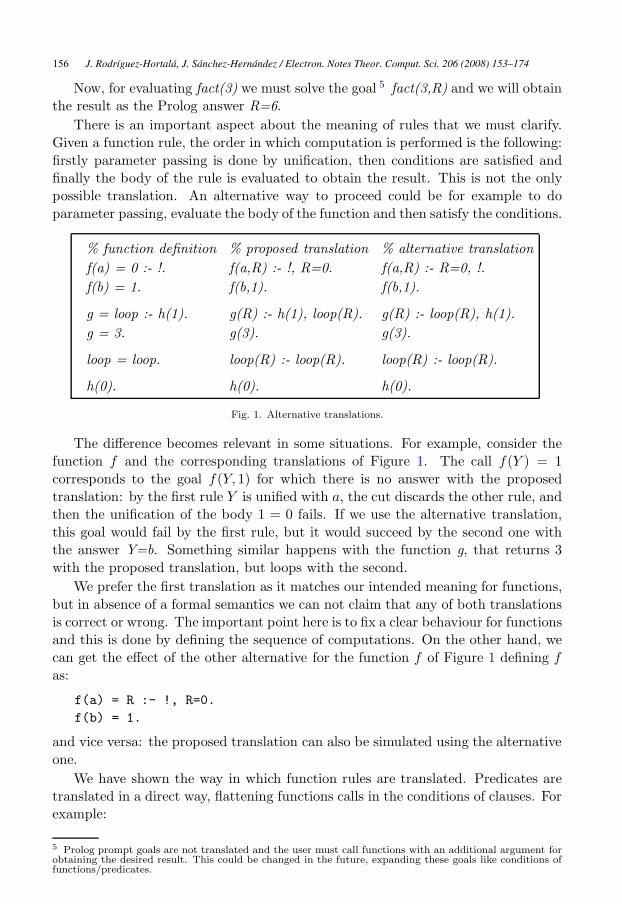
There is an important aspect about the meaning of rules that we must clarify.

Given a function rule, the order in which computation is performed is the following:

firstly parameter passing is done by unification, then conditions are satisfied and

finally the body of the rule is evaluated to obtain the result. This is not the only

possible translation. An alternative way to proceed could be for example to do

parameter passing, evaluate the body of the function and then satisfy the conditions.

% function definition

f(a) = 0 :- !.

f(b) = 1.

g = loop :- h(1).

g = 3.

loop = loop.

h(0).

% proposed translation

f(a,R) :- !, R=0.

f(b,1).

g(R) :- h(1), loop(R).

g(3).

loop(R) :- loop(R).

h(0).

% alternative translation

f(a,R) :- R=0, !.

f(b,1).

g(R) :- loop(R), h(1).

g(3).

loop(R) :- loop(R).

h(0).

Fig. 1. Alternative translations.

The difference becomes relevant in some situations. For example, consider the

function f and the corresponding translations of Figure 1. The call f(Y ) = 1

corresponds to the goal f(Y, 1) for which there is no answer with the proposed

translation: by the first rule Y is unified with a, the cut discards the other rule, and

then the unification of the body 1 = 0 fails. If we use the alternative translation,

this goal would fail by the first rule, but it would succeed by the second one with

the answer Y=b. Something similar happens with the function g, that returns 3

with the proposed translation, but loops with the second.

We prefer the first translation as it matches our intended meaning for functions,

but in absence of a formal semantics we can not claim that any of both translations

is correct or wrong. The important point here is to fix a clear behaviour for functions

and this is done by defining the sequence of computations. On the other hand, we

can get the effect of the other alternative for the function f of Figure 1 defining f

as:

f(a) = R :- !, R=0.

f(b) = 1.

and vice versa: the proposed translation can also be simulated using the alternative

one.

We have shown the way in which function rules are translated. Predicates are

translated in a direct way, flattening functions calls in the conditions of clauses. For

example:

5 Prolog prompt goals are not translated and the user must call functions with an additional argument forobtaining the desired result. This could be changed in the future, expanding these goals like conditions offunctions/predicates.


doubleFact(N,M) :- fact(N)=F, M=2*F.

is translated into:

doubleFact(N,M):- fact(N,F1), F1=F, *(2,F,M1), M=M1.

Another interesting thing when mixing functions and predicates may be to use

a predicate as a function choosing one or some arguments of the predicate as the

returning value(s) of the function. The file prelude provides a projection function

proj for this purpose. This projection is useful in general to exploit the built-in

predicates of Prolog in a functional style. A call of the form proj(T,G) evaluates

the goal G and returns the Prolog term T with the corresponding bindings for

variables. For example, the following function takes a Prolog term and returns a

pair with the main functor and the arity of it:

fun_ar(Term) = proj((Name,Arity), functor(Term,Name,Arity)).

The call fun ar(a(b,X)) returns the pair (a,2).

3 Higher order functions and λ-abstractions

For higher order functions we perform a translation into first order using a well

known technique that was also implemented in the language Toy [4]. The idea is

to consider every partial application as a Prolog term instead of a proper function

call and to use a new function @ (read apply) for applying these partial applications

to arguments. The function @ is defined as an infix operator and the translation

generates its rules for (every partial application of) all the functions of the program.

As an example, consider the program:

map(F,[]) = [].

map(F,[X|Xs]) = [F@X|map(F,Xs)].

neg(L) = map(not,L).

not(true) = false.

not(false) = true.

Notice the explicit use of the function @ in the second rule. The translation pro-

duces:

map(F,[],R) :- R=[].

map(F,[X|Xs],R) :- @(F,X,Fx), ap(F,Xs,Fxs), R=[Fx|Fxs].

neg(L,R) :- map(not,L,L1), R=L1.

not(true,R) :- R=false.

not(false,R) :- R=true.

together with the rules for @ corresponding to partial applications of all the func-

tions of the program:


neg([true,false,false],L) � (neg)

map(not,[true,false,false],L1), L=L1 � (map2)

@(not,true,Fx), map(not,[false,false],Fxs), L1=[Fx|Fxs], L=L1 � (@4)

not(true,Fx), map(not,[false,false],Fxs), L1=[Fx|Fxs], L=L1 � (not1)

Fx=false, map(not,[false,false],Fxs), L1=[Fx|Fxs], L=L1 � (=)

map(not,[false,false],Fxs), L1=[false|Fxs], L=L1 � (map1)

. . .

L=[false,true,true]

Fig. 2. Higher order goal example

@(map,F,map(F)).

@(map(F),L,L1) :- map(F,L,L1).

@(neg,L,L1) :- neg(L,L1).

@(not,X,Y) :- not(X,Y).

Figure 2 shows the resolution steps for evaluating neg([true,false,false]), i.e., the

goal neg([true,false,false],L) using this translation. The clause used in each step is

annotated on the right. The step marked with (@4) evaluates the partial application

not on the argument true, obtaining the (total) application not(true,Fx). And the

next step (marked with (not1)) evaluates this call obtaining Fx=false. The rest of

steps proceed in a similar way until getting the expected answer L=[false,true,true].

The system also allows λ-abstractions or anonymous functions of the form

λx.e using the syntax fun(x,e). In general, a generalized abstraction of the form

λx1 . . . xn . e can be written as:

fun(x1, . . . , xn︸︷︷︸arguments

, e︸︷︷︸body

)

In a first step, the translation introduces a new function funN for each anonymous

function (where N is a counter of λ-abstractions of the program). The function

funN is defined according to the arguments and body of the λ-abstraction and the

abstraction itself is replaced by a call to funN. For example, the function:

f(L) = map(fun(X,X*2),L).

will be translated in this first step to:

f(L)=map(fun1,L).

fun1(X)=X*2.

In a second step these functions are translated in the usual way. Notice that in

general the body of a λ-abstraction can use variables that are not arguments of the

abstraction itself, but come from the external context. For example, we can define:

g(X) = fun(Y,X+Y).


Here X is not an argument of the abstraction but it appears in the body. Every

argument of this kind must be passed to the function funN, so the first step would

produce in this case:

g(X) = fun2(X).

fun2(X,Y) = X+Y.

Here fun2(X) is a partial application that expects an argument Y for evaluating.

The system checks the arities of the functions and generates the appropriate apply’s

for them.

4 Lazy evaluation in strict languages

The question about laziness versus strictness is an old debate in the functional

community. From a theoretical point of view, lazy evaluation may be preferred to

eager evaluation, but from a practical point of view both alternatives have good

arguments to support them. A detailed discussion on this topic is beyond the aim

of this paper, but we can point out that eager evaluation is usually considered to be

more efficient than lazy evaluation in general, while lazy evaluation is a very nice

resource for the programmer to encode elegant solutions for problems that involve

infinite (or incomplete) data structures.

We adopt a middle way: our functions are strict by default, but we allow lazy

evaluation by means of explicit annotations. This idea is not new as the functional

extension of Prolog proposed in [5] allows lazy annotations for functions. Further-

more, some strict functional languages such as OCaml provide resources to suspend

the evaluation of expressions and to force its evaluation when needed. In the next

Sections we explore these approaches.

4.1 Lazy annotations on functions

The proposal of [5] allows to declare a function to be evaluated lazily. In the

translation to Prolog predicates, the evaluation of those functions is suspended until

the result is demanded by unification at some predicate. This is done by means of

the primitive control freeze(Var,Goal) that delays the execution of Goal until Var

is bound. To illustrate this translation consider the following program:

from(N) = [N|from(N+1)].

take(0,L) = [] :- !.

take(N,[]) = [] :- !.

take(N,[X|Xs]) = [X|take(N-1,Xs)].

firstNats(M) = take(M,from(1)).

If these functions are translated as explained before it is easy to understand that the

evaluation of the function firstNats(3) will not terminate due to the non-termination

of from. But declaring the function from to be lazy allows to make a different


translation for it (the translation for take and firstNats does not change):

from(N,L):- freeze(L,fromLazy(N,L)).

fromLazy(N,[N|L]):- +(N,1,N1), from(N1,L).

Now consider again the evaluation of the function firstNats(3), i.e., the

goal firstNats(3,L). The goal from(1,L1) generates a suspended call to from-

Lazy(1,L1). The variable L1 will be demanded by unification when evaluating

take(3,L1,L). Then we obtain a list with head 1 followed by a suspended call to

fromLazy(2,L2). In this way we obtain a list with the elements 1,2 and 3, followed

by a suspended call to take(0, <susp>, K) that provides the answer K = [] using

the first clause of take.

The translation is simple and works as expected, but it is difficult in general to

select the set of functions that must be declared as lazy in a program. A non appro-

priate selection can produce non-termination or an inefficient translation. Consider

the classic sieve of Eratosthenes for generating the (infinite) list of primes, pro-

grammed as follows:

primes = sieve(from(2)).

sieve([X|Xs]) = [X | sieve(filter(fun(Y,mod(Y,X)=\=0), Xs))].

firstPrimes(N) = take(N,primes).

The functions from and take are defined as in the previous example. The function

filter(P,L) removes from the list L those elements that do not satisfy the property

P (P must be a boolean function). Then filter(fun(Y,mod(Y,X)=\=0),Xs) removes

the multiples of X from Xs. Finally, firstPrimes(N) returns the first N prime num-

bers.

If we make no lazy declaration, every call to fistPrimes will loop because from

produces an infinite list, so we should declare from as a lazy function. But the

program still loops, because filter will demand the evaluation of the (complete)

list. Then we should also declare filter as a lazy function. The program still loops

because sieve recursively requires the evaluation of the list. A solution could be to

make lazy annotations for every function in the program, thus getting a completely

lazy program. This works, but the program would be quite inefficient. In fact, for

this particular case, the program will work just declaring the functions from, filter

and sieve to be lazily evaluated. This short example shows that it is not easy to

locate the appropriate functions that must be lazily evaluated, and the problem

would become very hard with large programs.

Notice that in the previous examples what is actually needed to be lazy are lists

as a data type, more than a concrete set of functions of the program. This idea will

guide the treatment of laziness that we propose.


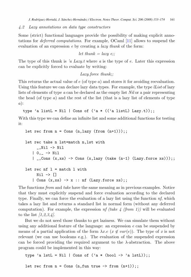
4.2 Lazy annotations on data type constructors

Some (strict) functional languages provide the possibility of making explicit anno-

tations for deferred computations. For example, OCaml [11] allows to suspend the

evaluation of an expression e by creating a lazy thunk of the form:

let thunk = lazy e;;

The type of this thunk is ’a Lazy.t where a is the type of e. Later this expression

can be explicitly forced to evaluate by writing:

Lazy.force thunk;;

This returns the actual value of e (of type a) and stores it for avoiding reevaluation.

Using this feature we can declare lazy data types. For example, the type lList of lazy

lists of elements of type a can be declared as the empty list Nil or a pair representing

the head (of type a) and the rest of the list (that is a lazy list of elements of type

a):

type ’a listL = Nil | Cons of (’a * ((’a listL) Lazy.t));;

With this type we can define an infinite list and some additional functions for testing

it:

let rec from n = Cons (n,lazy (from (n+1)));;

let rec take n lst=match n,lst with

_,Nil -> Nil

| 0,_ -> Nil

| _,Cons (x,xs) -> Cons (x,lazy (take (n-1) (Lazy.force xs)));;

let rec nf l = match l with

Nil -> []

| Cons (x,xs) -> x :: nf (Lazy.force xs);;

The functions from and take have the same meaning as in previous examples. Notice

that they must explicitly suspend and force evaluation according to the declared

type. Finally, we can force the evaluation of a lazy list using the function nf, which

takes a lazy list and returns a standard list in normal form (without any deferred

computation). For example, the expression nf (take 4 (from 1)) will be evaluated

to the list [1,2,3,4].

But we do not need those thunks to get laziness. We can simulate them without

using any additional feature of the language: an expression e can be suspended by

means of a partial application of the form λx.e (x �∈ var(e)). The type of x is not

relevant (we can use booleans e.g.). The evaluation of the suspended expression

can be forced providing the required argument to the λ-abstraction. The above

program could be implemented in this way:

type ’a lstL = Nil | Cons of (’a * (bool -> ’a lstL));;

let rec from n = Cons (n,fun true -> from (n+1));;


let rec take n lst=match n,lst with

_,Nil -> Nil

| 0,_ -> Nil

| _,Cons (x,susp) -> Cons (x, fun true

-> take (n-1) (susp true));;

let rec nf l = match l with

Nil -> []

| Cons (x,susp) -> x :: nf (susp true);;

This last version contains essentially the idea that we will incorporate to our trans-

lation, but it presents a problem: while the first version implicitly provides sharing

(because OCaml stores the computed result after the evaluation of a thunk, for

avoiding reevaluation), the second one does not. In our context this is not only a

problem of efficiency, but the intended semantics could be destroyed as we will see

in Section 5.2.

5 Our approach to laziness

In our setting we provide laziness annotations for data type constructors. With only

this information, the translator will introduce the appropriate suspensions and the

corresponding manipulation for them. We start showing a basic translation scheme

and then an extension to capture sharing.

5.1 A first translation schema

Consider for example, the program for from of Section 4.1, that now can be easily

encoded as:

:- lazy([_|on]).

from(N) = [N|from(N+1)].

take(0,L) = [] :- !.

take(N,[]) = [] :- !.

take(N,[X|Xs]) = [X|take(N-1,Xs)].


The first line declares the Prolog constructor for lists [ | ] to be lazy in the second

argument (similar to what is done in the OCaml version). In a preprocessing step,

at the level of functional definitions, the translator replaces the (declared) lazy

arguments of constructors by λ-abstractions:

from(N,L) = [N|fun(_,from(N+1))].


take(0,L) = [] :- !.

take(N,[]) = [] :- !.

take(N,[X|Xs]) = [X|fun(_,take(N-1,Xs@dummy))].


The rest of the list in the body of from has been replaced by the λ-abstraction

fun( ,from(N+1)). This abstraction takes a (dummy) anonymous variable as argu-

ment and returns the original expression from(N+1). The last rule of take contains

also a λ-abstraction, but here the situation is a little more complex. The variable

Xs comes from the second argument of a list in the head, so it is a suspended expres-

sion. In order to pass it to take in the body first we need to wake it up. This is done

by applying a dummy argument to it (the constant dummy could be replaced by

any other term). The general criteria for manipulating suspensions is to introduce

them as arguments of constructor symbols that have been declared as lazy (in our

example, any tail of a list), and to wake them up when they are used as arguments

of functions or constructors that have no such arguments declared as lazy. On the

other hand, any variable argument in a constructor, at a position declared as lazy

must represent a suspension at run time (in the last rule of take, the variable Xs

is in this situation and it must be woken up when used as an argument for take in

the body). Notice that although we are not considering types in our functions, the

suspensions obey a discipline of types (as it was the case with the OCaml version).

The next step of the translation will produce the clauses for these rules as

explained in Sections 2 and 3, with the corresponding clauses for λ-abstractions

and partial applications. With this translation we could now evaluate the goal

firstNats(6,L). The resulting answer could be a little surprising:

L = [1|fun2(...)]

This is correct, as the second argument of lists is a suspended form. In the OCaml

version something similar happened and we had to implement a function nf to obtain

a normal form (a completely evaluated expression). Our translator incorporates a

predefined predicate nf with the same purpose, so we could throw the goal first-

Nats(6,L1), nf(L1,L) and obtain the expected answer 6 : L = [1,2,3,4,5,6]. This

scheme works fine, except that it does not consider any sharing, and this can be

catastrophic as we will see in the next section.

5.2 Call-time choice and sharing

The previous translation can have an undesirable (or at least unexpected) behaviour

when non-determinism is involved. Let us examine an example to illustrate the

situation. Consider the classical Prolog generate and test algorithm for sorting

a list: generate permutations of the list in a non-deterministic way and test if

they are sorted. This algorithm, using (non-deterministic) functions can be easily

implemented in Functional Prolog as:

6 The predicate nf could be implicitly called in future versions of the translator.


permut([]) = [].

permut([X|Xs]) = insert(X,permut(Xs)).

insert(X,[]) = [X].

insert(X,[Y|Ys]) = [X,Y|Ys].

insert(X,[Y|Ys]) = [Y|insert(X,Ys)].

sorted([]) = true.

sorted([X]) = true.

sorted([X,Y|Ys]) = sorted([Y|Ys]) :- X=<Y.

sorted([X,Y|Ys]) = false :- X>Y.

permutSort(Xs) = ifThen(sorted(Ys),Ys) :- Ys=permut(Xs).

The function permut returns a permutation of the list by inserting the head of

such a list into a permutation of the rest of the list; insert puts an element into a

list at any possible possition (by backtraking). The function sorted checks if the

given list is sorted. And finally, permutSort generates a permutation of the list

and if it is sorted then returns it (if it is not sorted, by backtraking will search for

another permutation). The function sorted checks if the given list is sorted. And

finally, permutSort generates permutations of the list searching for a sorted one

by backtracking. The function ifThen is defined in the prelude with the standard

meaning.

This algorithm works fine, except for the efficiency. The worst case corresponds

to a list in reverse order. For example, the goal permutSort([4,3,2,1],L) will produce

all the possible permutations of the list before finding the sorted one. This example

has become also a classical one in Toy and Curry. Moreover it works much better

in Toy and Curry because of laziness. Prolog’s and the eager version above must

generate permutations completely and then make the test, but with lazy evaluation

permutations can be discarded without being fully generated. For example, for

sorting the list [4,3,2,1] an eager version will generate all the permutations of the

form [3,1,. . . ] while the lazy version can discard all of them as the first two elements

(3,1) are not sorted (see [12] for a detailed analysis of this algorithm).

Here, there is not any infinite data structure involved, but laziness is inter-

esting for the sake of efficiency. Then we can use lazy lists with the declara-

tion :- lazy([_|on])., but then a new problem appears. The goal permut-

Sort([4,3,2,1],L) will produce six “ordered” lists:

[1, 4, 3, 2] [1, 3, 4, 2]. . . [1, 2, 3, 4]

that correspond to the element 1 followed by any permutation of [2,3,4]. The

problem comes from the two occurrences of the variable Ys in the rule

permutSort(Xs) = ifThen(sorted(Ys),Ys) :- Ys=permut(Xs).

As we are using lazy lists, the condition Ys=permut(Xs) produces partially

evaluated permutations of [4,3,2,1] of the form [elem|λ .permut(rest)], where


elem is an element of [4,3,2,1] and rest contains the remaining elements. In

particular, by backtracking we will find the (partially evaluated permutation)

Ys=[1|λ .permut([4,3,2])]. This variable Ys is used as an argument in the body

of permutSort and then the abstraction is duplicated:

ifThen(sorted([1|λ .permut([4,3,2])]), [1|λ .permut([4,3,2])])

This corresponds to a run-time choice semantics as both calls can evolve indepen-

dently. The evaluation of sorted([1|λ .permut([4,3,2])]) can be evaluated to true

as permut[4,3,2] can produce (by backtracking) the list [2,3,4]. Then permutSort

returns the list [1|λ .permut([4,3,2])], that by normalization can produce the six

answers mentioned before.

How can we solve this problem? Or equivalently: how can we implement shar-

ing? The solution uses a technique similar to one implemented in Toy [4] for similar

purposes. In our case, it can be implemented extending the λ-abstractions intro-

duced for suspensions with two more arguments (Prolog variables): a flag Ev for

indicating if the suspension has been evaluated before or not, and the result Res of

such an evaluation in affirmative case. The new δ-abstractions have the form:

δ Ev Res . expr

The dummy argument has the same meaning as before, Ev can be the term on or

a variable and Res can be any Prolog term. The application of a δ-abstraction to

the dummy argument is defined as:

@(δ Ev Res . expr, dummy)=

⎧⎨⎩

Res if Ev==on

expr otherwise

This idea can be easily implemented in Prolog. δ-abstractions are represented

by Prolog terms of the form funN(Ev,Res, ,<Expr>) (N is a counter for getting

different names for the abstractions). These abstractions are flattened as explained

in Section 3, but their rules must consider the parameters used for sharing:

funN(Ev,Res,ExprRes) = H :- (Ev==on, ! ; ExprRes , Ev=on), H=Res.

This rule first checks if the expression has been previously evaluated by looking up

the flag Ev. In such a case, the resulting value is the one stored in Res. In other

case we evaluate Expr, set the flag and return the obtained value. The notation

ExpRes indicates that the expression Exp must be flattened in such a way that the

resulting value is Res. For example, the function app is defined in the prelude as:

app([], Xs) = Xs.

app([X|Xs], Ys) = [X|app(Xs, Ys)].

and it is translated as:

app([],Ys,Ys).

app([X|Xs],Ys,[X|fun1(Ev, Res, Xs, Ys)]).

fun1(Ev,Res,Xs,Ys,Dummy,H):-

(Ev==on, !


Goal Eager Lazy funs (all) Lazy funs (some) Lazy lists

nPrime(300) - 0.829399 0.534276 0.182028

nPrime(600) - 2.65868 1.70961 0.697245

nPrime(1000) - overflow overflow 1.92277

nPrime(6000) - overflow overflow 80.5051

firstPrimes(300) - 1.06425 0.543337 0.230733

firstPrimes(600) - 3.58354 1.76382 0.899285

firstPrimes(1000) - overflow overflow 2.19576

firstPrimes(1200) - overflow overflow 3.39396

firstPrimes(1500) - overflow overflow overflow

permutSort(revLst(10)) 8.75339 0.365988 0.160308 0.195278

permutSort(revLst(12)) 1000.51 3.18058 1.44293 1.70397

permutSort(revLst(15)) . . . 96.7763 42.2988 49.6788

permutSort(revLst(16)) . . . 248.329 110.585 128.547

Fig. 3. Lazy functions versus lazy constructors (times in seconds)

;

@(Xs, dummy, XsEv), app(XsEv, Ys, R1), H=R1, Ev=on),

H=Res.

Now, coming back to our example, the function permutSort works as desired and

the goal permutSort([4,3,2,1],L) will produce a unique answer L=[1,2,3,4]. Using

lazy lists the algorithm is drastically improved in efficiency as expected. Moreover,

the translation incorporates some (quite technical) optimizations that improve the

efficiency even more.

6 Examples and performance

In this section we will give an idea of the capabilities of the functional Prolog model

proposed in this work and its performance. We are interested in the comparison

with similar approaches, in particular, with functional-logic programming and with

the approach of [5] that we have summarized in Section 4.1.

The next interesting comparison may be with respect to functional-logic sys-

tems, as they also use non-deterministic functions and laziness. Moreover, some

implementations as Toy [4] and Packs [10] make a translation into Prolog, what

justifies even more the comparison.

It is more difficult to compare our translation with functional languages such

as Haskell or OCaml because those programming styles are very different from

our proposal, mainly because they are deterministic languages. We have made

some tests using examples in which non-deterministic functions are not used, and

both Haskell’s and OCaml’s versions had an improved performance compared with

functional Prolog.

All the tests have been done under an Intel Pentium 4 EM64T 3.20 GHz with 1

Gb of RAM memory.


6.1 Lazy functions and lazy constructors

The approach of laziness of Section 4.1 was introduced in [5] as an extension to

Ciao Prolog [3]. That proposal is very close to our current approach, as both are

functional extensions of Prolog, with optional laziness. It is different from ours

in its treatment of higher order and some other aspects, but the most interesting

difference is with respect to laziness. Unfortunately, the implementation is not

included in the Ciao Prolog distribution and so we must use the translation scheme

seen in Section 4.1 for comparison.

As we have pointed out in Section 4.1, implementing this model for laziness is

quite straightforward just using the resources of standard Prolog for delaying com-

putations. This approach has the advantage that most of the work about laziness

is automatically done by Prolog, using its capabilities for delaying goals. Never-

theless, this model of laziness can be hard to manipulate as, in general, choosing

which program functions must be lazily evaluated is not a trivial issue. As an easy

solution we could turn every function lazy, but in this case the efficiency of the

program would be seriously affected.

Figure 3 shows some experimental measurements using the sieve of Eratosthenes

of Section 4.1 and the permutation sort algorithm of Section 5.2 (revLst(N) returns

a list of length N in reverse order, which is the worst case for this algorithm). The

first column contains the goals to solve, the second shows the time measurements

for the program without any lazy declaration (nPrimes and firstPrimes do not

terminate), and columns Lazy funs (all and some) contain the running times for

the translation of Section 4.1, declaring all functions as lazy and only some of them

as lazy, respectively. For the sieve, the colum some has been obtained declaring

lazy only from, filter and sieve (the minimal laziness needed to ensure termination

for the corresponding goal), and for the sorting algorithm only insert is declared

as lazy. The last column corresponds to the proposed translation, with lazy lists

declared in the program as :- lazy([_|on]). The experiments show that using

lazy functions, an appropriate selection of the lazy ones is important to achieve a

more efficient program. Using lazy constructors we must not worry about which

functions must be declared as lazy, and this version is more efficient in time and

space for the sieve. In the case of sorting, the performance of the version with some

lazy functions is similar to the one for lazy constructors.

Functional-logic languages like Toy and Curry are also close to the proposal of

this paper, as they use lazy non-deterministic functions and logic variables. Further-

more, these languages are usually implemented by a compilation into Prolog code.

We have tested the permutSort algorithm presented in Section 5.2 in our functional

Prolog translation and Toy (with minor syntactic changes). Figure 4 shows that

the performance is improved significantly in the functional Prolog version.

The second example of Figure 4 is more interesting as the differences come

directly from the lazy models that we are using. The function fib(N) evaluates

the N-nth number of the Fibonacci series. It is implemented with exponential

complexity (fib(0)=0; fib(1)=1; fib(N)=fib(N-1)+fib(N-2)). A goal like


Input list Toy Lazy lists

revLst(10) 0.76 0.28

revLst(12) 6.90 2.35

revLst(12) 6.90 2.35

revLst(12) 62.43 22.97

[fib(22),fib(21),fib(20)] 1.16 1.13

[fib(26),fib(25),fib(24)] overflow 7.65

Fig. 4. Toy and functional Prolog with lazy lists. Goal: permutSort(<list>) (times in seconds)

permutSort([fib(22),fib(21),fib(20)])

has an undesired behaviour in Toy as it needs to reevaluate each item of the list

several times, as the value is not reused when trying another permutation for sorting

the list. This is not the case with our model of laziness, as only lists are lazily

evaluated. The calls to fib are evaluated only once and then the sorting algorithm

proceeds to sort the list.

6.2 Mixing lazy and eager evaluation

Having lazy annotations for constructors allows to get a finer control on the evalu-

ation and achieve a better performance in some situations. We illustrate this topic

with Pascal’s triangle in the next example. Such a triangle is an infinite structure

of the form:

1 row 0

1 1 row 1

1 2 1 row 2

1 3 3 1 row 3

1 4 6 4 1 row 4

. . .

Each row can be represented as a list, hence being the triangle an infinite list

of lists. In general, the row i-nth (i > 0) is obtained adding pair of consecutive

elements of the previous row and putting 1 as the first and last element in the

resulting row. Given a row F , say [1, 3, 3, 1] we can elegantly obtain the next row as

follows: we build the lists [0, 1, 3, 3, 1] and [1, 3, 3, 1, 0] and then add the elements at

the same positions obtaining the list [1, 4, 6, 4, 1]. This process can be done within

a single (functional) expression:

zipWith((+),[0|F],app(F,[0])).

The function zipWith is defined as:

zipWith(F,[],Xs) = [] :-!.

zipWith(F,Xs,[]) = [] :-!.

zipWith(F,[X|Xs],[Y|Ys]) = [(F@X)@Y|zipWith(F,Xs,Ys)].

and app stands for the concatenation of lists.


With these ideas, a function pas for evaluating the triangle of Pascal can be

written as:

:-include(prelude).

:- lazy([_|on]).

iter(F) = [F|iter(zipWith((+),[0|F],app(F,[0])))].

pas = iter([1]).

% testing functions

row(N) = nth(N,pas).

comb(N,M) = nth(M,(nth(N,pas))).

The function iter(F) evaluates all the next rows (an infinite number) from a given

row F and pas calls it with the initial row [1] to obtain the complete triangle. The

functions row and comb are functions for testing the program (nth(N) is defined in

the prelude and returns the N-nth element of a list, starting at position 0). row(N)

returns the N-th row of the triangle and comb(N,M) returns the combinatorial

number(

NM

)using the fact that the M-nth element of the N-nth row of the triangle

is exactly that combinatorial number. We can obtain for example the row 8 of the

triangle by throwing the goal row(8,K), nf(K,L):

L = [1, 8, 28, 56, 70, 56, 28, 8, 1]

or we can obtain the combinatorial number(18

5

)with comb(18,5,N) getting N=8568.

Notice that due to the lazy evaluation of lists, the first goal only evaluates the

first 8 rows, and the second one evaluates only the initial prefix of the first 18 rows

(for example it does not need to evaluate(1614

)).

Goal All lazy Lazy/eager

row(400) 0.691386 0.248232

row(600) 1.77859 0.560645

row(800) overflow 1.01706



comb(500, 250) 0.87144 0.561656

comb(800, 400) 2.13438 2.18744

comb(1000, 500) 5.29124 4.3969

Fig. 5. Mixing lazy and eager evaluation

Having laziness associated to data type constructors instead of functions provides

a finer control over the construction of data structures. In this example, we use

(lazy) lists both for representing the rows of the triangle and also to collect those

rows, but one could think about these lists as different kinds of structures. In

particular, if we were interested in getting complete rows of the triangle (first goal

above),we could improve this code by distinguishing two data type structures. Rows

could be represented as (a new kind of) lists with constructors nil and cons:

row ::= nil | cons(e,row)


These rows would be strictly evaluated, and we could use lazy lists as we did before

for collecting the rows of the triangle as follows:

:- include(prelude).

:- lazy([_|on]).

iter2(F) = [F|iter2(zipWithRows((+),cons(0,F),

appendRows(F,cons(0,nil))))].

pas2 = iter2(cons(1,nil)).

row2(N) = nth(N,pas2).

where zipWithRows and appendRows are the versions for zipWith and app, but for

the rows we are using. This program is faster than the previous one, specially for

getting an entire row of the triangle (see Figure 5).

6.3 Metaprogramming

In practice, it is very usual to use meta-predicates when programming in Prolog.

In this section we show how our functional extension can be useful combined with

meta-programming. We explore the classic count-down problem: we must find how

to combine a list of operands (integers) by means of arithmetical operations to

obtain a given total. This problem can be solved by a generate-and-test algorithm:

generate a expression in a non-deterministic way and test if it is a solution, i.e., if

its evaluation gives the required total.

Figure 6 shows the program for solving this problem. An expression can be

either a number or an operator applied to two expressions. We use several (non-

deterministic) functions for generating expressions: oneOf(L) returns an element of

the list L; split(L) divides the list L into two sublists; and genExp(Ns) uses these

functions to build an expression with the numbers of Ns.

The term decomposition predicate =.. combined with the function oneOf allows

for an elegant definition of genExp(Ns).

The evaluation function eval is defined in a natural way using Prolog cuts (the

last rule stands for a single number). The rule for division must make some tests

as it is understood as integer division. Finally, the function sol(V,L) generates

an expression with the operands of the list L and tests if it is a solution. By

backtracking this function will find the solution for the problem if it exists. For

example, sol(28,[3,6,4,5]) will return mult(plus(5, div(6, 3)), 4), that is, (5+6/3)*4.

If we evaluate sol(26,[4,5,3]) we do not obtain any solution as the numbers 4, 5

and 3 do not allow to get the exact value 26. It would be interesting to obtain the

best approximation to the solution from the program above. A typical solution in

Prolog for this kind of problems is to use some meta-predicates to explore the search

space. Using higher order functions we can encapsulate this search operation. It

would be nice to have a function

best(Gen,Data,Comp)


% expression ::= number | plus exp exp | minus exp exp

| mult exp | div exp exp

% non deterministic generation of expressions

genExp(Ns) = oneOf(Ns).

genExp(Ns) = E :-

split(Ns)=(As,Bs),

E=..[oneOf([plus,minus,mult,div]),genExp(As),genExp(Bs)].

oneOf([N|Ns]) = N.

oneOf([N|Ns]) = oneOf(Ns).

split([X,Y]) = ([X],[Y]).

split([X,Y]) = ([Y],[X]).

split([N|Ns]) = S :- split(Ns)=(As,Bs),

(S=([N|As],Bs); S=(As,[N|Bs])).

% evaluation of expressions

eval(plus(E1,E2)) = eval(E1)+eval(E2) :- !.

eval(minus(E1,E2)) = eval(E1)-eval(E2) :- !.

eval(mult(E1,E2)) = eval(E1)*eval(E2) :- !.

eval(div(E1,E2)) = V1/V2 :-

!, V1=eval(E1), V2=eval(E2),

V2\==0, V1>V2, mod(V1,V2)==0.

eval(N)=N.

% solution for the count-down problem

sol(V,L)=E :- E=genExp(L), V==eval(E).

Fig. 6. Arithmetical expressions: generation and evaluation

that returns the best alternative given: a non-determistic function Gen that gener-

ates the search space using the arguments provided in Data, where the best solution

depends on a comparison criteria Comp. This function would allow to get the best

approximation to a value V given a list of numbers L as:

bestApprox(V,L) = best(genExpVal,[V,L],better).

genExpVal(V,L) = (E,abs(V-eval(E))) :- genExp(L)=E.

better((E1,V1),(E2,V2)) = (E1,V1) :- V1<V2, !.

better((E1,V1),(E2,V2)) = (E2,V2).

Here the function genExpVal(V,L) returns a candidate to solution: a pair with an

expression built-up with the numbers of L and the valorization (not evaluation) of

that expression according to the problem. In this problem the valorization is the

difference between the value we are searching for V and the result of evaluating the


expression. For example, genExpVal(17,[3,4,1]) may return (3*4+1,4) as 3*4+1=13

and the difference with the total 17-13=4; another result may be (3*4,5) as 17-

12=5. The function better(C1,C2) returns the best between the candidates C1 and

C2, where a candidate is a pair expression-valorization as we have seen. Now, for

the expression bestApprox(26,[4,5,3]) we would obtain the expression mult(3, plus(5,

4)) and the valorization 1 (3*(5+4)=27 and 27-26=1).

The only open question is how to define the function best(Gen,Data,Comp). Fig-

ure 7 shows the code for this function. It initiates the search producing a candidate

and asserting it as the best solution for the moment. Then, bestAux generates all

the possible candidates updating the best solution found at each step.

The important fact is that this function best can be used to solve a variety of

problems of optimization. Other functions for exploring the search space can be

appropriately parametrized and encoded, analogously to the encapsulated search

primitives of Curry [2].

best(F,Args,Better) = R :-

applyLst(F,Args)=EV, retractall(currentBest(_)),

assert(currentBest(EV)), !, bestAux(F,Args,Better)=R.

bestAux(F,Args,Better)= R :-

applyLst(F,Args)=E, currentBest(C),

applyLst(Better,[E,C])=E, retractall(currentBest(_)),

assert(currentBest(E)), fail.

bestAux(_,_,_) = R :- !, currentBest(R).

applyLst(F,[]) = F.

applyLst(F,[X|Xs]) = applyLst(F@X,Xs).

Fig. 7. Encapsulated search for the best candidate

7 Conclusions and future work

In this work we show how to extend Prolog with functions performing a translation

of function rules into Prolog predicates. We introduce a simple syntax for func-

tion definition and a transformation of higher order to first order syntax including

lambda abstractions. With these features we can talk about functional Prolog. The

extended language implements an eager evaluation mechanism, but we explore some

alternatives for introducing lazy evaluation by means of user annotations.

It is possible to manipulate optional laziness by introducing annotations on func-

tions or on constructors. In practice it is easier to use the second alternative because

to decide which functions in a program must be lazily evaluated may be a hard task,

while it is not difficult to think about the data structures that must be lazily con-

structed. Moreover, experimental measurements show a better performance when

using lazy constructors.

The manipulation of laziness at the level of constructors can be done by in-


troducing artificial lambda abstractions that suspend the evaluation of the desired

arguments. But this approach presents two problems: for obtaining call-time choice

semantics some sharing mechanism is needed, and the explicit manipulation of lazy

constructor symbols is hard in practice and complicates the writing/reading of pro-

grams.

For the first problem we extend lambda abstractions with a sharing structure

that ensures call-time choice. For the second one, the translation incorporates a

complete mechanism for delaying computations and forcing later on their evalua-

tion. Similar transformations have been proposed for eager functional languages [6]

and are close to context-sensitive rewriting [7,14]. As a future work it would be inter-

esting to study the relation of our lazy annotations with context-sensitive rewriting,

at least for the declarative fragment of functional Prolog (excluding metaprogram-

ming).

We have presented a collection of examples showing the capabilities of the pro-

posal. In particular, we obtain a fine control on laziness that can be used to improve

the efficiency of programs. On the other hand, combining the meta-predicates pro-

vided by Prolog with the functional extension we obtain sophisticated resources for

exploring the search space.

The current translator is a Prolog file of about 500 lines of code. Some opti-

mizations and new features can be added as future work. In particular, it would be

interesting to improve the interface with the user.

Acknowledgement

We thank Paco Lopez Fraguas and the anonymous referees for their useful comments

and suggestions.

References

[1] Asvanyi, T., User’s functions in standard Prolog., in: Symposium on Programming Languages andSoftware Tools, 2003, pp. 103–114.

[2] Braßel, B., M. Hanus and F. Huch, Encapsulating non-determinism in functional logic computations,Journal of Functional and Logic Programming 2004 (2004).

[3] Bueno, F., D. Cabeza, M. Carro, M. Hermenegildo, P. Lopez and G. Puebla, “The Ciao Prolog System,Reference Manual,” The CLIP Group, School of Computer Science, Technical University of Madrid,1.10#7 edition (2006).

[4] Caballero, R. and J. Sanchez (eds.), TOY: A multiparadigm declarative language, version 2.2.3,Technical report, UCM, Madrid (2006).

[5] Casas, A., D. Cabeza and M. V. Hermenegildo, A syntactic approach to combining functional notation,lazy evaluation, and higher-order in LP systems., in: Int. Symposium on Functional and LogicProgramming, 2006, pp. 146–162.

[6] Fokkink, W., J. Kamperman and P. Walters, Lazy rewriting on eager machinery, ACM transactionson programming languages and systems 22 (2000), pp. 45–86.

[7] Giesl, J. and A. Middeldorp, Transformation techniques for context-sensitive rewrite systems, Journalof Functional Programming 14 (2004), pp. 379–427.

[8] Hanus, M., Functional logic programming: From theory to Curry, Technical report, Christian-Albrechts-Universitat Kiel (2005).


[9] Hanus (ed.), M., Curry: An integrated functional logic language (version 0.8.2), Available athttp://www.informatik.uni-kiel.de/~curry/report.html (2006).

[10] Hanus (ed.), M., “PAKCS 1.8.1, The Portland Aachen Kiel Curry System, User manual,” (2007),http://www.informatik.uni-kiel.de/∼pakcs/Manual.pdf.

[11] Leroy, X. et al., “The Objective Caml System, Version 3.10,” (2007),http://caml.inria.fr/pub/docs/manual-ocaml/index.html .

[12] Lopez-Fraguas, F., J. Rodrıguez-Hortala and J. Sanchez-Hernandez, Bundles pack tighter than lists, in:Draft Proc. of Trends in Functional Programming 2007, 2007, pp. XXIV–1–XXIV–16.

[13] Lopez-Fraguas, F. and J. Sanchez-Hernandez, T OY: A multiparadigm declarative system, in: Proc.Rewriting Techniques and Applications (RTA’99) (1999), pp. 244–247.

[14] Lucas, S., Context-sensitive computations in functional and functional logic programs, Journal ofFunctional and Logic Programming 1998 (1998).

[15] Somogyi, Z., F. Henderson and T. Conway, The execution algorithm of Mercury, an efficient purelydeclarative logic programming language, Journal of Logic Programming 29 (1996), pp. 17–64.


http://www.informatik.uni-kiel.de/~pakcs/Manual.pdf

http://caml.inria.fr/pub/docs/manual-ocaml/index.html

Documents

Functions and Lazy Evaluation in Prolog · · 2017-01-20Prolog predicates and function deﬁnitions in such a way that functions can be used ... proj for this purpose. This projection