1

Functions of multiple variables in MATLAB  MATLAB has many tools to make plots of multivariable functions. Of course, multi- mean two- in this case: we cannot visualize a function of any more variables than that.

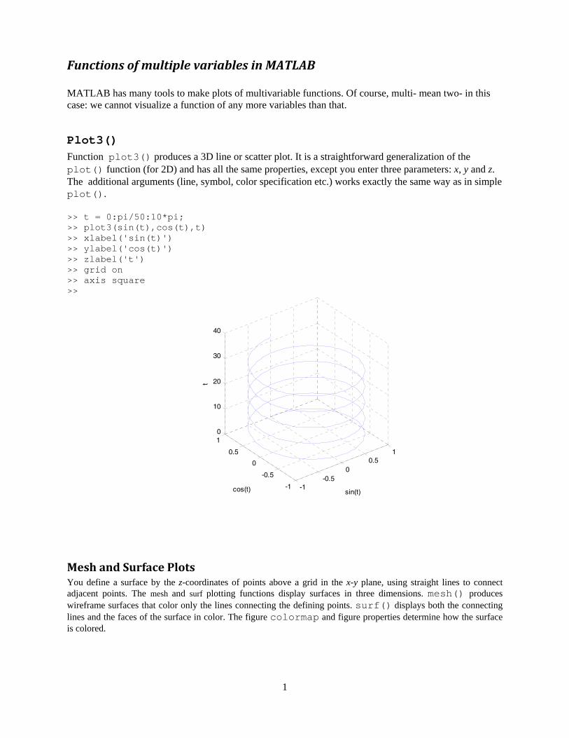
Plot3() Function plot3() produces a 3D line or scatter plot. It is a straightforward generalization of the plot() function (for 2D) and has all the same properties, except you enter three parameters: x, y and z. The additional arguments (line, symbol, color specification etc.) works exactly the same way as in simple plot(). >> t = 0:pi/50:10*pi; >> plot3(sin(t),cos(t),t) >> xlabel('sin(t)') >> ylabel('cos(t)') >> zlabel('t') >> grid on >> axis square >>

Mesh and Surface Plots You define a surface by the z-coordinates of points above a grid in the x-y plane, using straight lines to connect adjacent points. The mesh and surf plotting functions display surfaces in three dimensions. mesh() produces wireframe surfaces that color only the lines connecting the defining points. surf() displays both the connecting lines and the faces of the surface in color. The figure colormap and figure properties determine how the surface is colored.

-1-0.5

00.5

1

-1

-0.5

0

0.5

10

10

20

30

40

sin(t)cos(t)

t

2

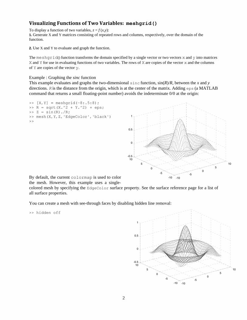
Visualizing Functions of Two Variables:  meshgrid() To display a function of two variables, z = f (x,y): 1. Generate X and Y matrices consisting of repeated rows and columns, respectively, over the domain of the function. 2. Use X and Y to evaluate and graph the function. The meshgrid() function transforms the domain specified by a single vector or two vectors x and y into matrices X and Y for use in evaluating functions of two variables. The rows of X are copies of the vector x and the columns of Y are copies of the vector y. Example : Graphing the sinc function This example evaluates and graphs the two-dimensional sinc function, sin(R)/R, between the x and y directions. R is the distance from the origin, which is at the center of the matrix. Adding eps (a MATLAB command that returns a small floating-point number) avoids the indeterminate 0/0 at the origin: >> [X,Y] = meshgrid(-8:.5:8); >> R = sqrt(X.^2 + Y.^2) + eps; >> Z = sin(R)./R; >> mesh(X,Y,Z,'EdgeColor','black') >> By default, the current colormap is used to color the mesh. However, this example uses a single-colored mesh by specifying the EdgeColor surface property. See the surface reference page for a list of all surface properties. You can create a mesh with see-through faces by disabling hidden line removal: >> hidden off

-10-5

05

10

-10

-5

0

5

10-0.5

0

0.5

1

-10-5

05

10

-10

-5

0

5

10-0.5

0

0.5

1

3

 

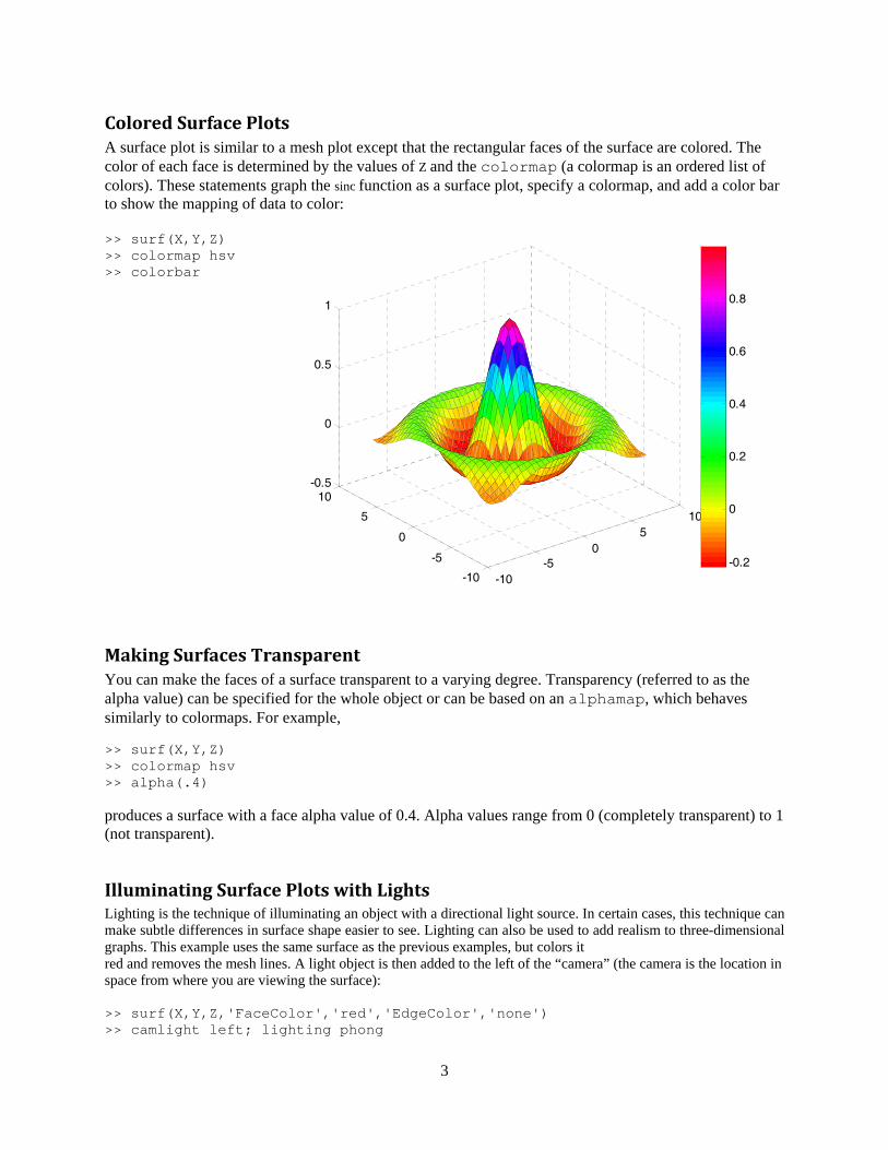
Colored Surface Plots A surface plot is similar to a mesh plot except that the rectangular faces of the surface are colored. The color of each face is determined by the values of Z and the colormap (a colormap is an ordered list of colors). These statements graph the sinc function as a surface plot, specify a colormap, and add a color bar to show the mapping of data to color: >> surf(X,Y,Z) >> colormap hsv >> colorbar

Making Surfaces Transparent You can make the faces of a surface transparent to a varying degree. Transparency (referred to as the alpha value) can be specified for the whole object or can be based on an alphamap, which behaves similarly to colormaps. For example, >> surf(X,Y,Z) >> colormap hsv >> alpha(.4) produces a surface with a face alpha value of 0.4. Alpha values range from 0 (completely transparent) to 1 (not transparent).

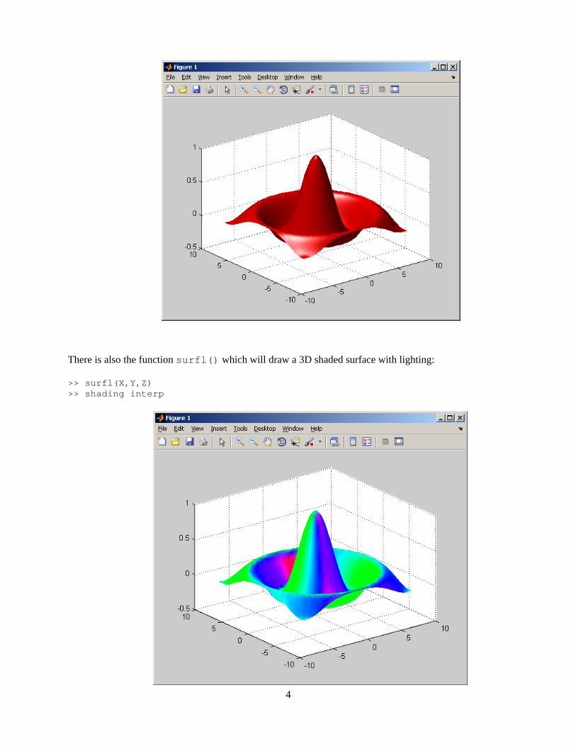
Illuminating Surface Plots with Lights Lighting is the technique of illuminating an object with a directional light source. In certain cases, this technique can make subtle differences in surface shape easier to see. Lighting can also be used to add realism to three-dimensional graphs. This example uses the same surface as the previous examples, but colors it red and removes the mesh lines. A light object is then added to the left of the “camera” (the camera is the location in space from where you are viewing the surface): >> surf(X,Y,Z,'FaceColor','red','EdgeColor','none') >> camlight left; lighting phong

-10-5

05

10

-10

-5

0

5

10-0.5

0

0.5

1

-0.2

0

0.2

0.4

0.6

0.8

4

 

 

 

 

 

 

 

 

 

 

 There is also the function surfl() which will draw a 3D shaded surface with lighting: >> surfl(X,Y,Z) >> shading interp

5

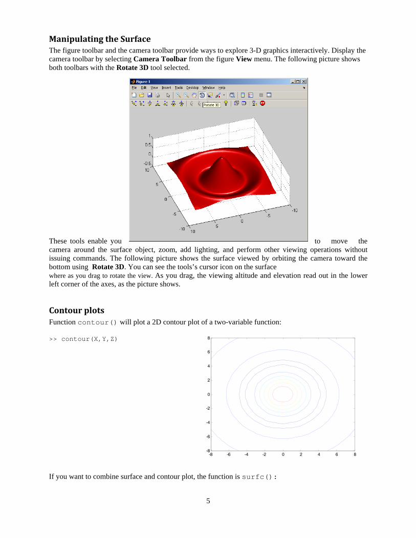
Manipulating the Surface The figure toolbar and the camera toolbar provide ways to explore 3-D graphics interactively. Display the camera toolbar by selecting Camera Toolbar from the figure View menu. The following picture shows both toolbars with the Rotate 3D tool selected. These tools enable you to move the camera around the surface object, zoom, add lighting, and perform other viewing operations without issuing commands. The following picture shows the surface viewed by orbiting the camera toward the bottom using Rotate 3D. You can see the tools’s cursor icon on the surface where as you drag to rotate the view. As you drag, the viewing altitude and elevation read out in the lower left corner of the axes, as the picture shows.

Contour plots Function contour() will plot a 2D contour plot of a two-variable function: >> contour(X,Y,Z) If you want to combine surface and contour plot, the function is surfc():

-8 -6 -4 -2 0 2 4 6 8-8

-6

-4

-2

0

2

4

6

8

6

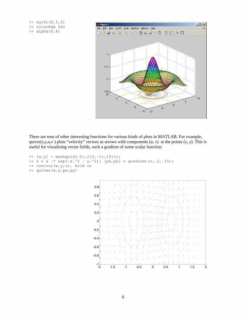
>> surfc(X,Y,Z) >> colormap hsv >> alpha(0.4) There are tons of other interesting functions for various kinds of plots in MATLAB. For example, quiver(x,y,u,v ) plots “velocity” vectors as arrows with components (u, v) at the points (x, y). This is useful for visualizing vector fields, such a gradient of some scalar function: >> [x,y] = meshgrid(-2:.2:2,-1:.15:1); >> z = x .* exp(-x.^2 - y.^2); [px,py] = gradient(z,.2,.15); >> contour(x,y,z), hold on >> quiver(x,y,px,py)

-2 -1.5 -1 -0.5 0 0.5 1 1.5 2-1

-0.8

-0.6

-0.4

-0.2

0

0.2

0.4

0.6

0.8

7

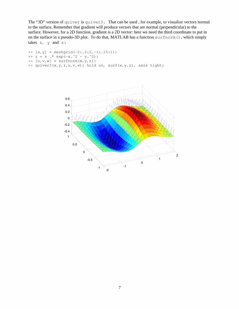
The “3D” version of quiver is quiver3. That can be used , for example, to visualize vectors normal to the surface. Remember that gradient will produce vectors that are normal (perpendicular) to the surface. However, for a 2D function, gradient is a 2D vector: here we need the third coordinate to put in on the surface in a pseudo-3D plot. To do that, MATLAB has a function surfnorm(),which simply takes z, y and z: >> [x,y] = meshgrid(-2:.2:2,-1:.15:1); >> z = x .* exp(-x.^2 - y.^2); >> [u,v,w] = surfnorm(x,y,z); >> quiver3(x,y,z,u,v,w); hold on, surf(x,y,z), axis tight;

-2-1

01

2

-1

-0.5

0

0.5

1

-0.4

-0.2

0

0.2

0.4

0.6

8

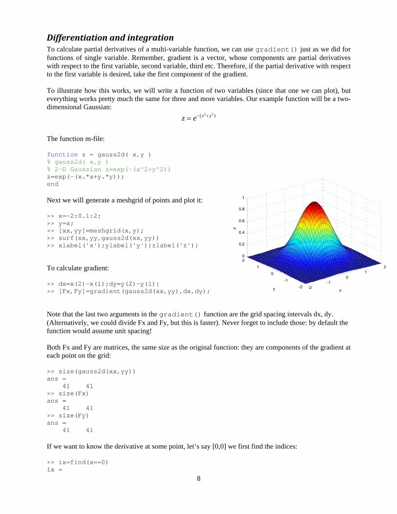
Differentiation and integration To calculate partial derivatives of a multi-variable function, we can use gradient() just as we did for functions of single variable. Remember, gradient is a vector, whose components are partial derivatives with respect to the first variable, second variable, third etc. Therefore, if the partial derivative with respect to the first variable is desired, take the first component of the gradient. To illustrate how this works, we will write a function of two variables (since that one we can plot), but everything works pretty much the same for three and more variables. Our example function will be a two-dimensional Gaussian:

)( 22 yxez

The function m-file: function z = gauss2d( x,y ) % gauss2d( x,y ) % 2-D Gaussian z=exp(-(x^2+y^2)) z=exp(-(x.*x+y.*y)); end Next we will generate a meshgrid of points and plot it: >> x=-2:0.1:2; >> y=x; >> [xx,yy]=meshgrid(x,y); >> surf(xx,yy,gauss2d(xx,yy)) >> xlabel('x');ylabel('y');zlabel('z'); To calculate gradient: >> dx=x(2)-x(1);dy=y(2)-y(1); >> [Fx,Fy]=gradient(gauss2d(xx,yy),dx,dy); Note that the last two arguments in the gradient() function are the grid spacing intervals dx, dy. (Alternatively, we could divide Fx and Fy, but this is faster). Never forget to include those: by default the function would assume unit spacing! Both Fx and Fy are matrices, the same size as the original function: they are components of the gradient at each point on the grid: >> size(gauss2d(xx,yy)) ans = 41 41 >> size(Fx) ans = 41 41 >> size(Fy) ans = 41 41 If we want to know the derivative at some point, let’s say [0,0] we first find the indices: >> ix=find(x==0) ix =

-2-1

01

2

-2

-1

0

1

20

0.2

0.4

0.6

0.8

1

xy

z

9

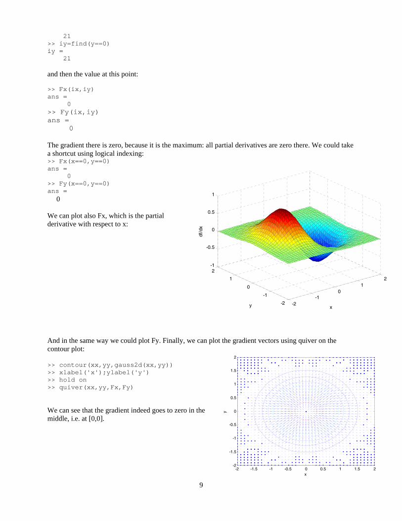
21 >> iy=find(y==0) iy = 21 and then the value at this point: >> Fx(ix,iy) ans = 0 >> Fy(ix,iy) ans = 0 The gradient there is zero, because it is the maximum: all partial derivatives are zero there. We could take a shortcut using logical indexing: >> Fx(x==0,y==0) ans = 0 >> Fy(x==0,y==0) ans = 0 We can plot also Fx, which is the partial derivative with respect to x: And in the same way we could plot Fy. Finally, we can plot the gradient vectors using quiver on the contour plot: >> contour(xx,yy,gauss2d(xx,yy)) >> xlabel('x');ylabel('y') >> hold on >> quiver(xx,yy,Fx,Fy) We can see that the gradient indeed goes to zero in the middle, i.e. at [0,0].

x

y

-2 -1.5 -1 -0.5 0 0.5 1 1.5 2-2

-1.5

-1

-0.5

0

0.5

1

1.5

2

-2-1

01

2

-2

-1

0

1

2-1

-0.5

0

0.5

1

xy

df/d

x

10

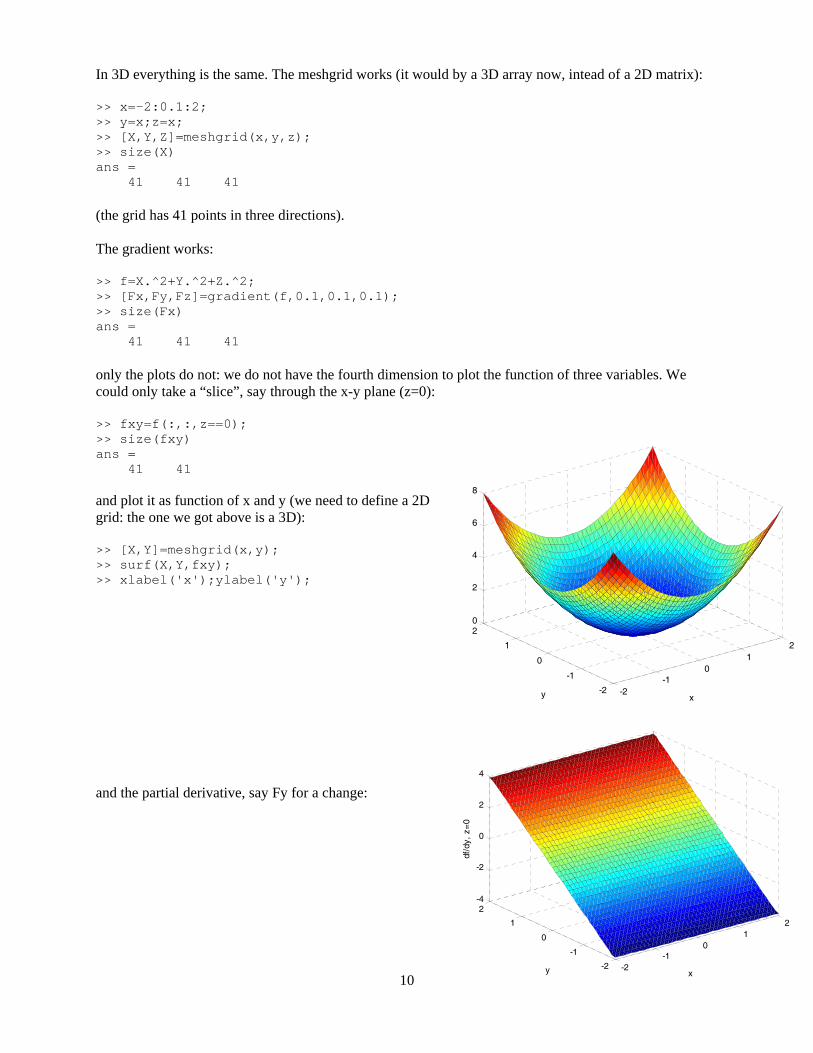
In 3D everything is the same. The meshgrid works (it would by a 3D array now, intead of a 2D matrix): >> x=-2:0.1:2; >> y=x;z=x; >> [X,Y,Z]=meshgrid(x,y,z); >> size(X) ans = 41 41 41 (the grid has 41 points in three directions). The gradient works: >> f=X.^2+Y.^2+Z.^2; >> [Fx,Fy,Fz]=gradient(f,0.1,0.1,0.1); >> size(Fx) ans = 41 41 41 only the plots do not: we do not have the fourth dimension to plot the function of three variables. We could only take a “slice”, say through the x-y plane (z=0): >> fxy=f(:,:,z==0); >> size(fxy) ans = 41 41 and plot it as function of x and y (we need to define a 2D grid: the one we got above is a 3D): >> [X,Y]=meshgrid(x,y); >> surf(X,Y,fxy); >> xlabel('x');ylabel('y'); and the partial derivative, say Fy for a change:

-2-1

01

2

-2

-1

0

1

20

2

4

6

8

xy

-2-1

01

2

-2

-1

0

1

2-4

-2

0

2

4

xy

df/d

y, z

=0

11

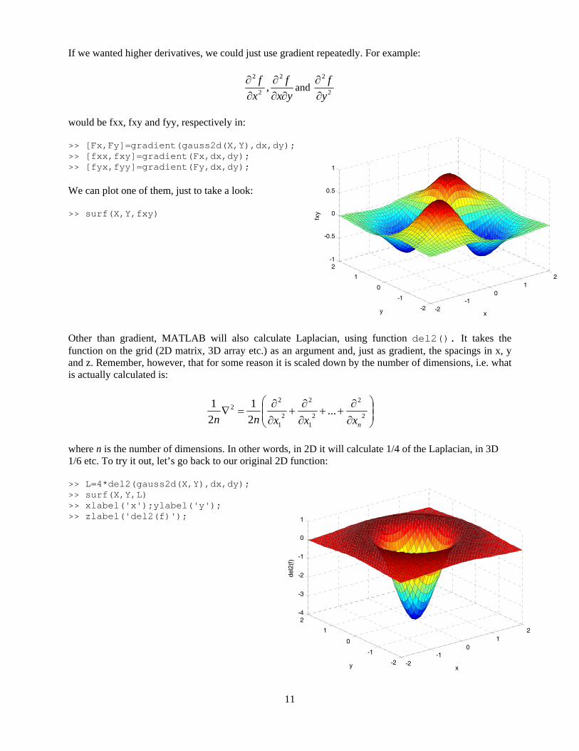
If we wanted higher derivatives, we could just use gradient repeatedly. For example:

yx

f

x

f

2

2

2

, and 2

2

y

f

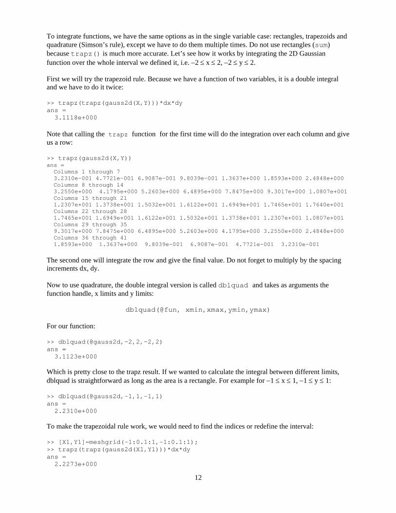
would be fxx, fxy and fyy, respectively in: >> [Fx,Fy]=gradient(gauss2d(X,Y),dx,dy); >> [fxx,fxy]=gradient(Fx,dx,dy); >> [fyx,fyy]=gradient(Fy,dx,dy); We can plot one of them, just to take a look: >> surf(X,Y,fxy) Other than gradient, MATLAB will also calculate Laplacian, using function del2(). It takes the function on the grid (2D matrix, 3D array etc.) as an argument and, just as gradient, the spacings in x, y and z. Remember, however, that for some reason it is scaled down by the number of dimensions, i.e. what is actually calculated is:

2

2

21

2

21

22 ...

2

1

2

1

nxxxnn where n is the number of dimensions. In other words, in 2D it will calculate 1/4 of the Laplacian, in 3D 1/6 etc. To try it out, let’s go back to our original 2D function: >> L=4*del2(gauss2d(X,Y),dx,dy); >> surf(X,Y,L) >> xlabel('x');ylabel('y'); >> zlabel('del2(f)');

-2-1

01

2

-2

-1

0

1

2-4

-3

-2

-1

0

1

xy

del2

(f)

-2-1

01

2

-2

-1

0

1

2-1

-0.5

0

0.5

1

xyfx

y

12

To integrate functions, we have the same options as in the single variable case: rectangles, trapezoids and quadrature (Simson’s rule), except we have to do them multiple times. Do not use rectangles (sum) because trapz() is much more accurate. Let’s see how it works by integrating the 2D Gaussian function over the whole interval we defined it, i.e. 2 x 2, 2 y 2. First we will try the trapezoid rule. Because we have a function of two variables, it is a double integral and we have to do it twice: >> trapz(trapz(gauss2d(X,Y)))*dx*dy ans = 3.1118e+000 Note that calling the trapz function for the first time will do the integration over each column and give us a row: >> trapz(gauss2d(X,Y)) ans = Columns 1 through 7 3.2310e-001 4.7721e-001 6.9087e-001 9.8039e-001 1.3637e+000 1.8593e+000 2.4848e+000 Columns 8 through 14 3.2550e+000 4.1795e+000 5.2603e+000 6.4895e+000 7.8475e+000 9.3017e+000 1.0807e+001 Columns 15 through 21 1.2307e+001 1.3738e+001 1.5032e+001 1.6122e+001 1.6949e+001 1.7465e+001 1.7640e+001 Columns 22 through 28 1.7465e+001 1.6949e+001 1.6122e+001 1.5032e+001 1.3738e+001 1.2307e+001 1.0807e+001 Columns 29 through 35 9.3017e+000 7.8475e+000 6.4895e+000 5.2603e+000 4.1795e+000 3.2550e+000 2.4848e+000 Columns 36 through 41 1.8593e+000 1.3637e+000 9.8039e-001 6.9087e-001 4.7721e-001 3.2310e-001 The second one will integrate the row and give the final value. Do not forget to multiply by the spacing increments dx, dy. Now to use quadrature, the double integral version is called dblquad and takes as arguments the function handle, x limits and y limits:

dblquad(@fun, xmin,xmax,ymin,ymax) For our function: >> dblquad(@gauss2d,-2,2,-2,2) ans = 3.1123e+000 Which is pretty close to the trapz result. If we wanted to calculate the integral between different limits, dblquad is straightforward as long as the area is a rectangle. For example for 1 x 1, 1 y 1: >> dblquad(@gauss2d,-1,1,-1,1) ans = 2.2310e+000 To make the trapezoidal rule work, we would need to find the indices or redefine the interval: >> [X1,Y1]=meshgrid(-1:0.1:1,-1:0.1:1); >> trapz(trapz(gauss2d(X1,Y1)))*dx*dy ans = 2.2273e+000

13

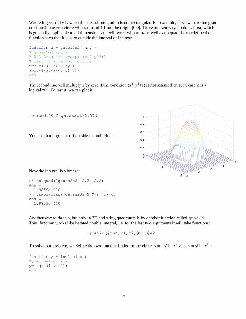
Where it gets tricky is when the area of integration is not rectangular. For example, if we want to integrate our function over a circle with radius of 1 from the origin [0,0]. There are two ways to do it. First, which is generally applicable to all dimensions and will work with trapz as well as dblquad, is to redefine the function such that it is zero outside the interval of interest: function z = gauss2d2( x,y ) % gauss2d( x,y ) % 2-D Gaussian z=exp(-(x^2+y^2)) % zero outside unit circle z=exp(-(x.*x+y.*y)) z=z.*((x.*x+y.*y)<1); end The second line will multiply z by zero if the condition (x2+y2<1) is not satisfied: in such case it is a logical “0”. To test it, we can plot it: >> mesh(X,Y,gauss2d2(X,Y)) You see that it got cut off outside the unit circle. Now the integral is a breeze: >> dblquad(@gauss2d2,-2,2,-2,2) ans = 1.9859e+000 >> trapz(trapz(gauss2d2(X,Y)))*dx*dy ans = 1.9809e+000 Another way to do this, but only in 2D and using quadrature is by another function called quad2d. This function works like iterated double integral, i.e. for the last two arguments it will take functions:

quad2d(@fun,x1,x2,@y1,@y2)

To solve our problem, we define the two function limits for the circle 21 xy and 21 xy : function y = lowlim( x ) %y = lowlim( x ) y=-sqrt(1-x.^2); end

-2-1

01

2

-2

-1

0

1

20

0.2

0.4

0.6

0.8

1

14

function y = uplim( x ) %y = upper( x ) y=sqrt(1-x.^2); end Then using quad2d our integral is: >> quad2d(@gauss2d,-1,1,@lowlim,@uplim) ans = 1.9859e+000 which is exactly the same number we got from dblquad. For 3D integrals you can use trapz three times (on a 3D meshgrid) or the function triplequad:

triplequad(@fun,x1,x2,y1,y2,z1,z2)

Again, if you integrate over some other shape than a rectabgular box, you let the function outside disappear. As an example, let us calculate the volume of a sphere with radius of 2. We write the following function: function val = sph2( x,y,z ) %shp2(x,y,z) shpere radius 2 val=(x.^2+y.^2+z.^2)<4; end And the volume would be the integral: >> triplequad(@sph2,-2,2,-2,2,-2,2) ans = 3.3510e+001

We can test this directly, because we know that the volume of a sphere is 3

3

4r

>> 4/3*pi*2^3 ans = 3.3510e+001 It checks.

15

Maxima and minima of multivariable functions. MATLAB has several built-in tools for finding minima of functions of many variables. Only minima: to find maximum you have to turn the problem into finding a minimum, which is easily done by turning the function into its negative. In other words, minimum of f(x,y) is the maximum of f(x,y). We will use the function aptly named fminsearch. It uses a so-called simples algorithm, which will evaluate the target function at different points, stepping toward the lower values until the values stop changing. This means, however, that it will find only a local minimum. It also requires that you input the initial point or “initial guess” of where the minimum should be: it will start its walk there. The basic syntax of fminsearch is a follows:

fminsearch(@fun,x0)

where @fun is the handle of the function to be minimized and x0 is the initial guess for the minimum. Note that x0 is only one variable. How can we use it for multi-variable functions? In fact, x0 can contain many variables, because it can be a vector. This, however, means that the function fun to be minimized has to be written as a function of a vector, e.g. [x y] for a two variable function, rather than explicitly two variables as we have been doing thus far. In addition, the function has to return a scalar as its first output argument. As an example, let’s find the maximum of the two dimensional Gaussian. To do that, the function has to be rewritten for vector input: function z = gauss2dvec(x) % gauss2dvec( x ) %x=x(1),y=x(2) % 2-D Gaussian z=exp(-(x^2+y^2)) % zero outside unit circle z=-exp(-(x(1).*x(1)+x(2).*x(2))); end Note that I also made it negative, because we will be searching for the maximum. Next I will take an initial guess, for example [-1,1]: >> x0=[-1,1]; and then call fminsearch: >> fminsearch(@gauss2dvec,x0) ans = 2.1024e-005 2.5485e-005 We know that the maximum is at [0,0]: this is pretty close. If we wanted more accurate answers, we would have to tighten the minimization criteria. That is done by defining options argument using optimset: options = optimset('TolX',1e-12); which sets more strict tolerance on x and then calling fminsearch with the new options, which go right after the initial guess in the argument list:

16

>> fminsearch(@gauss2dvec,x0,options) ans = 2.0186e-009 6.7110e-009 That is about as good as it will get. We can try to start from the true minimum: >> fminsearch(@gauss2dvec,[0 0],options) ans = 0 0 in which case it stays there. You can see that the exact result depends on the starting point and that it will always be approximate. What if we want to pass additional parameters to the function? The best way to do that is to define global variables. For example I may have another kind of a Gaussian function, which now depends aside from the variables x and y on three other parameters: a, b and c:

22 ycxbaez I would write the function as follows: function z = gauss2dabc(x) % gauss2dabc( x ) %x=x(1),y=x(2) % 2-D Gaussian z=a+b*exp(-c*(x^2+y^2)) % zero outside unit circle global a b c; z=a*exp(-b*(x(1)-c).*(x(1)-c)-x(2).*x(2)); z=-z; end and then define the global parameters (which may be universal constants, temperature, whatever you need them to be) before I call the function, most commonly from the MATLAB script. In fact, let us write a script for minimization of the function, which we will call minimization.m: % minimization clear all; global a b c; a=2; b=0.5; c=0.4; % x0=[1 1]; options=optimset('TolX',1e-9); xmin=fminsearch(@gauss2dabc,x0,options); disp('maximum is at:') disp(xmin); executing the script: >> minimization maximum is at: 4.0000e-001 -1.1807e-009

17

If I want to change the parameters, for example set c to 0.5: % minimization clear all; global a b c; a=2; b=0.5; c=-0.5; % x0=[1 1]; options=optimset('TolX',1e-9); xmin=fminsearch(@gauss2dabc,x0,options); disp('maximum is at:') disp(xmin); which will give me a different maximum: >> minimization maximum is at: -5.0000e-001 5.3604e-009 We can plot the function to check whether this is correct. For this, however, we would have to calculate the mesh grid of points and also rewrite the function script so that it takes two variables: x and y explicitly, not as a vector: function z = gauss2dabc_mesh(x,y) % gauss2dabc( x ) %x=x(1),y=x(2) % 2-D Gaussian z=a+b*exp(-c*(x^2+y^2)) % zero outside unit circle global a b c; z=a*exp(-b*(x-c).*(x-c)-y.*y); z=-z; end Then we can put the plot into our script: % minimization clear all; global a b c; a=2; b=0.5; c=-0.5; % x0=[1 1]; options=optimset('TolX',1e-9); xmin=fminsearch(@gauss2dabc,x0,options); disp('maximum is at:') disp(xmin); % x=-2:0.1:2; y=x; [xx,yy]=meshgrid(x,y); surf(xx,yy,gauss2dabc_mesh(xx,yy)); and call it:

18

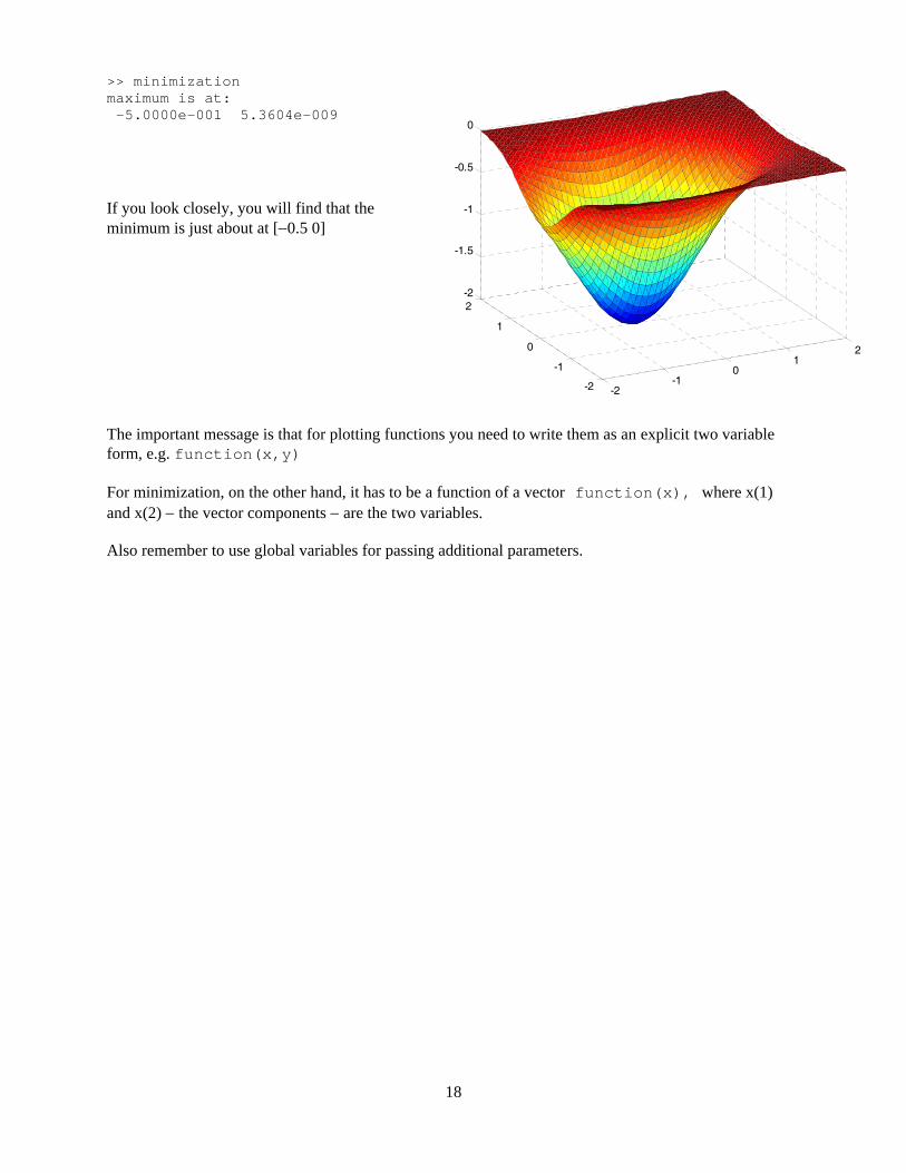
>> minimization maximum is at: -5.0000e-001 5.3604e-009 If you look closely, you will find that the minimum is just about at [0.5 0] The important message is that for plotting functions you need to write them as an explicit two variable form, e.g. function(x,y) For minimization, on the other hand, it has to be a function of a vector function(x), where x(1) and x(2) the vector components are the two variables. Also remember to use global variables for passing additional parameters.

-2-1

01

2

-2

-1

0

1

2-2

-1.5

-1

-0.5

0