Embed Size (px)
Citation preview
02.11.2017 Chapter 2 1
Fundamental Algorithms
Chapter 2: Advanced Heaps
Christian ScheidelerWS 2017

Contents
A heap implements a priority queue.We will consider the following heaps:• Binomial heap• Fibonacci heap• Radix heap
02.11.2017 Chapter 2 2
02.11.2017 Chapter 2 3
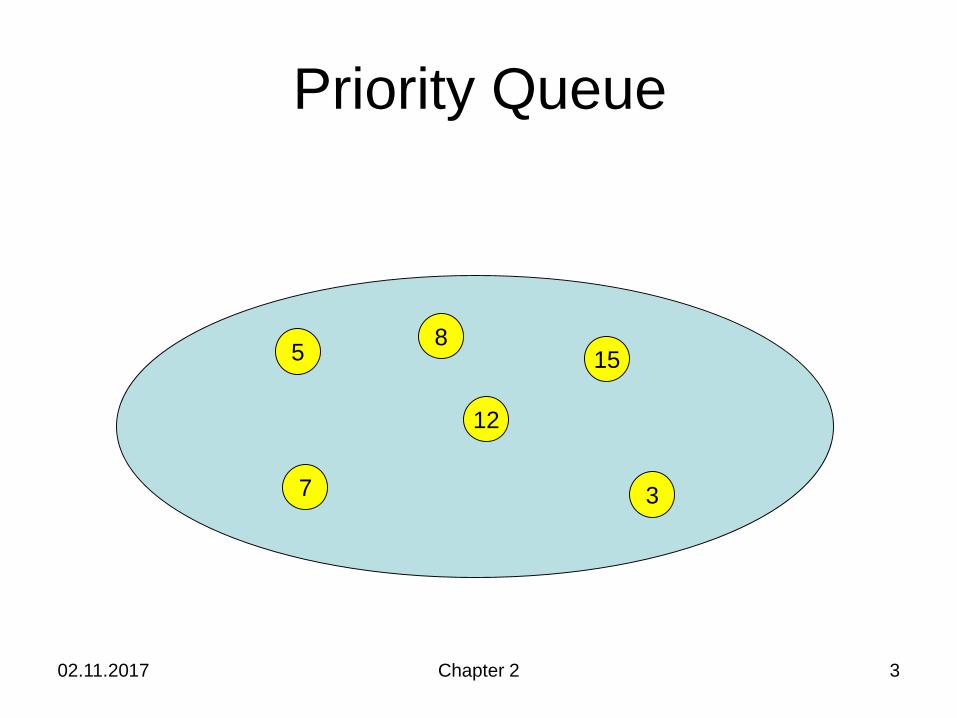
Priority Queue
5 8
12
15
37
02.11.2017 Chapter 2 4
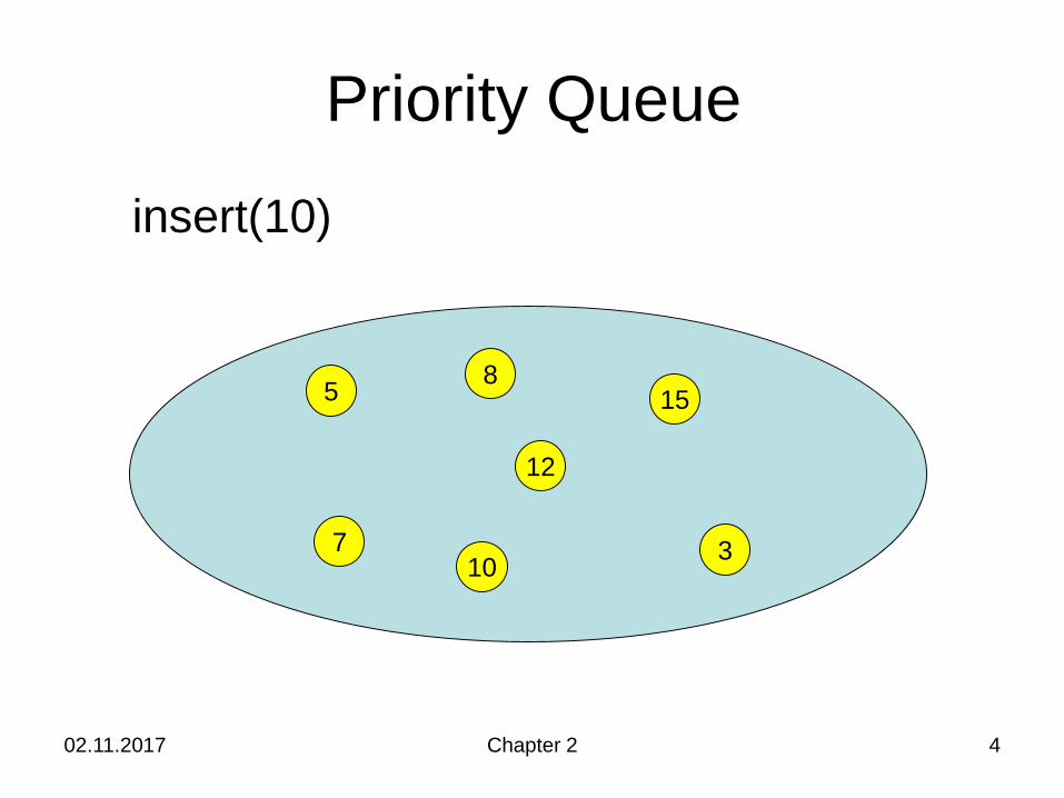
Priority Queue
5 8
12
15
37
insert(10)
10
02.11.2017 Chapter 2 5
Priority Queue
5 8
12
15
37
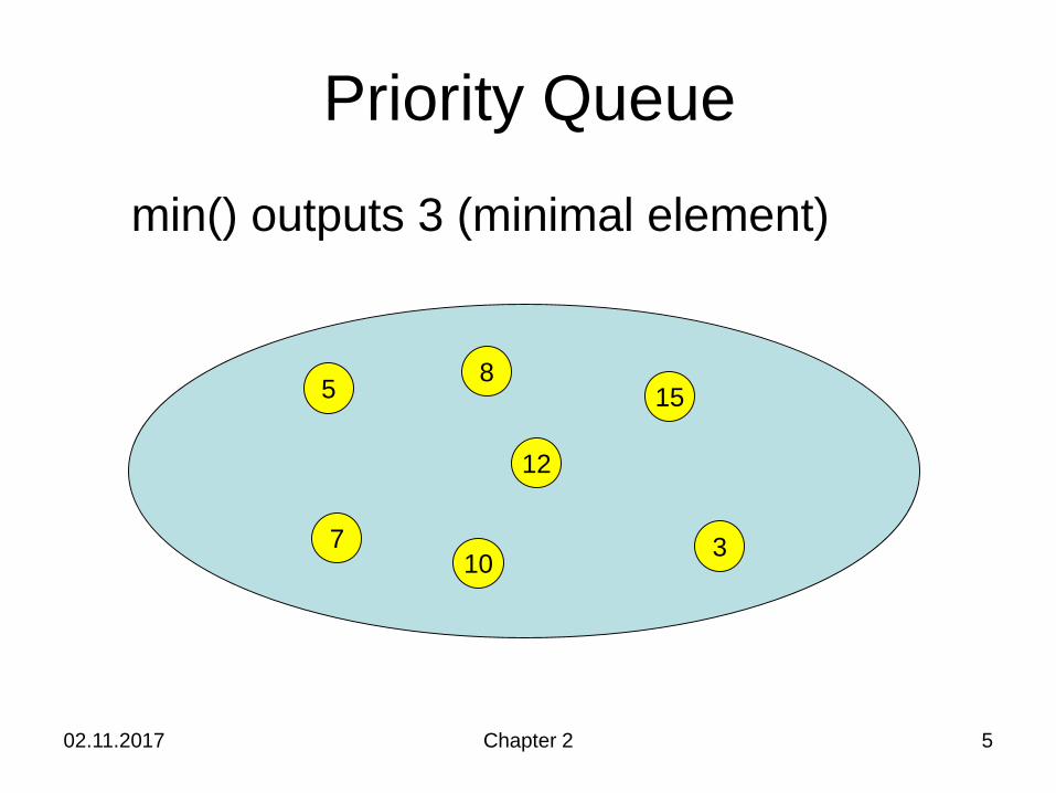
min() outputs 3 (minimal element)
10
02.11.2017 Chapter 2 6
Priority Queue
5 8
12
15
37
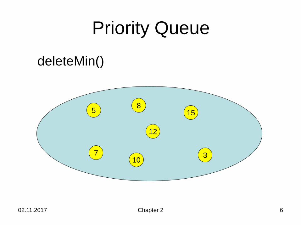
deleteMin()
10
02.11.2017 Chapter 2 7
Priority Queue
5 8
12
15
7
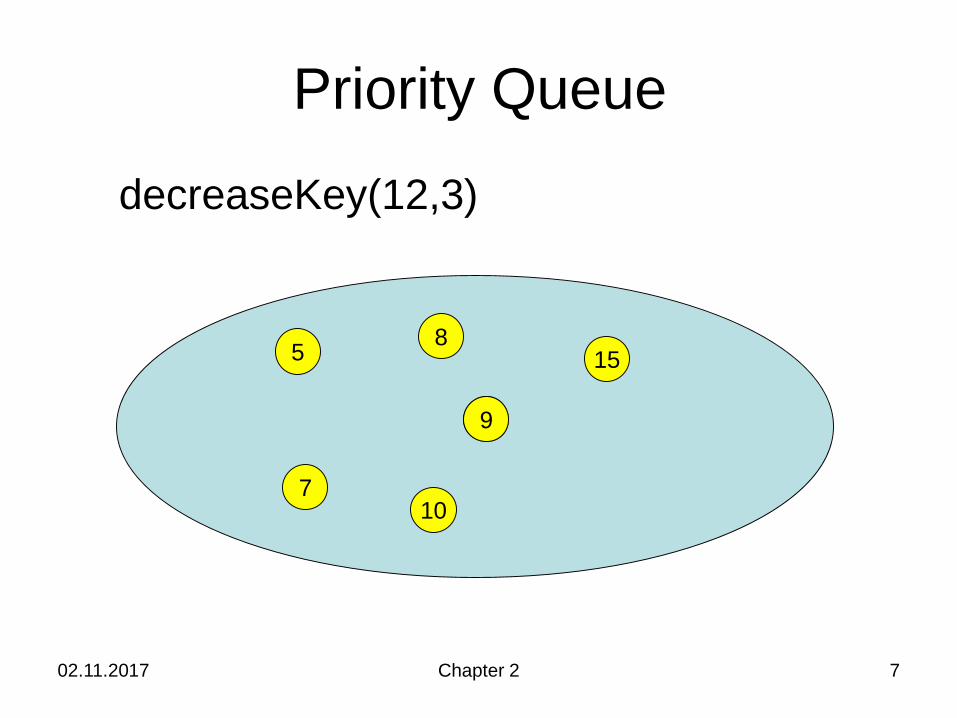
decreaseKey(12,3)
10
9
02.11.2017 Chapter 2 8
Priority Queue
5 815
7
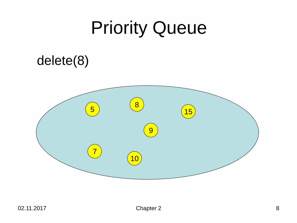
delete(8)
10
9
02.11.2017 Chapter 2 9
Priority Queue
5 8
15
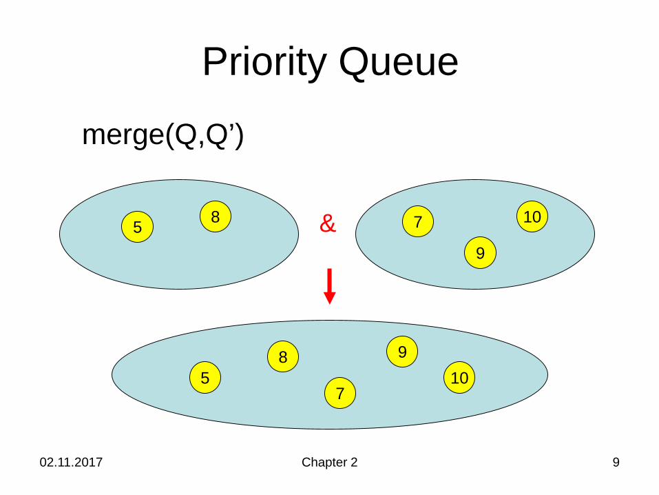
merge(Q,Q’)
7
9
10
58
7
910
&
02.11.2017 Chapter 2 10
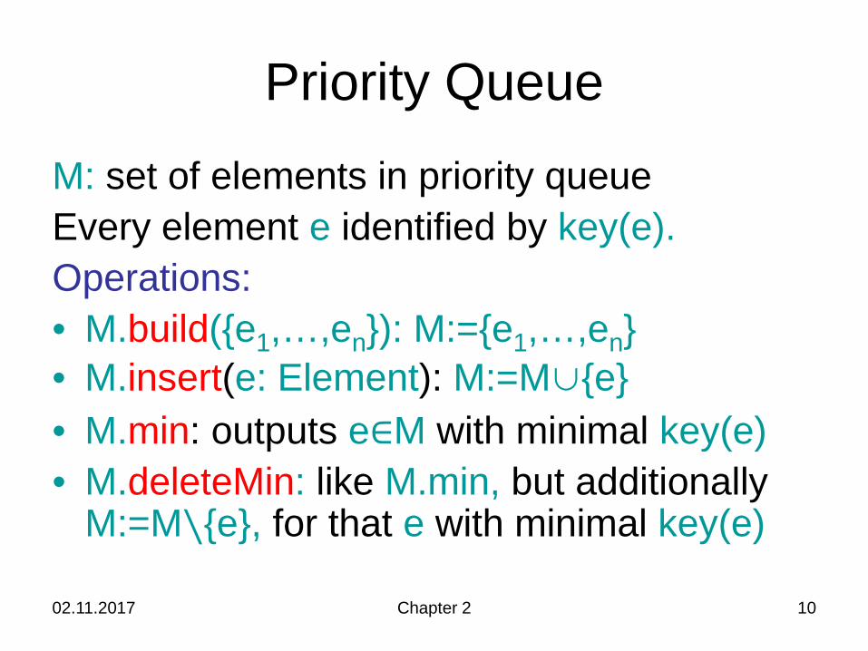
Priority QueueM: set of elements in priority queueEvery element e identified by key(e).Operations:• M.build({e1,…,en}): M:={e1,…,en}• M.insert(e: Element): M:=M∪{e}• M.min: outputs e∈M with minimal key(e)• M.deleteMin: like M.min, but additionally
M:=M∖{e}, for that e with minimal key(e)
02.11.2017 Chapter 2 11
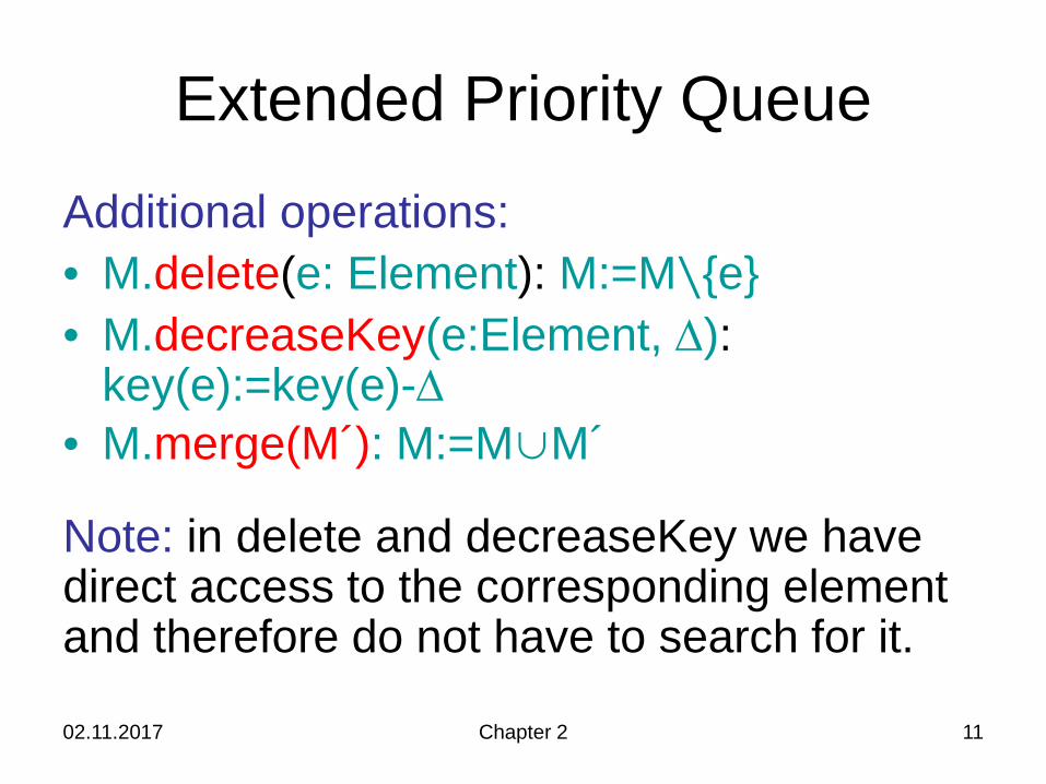
Extended Priority QueueAdditional operations:• M.delete(e: Element): M:=M∖{e}• M.decreaseKey(e:Element, ∆):
key(e):=key(e)-∆• M.merge(M´): M:=M∪M´
Note: in delete and decreaseKey we havedirect access to the corresponding elementand therefore do not have to search for it.

Why Priority Queues?
• Sorting: Heapsort• Shortest paths: Dijkstra´s algorithm• Minimum spanning trees: Prim´s algorithm• Job scheduling: EDF (earliest deadline
first)
02.11.2017 Chapter 2 12
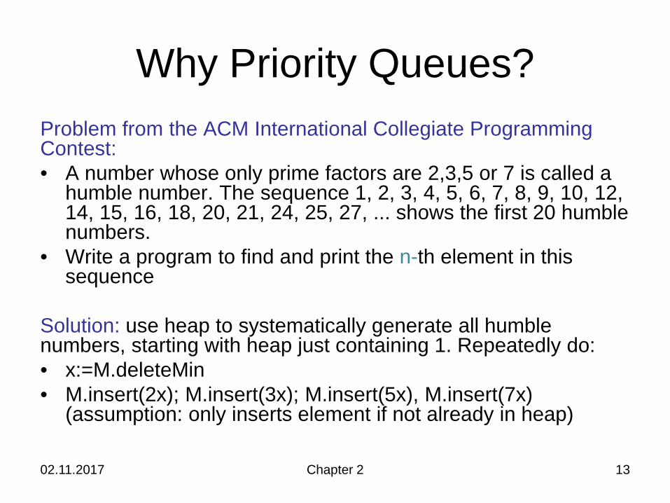
Why Priority Queues?Problem from the ACM International Collegiate Programming Contest:• A number whose only prime factors are 2,3,5 or 7 is called a
humble number. The sequence 1, 2, 3, 4, 5, 6, 7, 8, 9, 10, 12, 14, 15, 16, 18, 20, 21, 24, 25, 27, ... shows the first 20 humble numbers.
• Write a program to find and print the n-th element in this sequence
Solution: use heap to systematically generate all humble numbers, starting with heap just containing 1. Repeatedly do:• x:=M.deleteMin• M.insert(2x); M.insert(3x); M.insert(5x), M.insert(7x)
(assumption: only inserts element if not already in heap)
02.11.2017 Chapter 2 13
02.11.2017 Chapter 2 14
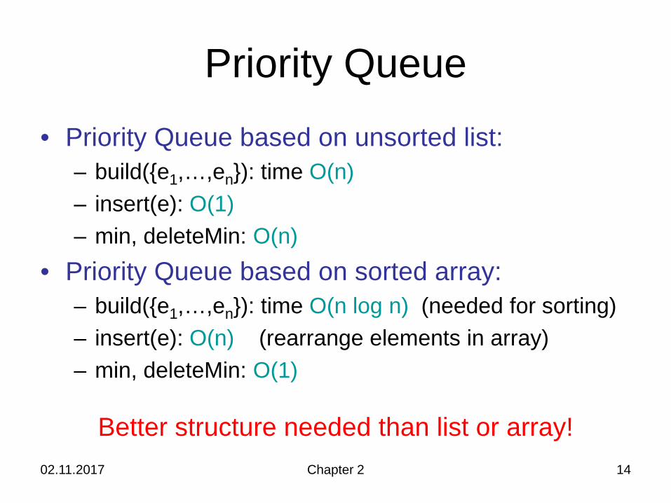
Priority Queue• Priority Queue based on unsorted list:
– build({e1,…,en}): time O(n)– insert(e): O(1) – min, deleteMin: O(n)
• Priority Queue based on sorted array:– build({e1,…,en}): time O(n log n) (needed for sorting)– insert(e): O(n) (rearrange elements in array)– min, deleteMin: O(1)
Better structure needed than list or array!
02.11.2017 Chapter 2 15
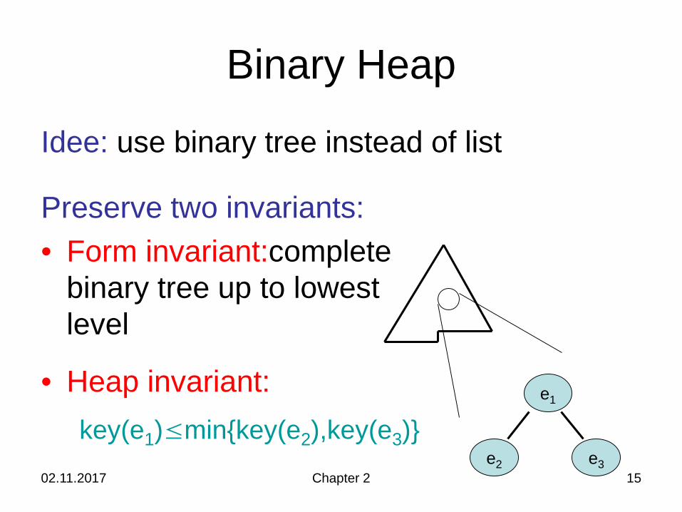
Binary Heap
Idee: use binary tree instead of list
Preserve two invariants:• Form invariant:complete
binary tree up to lowest level
• Heap invariant: e1
e2 e3
key(e1)≤min{key(e2),key(e3)}
02.11.2017 Chapter 2 16
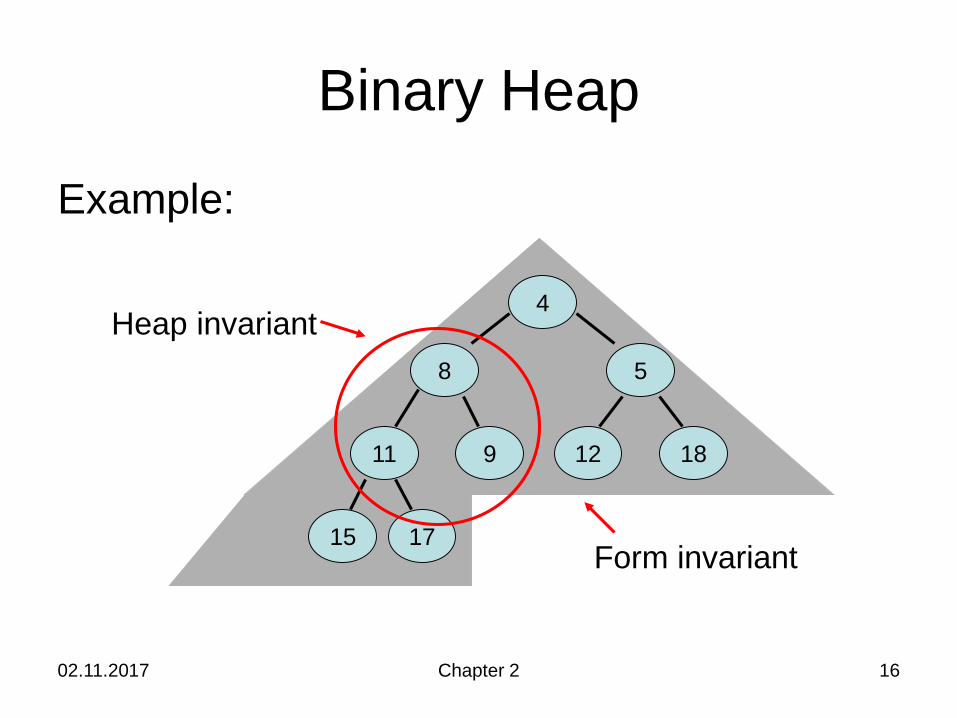
Binary Heap
Example:
4
8 5
11 9 12 18
15 17Form invariant
Heap invariant
02.11.2017 Chapter 2 17
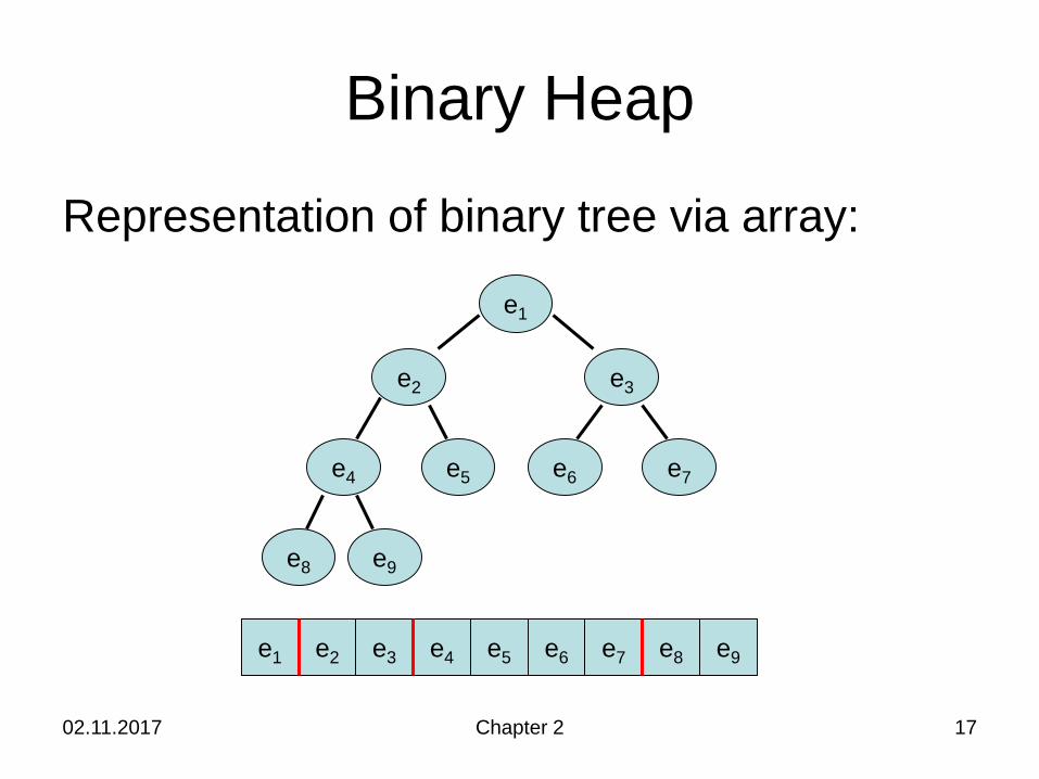
Binary Heap
Representation of binary tree via array:
e1
e2 e3
e4 e5 e6 e7
e8 e9
e1 e2 e3 e4 e5 e6 e7 e8 e9e3
02.11.2017 Chapter 2 18
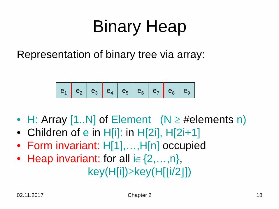
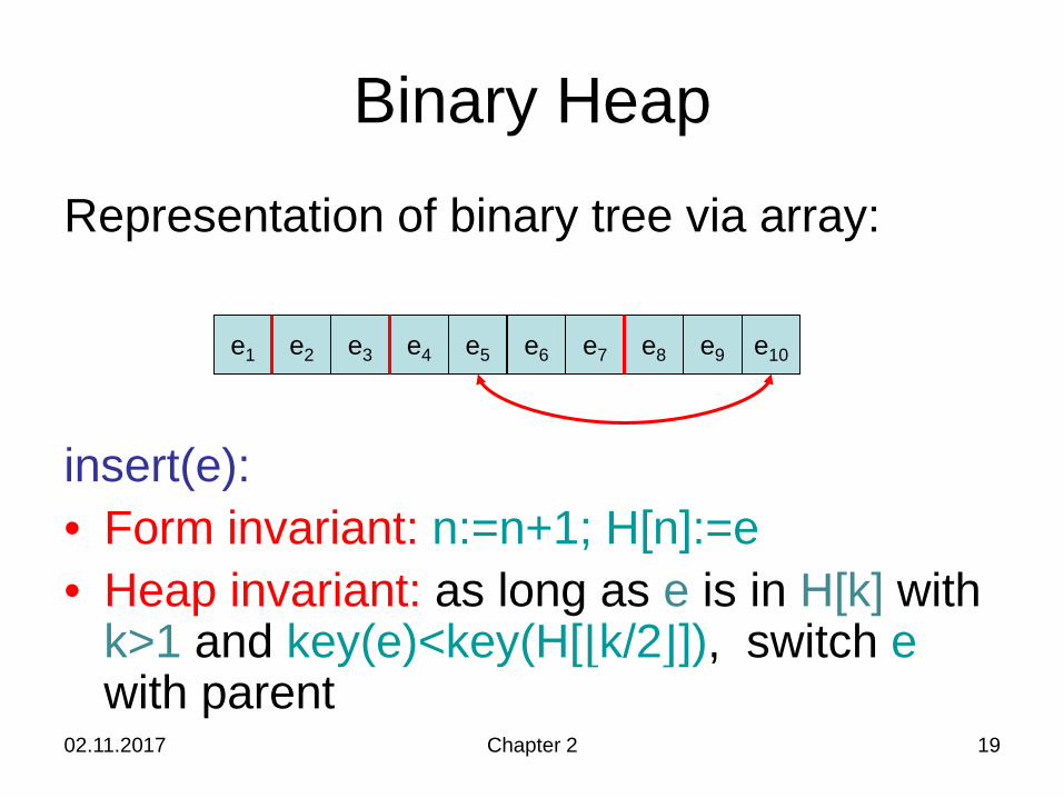
Binary HeapRepresentation of binary tree via array:
• H: Array [1..N] of Element (N ≥ #elements n)• Children of e in H[i]: in H[2i], H[2i+1]• Form invariant: H[1],…,H[n] occupied• Heap invariant: for all i∈{2,…,n},
key(H[i])≥key(H[⌊i/2⌋])
e1 e2 e3 e4 e5 e6 e7 e8 e9e3
02.11.2017 Chapter 2 19
Binary HeapRepresentation of binary tree via array:
insert(e):• Form invariant: n:=n+1; H[n]:=e• Heap invariant: as long as e is in H[k] with
k>1 and key(e)<key(H[⌊k/2⌋]), switch ewith parent
e1 e2 e3 e4 e5 e6 e7 e8 e9e3 e10
02.11.2017 Chapter 2 20
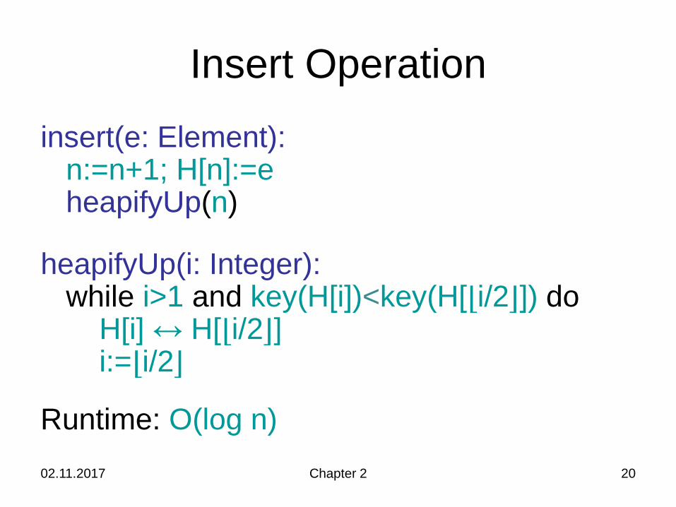
Insert Operationinsert(e: Element):
n:=n+1; H[n]:=eheapifyUp(n)
heapifyUp(i: Integer):while i>1 and key(H[i])<key(H[⌊i/2⌋]) do
H[i] ↔ H[⌊i/2⌋]i:=⌊i/2⌋
Runtime: O(log n)
02.11.2017 Chapter 2 21
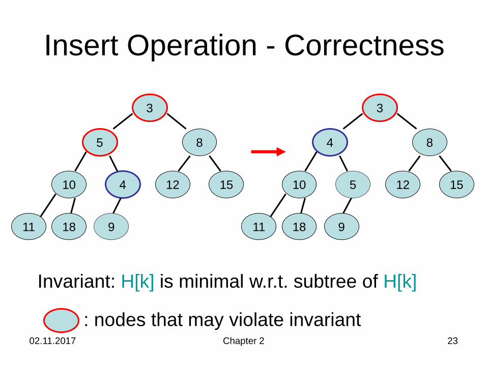
Insert Operation - Correctness
3
5 8
10 9 12 15
11 18
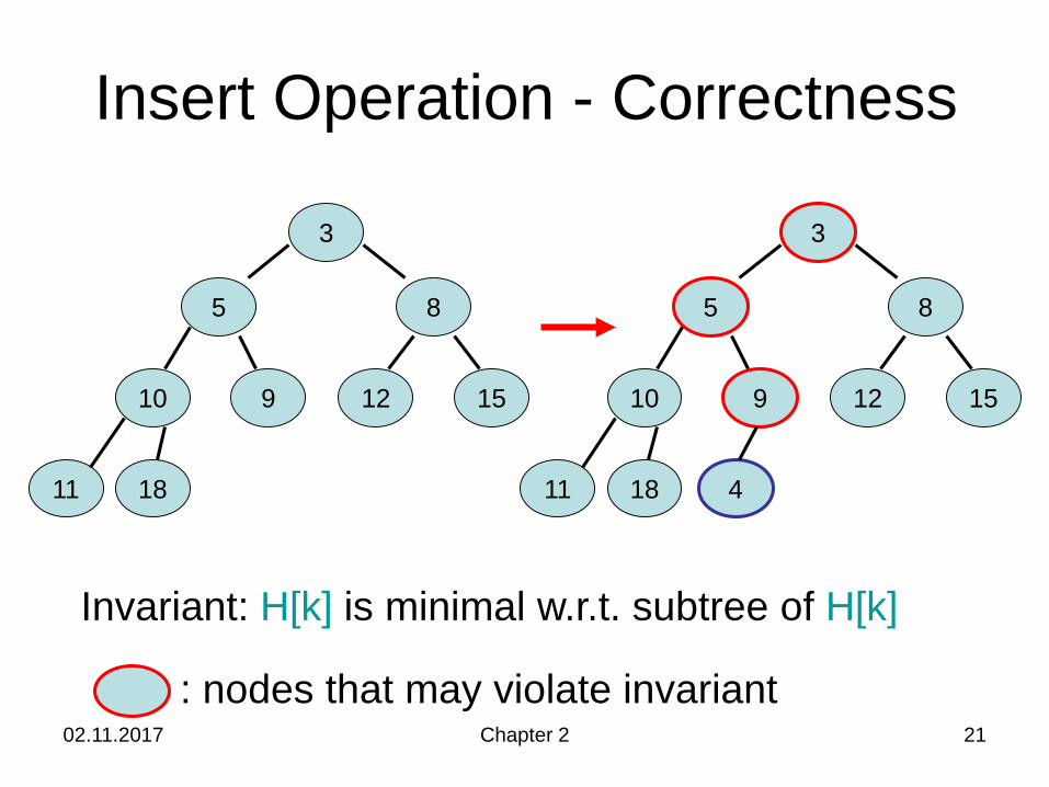
Invariant: H[k] is minimal w.r.t. subtree of H[k]
: nodes that may violate invariant
3
5 8
10 9 12 15
11 18 4
02.11.2017 Chapter 2 22
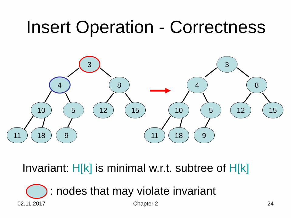
Insert Operation - Correctness
3
5 8
10 9 12 15
11 18 4
3
5 8
10 4 12 15
11 18 9
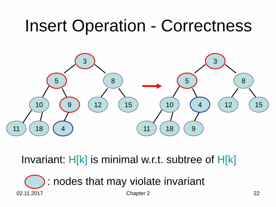
Invariant: H[k] is minimal w.r.t. subtree of H[k]
: nodes that may violate invariant
02.11.2017 Chapter 2 23
Insert Operation - Correctness
3
5 8
10 4 12 15
11 18 9
3
4 8
10 5 12 15
11 18 9
Invariant: H[k] is minimal w.r.t. subtree of H[k]
: nodes that may violate invariant
02.11.2017 Chapter 2 24
Insert Operation - Correctness
3
4 8
10 5 12 15
11 18 9
3
4 8
10 5 12 15
11 18 9
Invariant: H[k] is minimal w.r.t. subtree of H[k]
: nodes that may violate invariant
02.11.2017 Chapter 2 25
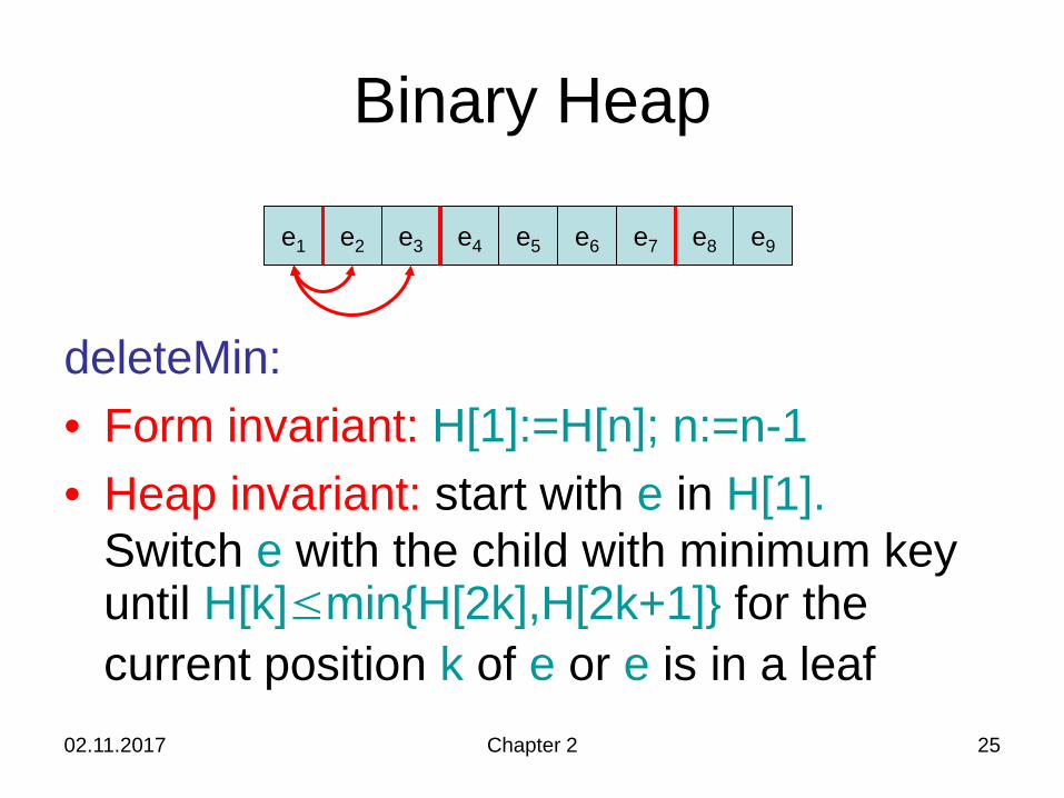
Binary Heap
deleteMin:• Form invariant: H[1]:=H[n]; n:=n-1• Heap invariant: start with e in H[1].
Switch e with the child with minimum key until H[k]≤min{H[2k],H[2k+1]} for the current position k of e or e is in a leaf
e1 e2 e3 e4 e5 e6 e7 e8 e9e3
02.11.2017 Chapter 2 26
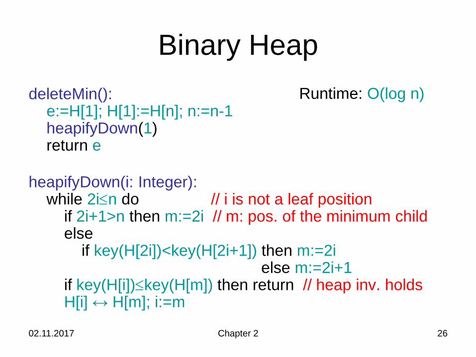
Binary HeapdeleteMin():
e:=H[1]; H[1]:=H[n]; n:=n-1heapifyDown(1)return e
heapifyDown(i: Integer):while 2i≤n do // i is not a leaf position
if 2i+1>n then m:=2i // m: pos. of the minimum childelse
if key(H[2i])<key(H[2i+1]) then m:=2ielse m:=2i+1
if key(H[i])≤key(H[m]) then return // heap inv. holdsH[i] ↔ H[m]; i:=m
Runtime: O(log n)
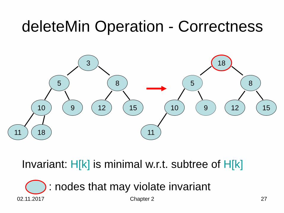
02.11.2017 Chapter 2 27
deleteMin Operation - Correctness
3
5 8
10 9 12 15
11 18
5 8
10 9 12 15
11
18
Invariant: H[k] is minimal w.r.t. subtree of H[k]
: nodes that may violate invariant
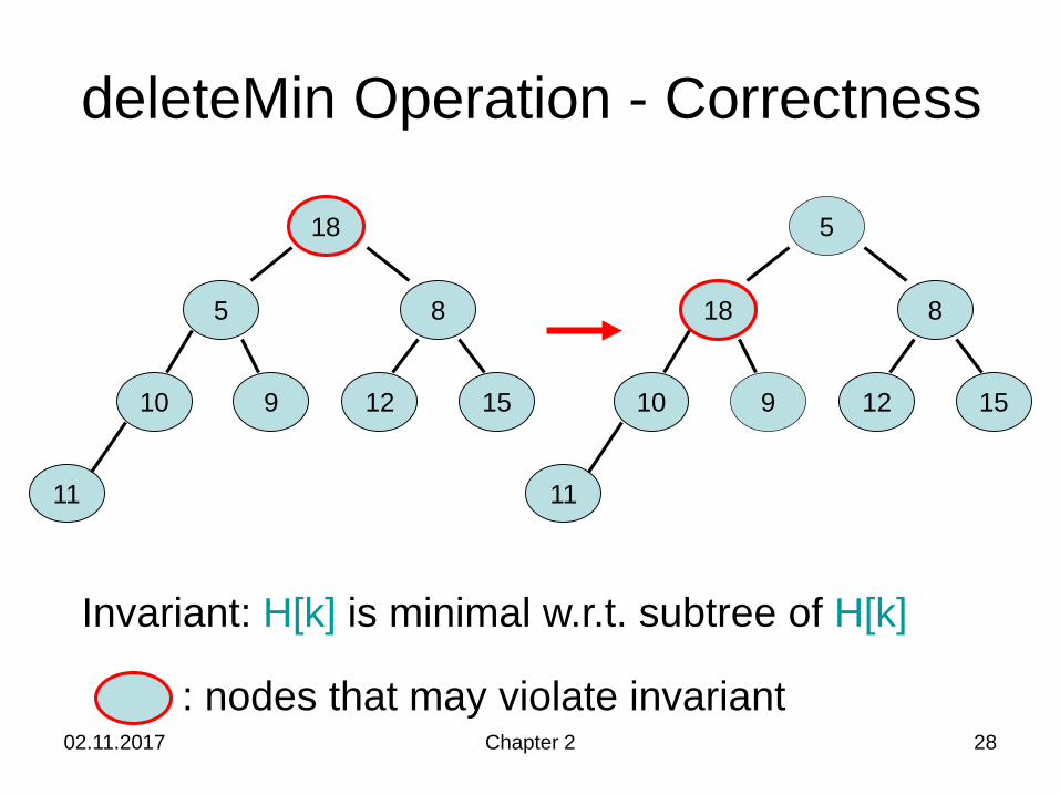
02.11.2017 Chapter 2 28
deleteMin Operation - Correctness
5 8
10 9 12 15
11
5
8
10 9 12 15
11
18
18
Invariant: H[k] is minimal w.r.t. subtree of H[k]
: nodes that may violate invariant
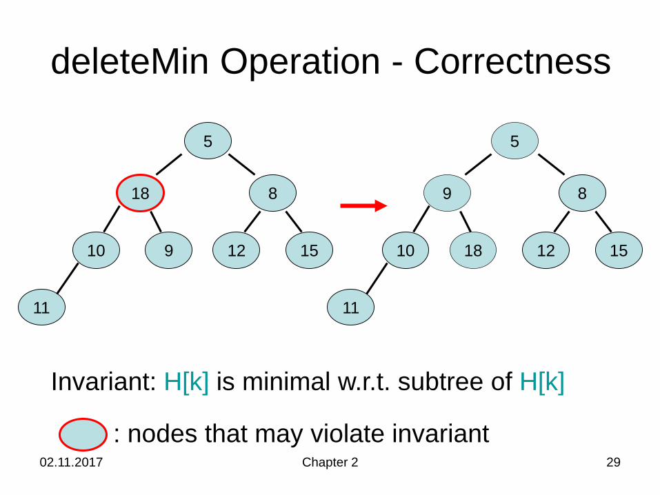
02.11.2017 Chapter 2 29
deleteMin Operation - Correctness
5
8
10 9 12 15
11
5
8
10
9
12 15
11
18
18
Invariant: H[k] is minimal w.r.t. subtree of H[k]
: nodes that may violate invariant
02.11.2017 Chapter 2 30
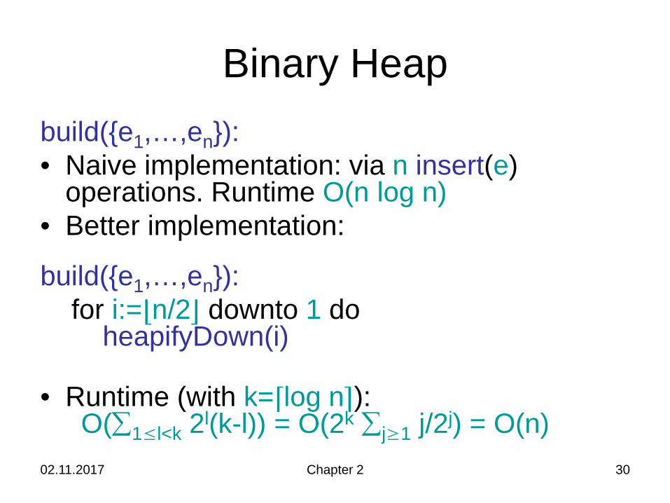
Binary Heapbuild({e1,…,en}):• Naive implementation: via n insert(e)
operations. Runtime O(n log n)• Better implementation:
build({e1,…,en}):for i:=⌊n/2⌋ downto 1 do
heapifyDown(i)
• Runtime (with k=⌈log n⌉):O(∑1≤l<k 2l(k-l)) = O(2k ∑j≥1 j/2j) = O(n)
02.11.2017 Chapter 2 31
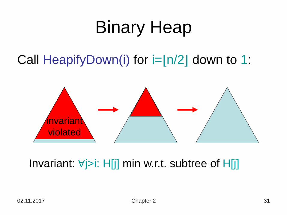
Binary Heap
Call HeapifyDown(i) for i=⌊n/2⌋ down to 1:
Invariant: ∀j>i: H[j] min w.r.t. subtree of H[j]
invariantviolated
02.11.2017 Chapter 2 32
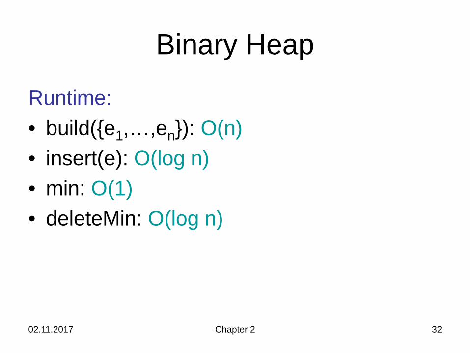
Binary Heap
Runtime:• build({e1,…,en}): O(n)• insert(e): O(log n)• min: O(1)• deleteMin: O(log n)
02.11.2017 Chapter 2 33
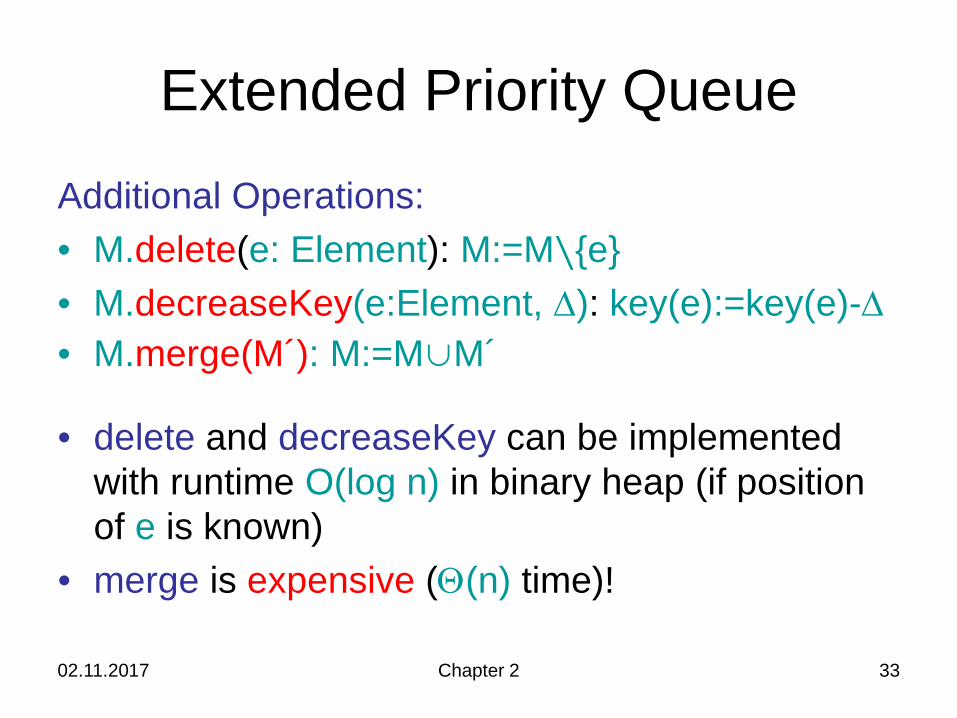
Extended Priority QueueAdditional Operations:• M.delete(e: Element): M:=M∖{e}• M.decreaseKey(e:Element, ∆): key(e):=key(e)-∆• M.merge(M´): M:=M∪M´
• delete and decreaseKey can be implemented with runtime O(log n) in binary heap (if position of e is known)
• merge is expensive (Θ(n) time)!
02.11.2017 Chapter 2 34
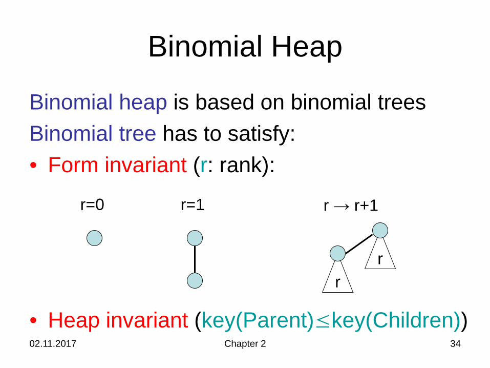
Binomial Heap
Binomial heap is based on binomial treesBinomial tree has to satisfy:• Form invariant (r: rank):
• Heap invariant (key(Parent)≤key(Children))
r=0 r=1 r → r+1
rr
02.11.2017 Chapter 2 35
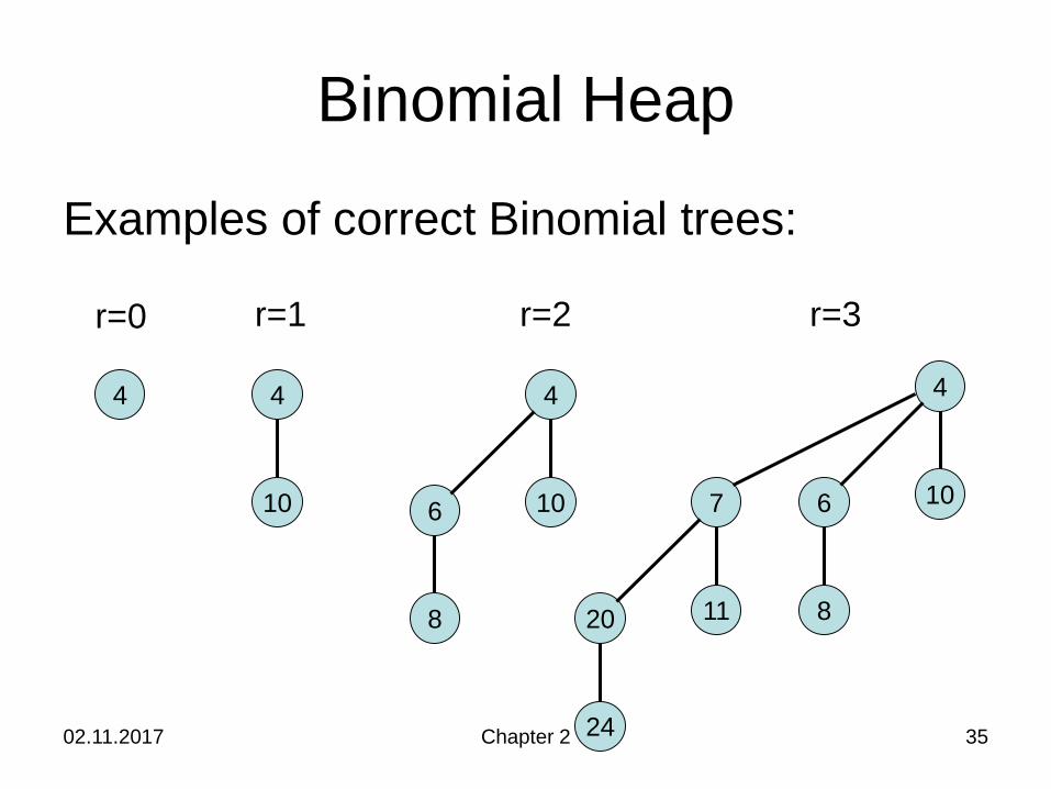
Binomial Heap
Examples of correct Binomial trees:
4 4
10
4
106
8
4
106
8
7
1120
24
r=0 r=1 r=2 r=3
02.11.2017 Chapter 2 36
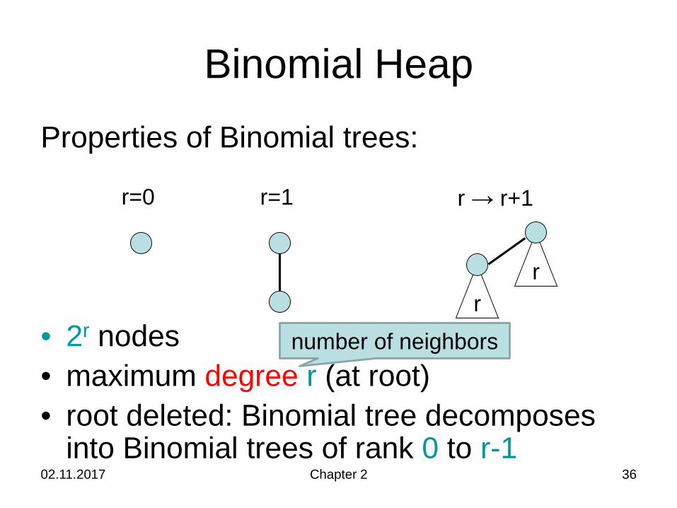
Binomial HeapProperties of Binomial trees:
• 2r nodes• maximum degree r (at root)• root deleted: Binomial tree decomposes
into Binomial trees of rank 0 to r-1
r=0 r=1 r → r+1
rr
number of neighbors
02.11.2017 Chapter 2 37
Binomial Heap
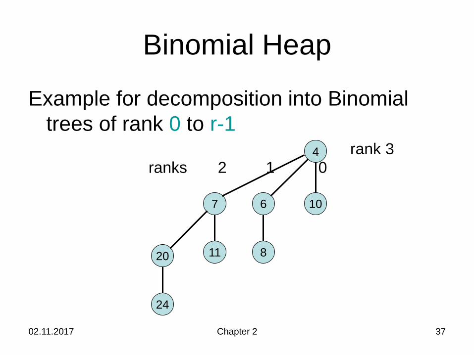
Example for decomposition into Binomial trees of rank 0 to r-1
4
106
8
7
1120
24
rank 3ranks 2 1 0
02.11.2017 Chapter 2 38
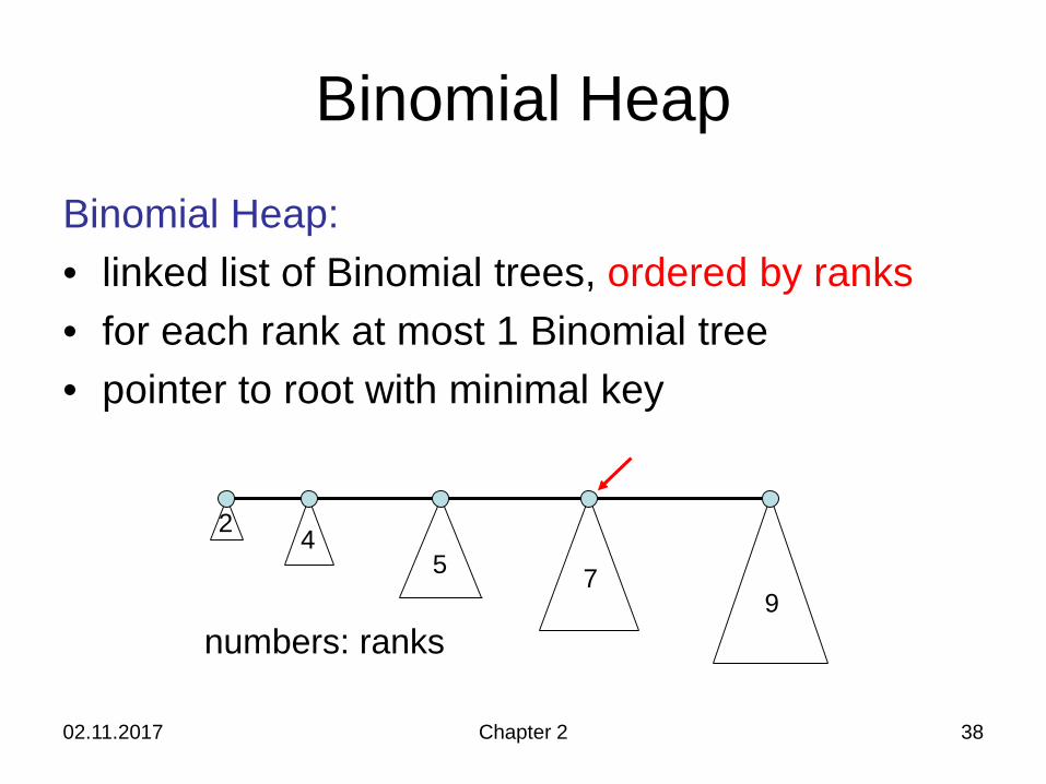
Binomial HeapBinomial Heap:• linked list of Binomial trees, ordered by ranks• for each rank at most 1 Binomial tree• pointer to root with minimal key
2 45 7
9numbers: ranks
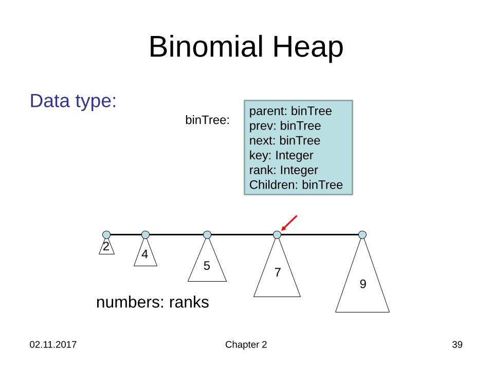
Binomial Heap
02.11.2017 Chapter 2 39
Data type:
2 45 7
9numbers: ranks
parent: binTreeprev: binTreenext: binTreekey: Integerrank: IntegerChildren: binTree
binTree:
02.11.2017 Chapter 2 40
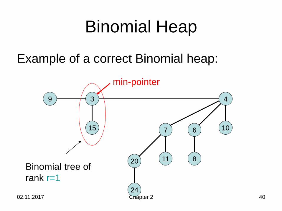
Binomial Heap
Example of a correct Binomial heap:
4
106
8
7
1120
24
9 3
15
min-pointer
Binomial tree ofrank r=1
02.11.2017 Chapter 2 41
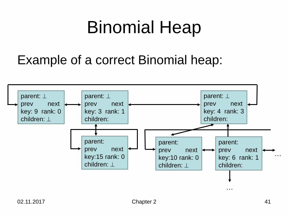
Binomial Heap
Example of a correct Binomial heap:
parent: ⊥prev nextkey: 9 rank: 0children: ⊥
…
…
parent: ⊥prev nextkey: 3 rank: 1children:
parent: prev nextkey:15 rank: 0children: ⊥
parent: ⊥prev nextkey: 4 rank: 3children:
parent: prev nextkey:10 rank: 0children: ⊥
parent: prev nextkey: 6 rank: 1children:
02.11.2017 Chapter 2 42
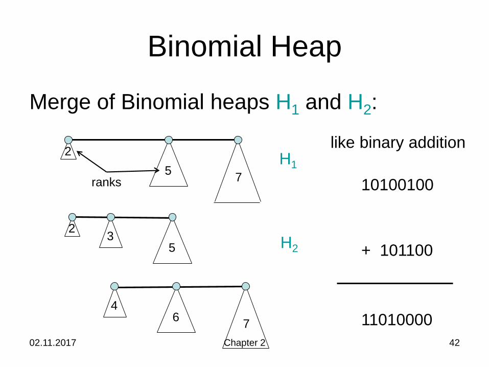
Binomial Heap
Merge of Binomial heaps H1 and H2:
25 7
2 35
46 7
H1
H2
10100100
+ 101100
11010000
like binary addition
ranks
02.11.2017 Chapter 2 43
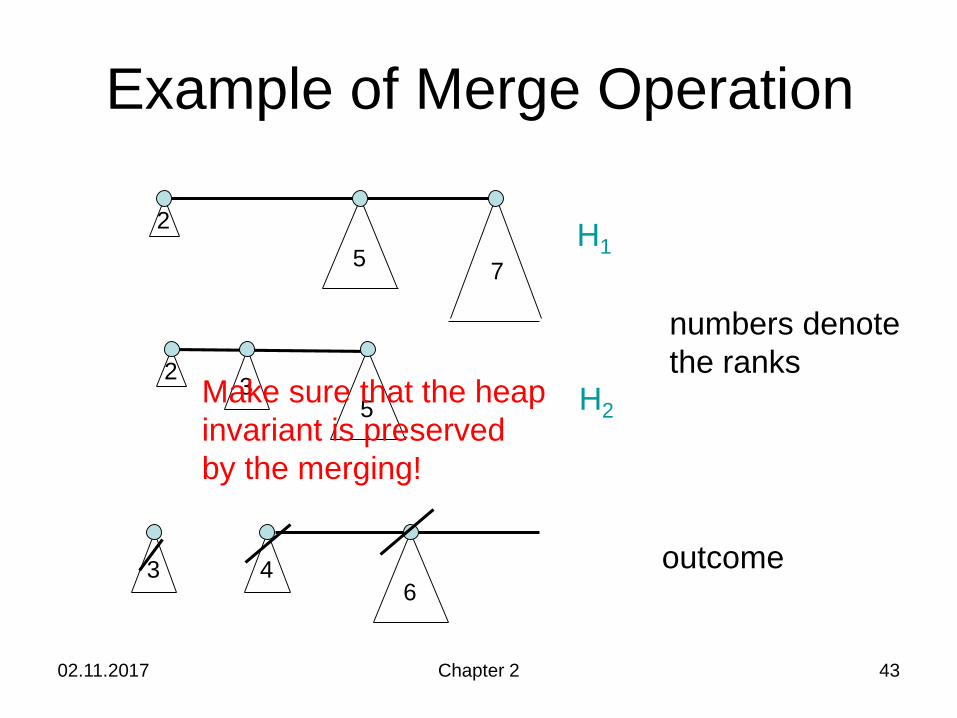
Example of Merge Operation
25
2 35
7H1
H2
36
4
Make sure that the heap invariant is preservedby the merging!
outcome
numbers denotethe ranks
02.11.2017 Chapter 2 44
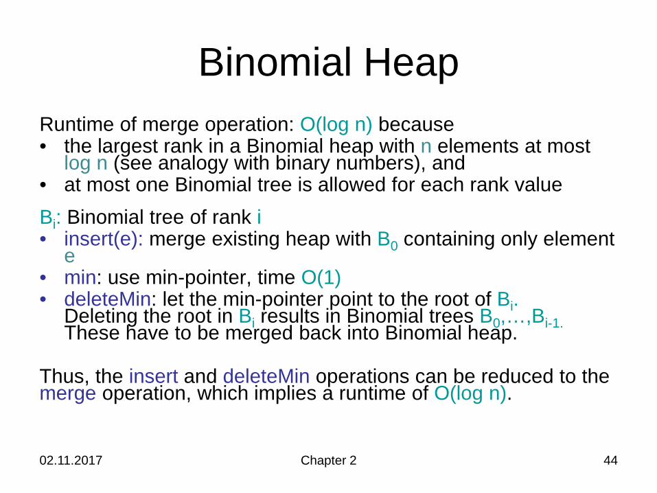
Binomial HeapRuntime of merge operation: O(log n) because• the largest rank in a Binomial heap with n elements at most
log n (see analogy with binary numbers), and• at most one Binomial tree is allowed for each rank valueBi: Binomial tree of rank i• insert(e): merge existing heap with B0 containing only element
e• min: use min-pointer, time O(1)• deleteMin: let the min-pointer point to the root of Bi.Deleting the root in Bi results in Binomial trees B0,…,Bi-1.These have to be merged back into Binomial heap.
Thus, the insert and deleteMin operations can be reduced to themerge operation, which implies a runtime of O(log n).
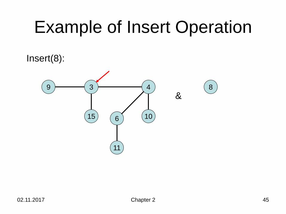
Example of Insert Operation
02.11.2017 Chapter 2 45
4
106
11
9 3
15
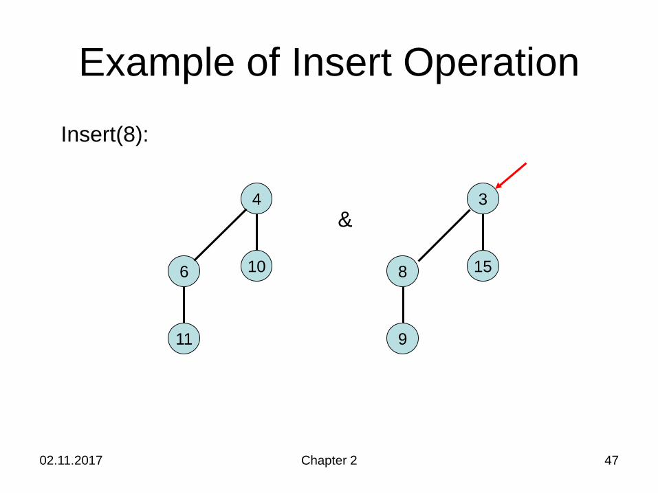
Insert(8):
&8
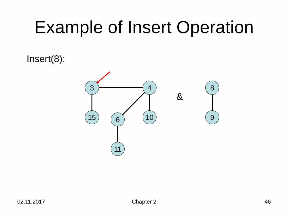
Example of Insert Operation
02.11.2017 Chapter 2 46
4
106
11
9
3
15
Insert(8):
&8
Example of Insert Operation
02.11.2017 Chapter 2 47
4
106
11 9
3
15
Insert(8):
&
8
Example of Insert Operation
02.11.2017 Chapter 2 48
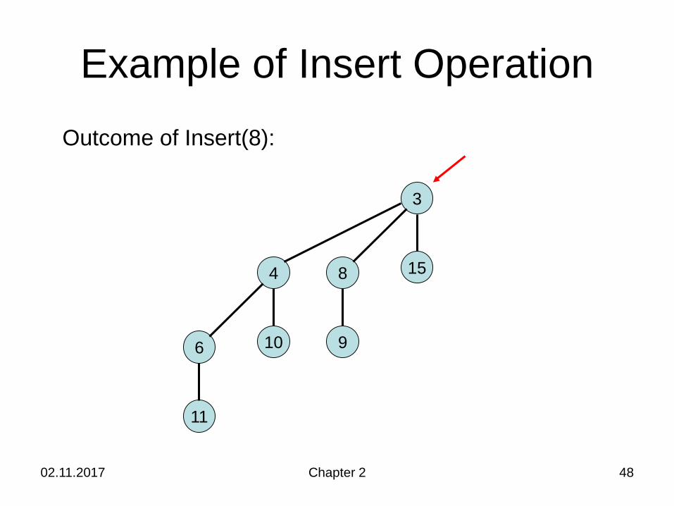
Outcome of Insert(8):
3
158
9
4
106
11
02.11.2017 Chapter 2 49
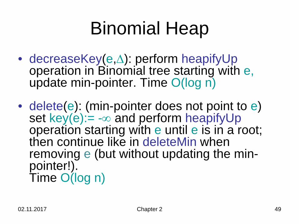
Binomial Heap• decreaseKey(e,∆): perform heapifyUp
operation in Binomial tree starting with e, update min-pointer. Time O(log n)
• delete(e): (min-pointer does not point to e) set key(e):= -∞ and perform heapifyUpoperation starting with e until e is in a root; then continue like in deleteMin whenremoving e (but without updating the min-pointer!).Time O(log n)

Example of decreaseKey
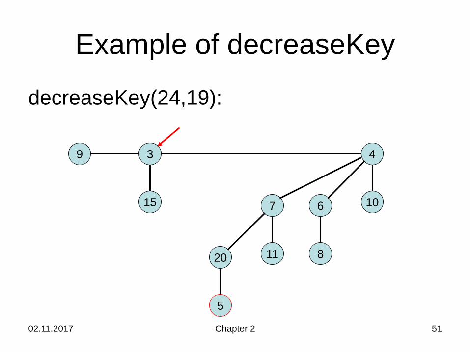
decreaseKey(24,19):
02.11.2017 Chapter 2 50
4
106
8
7
1120
24
9 3
15
Example of decreaseKey
decreaseKey(24,19):
02.11.2017 Chapter 2 51
4
106
8
7
1120
5
9 3
15

Example of decreaseKey
decreaseKey(24,19):
02.11.2017 Chapter 2 52
4
106
8
7
11
20
5
9 3
15
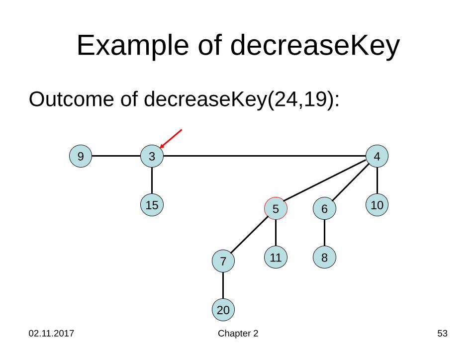
Example of decreaseKey
Outcome of decreaseKey(24,19):
02.11.2017 Chapter 2 53
4
106
8
5
117
20
9 3
15
02.11.2017 Chapter 2 54
Fibonacci Heap
• Based on Binomial trees, but it allows lazy merge and lazy delete.
• Lazy merge: no merging of Binomial trees of the same rank during merge, only concatenation of the two lists
• Lazy delete: creates incomplete Binomial trees
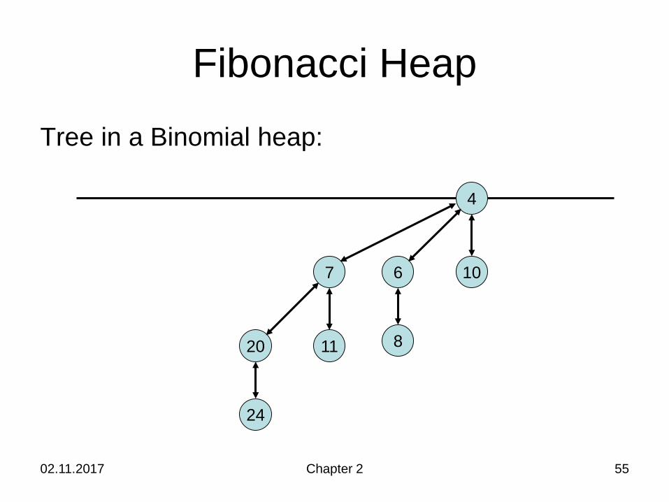
02.11.2017 Chapter 2 55
Fibonacci HeapTree in a Binomial heap:
4
106
8
7
1120
24
02.11.2017 Chapter 2 56
Fibonacci HeapTree in a Fibonacci heap:
4
106
8
7
1120
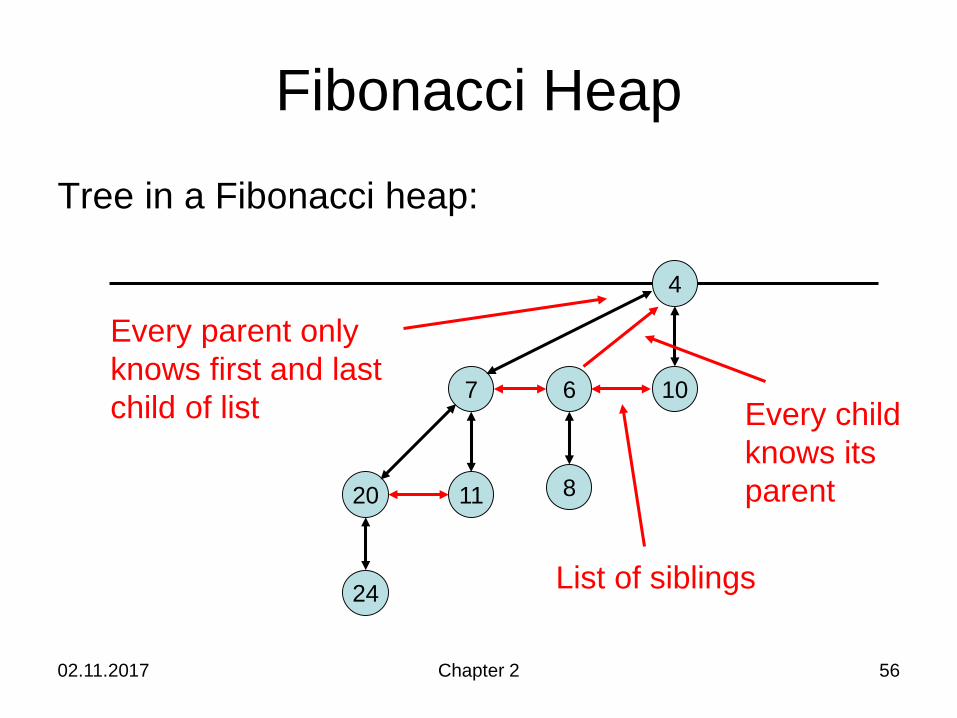
24 List of siblings
Every parent only knows first and last child of list Every child
knows itsparent
02.11.2017 Chapter 2 57
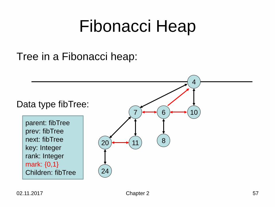
Fibonacci HeapTree in a Fibonacci heap:
4
106
8
7
1120
24
Data type fibTree:
parent: fibTreeprev: fibTreenext: fibTreekey: Integerrank: Integermark: {0,1}Children: fibTree
02.11.2017 Chapter 2 58
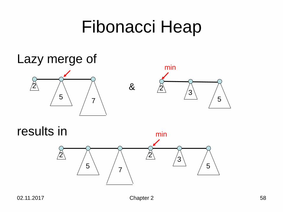
Fibonacci Heap
Lazy merge of
results in
25
2 357
&
25
2 357
min
min
02.11.2017 Chapter 2 59
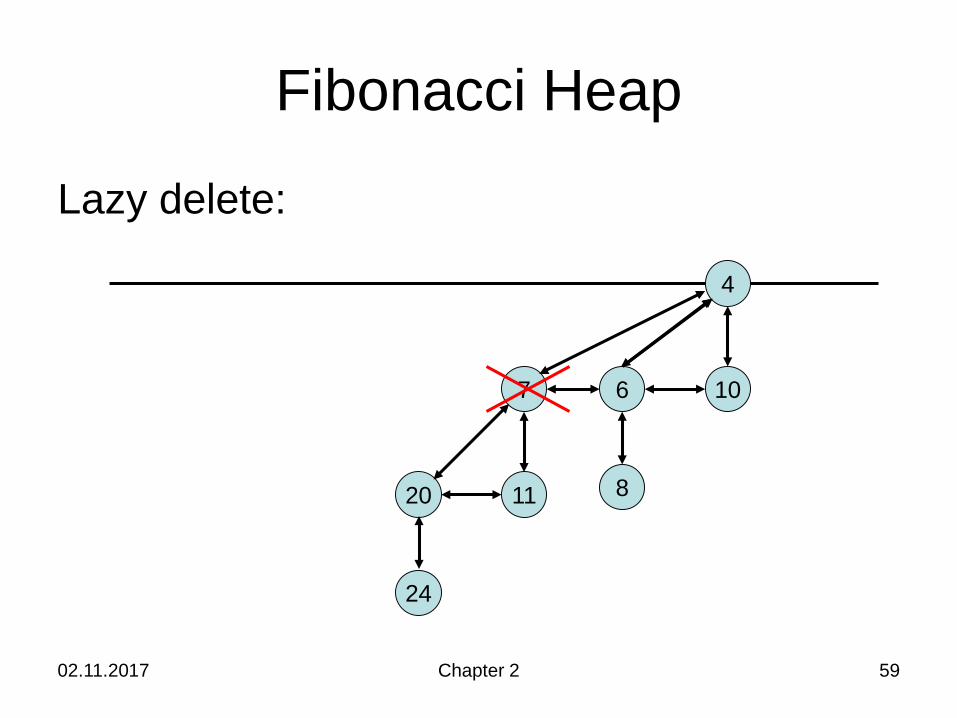
Fibonacci Heap
Lazy delete:
4
106
8
7
1120
24
02.11.2017 Chapter 2 60
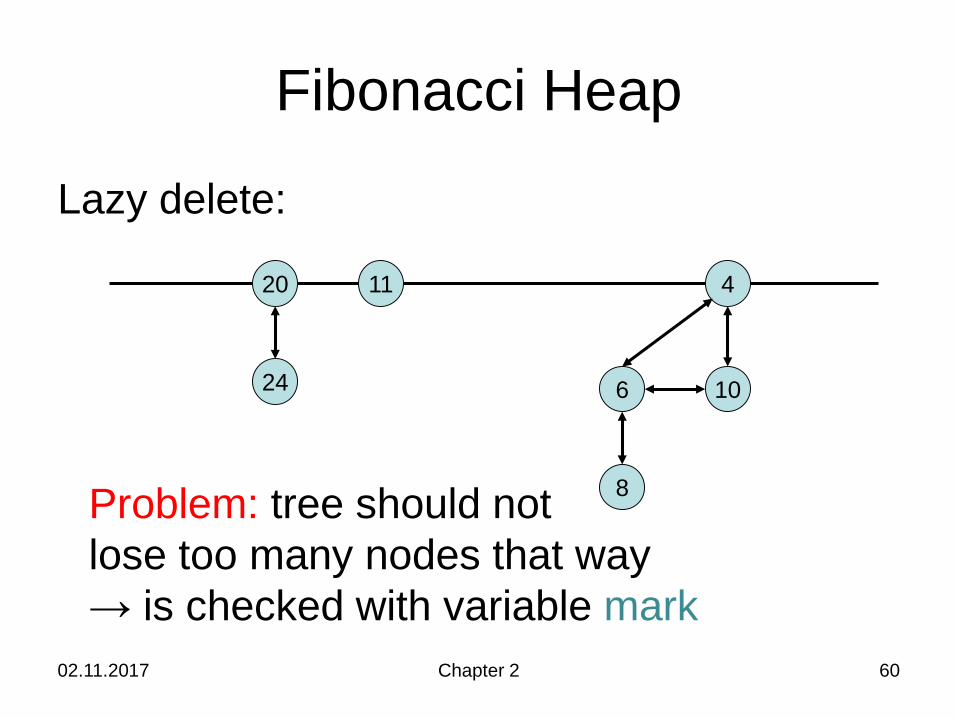
Fibonacci Heap
Lazy delete:
4
106
8Problem: tree should not lose too many nodes that way → is checked with variable mark
1120
24
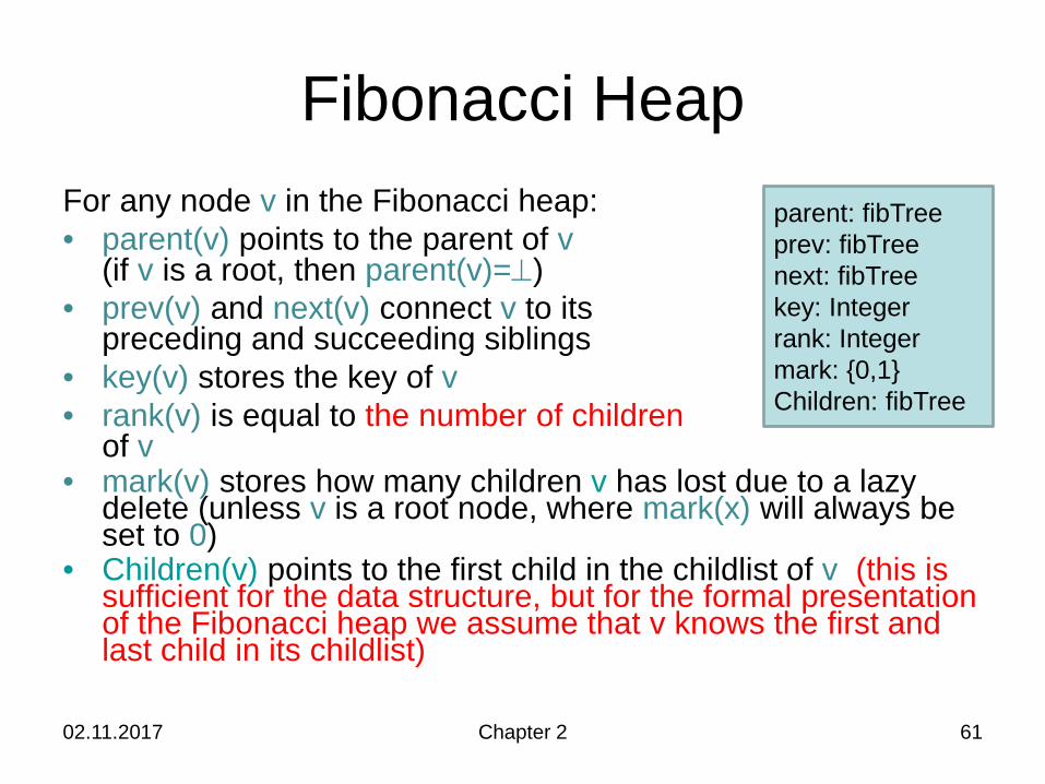
Fibonacci HeapFor any node v in the Fibonacci heap:• parent(v) points to the parent of v
(if v is a root, then parent(v)=⊥)• prev(v) and next(v) connect v to its
preceding and succeeding siblings• key(v) stores the key of v• rank(v) is equal to the number of children
of v• mark(v) stores how many children v has lost due to a lazy
delete (unless v is a root node, where mark(x) will always be set to 0)
• Children(v) points to the first child in the childlist of v (this is sufficient for the data structure, but for the formal presentation of the Fibonacci heap we assume that v knows the first and last child in its childlist)
02.11.2017 Chapter 2 61
parent: fibTreeprev: fibTreenext: fibTreekey: Integerrank: Integermark: {0,1}Children: fibTree
02.11.2017 Chapter 2 62
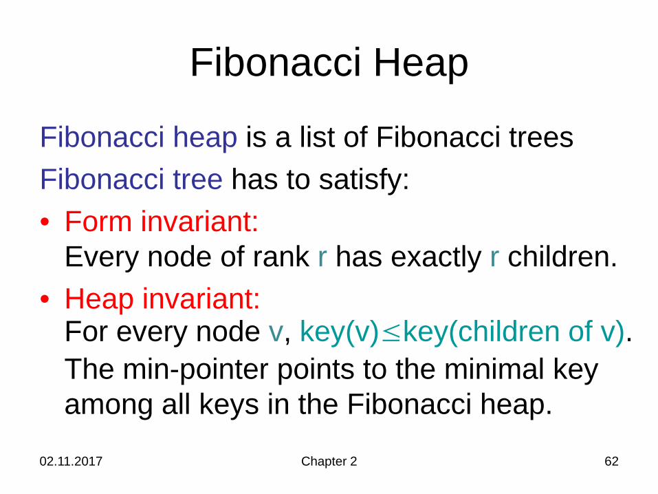
Fibonacci Heap
Fibonacci heap is a list of Fibonacci treesFibonacci tree has to satisfy:• Form invariant:
Every node of rank r has exactly r children.• Heap invariant:
For every node v, key(v)≤key(children of v).The min-pointer points to the minimal keyamong all keys in the Fibonacci heap.
02.11.2017 Chapter 2 63
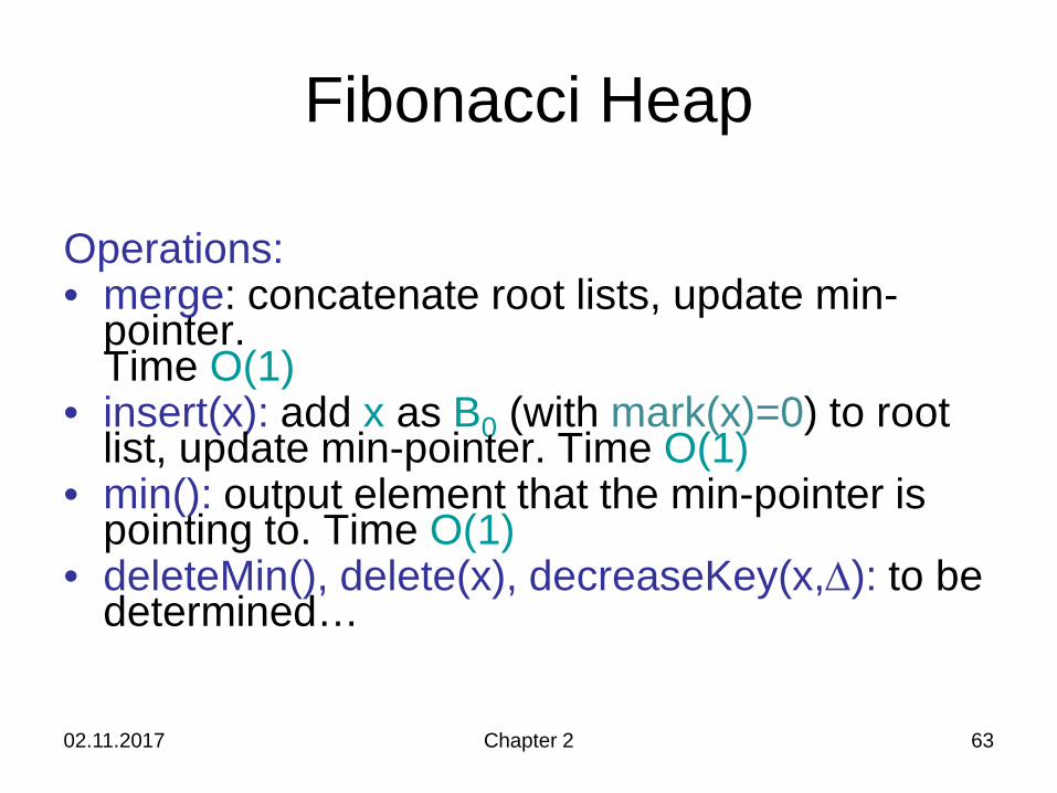
Fibonacci Heap
Operations:• merge: concatenate root lists, update min-
pointer. Time O(1)
• insert(x): add x as B0 (with mark(x)=0) to root list, update min-pointer. Time O(1)
• min(): output element that the min-pointer is pointing to. Time O(1)
• deleteMin(), delete(x), decreaseKey(x,∆): to be determined…
02.11.2017 Chapter 2 64
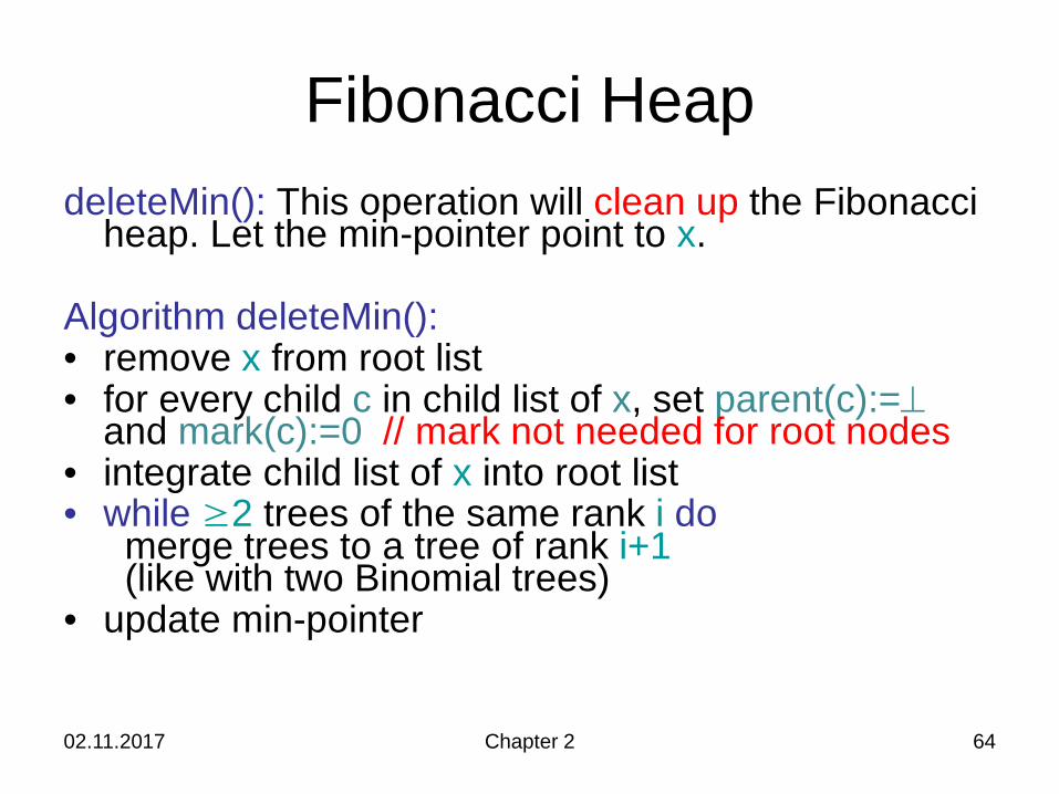
Fibonacci HeapdeleteMin(): This operation will clean up the Fibonacci
heap. Let the min-pointer point to x.
Algorithm deleteMin():• remove x from root list• for every child c in child list of x, set parent(c):=⊥
and mark(c):=0 // mark not needed for root nodes• integrate child list of x into root list• while ≥2 trees of the same rank i do
merge trees to a tree of rank i+1(like with two Binomial trees)
• update min-pointer
02.11.2017 Chapter 2 65
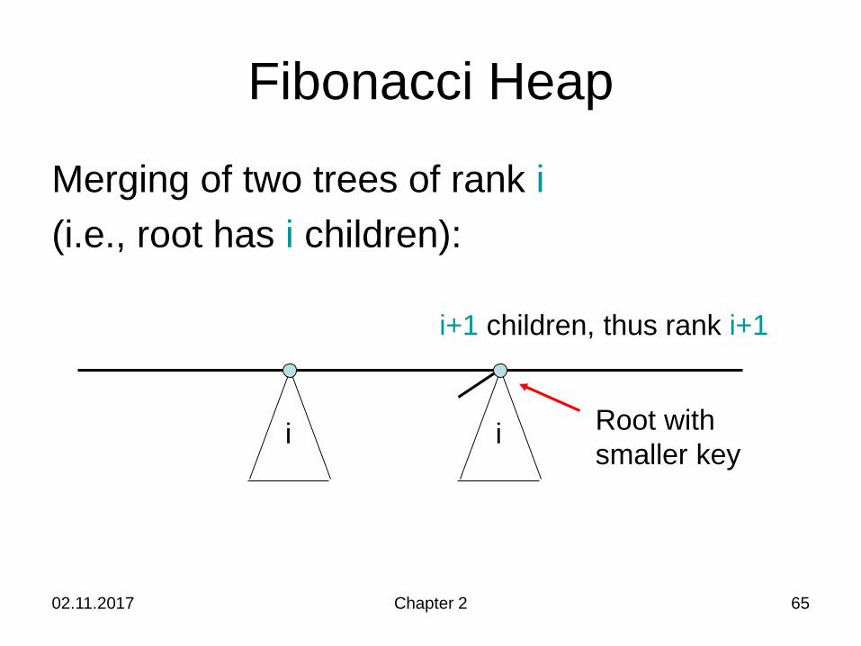
Fibonacci Heap
Merging of two trees of rank i(i.e., root has i children):
i i Root withsmaller key
i+1 children, thus rank i+1
02.11.2017 Chapter 2 66
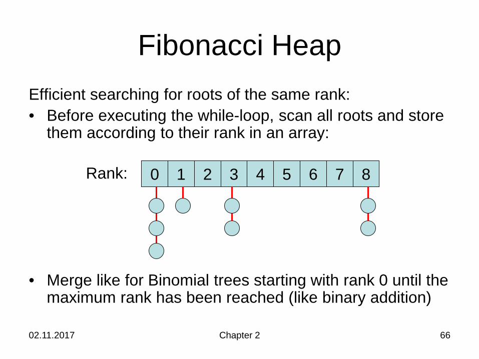
Fibonacci HeapEfficient searching for roots of the same rank:• Before executing the while-loop, scan all roots and store
them according to their rank in an array:
• Merge like for Binomial trees starting with rank 0 until the maximum rank has been reached (like binary addition)
0 21 3 4 5 6 7 8Rank:
02.11.2017 Chapter 2 67
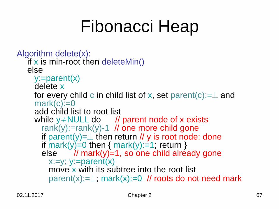
Fibonacci HeapAlgorithm delete(x):
if x is min-root then deleteMin()else
y:=parent(x)delete xfor every child c in child list of x, set parent(c):=⊥ and mark(c):=0add child list to root list while y≠NULL do // parent node of x exists
rank(y):=rank(y)-1 // one more child goneif parent(y)=⊥ then return // y is root node: doneif mark(y)=0 then { mark(y):=1; return }else // mark(y)=1, so one child already gone
x:=y; y:=parent(x)move x with its subtree into the root listparent(x):=⊥; mark(x):=0 // roots do not need mark
02.11.2017 Chapter 2 68
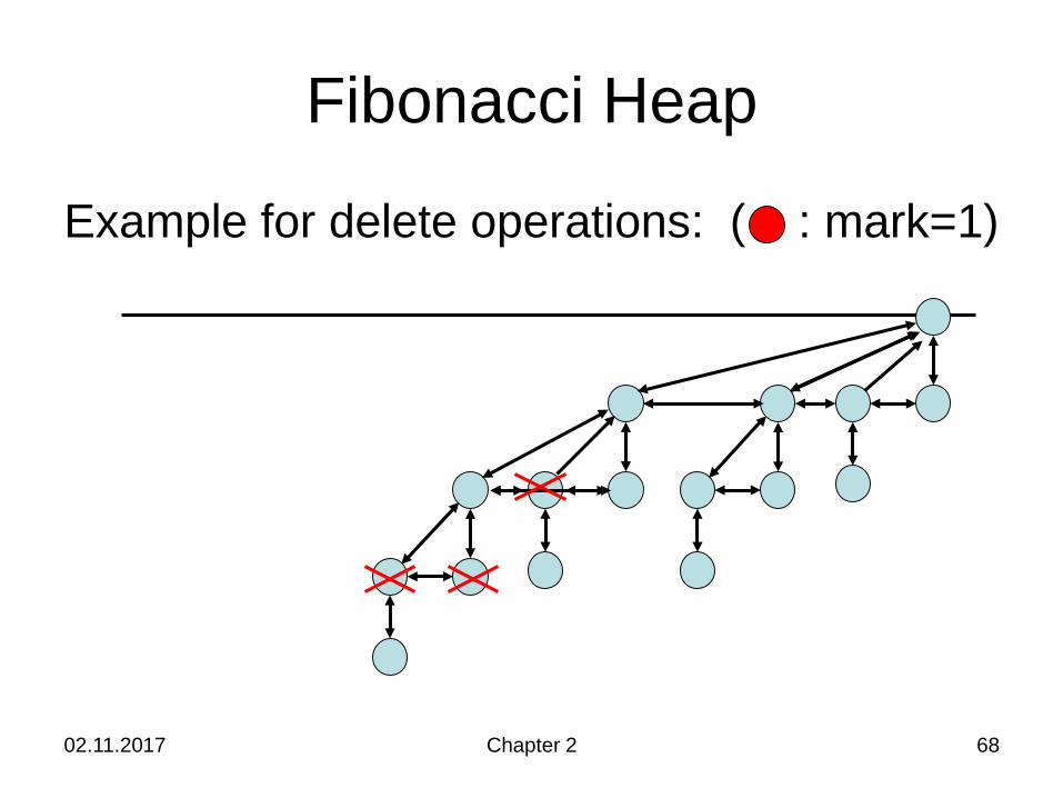
Fibonacci Heap
Example for delete operations: ( : mark=1)
02.11.2017 Chapter 2 69
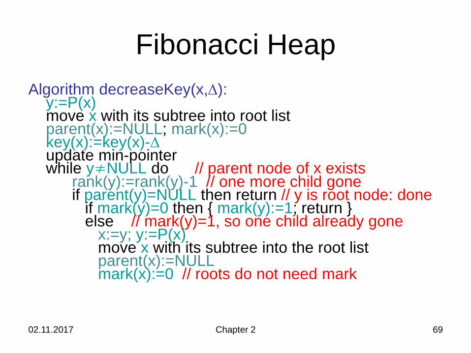
Fibonacci HeapAlgorithm decreaseKey(x,∆):
y:=P(x)move x with its subtree into root listparent(x):=NULL; mark(x):=0key(x):=key(x)-∆update min-pointerwhile y≠NULL do // parent node of x exists
rank(y):=rank(y)-1 // one more child goneif parent(y)=NULL then return // y is root node: done
if mark(y)=0 then { mark(y):=1; return }else // mark(y)=1, so one child already gone
x:=y; y:=P(x)move x with its subtree into the root listparent(x):=NULLmark(x):=0 // roots do not need mark
02.11.2017 Chapter 2 70
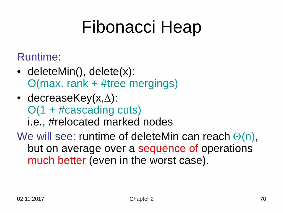
Fibonacci HeapRuntime:• deleteMin(), delete(x):
O(max. rank + #tree mergings)• decreaseKey(x,∆):
O(1 + #cascading cuts)i.e., #relocated marked nodes
We will see: runtime of deleteMin can reach Θ(n), but on average over a sequence of operations much better (even in the worst case).
02.11.2017 Chapter 2 71
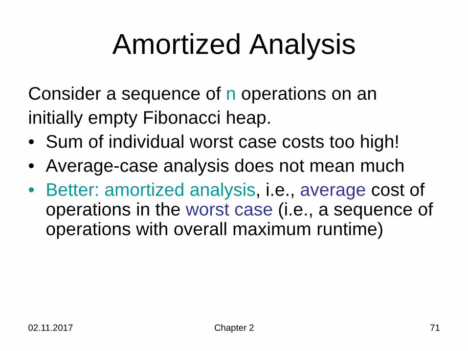
Amortized AnalysisConsider a sequence of n operations on an initially empty Fibonacci heap.• Sum of individual worst case costs too high!• Average-case analysis does not mean much• Better: amortized analysis, i.e., average cost of
operations in the worst case (i.e., a sequence of operations with overall maximum runtime)
02.11.2017 Chapter 2 72
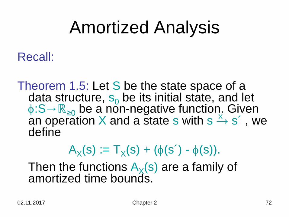
Amortized AnalysisRecall:
Theorem 1.5: Let S be the state space of a data structure, s0 be its initial state, and letφ:S→ℝ≥0 be a non-negative function. Given an operation X and a state s with s → s´ , we define
AX(s) := TX(s) + (φ(s´) - φ(s)).Then the functions AX(s) are a family of amortized time bounds.
X
02.11.2017 Chapter 2 73
Amortized Analysis
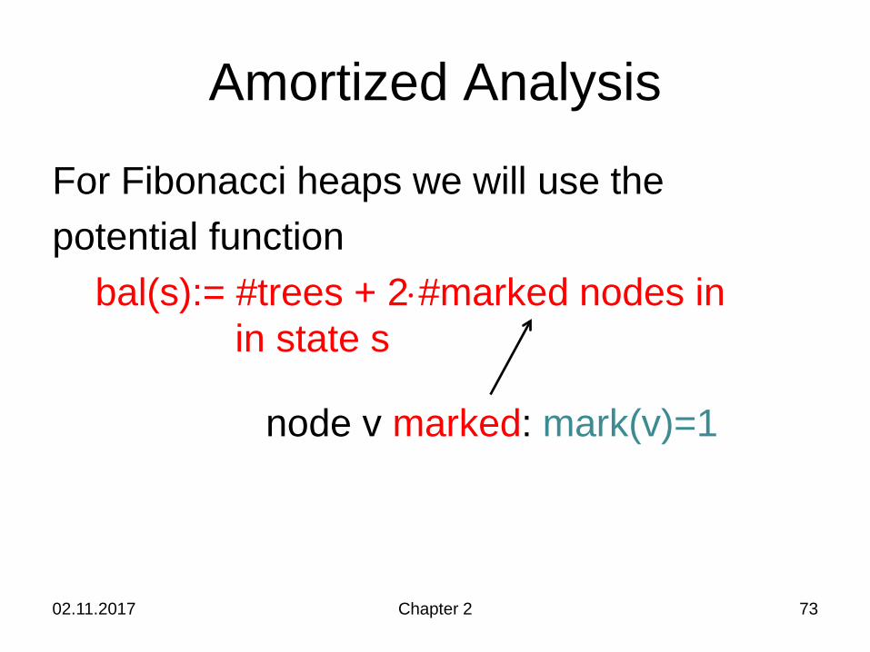
For Fibonacci heaps we will use the potential function
bal(s):= #trees + 2⋅#marked nodes inin state s
node v marked: mark(v)=1
02.11.2017 Chapter 2 74
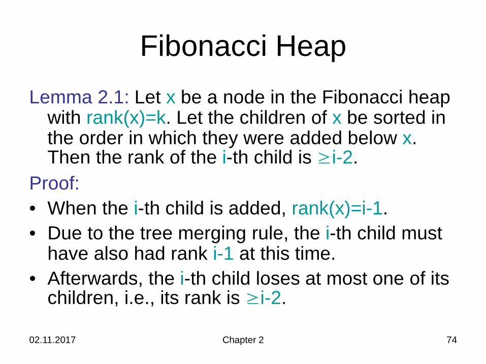
Fibonacci HeapLemma 2.1: Let x be a node in the Fibonacci heap
with rank(x)=k. Let the children of x be sorted in the order in which they were added below x. Then the rank of the i-th child is ≥i-2.
Proof:• When the i-th child is added, rank(x)=i-1.• Due to the tree merging rule, the i-th child must
have also had rank i-1 at this time.• Afterwards, the i-th child loses at most one of its
children, i.e., its rank is ≥i-2.
02.11.2017 Chapter 2 75
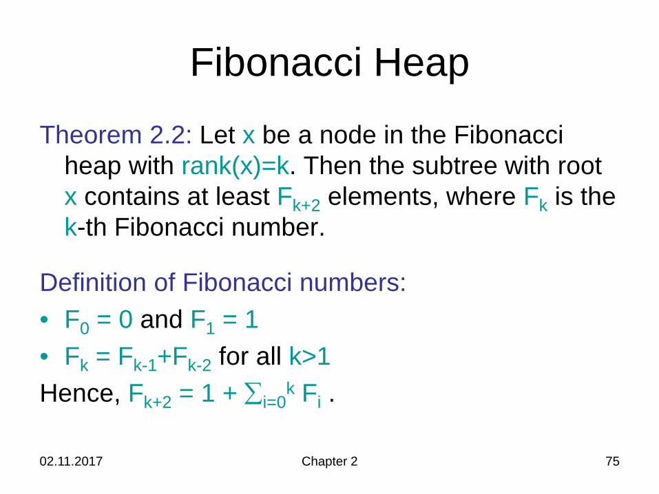
Fibonacci HeapTheorem 2.2: Let x be a node in the Fibonacci
heap with rank(x)=k. Then the subtree with root x contains at least Fk+2 elements, where Fk is the k-th Fibonacci number.
Definition of Fibonacci numbers:• F0 = 0 and F1 = 1• Fk = Fk-1+Fk-2 for all k>1Hence, Fk+2 = 1 + ∑i=0
k Fi .
02.11.2017 Chapter 2 76
Fibonacci Heap
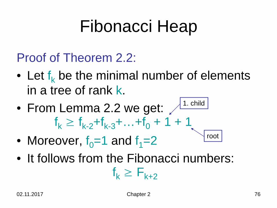
Proof of Theorem 2.2:• Let fk be the minimal number of elements
in a tree of rank k.• From Lemma 2.2 we get:
fk ≥ fk-2+fk-3+…+f0 + 1 + 1• Moreover, f0=1 and f1=2• It follows from the Fibonacci numbers:
fk ≥ Fk+2
1. child
root
02.11.2017 Chapter 2 77
Fibonacci Heap
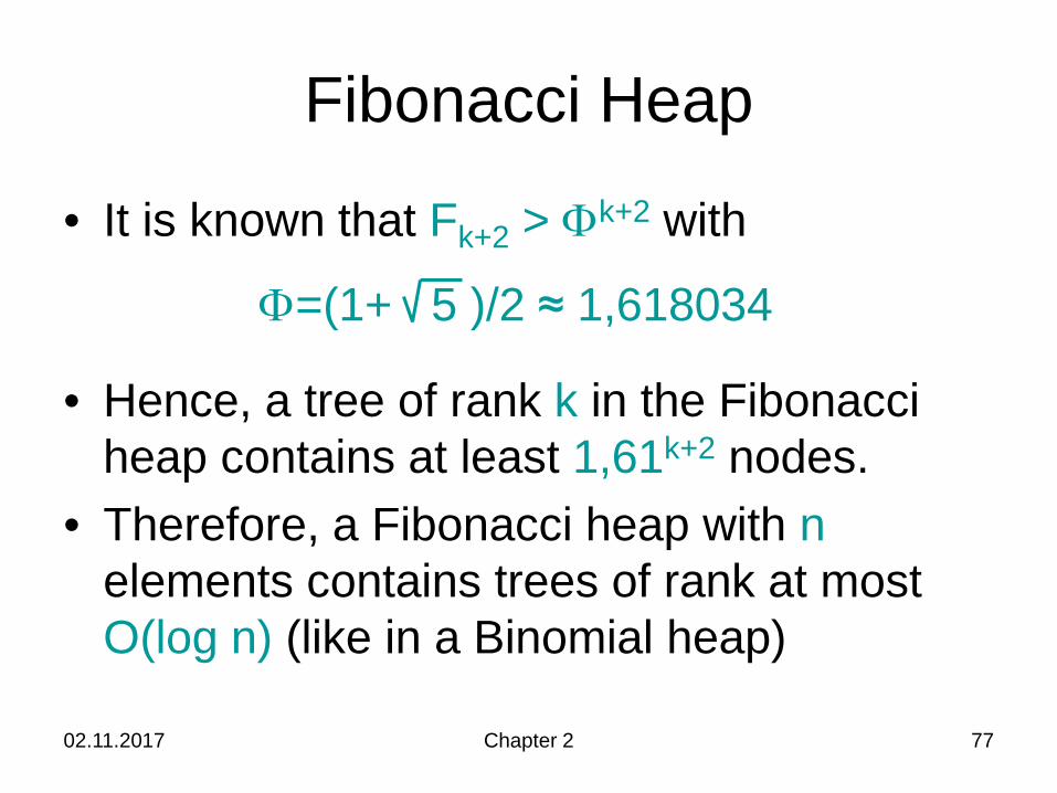
• It is known that Fk+2 > Φk+2 with
Φ=(1+ 5 )/2 ≈ 1,618034
• Hence, a tree of rank k in the Fibonacci heap contains at least 1,61k+2 nodes.
• Therefore, a Fibonacci heap with nelements contains trees of rank at most O(log n) (like in a Binomial heap)
02.11.2017 Chapter 2 78
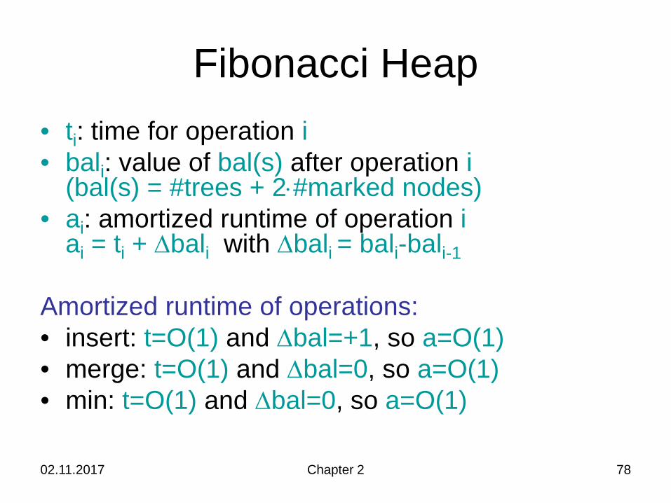
Fibonacci Heap• ti: time for operation i• bali: value of bal(s) after operation i
(bal(s) = #trees + 2⋅#marked nodes)• ai: amortized runtime of operation i
ai = ti + ∆bali with ∆bali = bali-bali-1
Amortized runtime of operations:• insert: t=O(1) and ∆bal=+1, so a=O(1)• merge: t=O(1) and ∆bal=0, so a=O(1)• min: t=O(1) and ∆bal=0, so a=O(1)
02.11.2017 Chapter 2 79
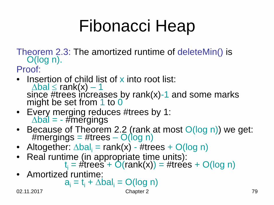
Fibonacci HeapTheorem 2.3: The amortized runtime of deleteMin() is
O(log n).Proof:• Insertion of child list of x into root list:
∆bal ≤ rank(x) – 1 since #trees increases by rank(x)-1 and some marks might be set from 1 to 0
• Every merging reduces #trees by 1:∆bal = - #mergings
• Because of Theorem 2.2 (rank at most O(log n)) we get:#mergings = #trees – O(log n)
• Altogether: ∆bali = rank(x) - #trees + O(log n)• Real runtime (in appropriate time units):
ti = #trees + O(rank(x)) = #trees + O(log n) • Amortized runtime:
ai = ti + ∆bali = O(log n)
02.11.2017 Chapter 2 80
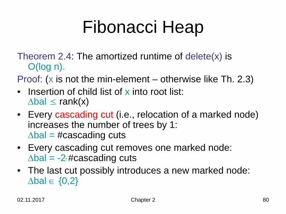
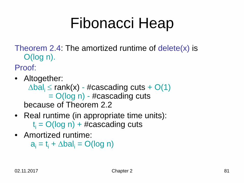
Fibonacci HeapTheorem 2.4: The amortized runtime of delete(x) is
O(log n).Proof: (x is not the min-element – otherwise like Th. 2.3)• Insertion of child list of x into root list:
∆bal ≤ rank(x)• Every cascading cut (i.e., relocation of a marked node)
increases the number of trees by 1:∆bal = #cascading cuts
• Every cascading cut removes one marked node: ∆bal = -2⋅#cascading cuts
• The last cut possibly introduces a new marked node:∆bal ∈ {0,2}
02.11.2017 Chapter 2 81
Fibonacci HeapTheorem 2.4: The amortized runtime of delete(x) is
O(log n).Proof:• Altogether:
∆bali ≤ rank(x) - #cascading cuts + O(1)= O(log n) - #cascading cuts
because of Theorem 2.2• Real runtime (in appropriate time units):
ti = O(log n) + #cascading cuts• Amortized runtime:
ai = ti + ∆bali = O(log n)
02.11.2017 Chapter 2 82
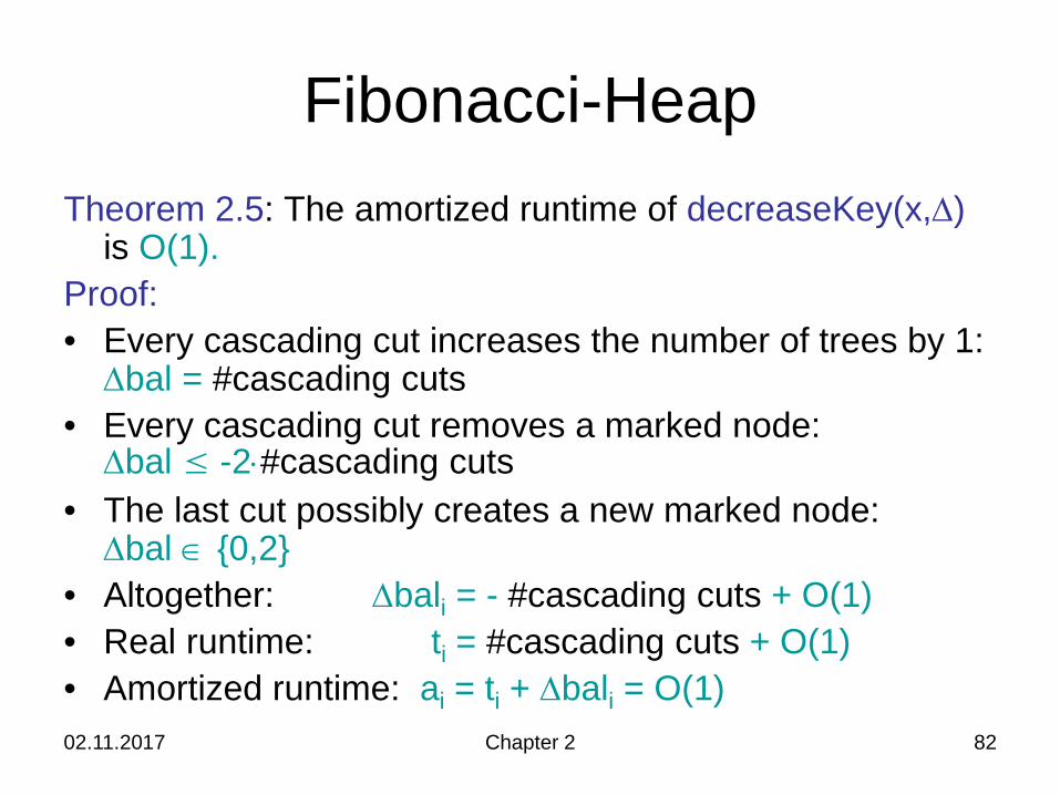
Fibonacci-HeapTheorem 2.5: The amortized runtime of decreaseKey(x,∆)
is O(1).Proof:• Every cascading cut increases the number of trees by 1:
∆bal = #cascading cuts• Every cascading cut removes a marked node:
∆bal ≤ -2⋅#cascading cuts• The last cut possibly creates a new marked node:
∆bal ∈ {0,2}• Altogether: ∆bali = - #cascading cuts + O(1)• Real runtime: ti = #cascading cuts + O(1)• Amortized runtime: ai = ti + ∆bali = O(1)
02.11.2017 Chapter 2 83
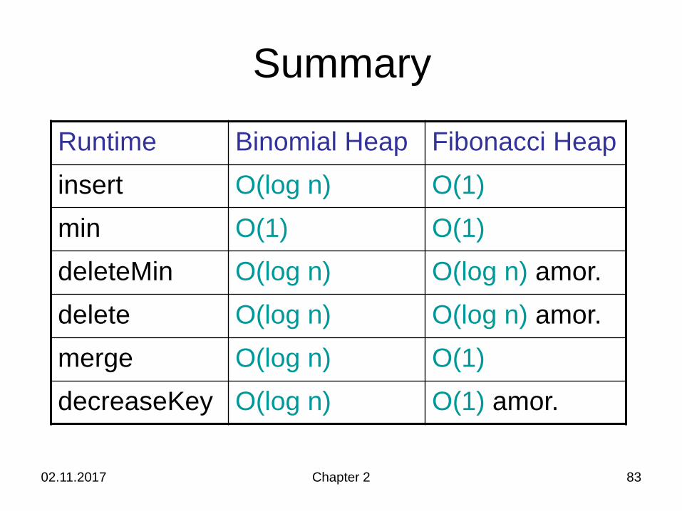
Summary
Runtime Binomial Heap Fibonacci Heapinsert O(log n) O(1)min O(1) O(1)deleteMin O(log n) O(log n) amor.delete O(log n) O(log n) amor.merge O(log n) O(1)decreaseKey O(log n) O(1) amor.
02.11.2017 Chapter 2 84
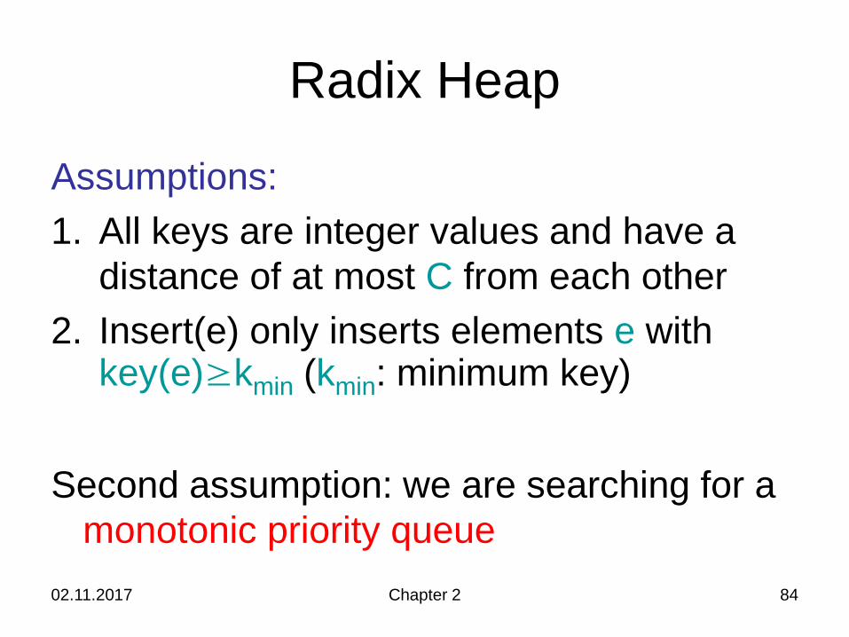
Radix Heap
Assumptions:1. All keys are integer values and have a
distance of at most C from each other2. Insert(e) only inserts elements e with
key(e)≥kmin (kmin: minimum key)
Second assumption: we are searching for a monotonic priority queue
02.11.2017 Chapter 2 85
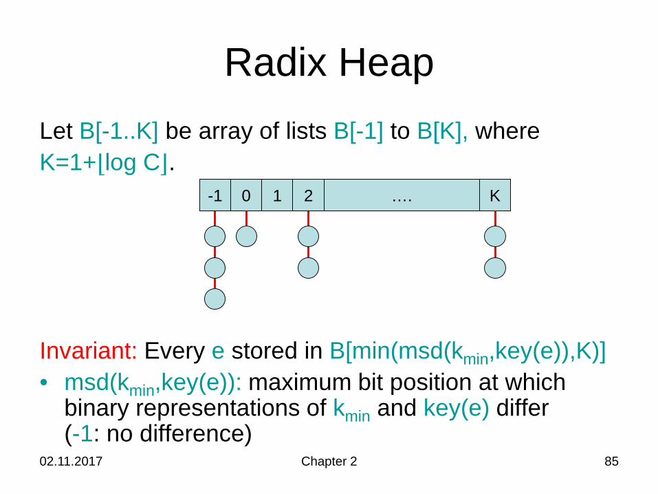
Radix HeapLet B[-1..K] be array of lists B[-1] to B[K], whereK=1+⌊log C⌋.
Invariant: Every e stored in B[min(msd(kmin,key(e)),K)]• msd(kmin,key(e)): maximum bit position at which
binary representations of kmin and key(e) differ (-1: no difference)
-1 0 1 2 …. K
02.11.2017 Chapter 2 86
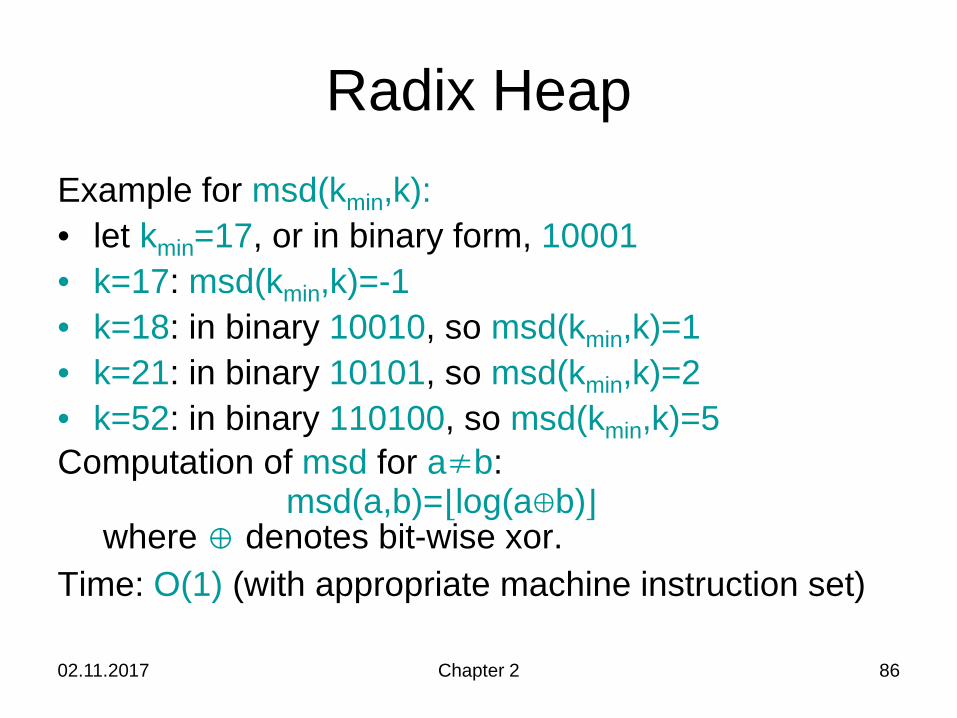
Radix HeapExample for msd(kmin,k):• let kmin=17, or in binary form, 10001• k=17: msd(kmin,k)=-1• k=18: in binary 10010, so msd(kmin,k)=1• k=21: in binary 10101, so msd(kmin,k)=2• k=52: in binary 110100, so msd(kmin,k)=5Computation of msd for a≠b:
msd(a,b)=⌊log(a⊕b)⌋where ⊕ denotes bit-wise xor.
Time: O(1) (with appropriate machine instruction set)
02.11.2017 Chapter 2 87
Radix Heap
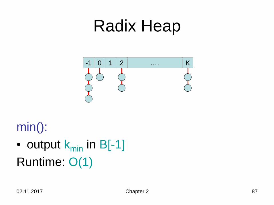
min():• output kmin in B[-1]Runtime: O(1)
-1 0 1 2 …. K
02.11.2017 Chapter 2 88
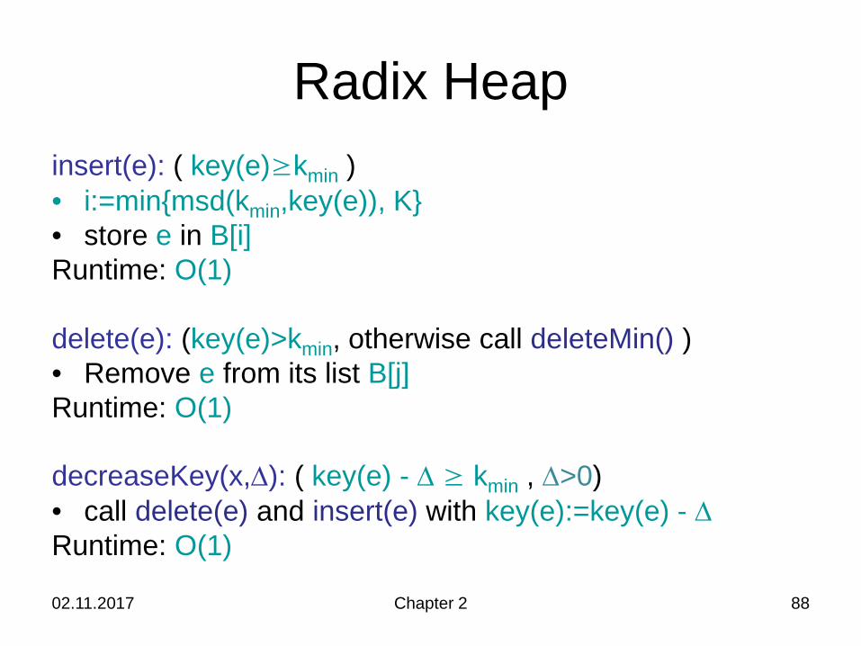
Radix Heapinsert(e): ( key(e)≥kmin )• i:=min{msd(kmin,key(e)), K}• store e in B[i]Runtime: O(1)
delete(e): (key(e)>kmin, otherwise call deleteMin() )• Remove e from its list B[j]Runtime: O(1)
decreaseKey(x,∆): ( key(e) - ∆ ≥ kmin , ∆>0)• call delete(e) and insert(e) with key(e):=key(e) - ∆Runtime: O(1)
02.11.2017 Chapter 2 89
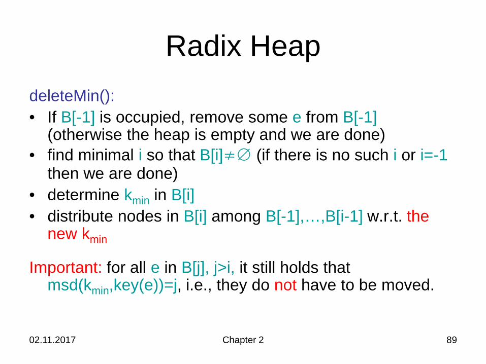
Radix HeapdeleteMin():• If B[-1] is occupied, remove some e from B[-1]
(otherwise the heap is empty and we are done)• find minimal i so that B[i]≠∅ (if there is no such i or i=-1
then we are done)• determine kmin in B[i]• distribute nodes in B[i] among B[-1],…,B[i-1] w.r.t. the
new kmin
Important: for all e in B[j], j>i, it still holds that msd(kmin,key(e))=j, i.e., they do not have to be moved.
02.11.2017 Chapter 2 90
Radix Heap
-1
2
0
5
1
4
2
6
3
9
4
381
5 6 7 8
260
14
11
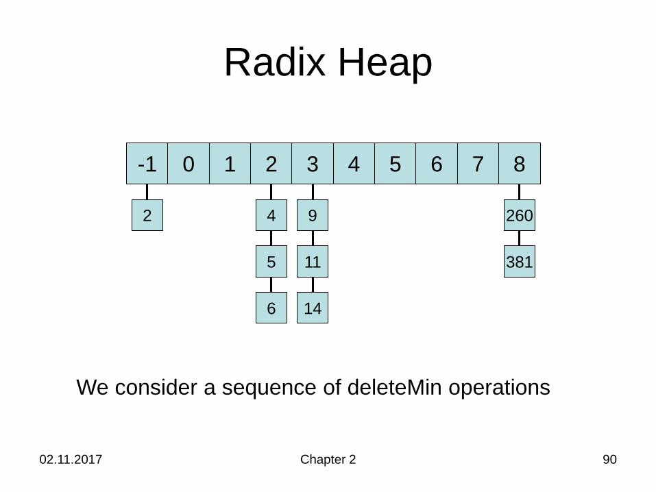
We consider a sequence of deleteMin operations
02.11.2017 Chapter 2 91
Radix Heap
-1 0 1 2 3
9
4
381
5 6 7 8
2601411
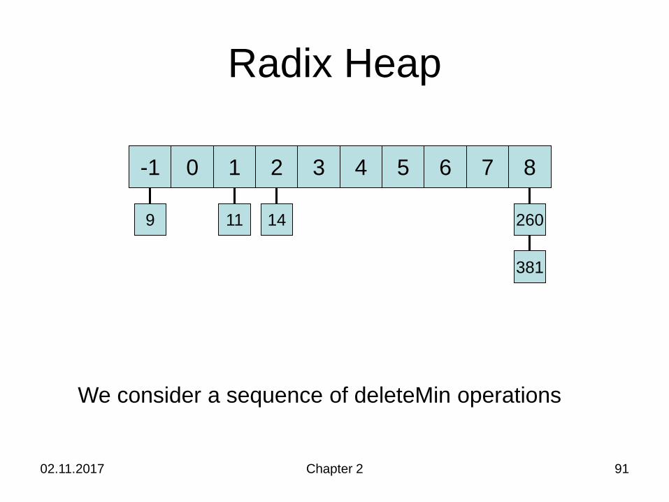
We consider a sequence of deleteMin operations
02.11.2017 Chapter 2 92
Radix Heap
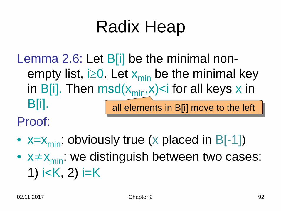
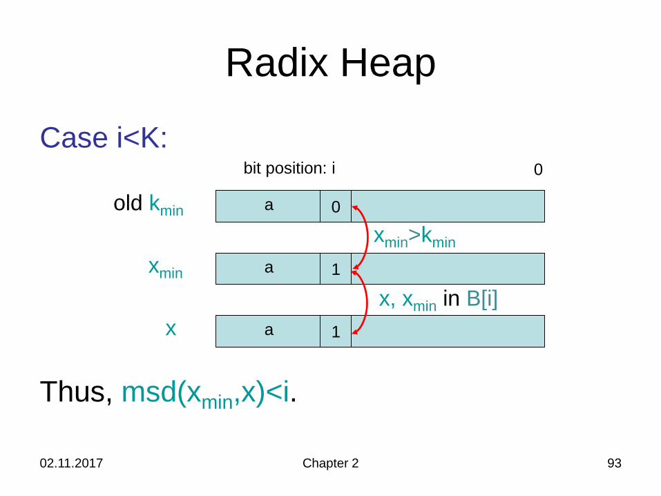
Lemma 2.6: Let B[i] be the minimal non-empty list, i≥0. Let xmin be the minimal key in B[i]. Then msd(xmin,x)<i for all keys x in B[i].
Proof:• x=xmin: obviously true (x placed in B[-1])• x≠xmin: we distinguish between two cases:
1) i<K, 2) i=K
all elements in B[i] move to the left
02.11.2017 Chapter 2 93
Radix Heap
Case i<K:
Thus, msd(xmin,x)<i.
0aold kmin
1axmin
bit position: i
1ax
0
xmin>kmin
x, xmin in B[i]
02.11.2017 Chapter 2 94
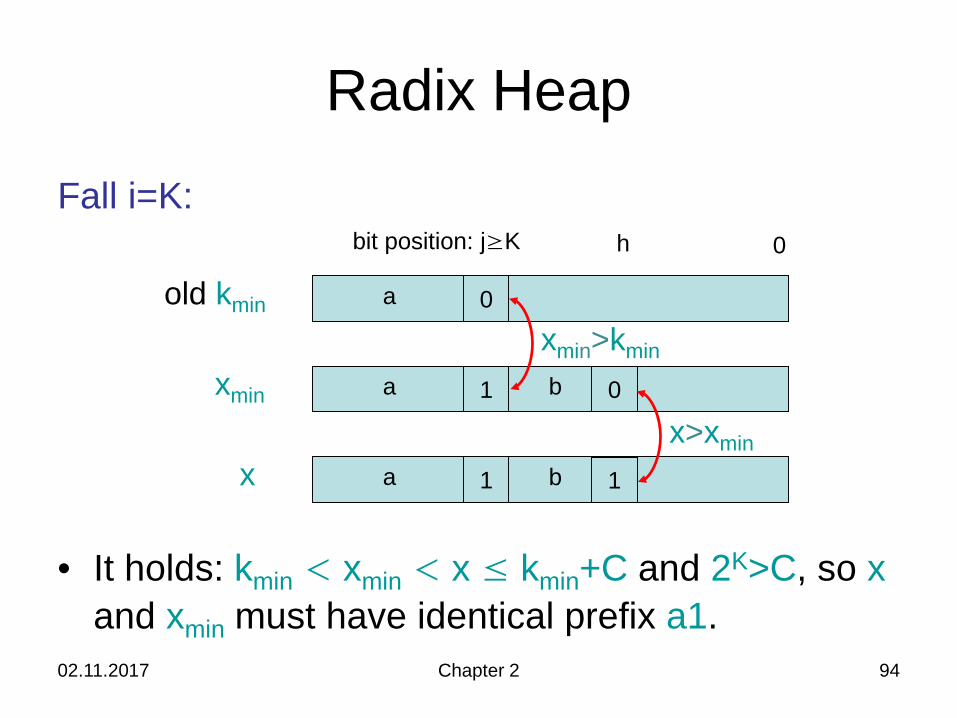
Radix HeapFall i=K:
• It holds: kmin < xmin < x ≤ kmin+C and 2K>C, so x and xmin must have identical prefix a1.
0aold kmin
1axmin
1ax
bit position: j≥K 0h
0
1b
b
xmin>kmin
x>xmin
02.11.2017 Chapter 2 95
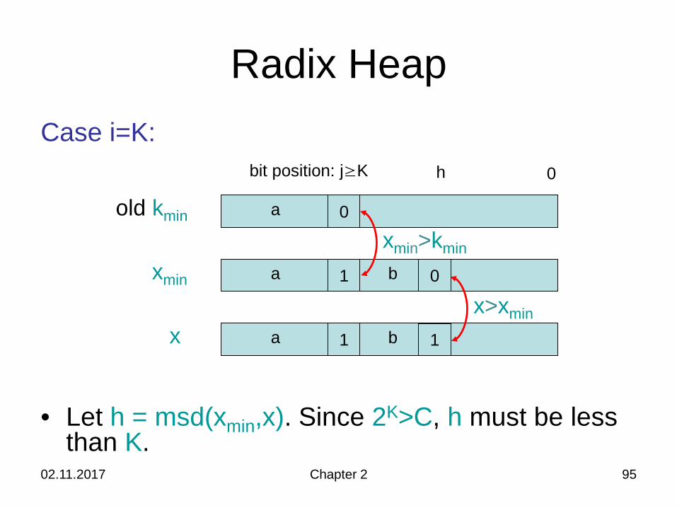
Radix HeapCase i=K:
• Let h = msd(xmin,x). Since 2K>C, h must be lessthan K.
0aold kmin
1axmin
1ax
0h
0
1b
b
bit position: j≥K
xmin>kmin
x>xmin
02.11.2017 Chapter 2 96
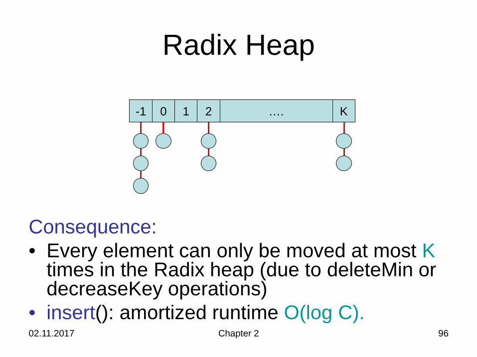
Radix Heap
Consequence:• Every element can only be moved at most K
times in the Radix heap (due to deleteMin ordecreaseKey operations)
• insert(): amortized runtime O(log C).
-1 0 1 2 …. K
02.11.2017 Chapter 2 97
Summary
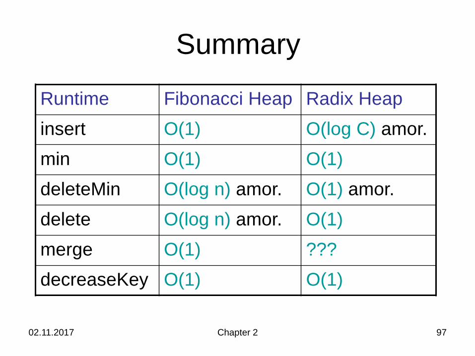
Runtime Fibonacci Heap Radix Heapinsert O(1) O(log C) amor.min O(1) O(1)deleteMin O(log n) amor. O(1) amor.delete O(log n) amor. O(1)merge O(1) ???decreaseKey O(1) O(1)
02.11.2017 Chapter 2 98
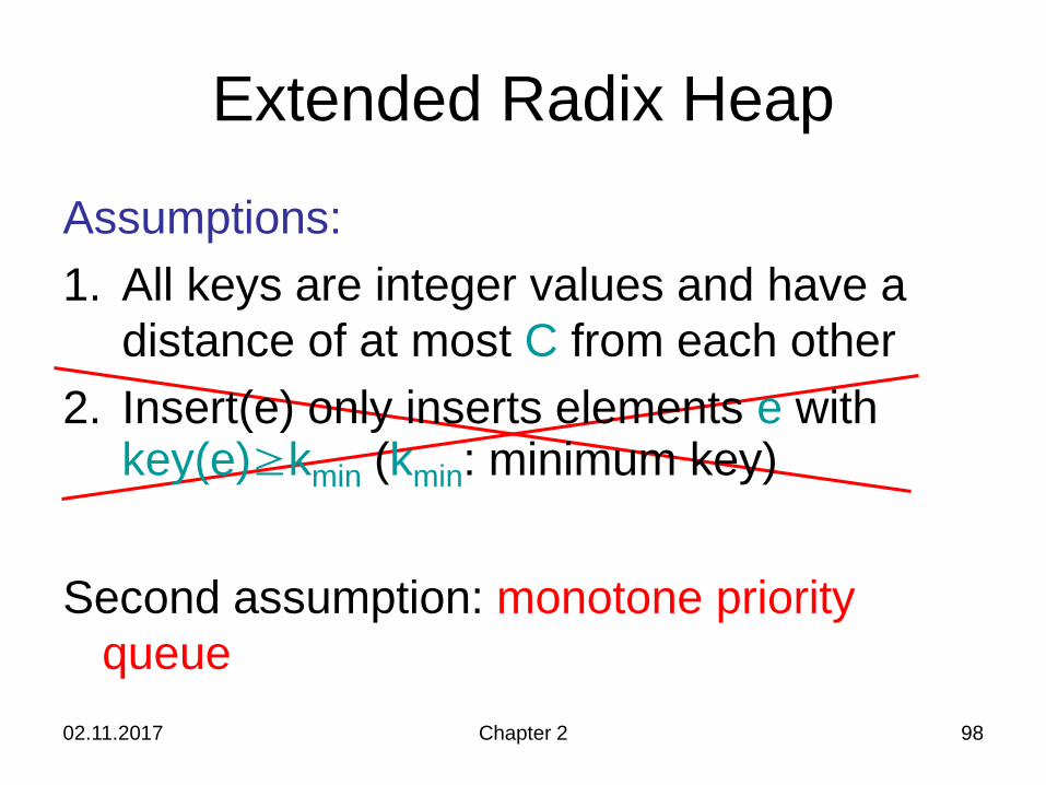
Extended Radix Heap
Assumptions:1. All keys are integer values and have a
distance of at most C from each other2. Insert(e) only inserts elements e with
key(e)≥kmin (kmin: minimum key)
Second assumption: monotone priority queue
02.11.2017 Chapter 2 99
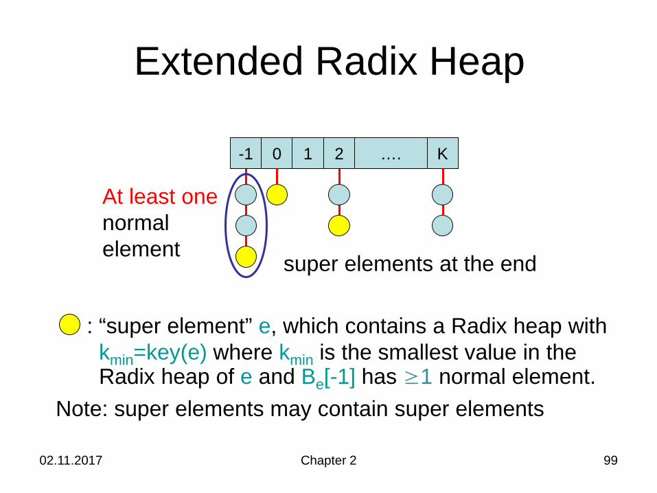
Extended Radix Heap
: “super element” e, which contains a Radix heap with kmin=key(e) where kmin is the smallest value in theRadix heap of e and Be[-1] has ≥1 normal element.
Note: super elements may contain super elements
-1 0 1 2 …. K
At least one normalelement super elements at the end
02.11.2017 Chapter 2 100
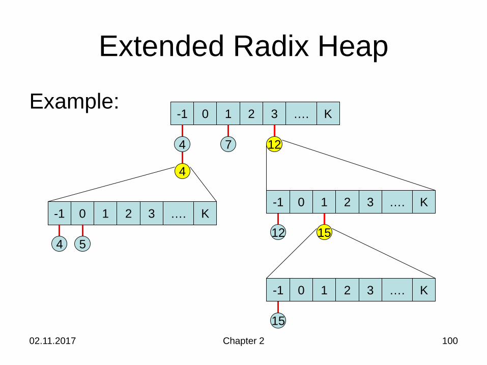
Extended Radix Heap
Example:-1 0 1 2 …. K
4
4 7 12
3
-1 0 1 2 …. K3-1 0 1 2 …. K3
12 154 5
-1 0 1 2 …. K3
15
02.11.2017 Chapter 2 101
Extended Radix Heap
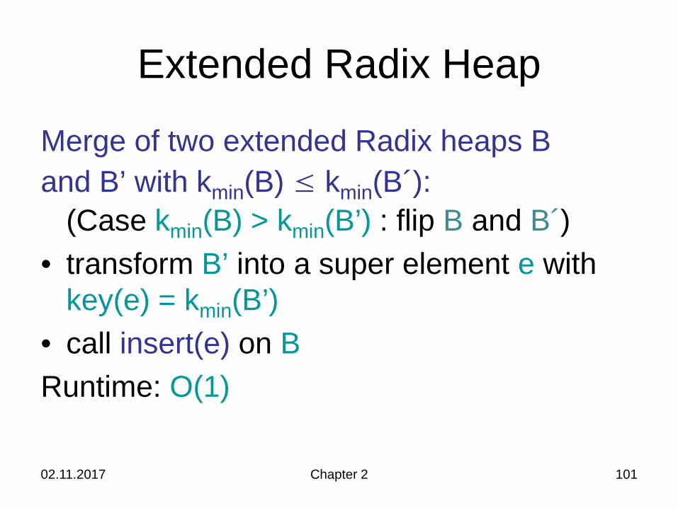
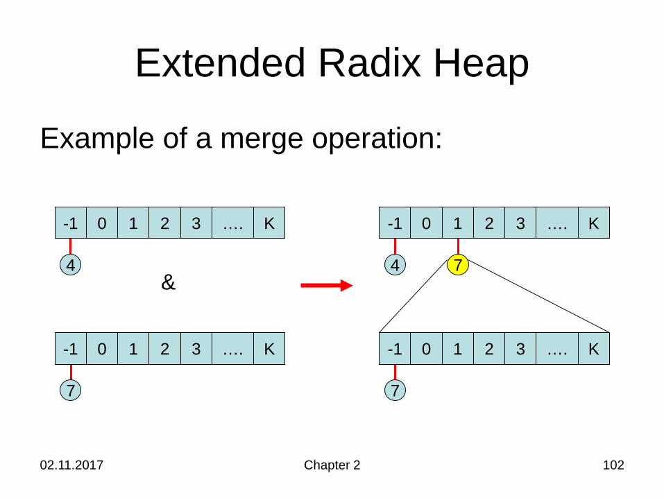
Merge of two extended Radix heaps B and B’ with kmin(B) ≤ kmin(B´):
(Case kmin(B) > kmin(B’) : flip B and B´)• transform B’ into a super element e with
key(e) = kmin(B’)• call insert(e) on BRuntime: O(1)
02.11.2017 Chapter 2 102
Extended Radix Heap
Example of a merge operation:
-1 0 1 2 …. K
4
7
3
-1 0 1 2 …. K3
&
-1 0 1 2 …. K
4
3
7
7
-1 0 1 2 …. K3
02.11.2017 Chapter 2 103
Extended Radix Heapinsert(e): • key(e)≥kmin: as in standard Radix heap• otherwise, merge extended Radix heap
with a new Radix heap just containing eRuntime: O(1)
min(): like in a standard Radix heapRuntime: O(1)
02.11.2017 Chapter 2 104
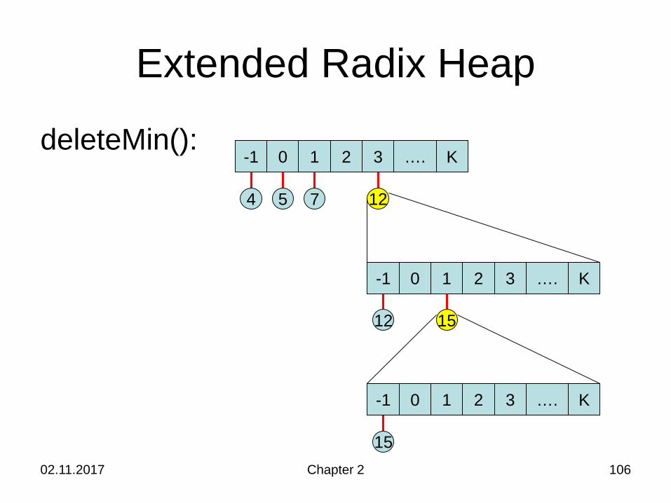
Extended Radix HeapdeleteMin():• Remove normal element e from B[-1]
(B: Radix heap at highest level)• If B[-1] does not contain any elements, then
update B like in a standard Radix heap (i.e., dissolve smallest non-empty bucket B[i])
• If B[-1] does not contain normal elements any more, then take the first super element e’ from B[-1] and merge the lists of e’ with B(then there is again a normal element in B[-1]!)
Runtime: O(log C) + time for updates
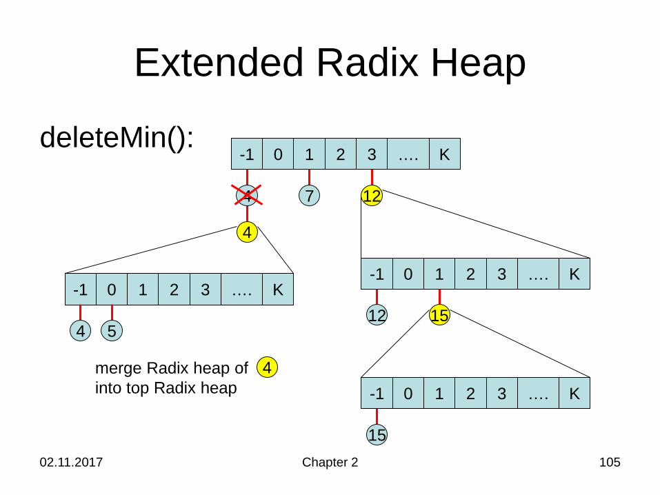
Extended Radix Heap
deleteMin():
02.11.2017 Chapter 2 105
-1 0 1 2 …. K
4
4 7 12
3
-1 0 1 2 …. K3-1 0 1 2 …. K3
12 154 5
-1 0 1 2 …. K3
15
merge Radix heap ofinto top Radix heap
4
Extended Radix Heap
deleteMin():
02.11.2017 Chapter 2 106
-1 0 1 2 …. K
4 7 12
3
-1 0 1 2 …. K3
12 15
5
-1 0 1 2 …. K3
15
02.11.2017 Chapter 2 107
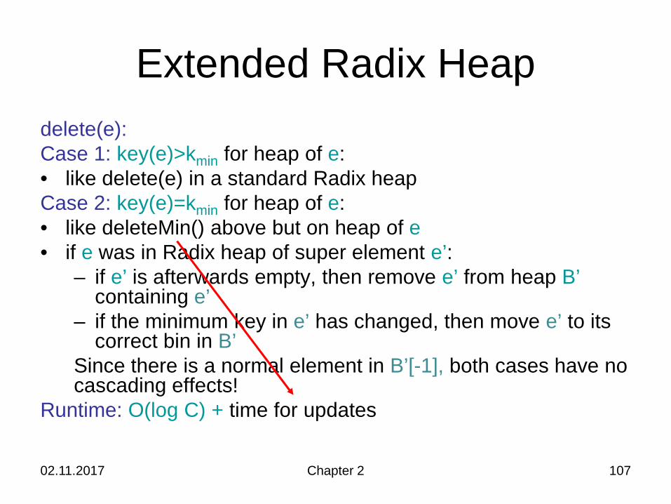
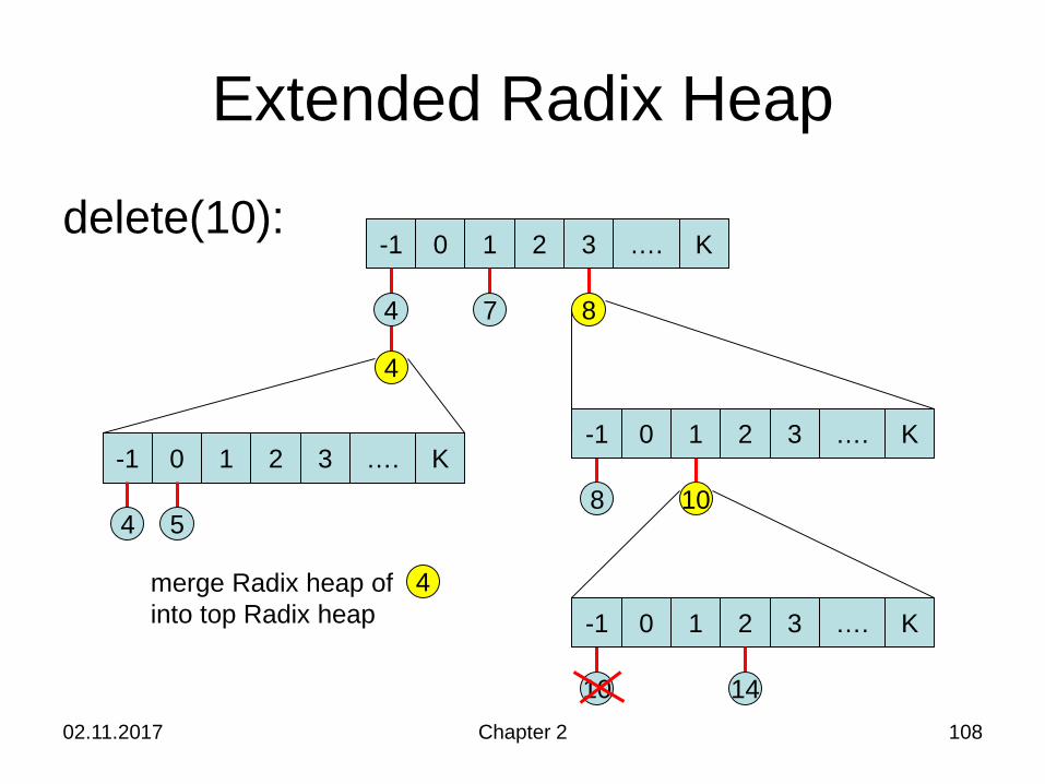
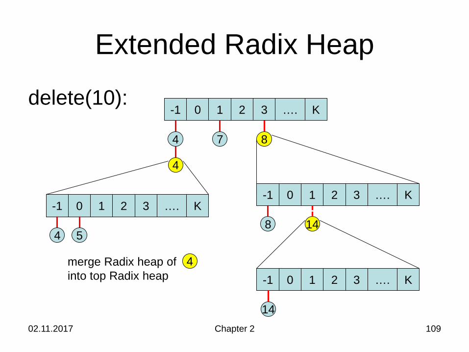
Extended Radix Heapdelete(e):Case 1: key(e)>kmin for heap of e: • like delete(e) in a standard Radix heapCase 2: key(e)=kmin for heap of e: • like deleteMin() above but on heap of e• if e was in Radix heap of super element e’:
– if e’ is afterwards empty, then remove e’ from heap B’containing e’
– if the minimum key in e’ has changed, then move e’ to its correct bin in B’
Since there is a normal element in B’[-1], both cases have no cascading effects!
Runtime: O(log C) + time for updates
Extended Radix Heap
delete(10):
02.11.2017 Chapter 2 108
-1 0 1 2 …. K
4
4 7 8
3
-1 0 1 2 …. K3-1 0 1 2 …. K3
8 104 5
-1 0 1 2 …. K3
10
merge Radix heap ofinto top Radix heap
4
14
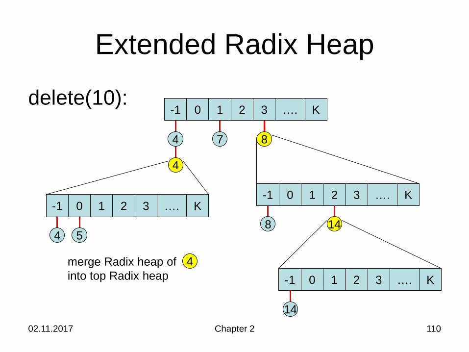
Extended Radix Heap
delete(10):
02.11.2017 Chapter 2 109
-1 0 1 2 …. K
4
4 7 8
3
-1 0 1 2 …. K3-1 0 1 2 …. K3
8 144 5
-1 0 1 2 …. K3merge Radix heap ofinto top Radix heap
4
14
Extended Radix Heap
delete(10):
02.11.2017 Chapter 2 110
-1 0 1 2 …. K
4
4 7 8
3
-1 0 1 2 …. K3-1 0 1 2 …. K3
8 144 5
-1 0 1 2 …. K3merge Radix heap ofinto top Radix heap
4
14
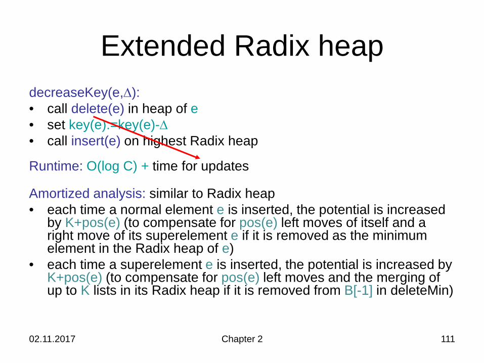
02.11.2017 Chapter 2 111
Extended Radix heapdecreaseKey(e,∆):• call delete(e) in heap of e• set key(e):=key(e)-∆• call insert(e) on highest Radix heap
Runtime: O(log C) + time for updates
Amortized analysis: similar to Radix heap• each time a normal element e is inserted, the potential is increased
by K+pos(e) (to compensate for pos(e) left moves of itself and a right move of its superelement e if it is removed as the minimum element in the Radix heap of e)
• each time a superelement e is inserted, the potential is increased by K+pos(e) (to compensate for pos(e) left moves and the merging of up to K lists in its Radix heap if it is removed from B[-1] in deleteMin)
02.11.2017 Chapter 2 112
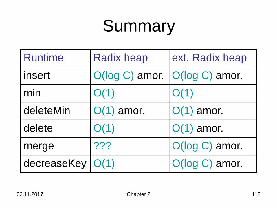
Summary
Runtime Radix heap ext. Radix heapinsert O(log C) amor. O(log C) amor.min O(1) O(1)deleteMin O(1) amor. O(1) amor.delete O(1) O(1) amor.merge ??? O(log C) amor.decreaseKey O(1) O(log C) amor.
Contents
• Binomial heap• Fibonacci heap• Radix heap• Applications
02.11.2017 Chapter 2 113
02.11.2017 Chapter 4 114
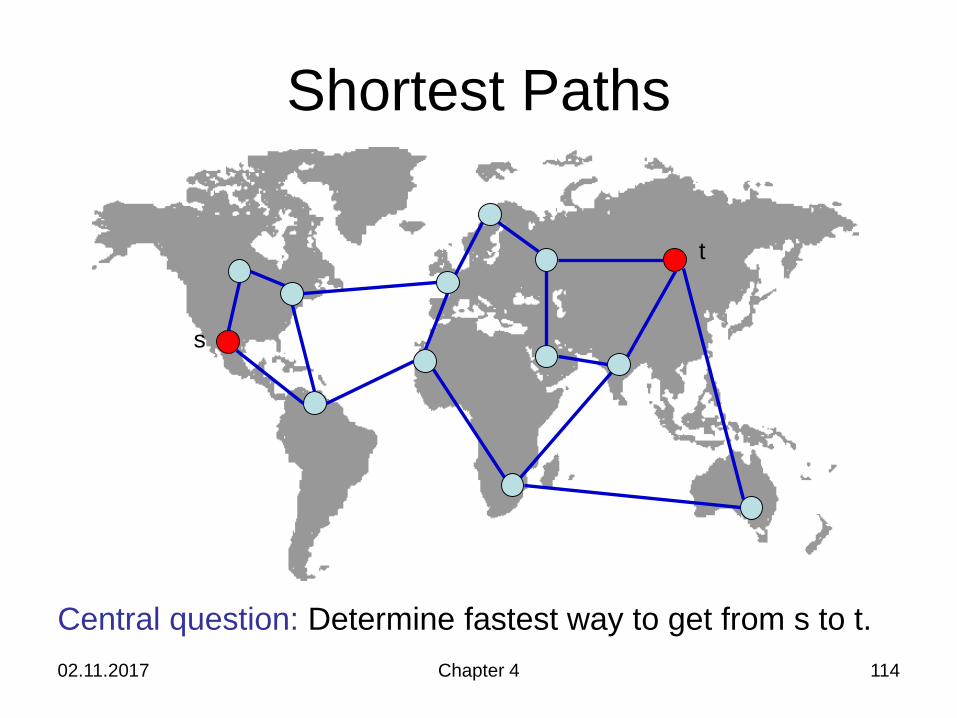
Shortest Paths
Central question: Determine fastest way to get from s to t.
s
t
02.11.2017 Chapter 4 115
Shortest Paths
-∞
+∞ 0
-∞ -∞
-∞
2 -3
-1 -3s
0
-1 -2
-2
5
2-1
0
0
-2
42
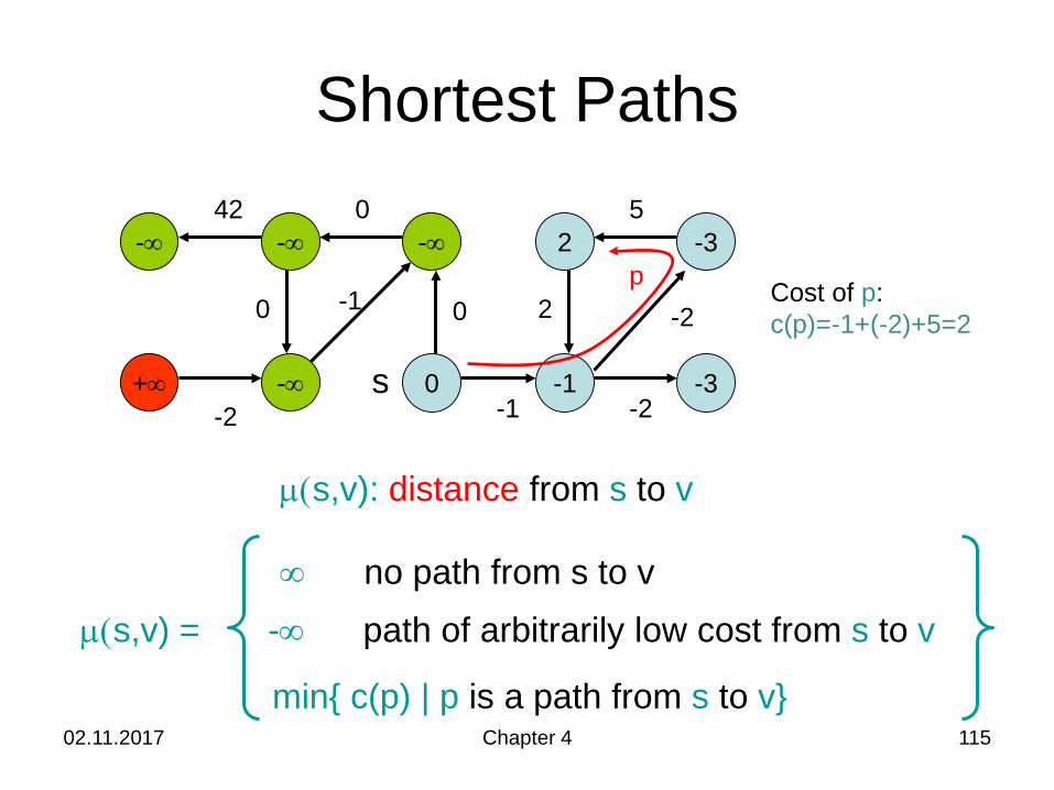
µ(s,v): distance from s to v
µ(s,v) = -∞ path of arbitrarily low cost from s to v∞ no path from s to v
min{ c(p) | p is a path from s to v}
p Cost of p:c(p)=-1+(-2)+5=2
02.11.2017 Chapter 4 116
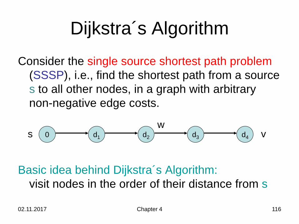
Dijkstra´s AlgorithmConsider the single source shortest path problem
(SSSP), i.e., find the shortest path from a source s to all other nodes, in a graph with arbitrary non-negative edge costs.
Basic idea behind Dijkstra´s Algorithm:visit nodes in the order of their distance from s
0 d1 d2 d3 d4s vw
02.11.2017 Chapter 4 117
Dijkstra´s Algorithm• Initially, set d(s):=0 and d(v):=∞ for all other
nodes. Use a priority queue q in which the priorities represent the current distances d(v)from s. Add s to q.
• Repeat until q is empty:Remove node v with lowest d(v) from q (via deleteMin). For all (v,w)∈E, set d(w) := min{d(w), d(v)+c(v,w)}. If w has not been in q so far, insert w into q. In order to repair q in case of a change of d(w), perform a decreaseKey operation.
02.11.2017 Chapter 4 118
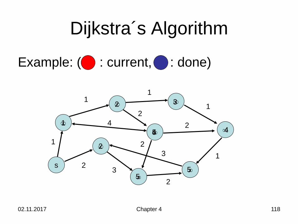
Dijkstra´s Algorithm
Example: ( : current, : done)
s
∞
∞
∞
∞
∞
∞ ∞
∞
1
2
11
1
1
32
24 2
32
1
2
2
5
5
4
3
4
5
02.11.2017 Chapter 4 119
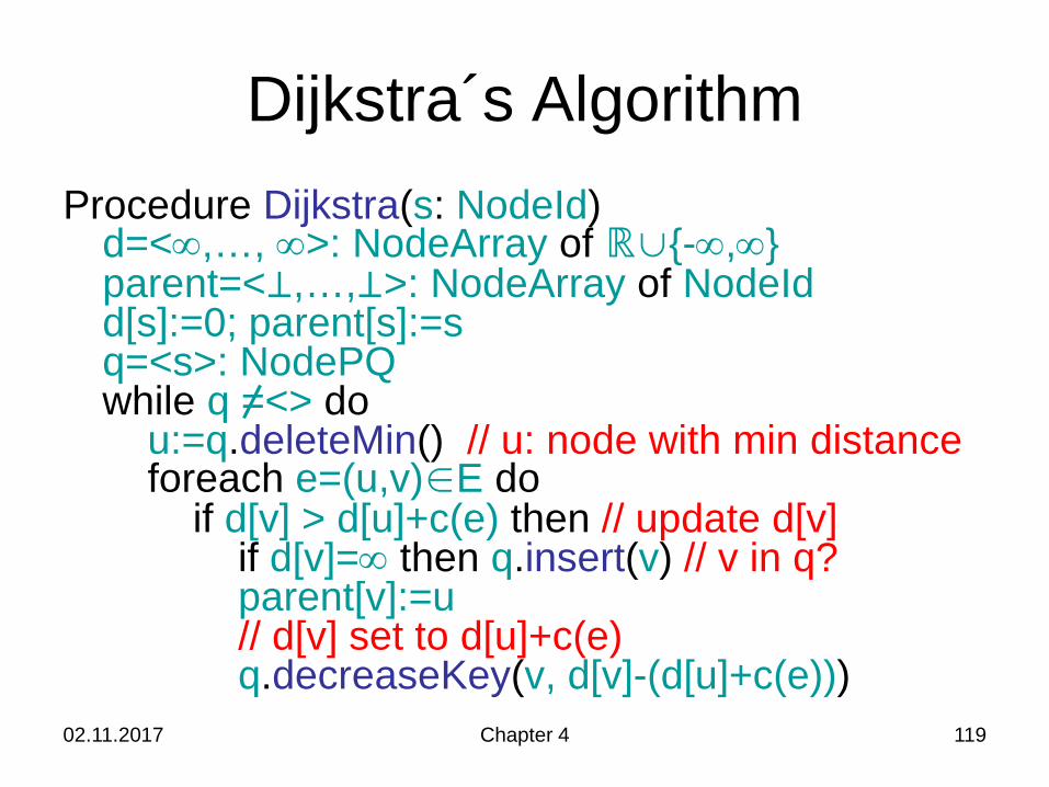
Dijkstra´s AlgorithmProcedure Dijkstra(s: NodeId)
d=<∞,…, ∞>: NodeArray of ℝ∪{-∞,∞}parent=<⊥,…,⊥>: NodeArray of NodeIdd[s]:=0; parent[s]:=sq=<s>: NodePQwhile q =<> do
u:=q.deleteMin() // u: node with min distanceforeach e=(u,v)∈E do
if d[v] > d[u]+c(e) then // update d[v]if d[v]=∞ then q.insert(v) // v in q?parent[v]:=u// d[v] set to d[u]+c(e)q.decreaseKey(v, d[v]-(d[u]+c(e)))
02.11.2017 Chapter 4 120
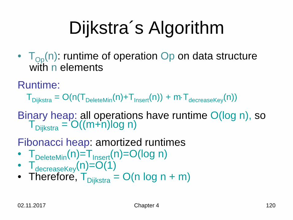
Dijkstra´s Algorithm• TOp(n): runtime of operation Op on data structure
with n elementsRuntime:
TDijkstra = O(n(TDeleteMin(n)+TInsert(n)) + m⋅TdecreaseKey(n))
Binary heap: all operations have runtime O(log n), so TDijkstra = O((m+n)log n)
Fibonacci heap: amortized runtimes• TDeleteMin(n)=TInsert(n)=O(log n)• TdecreaseKey(n)=O(1)• Therefore, TDijkstra = O(n log n + m)
02.11.2017 Chapter 4 121
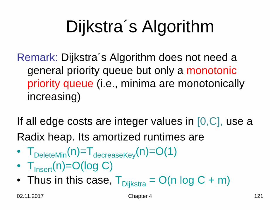
Dijkstra´s AlgorithmRemark: Dijkstra´s Algorithm does not need a
general priority queue but only a monotonic priority queue (i.e., minima are monotonically increasing)
If all edge costs are integer values in [0,C], use a Radix heap. Its amortized runtimes are• TDeleteMin(n)=TdecreaseKey(n)=O(1)• TInsert(n)=O(log C)• Thus in this case, TDijkstra = O(n log C + m)
02.11.2017 Kapitel 11 122
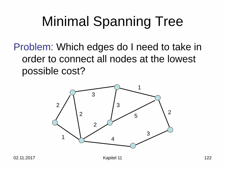
Minimal Spanning Tree
Problem: Which edges do I need to take in order to connect all nodes at the lowest possible cost?
2
1
1
3
3
2
2
43
25
02.11.2017 Kapitel 11 123
Minimal Spanning TreeInput:• Undirected graph G=(V,E)• Edge costs c:E→ℝ+
Output:• Subset T⊆E so that the graph (V,T) is connected
and c(T)=∑e∈T c(e) is minimal
• T always forms a tree (if c is positive).• Tree over all nodes in V with minimum cost:
minimal spanning tree (MST)

02.11.2017 Chapter 4 124
Prim´s AlgorithmProcedure Prim(s: NodeId)
d=<∞,…, ∞>: NodeArray of ℝ∪{-∞,∞}parent=<⊥,…,⊥>: NodeArray of NodeIdd[s]:=0; parent[s]:=sq=<s>: NodePQwhile q =<> do
u:=q.deleteMin() // u: node with min distanceforeach e=(u,v)∈E do
if d[v] > c(e) then // update d[v]if d[v]=∞ then q.insert(v) // v in q?parent[v]:=u// d[v] set to c(e)q.decreaseKey(v, d[v]-c(e))
02.11.2017 Chapter 4 125
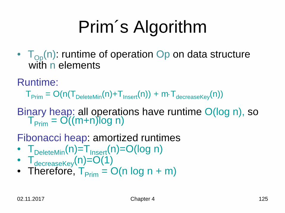
Prim´s Algorithm• TOp(n): runtime of operation Op on data structure
with n elementsRuntime:
TPrim = O(n(TDeleteMin(n)+TInsert(n)) + m⋅TdecreaseKey(n))
Binary heap: all operations have runtime O(log n), so TPrim = O((m+n)log n)
Fibonacci heap: amortized runtimes• TDeleteMin(n)=TInsert(n)=O(log n)• TdecreaseKey(n)=O(1)• Therefore, TPrim = O(n log n + m)

02.11.2017 Chapter 2 126
Next Chapter
Topic: Search structures


![Chapter 9. Heaps [INA240] Data Structures and Practice Youn-Hee Han](https://img.pdfslide.net/doc/110x75/56649f475503460f94c698cf/chapter-9-heaps-ina240-data-structures-and-practice-youn-hee-han-httplinkkutackr.jpg)